Jamming pair of general run-and-tumble particles:
Exact results and universality classes

Abstract

We consider a general system of two run-and-tumble particles interacting by hardcore jamming on the unidimensional torus. RTP are a paradigmatic active matter model, typically modeling the evolution of bacteria. By directly modeling the system at the continuous-space and -time level thanks to piecewise deterministic Markov processes (PDMP), we derive the conservation conditions which sets the invariant distribution and explicitly construct the two universality classes for the steady state, the detailed-jamming and the global-jamming classes. They respectively identify with the preservation or not of a detailed symmetry at the level of the dynamical internal states between probability flows entering and exiting jamming configurations. Thanks to a spectral analysis of the tumble kernel, we give explicit expressions for the invariant measure in the general case. The non-equilibrium features exhibited by the steady state includes positive mass for the jammed configurations and, for the global-jamming class, exponential decay and growth terms, potentially modulated by polynomial terms. Interestingly, we find that the invariant measure follows, away from jamming configurations, a catenary-like constraint, which results from the interplay between probability conservation and the dynamical skewness introduced by the jamming interactions, seen now as a boundary constraint. This work shows the powerful analytical approach PDMP provide for the study of the stationary behaviors of RTP systems and motivates their future applications to larger systems, with the goal to derive microscopic conditions for motility-induced phase transitions.

Active matter systems such as bacterial colonies [1, 2, 3, 4] or robot swarms [5, 6] are characterized by the breaking at the microscopic scale of energy conservation and time reversibility [7, 8, 9]. Compared to their passive counterparts, these systems exhibit rich behaviors including motility-induced phase separation [10, 11], emergence of patterns [12] or collective motion [13, 14]. Their study remains challenging because many tools from equilibrium statistical mechanics do not apply. In particular there is no guarantee the steady state follows some Boltzmann distribution, even up to the definition of an effective potential. This has fueled interesting developments in both physics and mathematics, but which typically rely on a coarse-grained approach [15, 8, 16, 17, 18, 19]. While they successfully recover some out-of-equilibrium macroscopic behaviors, they leave open the question of the microscopic origin of a given phenomenon, a question strongly linked to the fundamental one of universality.

It motivates the derivation of an exact theory of active-particle systems directly from the microscopic scale of the individual particle, without any coarse-graining apart the stochastic description of individual particle motion. Recent works [20, 21] deal with the derivation of large-scale limit of active lattice-gas models [22], typically aiming at deriving the steady state. While being exact, such hydrodynamic limit requires strong conditions (symmetric jumps, particular exclusion rule), in order to ensure a rigorous limit derivation. Furthermore, any results at a large but finite size requires a subtle computation of fluctuating terms, as done in Macroscopic Fluctuation Theory [23, 24]. Whereas such terms impacts the existence of metastable solutions, their derivation remains challenging [25].

Another approach focuses on the derivation of exact results for microscopic models [26, 27], with a strong motivation to decipher the impact of the reversibility breaking. They consider discrete models of two Run-and-Tumble Particles (RTP) with a hardcore jamming interaction on a 1D-ring. The RTP is a paradigmatic active matter model mimicking the moving pattern of bacteria such as E. Coli [1]. RTPs perform a series of straight runs separated by stochastic refreshments of the run direction called tumbles. Even a single RTP displays interesting out-of-equilibrium features [28, 29, 30]. In [26, 27], the steady state distribution is exactly determined from a Master equation on a lattice by a generating function approach, respectively for the case of instantaneous and finite tumbles. The continuous limit is also discussed. By doing so, they identify the Dirac jamming contributions to the stationary distribution and how a new lengthscale, linked to an exponential decay or growth, appears in the case of the finite tumble. While these results are a first, questions remain open regarding the rigorous continuum limit of such discrete lattice models, the portability of such involved methods to more general systems and dimensions and the actual capacity of lattice models to capture the particular role that domain boundaries seem to play in such piecewise-ballistic systems. More importantly, the definition of some general universality classes ruling the steady state remains yet open.

In this work, we answer this precise question and show that a general periodic two-RTP system with jamming interactions is entirely described by two explicit universality classes that we name the detailed-jamming and global-jamming classes. They identify with the preservation or not of a detailed symmetry at the level of the dynamical internal states between probability flows entering and exiting jamming configurations. The key idea is to build a formalism of the RTP dynamics incorporating all the present symmetries (particle indistinguishability, space homogeneity and periodicity) and directly at the continuous-space and -time level thanks to Piecewise deterministic Markov processes (PDMP) [31, 32]. It then gives a direct access to the impact of any dynamical skewness introduced by the jamming as a boundary constraint on the bulk dynamical relaxation ruled by the tumbles. This approach is inspired by developments in the sampling of equilibrium systems by non-reversible and continuous-time Markov processes, known as Event-chain Monte Carlo [33, 34] and also formalized as PDMP [35]. Such stochastic process comes down in particle systems to generating an artificial RTP dynamics. Time reversibility is broken but the equilibrium Boltzmann distribution is still left invariant by the preservation at the particle collisions, i.e. on the boundary of the set of valid configurations, of some key invariances, be it pairwise [34], translational [36] or rotational [37]. This motivated a similar investigation of which symmetry is preserved on the boundaries, but in an active system, and whether it is sufficient to fully determine the steady state.

Thus, we provide in Section I a full description of the two-RTP process as PDMP, including their generator (an infinitesimal description of the evolution). This is the basis to obtain in Section II the conservation constraints on the exact steady state distribution. A careful analysis leads in Section III to the explicit definition of the two universality classes and their respective steady-state expressions for general continuous models, which are consistent with the continuous-space limit of the particular discrete cases studied in [26, 27]. Finally we discuss in Section IV the light now shed on the interplay between reversibility breaking and jamming and the perspectives it brings.

I Two-RTP system as PDMP

We consider a pair of interacting RTPs on a one-dimensional torus of length $L$. A single-particle possible internal state is described by the variable $v$, which typically codes for the velocity of the particle and commonly takes values in $\{-1,+1\}$ (two-state RTP or instantaneous tumble) or in $\{-1,0,+1\}$ (three-state RTP or finite tumble). Aiming at universality class definition, we adopt a general setting and, therefore, we do not restrict the value of $v$, which can be continuous. Both particles change their internal state independently according to a Poisson jump process set by the transition rate $\omega(v)>0$ and kernel $q$, which are general but homogeneous in space and yielding ergodicity in the internal-state space. The particles interact with each other through hardcore interactions leading to jammed states where the two RTPs are colliding against each other until a tumble allows the particles to escape, as illustrated in Fig. 1.

We now show how to formalize the system and all its symmetries in a continuous-time and continuous-space setting by using PDMP. First, we note $x_{t,1},x_{t,2}$ the positions of the particles, and $v_{t,1}$ and $v_{t,2}$ the particle internal states. Thanks to the homogeneity, periodicity and particle indistinguishability, the system can entirely be described at time $t$ by the periodic interdistance $0\leq r_{t}\leq L/2$ between particles, defined as $\min(|x_{t,1}-x_{t,2}|,L-|x_{t,1}-x_{t,2}|)$. As shown in Fig. 1, the interdistance $r_{t}$ then undergoes the following evolution, depending if it is located in the bulk (a), at the periodic (b) or jamming (c) boundaries:

(a - Run) While in the bulk ($0<r_{t}<L/2$), the interdistance $r_{t}$ is updated through a deterministic evolution in three possible regimes: increasing ($(v_{t,1}-v_{t,2})(x_{t,1}-x_{t,2})\gtrless 0$ if $|x_{t,1}-x_{t,2}|\lessgtr L/2$), decreasing ($(v_{t,1}-v_{t,2})(x_{t,1}-x_{t,2})\lessgtr 0$ if $|x_{t,1}-x_{t,2}|\lessgtr L/2$) and stalling ($v_{t,1}=v_{t,2}$).

(a - Tumble) The transitions inside and between regimes stem from a particle tumble and are ruled by the superposed Poisson process of rate $\omega(v_{1})+\omega(v_{2})$. No direct transition between two states of the stalling regime can occur, as it would require a simultaneous tumble from both particles, which is of null probability.

(b) When reaching the periodic boundary ($r_{t}=L/2$) in an increasing regime, the interdistance automatically switches, by periodicity, from an increasing to a decreasing regime.

(c) Finally, and most interestingly, when the jamming boundary ($r_{t}=0$) is reached in a decreasing regime, the interdistance is stalling in $0$ until a tumble occurs allowing the particles to separate from each other and making $r_{t}$ re-enter the bulk in an increasing regime.

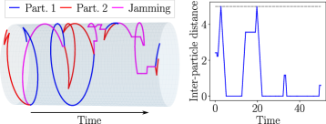
Figure 1: Trajectory of two RTPs undergoing instantaneous tumble (left), and of their corresponding periodic interdistance (right) ($\omega=0.2$, $L=10$).

We now characterize the stochastic dynamics of $r_{t}$ by a PDMP [31, 32], which is entirely encoded:

(a) by its infinitesimal generator in the bulk, $0<r_{t}<L/2$,

$$\mathcal{A}_{\mathcal{B}}\!=\!\underbrace{\nu\phi(s)\partial_{r}}_{\text{Run phase}}+\underbrace{\tilde{\omega}(s)(Q((\nu,s),\cdot)-\text{Id})}_{\text{Tumble phase}},$$ (1)

where we introduce the two auxiliary dynamical variables $(\nu_{t},s_{t})\in\mathcal{V}$ (so that the complete bulk set is $\mathcal{B}=]0,L/2[\times\mathcal{V}$): The variable $\nu_{t}\in\{-1,0,1\}$ sets the nature of the regime as defined in (a) and $\mathcal{V}$ can be decomposed as $\mathcal{V}_{-1}\cup\mathcal{V}_{0}\cup\mathcal{V}_{1}$. The variable $s_{t}=\{v_{t,1},v_{t,2}\}$, encoding the particle indistinguishability, sets the amplitude of the evolution by $\phi(s_{t})=|v_{t,1}-v_{t,2}|$ and the tumble by its rate $\tilde{\omega}(s_{t})=\omega(v_{t,1})+\omega(v_{t,2})$ and its transition Markov kernel $Q((\nu,s),\cdot)$,

$$\begin{split}Q((\nu,\{v,\tilde{v}\}),(\nu^{\prime},\{v^{\prime},\tilde{v}\}))\!=\!q(v,v^{\prime})\big{(}\tfrac{1}{2}\mathbb{1}_{\{0\}}(\nu)\mathbb{1}_{\{-1,1\}}(\nu^{\prime})\\ \ +\tfrac{\omega(v)}{\tilde{\omega}(\{v,\tilde{v}\})}\mathbb{1}_{\{-1,1\}}(\nu)\mathbb{1}_{\{\text{sign}(\nu\nu^{\prime})\}}\big{(}\text{sign}\big{(}\tfrac{v^{\prime}-\tilde{v}}{v-\tilde{v}}\big{)}\big{)}\big{)},\end{split}$$

all other transitions being of probability 0, as they would involve tumble of both particles. Thus, the particle indistinguishability leads to an isotropic symmetry for $Q$,

$$Q((\nu,s),(\nu^{\prime},s^{\prime}))=Q((-\nu,s),(-\nu^{\prime},s^{\prime})),$$ (2)

as illustrated on Fig. 2 for the instantaneous and finite tumbles. The symmetry (2) will have an important impact on the possible invariant distributions and justifies the introduction of the representation $(\nu,s)$.

Figure 2: Transitions between the internal states at the single particle (left) and interdistance level (right) in the case of instantaneous (top, and finite tumble (left), in a reduced representation for $s$ thanks to the single-particle tumble isotropy (instantaneous: $s$ can be omitted, finite: $s$ codes for the number of moving particles).

(b) by its behavior at the periodic boundary: at $(r,\nu,s)\in\{L/2\}\times\mathcal{V}_{1}=\Gamma^{*}_{P}$, the periodic boundary kernel $Q_{P}((r,\nu,s),(r^{\prime},\nu^{\prime},s^{\prime}))=\mathbb{1}_{\{(r,-\nu,s)\}}(r^{\prime},\nu^{\prime},s^{\prime})$ codes for a switch from an increasing ($\nu=1$) to a decreasing ($\nu^{\prime}=-1$) regime.

(c) and finally by its behavior at the jamming boundary: for $(r,\nu,s)\in\{0\}\times\mathcal{V}_{-1}=\Gamma^{*}_{J}$, the jamming boundary kernel, $Q_{J}((r,\nu,s),(r^{*},\nu^{*},s^{*}))=\mathbb{1}_{\{(r,\nu,s)\}}(r^{*},\nu^{*},s^{*})$ makes the system jumps into a jammed configuration $(r^{*},\nu^{*},s^{*})\in\mathcal{J}=\{0\}\times\mathcal{V}_{-1}\cup\mathcal{V}_{0}$, which is ruled by the following infinitesimal generator,

$$\mathcal{A}_{\mathcal{J}}\!=\!\tilde{\omega}(s^{*})(Q((\nu^{*},s^{*}),\cdot)-\text{Id}),$$ (3)

which translates the persistence of the jamming state until the tumbles lead to an unjamming state ($\nu=+1$), which, rigorously combined with an unjamming boundary kernel analogous to $Q_{\mathcal{J}}$, generates an increasing regime in the bulk.

II Conservation constraints in the steady state and jamming boundary role

The steady-state distribution of the periodic interdistance $r$ of two passive hardcore particles is the uniform density over $[0,L/2]$, with in particular a null probability to find $r$ in the exact state $0$. The addition of non-equilibrium features (activity, jamming) may introduce deviations from this equilibrium behavior, which we now study. The measure $\pi$ left invariant by the considered PDMP should satisfy the following condition,

$$\int_{\mathcal{B}}\mathcal{A}_{B}f(r,\nu,s)\textrm{d}\pi(r,\nu,s)+\int_{\mathcal{J}}\mathcal{A}_{J}f(0,\nu,s)\textrm{d}\pi(0,\nu,s)=0,$$ (4)

with $f$ a suitably smooth test function. As the considered process is trivially irreducible thanks to the ergodicity of the tumbles, the distribution $\pi$ is unique. Now, as $f$ can be any test function, we obtain by integration by part and boundary conditions, as detailed in Appendix A, the equivalent condition system,

$$\left\{\begin{array}[]{l}(\textrm{C}_{\mathcal{B}})\ \int_{\mathcal{V}}\pi(r,\textrm{d}\nu^{\prime}\textrm{d}s^{\prime})\tilde{\omega}(s^{\prime})Q((\nu^{\prime},s^{\prime}),(\nu,s))\\ \ \ \ \ =\tilde{\omega}(s)\pi(r,\nu,s)+\nu\phi(s)\partial_{r}\pi(r,\nu,s)\\ (\textrm{C}_{P})\ \pi(L/2,1,s)=\pi(L/2,-1,s)\\ (\textrm{C}_{\mathcal{J}})\ \int_{\mathcal{J}}\textrm{d}\pi(0,\nu^{\prime},s^{\prime})\tilde{\omega}(s^{\prime})Q((\nu^{\prime},s^{\prime}),(\nu,s))\\ \ \ \ \ =\mathbb{1}_{\{-1,0\}}(\nu)\tilde{\omega}(s)\pi(0,\nu,s)+\nu\phi(s)\pi(0^{+},\nu,s)\\ \end{array}\right.$$ (5)

This condition system completely constrains the invariant measure $\pi$. It can be understood as a set of conservation equations of probability flows in the bulk $\mathcal{B}$, and on the jamming and periodic boundaries. It leads to the following conclusions:

(i) $(\textrm{C}_{P})$ is a direct translation of the periodicity of the system and is not impacting the physical meaning of the form of $\pi$, in particular potential deviation from the passive equilibrium form.

(ii) In the bulk, $(\textrm{C}_{\mathcal{B}})$ is setting a balance between the Run and Tumble contributions. Any product measure of the form $\tfrac{2}{L}\mathbb{1}_{]0,L/2[}(r)\mu_{\mathcal{B}}(\cdot)$, with $\tilde{\omega}(\cdot)\mu_{\mathcal{B}}(\cdot)$ the unique invariant measure of the tumble kernel $Q$, is satisfying $(\textrm{C}_{B})$ with null Run term $\phi(\cdot)\partial_{r}\pi(r,\pm 1,\cdot)$. Furthermore, the isotropy of $Q$ (2) leads to $\mu_{\mathcal{B}}(\nu,s)=\mu_{\mathcal{B}}(-\nu,s)$, satisfying $(\textrm{C}_{P})$. Reciprocally, any distribution such that $\pi(r,\nu,s)=\pi(r,-\nu,s)$ is obeying $(\textrm{C}_{B})$ only if $\partial_{r}\pi=0$ for all $r>0$, i.e. only if $\tilde{\omega}(\cdot)\pi(\cdot)$ is invariant by $Q$ and then identifies with $\tilde{\omega}(\cdot)\mu_{\mathcal{B}}(\cdot)$.

(iii) The jamming condition $(\textrm{C}_{J})$ creates Dirac components in $r=0$ in $\pi$ for finite $\omega$, which are not present in the passive counterpart.

(iv) More interestingly, it appears clearly now that the jamming interaction can impact the bulk behavior by the term $\phi(s)\pi(0^{+},\pm 1,s)$ in $(\textrm{C}_{\mathcal{J}})$. It can be understood as a boundary source term for the bulk equation set by $(\textrm{C}_{\mathcal{B}})$, which can force the system away from the uniform distribution in $r$ in the bulk. This term comes from the integration by part, which stems from the Run term in $\mathcal{A}_{B}$. It is indeed the activity of the particles that pushes the exploration up to the boundary of the state space.

(v) In spite of the non-equilibrium features, we can derive some active global balance condition. Indeed, $(\textrm{C}_{\mathcal{J}})$ yields the global balance of the probability flows in and out of jamming, $\int\textrm{d}s\phi(s)\pi(0^{+},-1,s)=\int\textrm{d}s\phi(s)\pi(0^{+},1,s)$ and $(\textrm{C}_{B})$ imposes the global balance at any $r>0$ $\int\textrm{d}s\phi(s)\partial_{r}\pi(r,-1,s)=\int\textrm{d}s\phi(s)\partial_{r}\pi(r,1,s)$. Both combined, we obtain the following active global balance of the probability flows at any $r>0$,

$$\int\textrm{d}s\phi(s)\pi(r,-1,s)=\int\textrm{d}s\phi(s)\pi(r,1,s).$$ (6)

From (ii), any distribution $\pi$ obeying the stricter detailed counterpart of (6), i.e., for any $r,s$,

$$\pi(r,-1,s)=\pi(r,1,s),$$ (7)

must identify with $\tfrac{2}{L}\mathbb{1}_{]0,L/2[}(r)\mu_{\mathcal{B}}(\cdot)$ in the bulk. Actually, by symmetry argument, any distribution $\pi$ obeying (7) in at least a single point $r$ satisfies (7) in all $r$.

Thus, analyzing the conservation conditions in (5) unravels the potential impact of the non-equilibrium features on the invariant measure: First, the presence of Dirac terms in $r=0$ for finite $\omega$; Second, the deviation from a product measure uniform in $r$ in the bulk for unjamming scenarios which sets boundary conditions $\pi(0^{+},\cdot)$ different from the tumble stationary distribution $\mu_{\mathcal{B}}(\cdot)$.

III Universality classes and expression of the steady state

Therefore, we identify two universality classes, based on the deviation or not of $\pi(0^{+},\pm 1,s)$ from $\mu_{\mathcal{B}}(\pm 1,s)$, which can always be explicitly tested in $(C_{\mathcal{J}})$. It is equivalent to the satisfaction or breaking of the detailed symmetry upon entering and exiting jamming for any $s$,

$$\pi(0^{+},1,s)=\pi(0^{+},-1,s).$$ (8)

Detailed-jamming class. The detailed symmetry (8) is satisfied. As a consequence, the global-flow balance (6) condition is obeyed through the detailed-flow one (7) and the non-equilibrium nature is only apparent through the presence of Dirac term at the jamming point in the invariant distribution $\pi_{\textrm{det}}(r,\nu,s)$, which is of the form,

$$w_{\mathcal{J}}\mathbb{1}_{\{0\}}(r)\mu_{\mathcal{J}}(\nu,s)+w_{\mathcal{B}}\tfrac{2}{L}\mathbb{1}_{]0,L/2[}(r)\mu_{\mathcal{B}}(\nu,s),$$ (9)

with $\mu_{\mathcal{J}}$ the invariant jamming distribution and $w_{\mathcal{J}},w_{\mathcal{B}}$ the average time ratio respectively spent in jamming and the bulk, details on their derivation can be found in Appendix B. Very close to an equilibrium counterpart, it follows in the bulk a product form, which, once marginalized over the dynamical variables, identifies with the passive uniform steady-state. In particular, this is the case of the instantaneous tumble [26] but also of any systems with only two internal states $\pm v$.

Global-jamming class. The detailed symmetry (8) is not satisfied. This is for instance the case when the particles unjam at the smallest possible velocity when they jam together at different ones, implying some energy dissipation. This class then gathers systems further away from equilibrium, as we now explain. First, while the global-flow balance (6) still holds, there is no detailed-flow balance (7) at any point $r>0$ but at the periodic boundary $r=L/2$. Sign of a stronger non-equilibrium nature, the stationary distribution $\pi_{\text{glob}}(r,\nu,s)$ cannot longer be put under the form of Dirac contributions in $r=0$ and a product form in the bulk $r>0$, and writes itself,

$$w_{\mathcal{J}}\mathbb{1}_{\{0\}}(r)\mu_{\mathcal{J}}(\nu,s)+w_{\mathcal{B}}\tfrac{2}{L}\mathbb{1}_{]0,L/2[}(r)\mu(r,\nu,s),$$ (10)

where $\mu(r,\nu,s)\!=\!w_{\text{eq}}\mu_{\mathcal{B}}(\nu,s)\!+\!w_{\text{rel}}\gamma(r,\nu,s)$ and $\gamma(\cdot)$ stands for the relaxation in the bulk from the non-detailed constraint on its jamming boundary to the detailed constraint on its periodic one. Supposing that the internal states are of discrete values and as detailed in Appendix C.1, the bulk condition $(C_{\mathcal{B}})$ gives that $(\gamma(r,0,s))_{s}$ is determined by the sum of $\bm{\gamma}_{\pm}(r)=(\gamma(r,\pm 1,s))_{s}$, which obeys some relaxation equation,

$$\partial_{r}(\bm{\gamma}_{+}(r),\bm{\gamma_{-}}(r))=B(\bm{\gamma}_{+}(r),\bm{\gamma_{-}}(r)),$$ (11)

where, by the symmetry (2), the bulk matrix $B$ is of the form $B=\left(\begin{array}[]{cc}B^{+}&B^{-}\\ -B^{-}&-B^{+}\end{array}\right)$, leading to the uncoupled second-order system,

$$\left\{\begin{array}[]{l}\partial^{2}_{r}(\bm{\gamma}_{+}\!+\!\bm{\gamma}_{-})=(B^{+}\!-\!B^{-})(B^{+}\!+\!B^{-})(\bm{\gamma}_{+}\!+\!\bm{\gamma}_{-})\\ \partial^{2}_{r}(\bm{\gamma}_{+}\!-\!\bm{\gamma}_{-})=(B^{+}\!+\!B^{-})(B^{+}\!-\!B^{-})(\bm{\gamma}_{+}\!-\!\bm{\gamma}_{-})\end{array}\right.$$ (12)

The symmetry (2) also constrains the Jordan form of $B$, as it admits as eigenvalues symmetrical finite $(\pm\lambda_{k})_{k}$ of respective eigenvectors $(\bm{\mu}^{\pm}_{k,1},\bm{\mu}^{\mp}_{k,1})$ and necessarily $0$ of eigenvector $(\bm{\mu}_{\mathcal{B}},\bm{\mu}_{\mathcal{B}})$, see Appendix C.2.

The general solution of (11), whose precise expression is in Appendix C.3, derives from the spectral properties of $B$ and decomposes over a sum of exponentials of rate $(\pm\lambda_{k})_{k}$, modulated by polynomial terms stemming from possible degeneracies of the $\lambda_{k}$ and the boundary conditions. As $B$ admits $0$ as an eigenvalue, the general solution also admits a pure polynomial term.

An interesting case is when $B$ does not admit Jordan blocks of size bigger than $3$, as, from $(C_{P})$, any polynomial decay disappears and we recover an exact symmetry between decaying and increasing exponentials and such for any jamming scenario, leading to,

$$\begin{array}[]{r}\bm{\gamma}^{\pm}(r)\!=\!\sum_{k}a_{k}\Big{[}\cosh\left(\lambda_{k}\left(\frac{L}{2}\!-\!r\right)\right)\par(\bm{\mu}_{k,1}^{+}\!+\!\bm{\mu}_{k,1}^{-})\\ \!\mp\sinh\left(\lambda_{k}\left(\frac{L}{2}\!-\!r\right)\right)(\bm{\mu}_{k,1}^{+}\!-\!\bm{\mu}_{k,1}^{-})\Big{]},\end{array}$$ (13)

with $(a_{k})_{k}$ set by $(C_{\mathcal{J}})$. It yields a catenary-like relaxation once marginalized over $(\nu,s)$, as hinted by (12). A particular case is any system with particle internal states symmetrical enough so that $B$ only admits a single non-null $\pm\lambda_{k}$, so that $\lambda_{k}^{2}\propto\text{Tr}((B^{+}+B^{-})(B^{+}-B^{-}))$, as for the finite tumble (see Appendix C.4), which simplifies the formula in [27].

IV Discussion

The approach presented here gives a direct continuous-time and continuous-space setting, which encodes the fundamental system symmetries (periodicity, particle indistinguishability). By adequately capturing the jamming behavior as some boundary effect on the bulk, we are able to define the two universality classes of the steady-state behavior for systems of two RTPs with homogeneous tumbles. Interestingly, they are entirely defined from the satisfaction or not of a detailed symmetry (8) at the jamming point, which translates in the bulk into the satisfaction of the necessary active global balance (6) in a stricter –and closer to equilibrium– detailed manner (7) or not. Then, the further away from the detailed symmetry (8) the jamming scenario constrains the system, the more involved structure and relaxation behavior set by (11) are eventually exhibited in the bulk, see Appendix C.3.3. Indeed, the system is analogous to a catenary problem, where the active global balance acts as the fixed-length constraint on a cable or equivalently the RTP activity acts as some tension, while the tumble process acts as a weight force.

Thus, the impact of the time-reversibility breaking by the particle activity simply translates itself into the capacity of the system to explore its boundaries. There, the now seen jamming interactions may further impact the steady state, depending on some symmetry preservation. It is indeed reminiscent of the situation in non-reversible sampling by ECMC, where particle collisions can also be understood as infinite-rate jamming preserving some key symmetries.

The presented conclusions straightforwardly generalize into more general jamming scenario $\mathcal{A}_{J}$, set by some tumbling rates and kernel different from the bulk, as it only impacts the exact form of $w_{\mathcal{J}}$ and $\mu_{\mathcal{J}}(\cdot)$. Some future work lies in the study of the impact of non-homogeneity, with the tumbling depending on the RTP positions, as in presence of an external potential or soft interactions. The question of the relaxation of the system to its steady state should also find in the PDMP formalism a powerful approach that should be explored. More importantly, a compelling research perspective lies in the use of PDMPs and their faculty to isolate the impacts of boundary effects on the bulk to model more than two RTPs with hardcore jamming interactions. An explicit formula or a good quantitative understanding of the invariant measure would provide a new perspective on clustering phenomena such as MIPS, with a direct understanding of the impact of the microscopic details.

Supplementary Materials
Jamming pair of general run-and-tumble particles:
Exact results and universality classes

Appendix A Derivation of the system of conservation conditions

Piecewise deterministic Markov processes (PDMP) have been introduced in [31, 32]. A PDMP refers to a Markov process which evolves ballistically according to a deterministic differential flow, until a jump following some Poisson process occurs or the process reaches the domain boundary. We consider the PDMP defined by the infinitesimal generators $\mathcal{A}_{\mathcal{B}}$ and $\mathcal{A}_{\mathcal{J}}$ and by the periodic and jamming boundaries, as defined in (a), (b), (c).

The generator is an efficient tool to study the invariance of a measure $\pi$ (e.g. [32, Prop. 34.7]), as done in [35] for PDMP generated in particle systems by ECMC methods. The measure $\pi$ is indeed left invariant by the considered PDMP if the following condition is satisfied,

$$\int_{\mathcal{B}}\mathcal{A}_{B}f(r,\nu,s)\textrm{d}\pi(r,\nu,s)+\int_{\mathcal{J}}\mathcal{A}_{J}f(0,\nu,s)\textrm{d}\pi(0,\nu,s)=0,$$ (14)

with $f$ a suitably smooth test function (here we do not detail the description of the extended domain of the generator and a suitable core, as required by [32, Th. 5.5, ]). Furthermore, stemming from the periodic boundary kernel $Q_{P}$, $f$ shall verify the condition on the periodic boundary,

$$f(L/2,\nu,s)=f(L/2,-\nu,s).$$ (15)

Similar conditions at the jamming boundary are required, i.e.

$$f(0^{+},\nu,s)=f(0,\nu,s),$$ (16)

where we omit out of simplicity the superscript ^∗ characterizing the jamming state. Now, expliciting the bulk term in 14,

$$\begin{split}\int_{\mathcal{V}_{-1}\cup\mathcal{V}_{0}}\mathcal{A}_{J}f(0,\nu,s)\pi(0,d\nu,ds)+\int_{]0,L/2[\times\mathcal{V}}\textrm{d}\pi(r,\nu,s)\nu\phi(s)\partial_{r}f(r,\nu,s)\\ +\int_{]0,L/2[\times\mathcal{V}}\textrm{d}\pi(r,\nu,s)\tilde{\omega}(s)\int_{\mathcal{V}}Q((\nu,s),(\textrm{d}\nu^{\prime}\textrm{d}s^{\prime}))\Big{(}f(r,\nu^{\prime},s^{\prime})-f(r,\nu,s)\Big{)}=0,\end{split}$$ (17)

we obtain by integration by parts in the second term,

$$\begin{split}\int_{\mathcal{V}_{-1}\cup\mathcal{V}_{0}}\mathcal{A}_{J}f(0,\nu,s)\pi(0,\textrm{d}\nu,\textrm{d}s)-\int_{\mathcal{V}_{-1}\cup\mathcal{V}_{1}}\nu\phi(s)\pi(0^{+},\textrm{d}\nu,\textrm{d}s)f(0,\nu,s)+\int_{\mathcal{V}_{-1}\cup\mathcal{V}_{1}}\nu\phi(s)\pi(L/2^{-},\textrm{d}\nu,\textrm{d}s)f(L/2,\nu,s)\\ +\int_{]0,L/2[\times\mathcal{V}}\textrm{d}r\textrm{d}\nu\textrm{d}sf(r,\nu,s)\Big{[}\int_{\mathcal{V}}\pi(r,\textrm{d}\nu^{\prime},\textrm{d}s^{\prime})\tilde{\omega}(s^{\prime})Q((\nu^{\prime},s^{\prime}),(\nu,s))-\pi(r,\nu,s)\tilde{\omega}(s)-\nu\phi(s)\partial_{r}\pi(r,\nu,s)\Big{]}=0.\end{split}$$ (18)

As, $f(L/2,\nu,s)=f(L/2,-\nu,s)$ by the condition on the periodic boundary, $\pi(L/2,-\nu,s)=\pi(L/2,\nu,s)$ by definition of the periodic interdistance, we have the cancellation of the term in $L/2$ by periodicity,

$$\int_{\mathcal{V}_{1}}\nu\phi(s)\pi(L/2,\textrm{d}\nu,\textrm{d}s)f(L/2,\nu,s)+\int_{\mathcal{V}_{-1}}-(-\nu)\phi(s)\pi(L/2,-\textrm{d}\nu,\textrm{d}s)f(L/2,-\nu,s)=0.$$ (19)

Thus we have, expliciting the jamming generator,

$$\begin{split}\int_{\mathcal{V}}\textrm{d}\nu\textrm{d}sf(0,\nu,s)\Big{[}\int_{\mathcal{V}_{-1}\cup\mathcal{V}_{0}}\pi(0,\textrm{d}\nu^{\prime},\textrm{d}s^{\prime})\tilde{\omega}(s^{\prime})Q((\nu^{\prime},s^{\prime}),(\nu,s))-\mathbb{1}_{\{-1,0\}}(\nu)\pi(0,\nu,s)\tilde{\omega}(s)-\nu\phi(s)\pi(0^{+},\nu,s)\Big{]}\\ +\int_{]0,L/2[\times\mathcal{V}}\textrm{d}r\textrm{d}\nu\textrm{d}sf(r,\nu,s)\Big{[}\int_{\mathcal{V}}\pi(r,\textrm{d}\nu^{\prime},\textrm{d}s^{\prime})\tilde{\omega}(s^{\prime})Q((\nu^{\prime},s^{\prime}),(\nu,s))-\pi(r,\nu,s)\tilde{\omega}(s)-\nu\phi(s)\partial_{r}\pi(r,\nu,s))\Big{]}\\ =0.\end{split}$$ (20)

As $f$ can be any test function and recalling the periodic condition, we obtain the following equivalent condition system,

$$\left\{\begin{array}[]{ll}(\textrm{C}_{B})&\int_{\mathcal{V}}\pi(r,\textrm{d}\nu,\textrm{d}s^{\prime})\tilde{\omega}(s^{\prime})Q((\nu^{\prime},s^{\prime}),(\nu,s))=\pi(r,\nu,s)\tilde{\omega}(s)+\nu\phi(s)\partial_{r}\pi(r,\nu,s)\text{ for any }(r,\nu,s)\in\mathcal{B},\\ (\textrm{C}_{P})&\pi(L/2,1,s)=\pi(L/2,-1,s)\text{ for any }(\pm 1,s)\in\mathcal{V}_{\pm 1},\\ (\textrm{C}_{J})&\int_{\mathcal{V}_{-1}\cup\mathcal{V}_{0}}\pi(0,\textrm{d}\nu^{\prime}\textrm{d}s^{\prime})\tilde{\omega}(s^{\prime})Q((\nu^{\prime},s^{\prime}),(\nu,s))=\mathbb{1}_{\{-1,0\}}(\nu)\pi(0,\nu,s)\tilde{\omega}(s)+\nu\phi(s)\pi(0^{+},\nu,s)\text{ for any }(\nu,s)\in\mathcal{V}\end{array}\right.,$$ (21)

which identifies with the system (5), whose consequences are further discussed in Section II.

Appendix B Derivation of the detailed-jamming steady state

We now determine in more details the steady-state distribution in the detailed-jamming class as introduced in (9) in Section III and as recalled here,

$$\pi_{\textrm{det}}(r,\nu,s)=w_{\mathcal{J}}\mathbb{1}_{\{0\}}(r)\mu_{\mathcal{J}}(\nu,s)+w_{\mathcal{B}}\tfrac{2}{L}\mathbb{1}_{]0,L/2[}(r)\mu_{\mathcal{B}}(\nu,s).$$

Plugging the detailed-jamming symmetry (8) into $(\textrm{C}_{J})$ (5), we obtain,

$$\int_{\mathcal{V}_{-1}\cup\mathcal{V}_{0}}\textrm{d}\mu_{\mathcal{J}}(\nu^{\prime},s^{\prime})\tilde{\omega}(s^{\prime})Q((\nu^{\prime},s^{\prime}),(1,s))=\phi(s)\pi(0^{+},1,s)=-(-1)\phi(s)\pi(0^{+},-1,s),$$

and derive an explicit condition on the jamming equivalent to (8) ,

$$(\textrm{C}_{\textrm{det}})\left\{\begin{array}[]{l}\int_{\mathcal{V}_{-1}\cup\mathcal{V}_{0}}\textrm{d}\mu_{\mathcal{J}}(\nu^{\prime},s^{\prime})\tilde{\omega}(s^{\prime})Q((\nu^{\prime},s^{\prime}),(0,s))=\tilde{\omega}(s)\mu_{\mathcal{J}}(0,s)\\ \int_{\mathcal{V}_{-1}\cup\mathcal{V}_{0}}\textrm{d}\mu_{\mathcal{J}}(\nu^{\prime},s^{\prime})\tilde{\omega}(s^{\prime})(Q((\nu^{\prime},s^{\prime}),(-1,s))+Q((\nu^{\prime},s^{\prime}),(1,s)))=\tilde{\omega}(s)\mu_{\mathcal{J}}(-1,s)\\ \int_{\mathcal{V}_{-1}\cup\mathcal{V}_{0}}w_{\mathcal{J}}\textrm{d}\mu_{\mathcal{J}}(\nu^{\prime},s^{\prime})\tilde{\omega}(s^{\prime})Q((\nu^{\prime},s^{\prime}),(1,s))=\phi(s)w_{\mathcal{B}}\tfrac{2}{L}\mu_{\mathcal{B}}(1,s)\ \text{for any}\ (1,s)\in\mathcal{V}_{1}\end{array}\right.,$$ (22)

so that the jamming invariant measure $\mu_{\mathcal{J}}$ is completely characterized by the first two lines and only depends on the jamming scenario. Then, the ratio $w_{\mathcal{J}}/w_{\mathcal{B}}$ of time spent respectively while jamming and in the bulk is set by the last line. The ratio $w_{\mathcal{J}}/w_{\mathcal{B}}$ does not depend on $s$ as the jamming exit probability in state $(1,s)$ (left term of the last line) is indeed proportional to the invariant bulk probability $\mu_{\mathcal{B}}(\pm 1,s)$ of this state, which is known from $(C_{\mathcal{B}})$, as we recall,

$$\int_{\mathcal{V}}\mu_{\mathcal{B}}(\textrm{d}\nu^{\prime}\textrm{d}s^{\prime})\tilde{\omega}(s^{\prime})Q((\nu^{\prime},s^{\prime}),\textrm{d}\nu\textrm{d}s)=\mu_{\mathcal{B}}(\textrm{d}\nu,\textrm{d}s)\tilde{\omega}(s).$$

An interesting particular case is systems with two internal states $v_{1},v_{2}$, which includes the case of the instantaneous tumble ($v_{1},v_{2}=-1,+1$, $\omega(v_{1})=\omega(v_{2})$), as illustrated in Figure 2. These systems are always detailed-jamming ones, as there is only one entry state into jamming and one exit state out of jamming, realizing the detailed-jamming symmetry (8). For these systems, we obtain,

$$(\textrm{C}_{\textrm{det}})\left\{\begin{array}[]{l}\mu_{\mathcal{J}}(-1,\{v_{1},v_{2}\})\omega(v_{1})=2\omega(v_{2})\mu_{\mathcal{J}}(0,\{v_{2},v_{2}\})\\ \mu_{\mathcal{J}}(-1,\{v_{1},v_{2}\})\omega(v_{2})=2\omega(v_{1})\mu_{\mathcal{J}}(0,\{v_{1},v_{1}\})\\ w_{\mathcal{J}}\omega(v_{1})\mu_{\mathcal{J}}(0,\{v_{1},v_{1}\})+w_{\mathcal{J}}\omega(v_{2})\mu_{\mathcal{J}}(0,\{v_{2},v_{2}\})=w_{\mathcal{B}}\tfrac{2|v_{1}-v_{2}|}{L}\mu_{\mathcal{B}}(1,\{v_{1},v_{2}\})\\ \iff\tfrac{1}{2}w_{\mathcal{J}}(\omega(v_{1})+\omega(v_{2}))\mu_{\mathcal{J}}(-1,\{v_{1},v_{2}\})=w_{\mathcal{B}}\tfrac{2|v_{1}-v_{2}|}{L}\mu_{\mathcal{B}}(1,\{v_{1},v_{2}\})\end{array}\right.,$$ (23)

and,

$$\left\{\begin{array}[]{l}\omega(v_{2})\mu_{\mathcal{B}}(\pm 1,\{v_{1},v_{2}\})=\omega(v_{1})\mu_{\mathcal{B}}(0,\{v_{1},v_{1}\})\\ \omega(v_{1})\mu_{\mathcal{B}}(\pm 1,\{v_{1},v_{2}\})=\omega(v_{2})\mu_{\mathcal{B}}(0,\{v_{2},v_{2}\})\\ \end{array}\right..$$

We then get,

$$\begin{array}[]{lllll}\left\{\begin{array}[]{l}\mu_{\mathcal{J}}(0,\{v_{1},v_{1}\})=\tfrac{\omega(v_{2})^{2}}{\mathcal{N}_{\mathcal{J}}}\\ \mu_{\mathcal{J}}(0,\{v_{2},v_{2}\})=\tfrac{\omega(v_{1})^{2}}{\mathcal{N}_{\mathcal{J}}}\\ \mu_{\mathcal{J}}(-1,\{v_{1},v_{2}\})=2\tfrac{\omega(v_{1})\omega(v_{2})}{\mathcal{N}_{\mathcal{J}}}\\ \mathcal{N}_{\mathcal{J}}=\big{(}\omega(v_{1})+\omega(v_{2})\big{)}^{2}\end{array}\right.,&&\left\{\begin{array}[]{l}\mu_{\mathcal{B}}(0,\{v_{1},v_{1}\})=\tfrac{\omega(v_{2})^{2}}{\mathcal{N}_{\mathcal{B}}}\\ \mu_{\mathcal{B}}(0,\{v_{2},v_{2}\})=\tfrac{\omega(v_{1})^{2}}{\mathcal{N}_{\mathcal{B}}}\\ \mu_{\mathcal{B}}(\pm 1,\{v_{1},v_{2}\})=\tfrac{\omega(v_{1})\omega(v_{2})}{\mathcal{N}_{\mathcal{B}}}\\ \mathcal{N}_{\mathcal{B}}=\big{(}\omega(v_{1})+\omega(v_{2})\big{)}^{2}\end{array}\right.&\text{ and }&\left\{\begin{array}[]{l}w_{\mathcal{B}}=\frac{1}{1+\tfrac{2|v_{1}-v_{2}|}{L(\omega(v_{1})+\omega(v_{2}))}}\\ w_{\mathcal{J}}/w_{\mathcal{B}}=\tfrac{2|v_{1}-v_{2}|}{L(\omega(v_{1})+\omega(v_{2}))}\end{array}\right..\end{array}$$ (24)

where the ratio $w_{\mathcal{J}}/w_{\mathcal{B}}$ of time spent in jamming versus in the bulk increases with the strength of the ballistic nature of the considered RTP dynamics (decrease of the time needed to cover the length $L$ of the torus, decrease of the total tumble rate). Computations for systems with more than two internal states are similar. We finally also stress that the conditions determined here also applied for a continuous distribution of internal states.

Appendix C Derivation of the global-jamming steady state

We now determine in more details for discrete distributions of internal states the steady-state distribution in the global-jamming class as introduced in (10) in Section III and as recalled here,

$$\pi_{\textrm{glob}}(r,\nu,s)=w_{\mathcal{J}}\mathbb{1}_{\{0\}}(r)\mu_{\mathcal{J}}(\nu,s)+w_{\mathcal{B}}\tfrac{2}{L}\mathbb{1}_{]0,L/2[}(r)(w_{\text{eq}}\mu_{\mathcal{B}}(\nu,s)+w_{\text{rel}}\gamma(r,\nu,s)).$$

We do so by first deriving in Section C.1 the bulk relaxation equation, which is ruled by the bulk relaxation matrix $B$. We then study in Section C.2 the spectral properties of $B$, which are strongly constrained by the symmetry (2) of $Q$. We then obtain a general explicit expression for $\gamma(\cdot)$ in Section C.3, which we completely determine in particular cases including the finite tumble in Section C.4.

C.1 Bulk evolution equation

We obtain, by plugging $\pi_{\textrm{glob}}$ into the bulk condition $(C_{\mathcal{B}})$ and exploiting the symmetry (2) of $Q$,

$$\left\{\begin{array}[]{rl}\gamma(r,0,s)\tilde{\omega}(s)=&\int\textrm{d}s^{\prime}\mathbb{1}_{\mathcal{V}_{1}}((1,s^{\prime}))(\gamma(r,-1,s^{\prime})+\gamma(r,1,s^{\prime}))\tilde{\omega}(s^{\prime})Q((1,s^{\prime}),(0,s))\\ \pm\partial_{r}\gamma(r,\pm 1,s)=&-\phi(s)^{-1}\gamma(r,\pm 1,s)\tilde{\omega}(s)\\ &+\phi(s)^{-1}\int\textrm{d}s^{\prime}\mathbb{1}_{\mathcal{V}_{1}}((1,s^{\prime}))\Big{[}\gamma(r,1,s^{\prime})Q((1,s^{\prime}),(\pm 1,s))+\gamma(r,-1,s^{\prime})Q((-1,s^{\prime}),(\pm 1,s))\\ &+(\gamma(r,1,s^{\prime})+\gamma(r,-1,s^{\prime}))\int\textrm{d}s^{\prime\prime}\mathbb{1}_{\mathcal{V}_{0}}((0,s^{\prime\prime}))Q((1,s^{\prime}),(0,s^{\prime\prime}))Q((0,s^{\prime\prime}),(1,s))\Big{]}\tilde{\omega}(s^{\prime})\end{array}\right.$$ (25)

We note,

$$\bm{\gamma}(r)=\left(\begin{array}[]{l}\bm{\gamma}^{+}(r)=(\gamma(1,s))_{(1,s)\in\mathcal{V}_{1}}\\ \bm{\gamma}^{-}(r)=(\gamma(\!-\!1,s))_{(-1,s)\in\mathcal{V}_{-1}}\end{array}\right).$$

and summarize (25) into,

$$\partial_{r}\bm{\gamma}(r)=B\bm{\gamma}$$ (26)

with $B$ the bulk relaxation matrix,

$$B=\left(\begin{array}[]{cc}B^{+}&B^{-}\\ -B^{-}&-B^{+}\end{array}\right)\in M_{2|\mathcal{V}_{1}|\times 2|\mathcal{V}_{1}|}(\mathbb{R})$$ (27)

and,

$$B^{+}=D^{-1}_{\phi}(Q^{+}-I)D_{\omega},\ \ B^{-}=D^{-1}_{\phi}Q^{-}D_{\omega}\in M_{|\mathcal{V}_{1}|\times\mathcal{V}_{1}|}(\mathbb{R})$$ (28)

$$D_{\phi,ss^{\prime}}=\phi(s)\delta_{ss^{\prime}}\ \text{and}\ D_{\omega,ss^{\prime}}=\omega(s)\delta_{ss^{\prime}},$$ (29)

and,

$$Q^{\pm}_{ss^{\prime}}=Q((\pm 1,s^{\prime}),(1,\textrm{d}s))+\sum_{s^{\prime\prime}}Q((\pm 1,s^{\prime}),(0,\textrm{d}s^{\prime\prime}))Q((0,s^{\prime\prime}),(1,\textrm{d}s)).$$ (30)

As $Q$ is a Markov kernel and as there is no tumble between two states with $\nu=0$ since it will require a tumble of each particle at the same time, we have for any $(1,s^{\prime})\in\mathcal{V}_{1}$ the conservation identity,

$$\sum_{s}(Q^{+}_{ss^{\prime}}+Q^{-}_{ss^{\prime}}-\delta_{ss^{\prime}})=0$$ (31)

i.e.,

$$\sum_{s}\phi(s)\big{(}B^{+}+B^{-}\big{)}_{ss^{\prime}}=0,$$ (32)

which is consistent with the active global balance condition (6), as clearly appearing when rewritten as,

$$\sum_{s}\phi(s)(\partial_{r}\bm{\gamma}_{s}^{+}(r)-\partial_{r}\bm{\gamma}_{s}^{-}(r))=0=\sum_{s}\phi(s)\big{(}B^{+}+B^{-}\big{)}_{ss^{\prime}}(\bm{\gamma}_{s^{\prime}}^{+}(r)+\bm{\gamma}_{s^{\prime}}^{-}(r)).$$ (33)

C.2 Spectral analysis of bulk matrix $B$

C.2.1 Jordan reduction of $B$ and symmetry constraints

We now consider the Jordan reduction of $B=P^{-1}JP$, with $J$ a Jordan matrix. For the Jordan block $k$ of size $p_{k}$, we note the corresponding eigenvalue $\lambda_{k}$ and the Jordan chain of linearly-independent generalized eigenvectors $\bm{\mu_{k,n}}=(\bm{\mu}^{+}_{k,n},\bm{\mu}^{-}_{k,n})$, with $1\leq n\leq p_{k}$, $\bm{\mu_{k,1}}$ being an eigenvector and $B\bm{\mu}_{k,n}=\lambda_{k}\bm{\mu}_{k,n}+\bm{\mu}_{k,n-1}$ for $n>1$.

By the symmetry of $B$, any block $k$ of eigenvalue $\lambda_{k}>0$ is mirrored by a block $k^{*}$ of eigenvalue $\lambda_{k^{*}}=-\lambda_{k}$ and generalized eigenvectors $\bm{\mu}_{k^{*},n}=(-1)^{n+1}(\bm{\mu}^{-}_{k,n},\bm{\mu}^{+}_{k,n})$, as $B(\bm{\mu}^{-}_{k,1},\bm{\mu}^{+}_{k,1})=-\lambda_{k}(\bm{\mu}^{-}_{k,1},\bm{\mu}^{+}_{k,1})$ and, for $n>1$,

$$(-1)^{n+1}B(\bm{\mu}^{-}_{k,n},\bm{\mu}^{+}_{k,n})=-\lambda_{k}(-1)^{n+1}(\bm{\mu}^{-}_{k,n},\bm{\mu}^{+}_{k,n})+(-1)^{n}(\bm{\mu}^{-}_{k,n-1},\bm{\mu}^{+}_{k,n-1}).$$

Furthermore, as $\hat{D}^{\pm}_{\phi}B\hat{D}^{-1}_{\omega}$, with $\hat{D}^{\pm}_{\phi}=\left(\begin{smallmatrix}D_{\phi}&0\\ 0&-D_{\phi}\\ \end{smallmatrix}\right)$ and $\hat{D}^{-1}_{\omega}=\left(\begin{smallmatrix}D^{-1}_{\omega}&0\\ 0&D^{-1}_{\omega}\\ \end{smallmatrix}\right)$ , identifies with the tumble Markov kernel collapsed in $\nu=0$ of the considered process, it is diagonalizable with real eigenvalues ranging from $0$ to $-1$ and a unique eigenvector $\bm{\mu}$ so that $\hat{D}^{\pm}_{\phi}B\hat{D}^{-1}_{\omega}\bm{\mu}=0$. The vector $\bm{\mu}$ identifies with the unique stationary bulk solution as $\bm{\mu}=\hat{D}_{\omega}(\bm{\mu}_{\mathcal{B}},\bm{\mu}_{\mathcal{B}})$. As $\hat{D}_{\phi}$ is invertible, $(\bm{\mu}_{\mathcal{B}},\bm{\mu}_{\mathcal{B}})$ is the unique eigenvector of eigenvalue $0$ of $B$. Then, for the unique block $k$ with $\lambda_{k}=0$, the generalized eigenvectors are of the following form $\bm{\mu_{k,n}}=(\bm{\mu}^{+}_{k,n},(-1)^{n+1}\bm{\mu}^{+}_{k,n})$, as,

$$\left\{\begin{array}[]{l}\bm{\mu}_{k,1}=(\bm{\mu}_{\mathcal{B}},\bm{\mu}_{\mathcal{B}})\\ B\bm{\mu}_{k,n}=\bm{\mu}_{k,n-1},\ n>1\end{array}\right.\ \ \text{gives}\ \ \left\{\begin{array}[]{ll}(B^{+}+(-1)^{n+1}B^{-})\bm{\mu}^{+}_{k,n}&=\bm{\mu}^{+}_{k,n-1}\\ -((-1)^{n+1}B^{+}+B^{-})\bm{\mu}^{+}_{k,n}&=(-1)^{n}\bm{\mu}^{+}_{k,n-1}\\ \end{array}\right.$$

It is finally noteworthy that $(\bm{\mu}_{\mathcal{B}},\bm{\mu}_{\mathcal{B}})$ is the only symmetrical eigenvector of $B$, as any symmetrical eigenvector is of eigenvalue $0$, as can be seen directly from $B$ or from an equivalent argument of linear independence for $\lambda_{k}\neq 0$ of the eigenvectors $(\bm{\mu}^{+}_{k,n},\bm{\mu}^{-}_{k,n})$ (e.v. $\lambda_{k}$) and $(\bm{\mu}^{-}_{k,n},\bm{\mu}^{+}_{k,n})$ (e.v. $-\lambda_{k}$). This is consistent with the fact that a symmetrical eigenvector is by definition a stationary solution of the detailed-jamming class which is unique and of eigenvalue $0$. Hence the complete characterization only by the detailed-symmetry condition ($\pi(r,\nu,s)=-\pi(r,-\nu,s)$) of the detailed-jamming class, which is equivalent to $\pi(r,\nu,s)=\mu_{Q}(\nu,s)$.

Thus, the number of Jordan blocks of $J$ is odd and is noted $2d+1$. We rank the blocks from $-d$ to $d$ in a symmetrical manner: The $k$-th block of eigenvalue $\lambda_{k}$ and generalized eigenvectors $(\bm{\mu}^{+}_{k,n},\bm{\mu}^{-}_{k,n})$ is mirrored by the $(-k)$-th block of eigenvalue $-\lambda_{k}$, generalized eigenvectors $((-1)^{n+1}\bm{\mu}^{-}_{k,n},(-1)^{n+1}\bm{\mu}^{+}_{k,n})$ . We then set the position of the block linked to the eigenvector $(\bm{\mu}_{0,1},\bm{\mu}_{0,1})=(\bm{\mu}_{\mathcal{B}},\bm{\mu}_{\mathcal{B}})$ to the $0$-th rank. It is composed of generalized eigenvectors of the form $(\bm{\mu}_{0,n},(-1)^{n+1}\bm{\mu}_{0,n})$.

It is noteworthy that, as $B$ is of even size, the Jordan block associated to $\lambda_{0}=0$ must be of an even size $p_{0}>0$, so that $B$ is never diagonalizable. This is a direct consequence of the symmetry imposed on $Q$ by the particle indistinguishability and space homogeneity.

C.2.2 Spectral relationship with submatrices $B_{+}$ and $B_{-}$ and catenary equation

The family $((\bm{\mu}^{+}_{k,n},\bm{\mu}^{-}_{k,n})_{k,n},(\bm{\mu}_{0,n},(-1)^{n+1}\bm{\mu}_{0,n})_{n},(\bm{\mu}^{-}_{k,n},\bm{\mu}^{+}_{k,n})_{k,n})$ naturally forms a basis of $\mathbb{R}^{2|\mathcal{V}_{1}|}$. Furthermore, the vectors $(\bm{\mu}^{+}_{k,n}+\bm{\mu}^{-}_{k,n})_{k,n}$ (resp. $(\bm{\mu}^{+}_{k,n}-\bm{\mu}^{-}_{k,n})_{k,n}$) are linearly independent. Indeed, if it exists $\{b_{k,n}\}$ so that $\sum_{k,n}b_{k,n}\bm{\mu}^{+}_{k,n}=-\sum_{k,n}b_{k,n}\bm{\mu}^{-}_{k,n}$ (resp. $=\sum_{k,n}b_{k,n}\bm{\mu}^{-}_{k,n}$), then we have $\sum_{k,n}b_{k,n}\bm{\mu}_{k,n}=-\sum_{k,n}b_{k,n}(-1)^{n+1}\bm{\mu}_{-k,n}$ (resp. $=\sum_{k,n}b_{k,n}\bm{\mu}_{k,n}$) , which is not possible. Eventually, by considering the size of the sets $(\bm{\mu}^{+}_{k,n}\pm\bm{\mu}^{-}_{k,n})$, they form two basis of $\mathbb{R}^{|\mathcal{V}_{1}|}$.

In addition, we have the relationships, noting $M^{+}=(B^{+}+B^{-})$ and $M^{-}=(B^{+}-B^{-})$,

$$\begin{aligned} \text{For $k>0$, }&\left\{\begin{array}[]{l}M^{+}(\bm{\mu}^{+}_{k,1}+\bm{\mu}^{-}_{k,1})=\lambda_{k}(\bm{\mu}^{+}_{k,1}-\bm{\mu}^{-}_{k,1})\\ M^{-}(\bm{\mu}^{+}_{k,1}-\bm{\mu}^{-}_{k,1})=\lambda_{k}(\bm{\mu}^{+}_{k,1}+\bm{\mu}^{-}_{k,1})\end{array}\right.&\text{and}&\left\{\begin{array}[]{l}M^{+}\bm{\mu}_{0,1}=0\\ M^{-}\bm{\mu}_{0,2}=\bm{\mu}_{0,1}\\ \end{array}\right.\end{aligned},$$ (34)

so that, the vectors $(\bm{\mu}^{+}_{k,1}\pm\bm{\mu}^{-}_{k,1})_{k>1}$ are respectively the eigenvectors of $M^{\mp}M^{\pm}$ of eigenvalues $\lambda_{k}^{2}$ and $\bm{\mu}_{0,1}$ (resp. $\bm{\mu}_{0,2}$) is the eigenvector of $M^{-}M^{+}$ (resp. $M^{+}M^{-}$) of eigenvalue $0$.

And furthermore, for $n>1$, we have,

$$\begin{aligned} \text{For $k>0$, }&\left\{\begin{array}[]{l}M^{+}(\bm{\mu}^{+}_{k,n}+\bm{\mu}^{-}_{k,n})=\lambda_{k}(\bm{\mu}^{+}_{k,n}-\bm{\mu}^{-}_{k,n})+(\bm{\mu}^{+}_{k,n-1}-\bm{\mu}^{-}_{k,n-1})\\ M^{-}(\bm{\mu}^{+}_{k,n}-\bm{\mu}^{-}_{k,n})=\lambda_{k}(\bm{\mu}^{+}_{k,n}+\bm{\mu}^{-}_{k,n})+(\bm{\mu}^{+}_{k,n-1}+\bm{\mu}^{-}_{k,n-1})\end{array}\right.&\text{and}&\left\{\begin{array}[]{l}M^{+}\bm{\mu}_{0,2n+1}=\bm{\mu}_{0,2n}\\ M^{-}\bm{\mu}_{0,2n}=\bm{\mu}_{0,2n-1}\\ \end{array}\right.\end{aligned}.$$ (35)

Giving, for $p<n$,

For $$k>0 \left\{\begin{array}[]{l}(M^{-}M^{+}-\lambda_{k}^{2})^{p}(\bm{\mu}^{+}_{k,n}+\bm{\mu}^{-}_{k,n})\neq\bm{0}\\ (M^{+}M^{-}-\lambda_{k}^{2})^{p}(\bm{\mu}^{+}_{k,n}-\bm{\mu}^{-}_{k,n})\neq\bm{0}\end{array}\right. \left\{\begin{array}[]{l}(M^{-}M^{+})^{p}\bm{\mu}_{0,2n+1}\neq\bm{0}\\ (M^{+}M^{-})^{p}\bm{\mu}_{0,2n}\neq\bm{0}\end{array}\right.$$, and (36)

For $$k>0 \left\{\begin{array}[]{l}(M^{-}M^{+}-\lambda_{k}^{2})^{n-1}(\bm{\mu}^{+}_{k,n}+\bm{\mu}^{-}_{k,n})=\bm{\mu}^{+}_{k,1}+\bm{\mu}^{-}_{k,1}\\ (M^{+}M^{-}-\lambda_{k}^{2})^{n-1}(\bm{\mu}^{+}_{k,n}-\bm{\mu}^{-}_{k,n})=\bm{\mu}^{+}_{k,1}-\bm{\mu}^{-}_{k,1}\end{array}\right. \left\{\begin{array}[]{l}(M^{-}M^{+})^{n-1}\bm{\mu}_{0,2n-1}=\bm{\mu}_{0,1}\\ (M^{+}M^{-})^{n-1}\bm{\mu}_{0,2n}=\bm{\mu}_{0,2},\end{array}\right.$$, and

so that, $((\bm{\mu}^{+}_{k,n}+\bm{\mu}^{-}_{k,n})_{k,1<n\leq p_{k}},(\bm{\mu}_{0,2n-1})_{1<n\leq p_{0}/2})$ (resp. $((\bm{\mu}^{+}_{k,n}-\bm{\mu}^{-}_{k,n})_{k,1<n\leq p_{k}},(\bm{\mu}_{0,2n})_{1<n\leq p_{0}/2})$) are generalized eigenvectors of $M^{-}M^{+}$ (resp. of $M^{+}M^{-}$).

More generally, the spectral properties of $B$ and $M^{+}M^{-}$, $M^{-}M^{+}$ are strongly related. Indeed, the characteristic polynomial of $B$ writes itself in terms of $B^{2}$, as,

$$B^{p_{0}}\prod_{k=1}^{d}(B-\lambda_{k}I)^{p_{k}}(B+\lambda_{k}I)^{p_{k}}=(B^{2})^{p_{0}/2}\prod_{k=1}^{d}(B^{2}-\lambda_{k}^{2}I)^{p_{k}} =0$$ (37)

$$B^{2(p_{0}/2)}\sum_{m=0}^{d}B^{2m}\sum_{\{i_{k}\}_{k=1}^{d-m}}\prod_{k=1}^{d-m}\lambda_{i_{k}}^{2} =0.$$

And, as,

$$B^{2m}=\frac{1}{2}\left(\begin{array}[]{cc}(M^{-}M^{+})^{m}+(M^{+}M^{-})^{m}&(M^{-}M^{+})^{m}-(M^{+}M^{-})^{m}\\ (M^{-}M^{+})^{m}-(M^{+}M^{-})^{m}&(M^{-}M^{+})^{m}+(M^{+}M^{-})^{m}\end{array}\right)$$

it is equivalent to,

$$\left\{\begin{array}[]{rl}(M^{+}M^{-})^{p_{0}/2}\sum_{m=0}^{d}(M^{+}M^{-})^{m}\sum_{\{i_{k}\}_{k=1}^{d-m}}\prod_{k=1}^{d-m}\lambda_{i_{k}}^{2}&=0\\ (M^{-}M^{+})^{p_{0}/2}\sum_{m=0}^{d}(M^{-}M^{+})^{m}\sum_{\{i_{k}\}_{k=1}^{d-m}}\prod_{k=1}^{d-m}\lambda_{i_{k}}^{2}&=0.\\ \end{array}\right.$$ (38)

So that, the characteristic polynomials of $M^{+}M^{-}$ and $M^{-}M^{+}$ are,

$$(M^{\pm}M^{\mp})^{p_{0}/2}\prod_{k=1}^{d}(M^{\pm}M^{\mp}-\lambda_{k}^{2}I)^{p_{k}}=0.\\$$ (39)

A similar derivation can be carried out regarding the minimal polynomial and, thus, the fact that $B$ admits no generalized eigenvectors apart the necessary $\bm{\mu}_{0,2}$ (i.e. $p_{0}=2$, $p_{k\neq 0}=1$) is equivalent to $M^{+}M^{-}$ and $M^{-}M^{+}$ both diagonalizable.

Therefore, studying the squared global bulk matrix $B^{2}$ or equivalently the submatrices $M^{+}M^{-}$ and $M^{-}M^{+}$, seems the natural way to deal with the bulk evolution. Indeed, it underlines the fact that, instead of considering the global bulk evolution $\partial_{r}\bm{\gamma}=B\bm{\gamma}$, one can consider the system composed of the symmetrical bulk evolution,

$$\partial_{r}(\bm{\gamma}_{+}+\bm{\gamma}_{-})=M^{-}(\bm{\gamma}_{+}-\bm{\gamma}_{-}),$$ (40)

and of the antisymmetrical bulk evolution,

$$\partial_{r}(\bm{\gamma}_{+}-\bm{\gamma}_{-})=M^{+}(\bm{\gamma}_{+}+\bm{\gamma}_{-})$$ (41)

which then gives the uncoupled second-order system,

$$\left\{\begin{array}[]{l}\partial^{2}_{r}(\bm{\gamma}_{+}+\bm{\gamma}_{-})=M^{-}M^{+}(\bm{\gamma}_{+}+\bm{\gamma}_{-})\\ \partial^{2}_{r}(\bm{\gamma}_{+}-\bm{\gamma}_{-})=M^{+}M^{-}(\bm{\gamma}_{+}-\bm{\gamma}_{-})\end{array}\right.,$$ (42)

which leads to catenary-like solutions in common cases, as the finite tumble.

C.3 General global-jamming solution

C.3.1 Bulk general form

Exploiting the Jordan form of $B$, the solution to Eq. 26 is,

$$\begin{array}[]{rl}\left(\begin{array}[]{c}\bm{\gamma}^{+}\\ \bm{\gamma}^{-}\\ \end{array}\right)(r)&=\sum_{n=1}^{p_{0}}\sum_{l=n}^{p_{0}}a_{0,l}\frac{r^{l-n}}{(l-n)!}\left(\begin{array}[]{c}\bm{\mu}_{0,n}\\ (-1)^{n+1}\bm{\mu}_{0,n}\\ \end{array}\right)\\ &+\sum_{k=1}^{d}\Big{[}\exp\left(-\lambda_{k}\left(\frac{L}{2}-r\right)\right)\sum_{n=1}^{p_{k}}\sum_{l=n}^{p_{k}}a_{k,l}\frac{r^{l-n}}{(l-n)!}\left(\begin{array}[]{c}\bm{\mu}_{k,n}^{+}\\ \bm{\mu}_{k,n}^{-}\\ \end{array}\right)\\ &\ \ \ \ \ \ \ \ \ \ +\exp\left(\lambda_{k}\left(\frac{L}{2}-r\right)\right)\sum_{n=1}^{p_{k}}\sum_{l=n}^{p_{k}}a_{-k,l}\frac{r^{l-n}}{(l-n)!}(-1)^{n+1}\left(\begin{array}[]{c}\bm{\mu}_{k,n}^{-}\\ \bm{\mu}_{k,n}^{+}\\ \end{array}\right)\Big{]},\end{array}$$ (43)

with $(a_{\pm k,l})_{k,l}$ real constants and $a_{0,1}=0$ (no uniform component along $(\mu_{\mathcal{B}},\mu_{\mathcal{B}})$). It is straightforward to check that if $\bm{\gamma}^{+}(r)=\bm{\gamma}^{-}(r)$ for all $r$, then $\bm{\gamma}^{+}(r)=\bm{\gamma}^{-}(r)=0$ and we recover the detailed-jamming case. We can also check for the active global balance,

$$\sum_{s}\phi(s)(\bm{\gamma}^{+}(r)-\bm{\gamma}^{-}(r))_{s} =0$$ (44)

$$\sum_{k=1}^{d}\sum_{n=1}^{p_{k}}\sum_{l=n}^{p_{k}}\frac{r^{l-n}}{(l-n)!}\big{(}a_{k,l}e^{-\lambda_{k}(\frac{L}{2}-r)}-(-1)^{n+1}a_{-k,l}e^{\lambda_{k}(\frac{L}{2}-r)}\big{)}\sum_{s}\phi(s)(\bm{\mu}_{k,n}^{+}(s)-\bm{\mu}_{k,n}^{-}(s))$$

$$+\sum_{n=1}^{p_{0}/2}\sum_{l=2n}^{p_{0}}\frac{r^{l-2n}}{(l-2n)!}2a_{0,l}\sum_{s}\phi(s)\bm{\mu}_{0,2n}(s)=0.$$

This is verified as, we have for all $k\geq 1$ ($\lambda_{k}\neq 0$) by summing along $\phi(s)$ in Eq. 35 and reminiscing Eq. 32,

$$\sum_{s}\phi(s)(\bm{\mu}_{k,n}^{+}(s)-\bm{\mu}_{k,n}^{-}(s)) =-\frac{1}{\lambda_{k}}\sum_{s}\phi(s)(\bm{\mu}_{k,n-1}^{+}(s)-\bm{\mu}_{k,n-1}^{-}(s))$$

$$=\frac{(-1)^{n-1}}{\lambda_{k}^{n-1}}\sum_{s}\phi(s)(\bm{\mu}_{k,1}^{+}(s)-\bm{\mu}_{k,1}^{-}(s))$$

$$=\frac{(-1)^{n-1}}{\lambda_{k}^{n}}\sum_{s^{\prime}}\underbrace{\left[\sum_{s}\phi(s)(B^{+}+B^{-})_{ss^{\prime}}\right]}_{=0\ \text{see Eq.~{}\ref{eq:tr_0}}}(\bm{\mu}_{k,1}^{+}(s^{\prime})+\bm{\mu}_{k,1}^{-}(s^{\prime}))=0,$$

And for $k=0$,

$$\sum_{s}\phi(s)\bm{\mu}_{0,2n}(s) =\sum_{s^{\prime}}\underbrace{\left[\sum_{s}\phi(s)(B^{+}+B^{-})_{ss^{\prime}}\right]}_{=0\ \text{see Eq.~{}\ref{eq:tr_0}}}\bm{\mu}_{0,2n+1}(s^{\prime}).$$

C.3.2 Periodic boundary constraint

We now constrain the constants $(a_{\pm k,n})_{k,n}$ by the boundary conditions. First, rewriting the general solution (43) into,

$$\begin{array}[]{rl}\left(\begin{array}[]{c}\bm{\gamma}^{+}\\ \bm{\gamma}^{-}\\ \end{array}\right)(r)&=\sum_{n=1}^{p_{0}}\sum_{l=n}^{p_{0}}\Big{[}\sum_{m=l}^{p_{0}}a_{0,m}\frac{\big{(}\tfrac{L}{2}\big{)}^{m-l}}{(m-l)!}\Big{]}\frac{\big{(}r-\tfrac{L}{2}\big{)}^{l-n}}{(l-n)!}\left(\begin{array}[]{c}\bm{\mu}_{0,n}\\ (-1)^{n+1}\bm{\mu}_{0,n}\\ \end{array}\right)\\ &+\sum_{k=1}^{d}\Big{[}\exp\left(-\lambda_{k}\left(\frac{L}{2}-r\right)\right)\sum_{n=1}^{p_{k}}\sum_{l=n}^{p_{k}}\Big{[}\sum_{m=l}^{p_{k}}a_{k,m}\frac{\big{(}\tfrac{L}{2}\big{)}^{m-l}}{(m-l)!}\Big{]}\frac{\big{(}r-\tfrac{L}{2}\big{)}^{l-n}}{(l-n)!}\left(\begin{array}[]{c}\bm{\mu}_{k,n}^{+}\\ \bm{\mu}_{k,n}^{-}\\ \end{array}\right)\\ &\ \ \ \ \ \ \ \ \ \ +\exp\left(\lambda_{k}\left(\frac{L}{2}-r\right)\right)\sum_{n=1}^{p_{k}}\sum_{l=n}^{p_{k}}\Big{[}\sum_{m=l}^{p_{k}}(-1)^{n+1}a_{-k,m}\frac{\big{(}\tfrac{L}{2}\big{)}^{m-l}}{(m-l)!}\Big{]}\frac{\big{(}r-\tfrac{L}{2}\big{)}^{l-n}}{(l-n)!}\left(\begin{array}[]{c}\bm{\mu}_{k,n}^{-}\\ \bm{\mu}_{k,n}^{+}\\ \end{array}\right)\Big{]},\end{array}$$ (45)

the periodic boundary condition $\bm{\gamma}^{+}(L/2^{-})=\bm{\gamma}^{-}(L/2^{-})$ yields,

$$\sum_{n=1}^{p_{0}/2}2\Big{[}\sum_{m=2n}^{p_{0}}a_{0,m}\frac{\big{(}\tfrac{L}{2}\big{)}^{m-2n}}{(m-2n)!}\Big{]}\bm{\mu}_{0,2n}+\sum_{k=1}^{d}\sum_{n=1}^{p_{k}}\Big{[}\sum_{m=n}^{p_{k}}(a_{k,m}-(-1)^{n+1}a_{k,m})\frac{\big{(}\tfrac{L}{2}\big{)}^{m-n}}{(m-n)!}\Big{]}(\bm{\mu}_{k,n}^{+}-\bm{\mu}_{k,n}^{-})=0.$$ (46)

As the vectors $(\bm{\mu}_{k,n}^{+}-\bm{\mu}_{k,n}^{-})_{k,n},(\bm{\mu}_{0,2n})_{n}$ are linearly independent, we obtain the condition,

$$\left\{\begin{array}[]{l}\sum_{m=2n}^{p_{0}}a_{0,m}\frac{(L/2)^{m-2n}}{(m-2n)!}=0,\text{for all}\ n\leq p_{0}/2\\ \sum_{m=n}^{p_{k}}(a_{k,m}-a_{-k,m}(-1)^{n+1})\frac{(L/2)^{m-n}}{(m-n)!}=0,\text{for all}\ n\leq p_{k}\\ \end{array}\right.,$$ (47)

constraining $\bm{\gamma}$ into the following symmetrical decomposition in respect to $\bm{\gamma}^{+}(r)$ and $\bm{\gamma}^{-}(L-r)$,

$$\begin{array}[]{rl}\left(\begin{array}[]{c}\bm{\gamma}^{+}(r)\\ \bm{\gamma}^{-}(r)\\ \end{array}\right)&=\sum_{l=0}^{p_{0}/2-1}b_{0,2l+1}\frac{\big{(}\tfrac{L}{2}-r\big{)}^{2l}}{(2l)!}\left(\begin{array}[]{c}\bm{\mu}_{\mathcal{B}}\\ \bm{\mu}_{\mathcal{B}}\\ \end{array}\right)\\ &+\sum_{n=1}^{p_{0}/2-1}\sum_{l=n}^{p_{0}/2-1}b_{0,2l+1}\frac{\big{(}\tfrac{L}{2}-r\big{)}^{2(l-n)}}{(2(l-n))!}\Big{[}\left(\begin{array}[]{c}\bm{\mu}_{0,2n+1}\\ \bm{\mu}_{0,2n+1}\\ \end{array}\right)-\frac{\big{(}\tfrac{L}{2}-r\big{)}}{2(l-n)+1}\left(\begin{array}[]{c}\bm{\mu}_{0,2n}\\ -\bm{\mu}_{0,2n}\\ \end{array}\right)\Big{]}\\ &+\sum_{k=1}^{d}\sum_{n=1}^{p_{k}}\sum_{l=n}^{p_{k}}b_{k,l}\frac{\big{(}\tfrac{L}{2}-r\big{)}^{l-n}}{(l-n)!}\Big{[}(-1)^{l-n}e^{-\lambda_{k}\left(\frac{L}{2}-r\right)}\left(\begin{array}[]{c}\bm{\mu}_{k,n}^{+}\\ \bm{\mu}_{k,n}^{-}\\ \end{array}\right)+e^{\lambda_{k}\left(\frac{L}{2}-r\right)}\left(\begin{array}[]{c}\bm{\mu}_{k,n}^{-}\\ \bm{\mu}_{k,n}^{+}\\ \end{array}\right)\Big{]},\end{array}$$ (48)

with,

$$\left\{\begin{array}[]{l}b_{0,2l+1}=\sum_{m=2l+1}^{p_{0}-1}a_{0,m}\frac{\big{(}L/2\big{)}^{m-2l-1}}{(m-2l-1)!},\ \text{for}\ 1\leq 2l+1\leq p_{0}-1\\ a_{0,1}=0\ \text{and}\ a_{0,2l}=-\sum_{m=2l+1}^{p_{0}}a_{0,m}\frac{\big{(}L/2\big{)}^{m-2l}}{(m-2l)!},\ \text{for}\ 2\leq 2l\leq p_{0}-2\\ b_{k,l}=\sum_{m=l}^{p_{k}}a_{k,m}\frac{\big{(}L/2\big{)}^{m-l}}{(m-l)!}=(-1)^{l+1}\sum_{m=l}^{p_{k}}a_{-k,m}\frac{\big{(}L/2\big{)}^{m-l}}{(m-l)!},\ \text{for}\ 1\leq l\leq p_{k}\end{array}\right..$$ (49)

C.3.3 Jamming boundary constraint

We now consider the constraint imposed by the jamming interaction. The condition in $0^{+}$ set by $(C_{\mathcal{J}})$ leads to,

$$\left\{\begin{array}[]{l}w_{\mathcal{J}}B^{+}\bm{\mu}_{\mathcal{J}}^{-}=-\bm{\pi}_{\text{glob}}(0^{+},-1)\\ w_{\mathcal{J}}B^{-}\bm{\mu}_{\mathcal{J}}^{-}=\bm{\pi}_{\text{glob}}(0^{+},1)\end{array}\right.,$$ (50)

with $\bm{\mu}_{\mathcal{J}}^{-}=({\mu}_{\mathcal{J}}(-1,s))_{s}$, $\bm{\pi}_{\text{glob}}(0^{+},-1)=(\pi_{\text{glob}}(0^{+},-1,s))_{s}$, $\bm{\pi}_{\text{glob}}(0^{+},1)=(\pi_{\text{glob}}(0^{+},1,s))_{s}$. It decomposes into,

$$\left\{\begin{array}[]{l}\tfrac{w_{\mathcal{J}}}{w_{\mathcal{B}}}(B^{+}+B^{-})\bm{\mu}_{\mathcal{J}}^{-}=w_{\text{rel}}(\bm{\gamma}^{+}(0^{+})-\bm{\gamma}^{-}(0^{+}))\\ -\tfrac{w_{\mathcal{J}}}{w_{\mathcal{B}}}(B^{+}-B^{-})\bm{\mu}_{\mathcal{J}}^{-}=(2w_{\text{eq}}\bm{\mu}_{\mathcal{B}}+w_{\text{rel}}(\bm{\gamma}^{+}(0^{+})+\bm{\gamma}^{-}(0^{+})))\end{array}\right..$$ (51)

It clearly appears that recovering a detailed-jamming solution (i.e. $w_{\text{rel}}=0$) imposes $(B^{+}+B^{-})\bm{\mu}_{\mathcal{J}}^{-}=0$, i.e. $\bm{\mu}_{\mathcal{J}}^{-}\propto\bm{\mu}_{\mathcal{B}}$, which, combined with the second condition, then makes the detailed-jamming condition equivalent to $\bm{\mu}_{\mathcal{B}}$ being the unique eigenvector shared by $B^{+}$ and $B^{-}$ with opposite eigenvalues. It also imposes that $(B^{+}-B^{-})\bm{\mu}_{\mathcal{J}}^{-}\propto\bm{\mu}_{\mathcal{B}}$, i.e. $\bm{\mu}_{\mathcal{J}}^{-}\propto\bm{\mu}_{0,2}$, which leads to the condition $\bm{\mu}_{0,2}\propto\bm{\mu}_{\mathcal{B}}$.

Now assuming $w_{\text{rel}}\neq 0$, i.e. $\bm{\mu}_{\mathcal{J}}^{-}\not\propto\bm{\mu}_{\mathcal{B}}$ nor $\bm{\mu}_{\mathcal{J}}^{-}\not\propto\bm{\mu}_{0,2}$, we decompose $\bm{\mu}_{\mathcal{J}}^{-}$ along the two basis of general eigenvectors,

$$\begin{array}[]{rl}\bm{\mu}^{-}_{\mathcal{J}}&=\sum_{n=1}^{p_{0}/2}c_{0,2n}\par\bm{\mu}_{0,2n}+\sum_{k=1}^{d}\sum_{n=1}^{p_{k}}c^{-}_{k,n}\left(\bm{\mu}_{k,n}^{+}-\bm{\mu}_{k,n}^{-}\right)\\ &=\sum_{n=0}^{p_{0}/2-1}c_{0,2n+1}\par\bm{\mu}_{0,2n+1}+\sum_{k=1}^{d}\sum_{n=1}^{p_{k}}c^{+}_{k,n}\left(\bm{\mu}_{k,n}^{+}+\bm{\mu}_{k,n}^{-}\right)\end{array},$$ (52)

so that,

$$\begin{array}[]{rl}-(B^{+}-B^{-})\bm{\mu}^{-}_{\mathcal{J}}&=-\sum_{n=1}^{p_{0}/2}c_{0,2n}\par\bm{\mu}_{0,2n-1}-\sum_{k=1}^{d}\Big{[}\lambda_{k}c^{-}_{k,p_{k}}\left(\bm{\mu}_{k,p_{k}}^{+}+\bm{\mu}_{k,p_{k}}^{-}\right)\\ &\ \ \ \ \ \ \ \ \ \ \ \ \ \ \ \ \ \ \ \ \ \ \ \ \ \ \ \ \ \ \ \ \ \ \ \ \ \ \ \ \ \ \ \ \ +\sum_{n=1}^{p_{k}-1}(\lambda_{k}c^{-}_{k,n}+c^{-}_{k,n+1})\left(\bm{\mu}_{k,n}^{+}+\bm{\mu}_{k,n}^{-}\right)\Big{]}\\ (B^{+}+B^{-})\bm{\mu}^{-}_{\mathcal{J}}&=\sum_{n=1}^{p_{0}/2-1}c_{0,2n+1}\par\bm{\mu}_{0,2n}+\sum_{k=1}^{d}\Big{[}\lambda_{k}c^{+}_{k,p_{k}}\left(\bm{\mu}_{k,p_{k}}^{+}-\bm{\mu}_{k,p_{k}}^{-}\right)\\ &\ \ \ \ \ \ \ \ \ \ \ \ \ \ \ \ \ \ \ \ \ \ \ \ \ \ \ \ \ \ \ \ \ \ \ \ \ \ \ \ \ \ \ \ \ \ +\sum_{n=1}^{p_{k}-1}(\lambda_{k}c^{+}_{k,n}+c^{+}_{k,n+1})\left(\bm{\mu}_{k,n}^{+}-\bm{\mu}_{k,n}^{-}\right)\Big{]}\end{array}.$$ (53)

From the expression of $\bm{\gamma}^{\pm}$ (48), we get that,

$$\begin{array}[]{rl}&\bm{\gamma}^{+}(0)+\bm{\gamma}^{-}(0)=\sum_{n=0}^{p_{0}/2-1}\sum_{l=n}^{p_{0}/2-1}2b_{0,2l+1}\frac{\big{(}\tfrac{L}{2}\big{)}^{2(l-n)}}{(2(l-n))!}\par\bm{\mu}_{0,2n+1}\\ &+\sum_{k=1}^{d}\sum_{n=1}^{p_{k}}\sum_{l=n}^{p_{k}}b_{k,l}\frac{\big{(}\tfrac{L}{2}\big{)}^{l-n}}{(l-n)!}\Big{[}\exp\left(\lambda_{k}\frac{L}{2}\right)+(-1)^{l-n}\exp\left(-\lambda_{k}\frac{L}{2}\right)\Big{]}\left(\bm{\mu}_{k,n}^{+}+\bm{\mu}_{k,n}^{-}\right),\end{array}$$ (54)

and,

$$\begin{array}[]{rl}&\bm{\gamma}^{+}(0)-\bm{\gamma}^{-}(0)\par=-\sum_{n=1}^{p_{0}/2-1}\sum_{l=n}^{p_{0}/2-1}2b_{0,2l+1}\frac{\big{(}\tfrac{L}{2}\big{)}^{2(l-n)+1}}{(2(l-n)+1)!}\bm{\mu}_{0,2n}\\ &+\sum_{k=1}^{d}\sum_{n=1}^{p_{k}}\sum_{l=n}^{p_{k}}b_{k,l}\frac{\big{(}\tfrac{L}{2}\big{)}^{l-n}}{(l-n)!}\Big{[}-\exp\left(\lambda_{k}\frac{L}{2}\right)+(-1)^{l-n}\exp\left(-\lambda_{k}\frac{L}{2}\right)\Big{]}\left(\bm{\mu}_{k,n}^{+}-\bm{\mu}_{k,n}^{-}\right).\end{array}$$ (55)

Plugging those expression in (51), we obtain,

$$\left\{\begin{array}[]{l}w_{\mathcal{J}}c_{0,2}=-2w_{\mathcal{B}}\big{(}w_{\text{eq}}+w_{\text{rel}}\sum_{l=0}^{p_{0}/2-1}b_{0,2l+1}\frac{(L/2)^{2l}}{(2l)!}\big{)}\\ w_{\mathcal{J}}c_{0,2(n+1)}=-2w_{\mathcal{B}}w_{\text{rel}}\sum_{l=n}^{p_{0}/2-1}b_{0,2l+1}\frac{(L/2)^{2(l-n)}}{(2(l-n))!}\ \text{for}\ n\geq 1\\ w_{\mathcal{J}}c_{0,2n+1}=-2w_{\mathcal{B}}w_{\text{rel}}\sum_{l=n}^{p_{0}/2-1}b_{0,2l+1}\frac{(L/2)^{2(l-n)+1}}{(2(l-n)+1)!}\ \text{for}\ n\geq 1\\ w_{\mathcal{J}}(\lambda_{k}c^{-}_{k,n}+c^{-}_{k,n+1})=-w_{\mathcal{B}}w_{\text{rel}}\sum_{l=n}^{p_{k}}b_{k,l}\frac{(L/2)^{l-n}}{(l-n)!}\Big{[}e^{\lambda_{k}\frac{L}{2}}+(-1)^{l-n}e^{-\lambda_{k}\frac{L}{2}}\Big{]}\ \text{for}\ n<p_{k}\\ w_{\mathcal{J}}(\lambda_{k}c^{+}_{k,n}+c^{+}_{k,n+1})=-w_{\mathcal{B}}w_{\text{rel}}\sum_{l=n}^{p_{k}}b_{k,l}\frac{(L/2)^{l-n}}{(l-n)!}\Big{[}e^{\lambda_{k}\frac{L}{2}}-(-1)^{l-n}e^{-\lambda_{k}\frac{L}{2}}\Big{]}\ \text{for}\ n<p_{k}\\ w_{\mathcal{J}}\lambda_{k}c^{-}_{k,p_{k}}=-w_{\mathcal{B}}w_{\text{rel}}b_{k,p_{k}}\Big{[}e^{\lambda_{k}\frac{L}{2}}+e^{-\lambda_{k}\frac{L}{2}}\Big{]}=w_{\mathcal{J}}\lambda_{k}c^{+}_{k,p_{k}}\text{cotanh}\left(\lambda_{k}\frac{L}{2}\right)\\ \\ \end{array}\right.$$ (56)

Recovering a catenary-like solution (i.e. no polynomial modulation) then requires

$$\left\{\begin{array}[]{l}w_{\mathcal{J}}c_{0,2}=-2w_{\mathcal{B}}w_{\text{eq}}\\ c_{0,2(n+1)}=c_{0,2n+1}=0\ \text{for}\ n\geq 1\\ w_{\mathcal{J}}\lambda_{k}c^{-}_{k,1}=-w_{\mathcal{B}}w_{\text{rel}}b_{k,1}\Big{[}\exp\left(\lambda_{k}\frac{L}{2}\right)+\exp\left(-\lambda_{k}\frac{L}{2}\right)\Big{]}=w_{\mathcal{J}}\lambda_{k}c^{+}_{k,1}\text{cotanh}\left(\lambda_{k}\frac{L}{2}\right)\\ c^{-}_{k,n}=c^{+}_{k,n}=b_{k,n}=0\ \text{for}\ n>1\end{array}\right.,$$ (57)

which, following (52), is possible only if the generalized eigenvector $\mu_{0,2}$ can be decomposed over $\big{(}\mu_{\mathcal{B}},(\mu_{k,1}^{+}+\mu^{-}_{k,1})_{k\in N}\big{)}$, $N$ some subset of $\llbracket 1,d\rrbracket$, as well as the corresponding vectors $(\mu_{k,1}^{+}-\mu^{-}_{k,1})_{k\in N}$ so that the third relation in (57) is obeyed.

More generally, the more vectors of $\big{(}\mu_{\mathcal{B}},(\mu_{k,n}^{+}+\mu^{-}_{k,n})_{k,n}\big{)}$ are needed to decompose $\mu_{0,2}$ over, the richer and less close to its equilibrium counterpart the bulk relaxation behavior will be. A special case is the detailed-jamming situation where $\mu_{0,2}$ is proportional to $\mu_{\mathcal{B}}$ and $N=\emptyset$ or the catenary-like relaxation where only the eigenvectors are involved in the decomposition.

That analysis of the impact of the jamming boundary constraint on the bulk relaxation can be generalized to a tumble Markov kernel $Q^{\prime}$ different from $Q$, leading to different matrices $B^{\prime+},B^{\prime-}$ in (51) and the consideration of their eigenvectors and generalized ones.

C.4 Case of a single non-null eigenvalue

As in the case of the finite tumble represented in Figure 2, an interesting situation is when the particles have an internal state space and tumbling mechanism presenting enough symmetries so that it can be summarized into a four-state space. In this collapsed representation, the corresponding matrix $B_{\text{coll}}$ is of size $4$, and, as the Jordan block associated to $0$ is at least of size $2$, can only admit two Jordan blocks of size $1$ linked to the eigenvalues $\pm\lambda\neq 0$. From the analysis carried on in Appendix C.2.2, $\lambda^{2}$ is the only non-null eigenvalue of $M_{\text{coll}}^{+}M_{\text{coll}}^{-}$ (or $M_{\text{coll}}^{-}M_{\text{coll}}^{+}$), so that $\lambda^{2}=\text{Tr}(M_{\text{coll}}^{+}M_{\text{coll}}^{-})$.

Recovering the finite-tumble case, we now detail the case of such a symmetrical three-state RTP system. We note the three states $\{v_{1},v_{2},v_{3}\}$. The symmetry leading to a possible collapse to a four-state space is obeyed if two pair states, e.g. $\{v_{1},v_{2}\}$ and $\{v_{2},v_{3}\}$ are equivalent, i.e. present the same run and tumble mechanisms, leading to $\pi(r,\pm 1,\{v_{2},v_{3}\})=\pi(r,\pm 1,\{v_{1},v_{2}\})$, and more precisely framed by the conditions,

$$\left\{\begin{array}[]{l}q(v_{3},v_{1})=q(v_{1},v_{3})\\ q(v_{2},v_{1})=q(v_{2},v_{3})=\tfrac{1}{2}\\ q(v_{1},v_{2})=q(v_{3},v_{2})\\ |v_{3}-v_{2}|=|v_{2}-v_{1}|\\ \omega(v_{3})=\omega(v_{1})\\ \end{array}\right..$$ (58)

In the finite-tumble case, the central state $v_{2}$ is the state $0$. This leads to the following matrices,

$$B^{+}+B^{-} =\frac{(1+q(v_{1},v_{3}))}{|v_{1}-v_{2}|}\left(\begin{array}[]{lll}-\omega(v_{1})(1-q(v_{1},v_{3}))&\tfrac{1}{4}\omega(v_{2})&\tfrac{1}{4}\omega(v_{2})\\ \omega(v_{1})(1-q(v_{1},v_{3}))&-\tfrac{1}{2}(\omega(v_{1})+\omega(v_{2}))&\tfrac{1}{2}\omega(v_{1})\\ \omega(v_{1})(1-q(v_{1},v_{3}))&\tfrac{1}{2}\omega(v_{1})&-\tfrac{1}{2}(\omega(v_{1})+\omega(v_{2}))\\ \end{array}\right)$$ (59)

$$B^{+}-B^{-} =\frac{1}{|v_{1}-v_{2}|}\left(\begin{array}[]{lll}-\omega(v_{1})&\tfrac{1}{4}\omega(v_{2})&\tfrac{1}{4}\omega(v_{2})\\ \omega(v_{1})(1-q(v_{1},v_{3}))&-(\omega(v_{1})+\omega(v_{2}))&-\omega(v_{1})q(v_{1},v_{3})\\ \omega(v_{1})(1-q(v_{1},v_{3}))&-\omega(v_{1})q(v_{1},v_{3})&-(\omega(v_{1})+\omega(v_{2}))\\ \end{array}\right),$$

so that the eigenvalues of $M^{+}M^{-}$ and $M^{-}M^{+}$ are $0$ and

$$\lambda^{2}=(\omega(v_{1})(1-q(v_{1},v_{3}))+\omega(v_{2}))(\omega(v_{1})+\tfrac{1}{2}\omega(v_{2}))\frac{1+q(v_{1},v_{3})}{(v_{1}-v_{2})^{2}}.$$ (60)

In particular, in the case of the finite tumble, i.e. $v_{1}=-1,v_{2}=0,v_{3}=1$ and $\omega(v_{1})=\omega(v_{3})=\alpha$, $\omega(v_{2})=\beta$ and $q(v_{1},v_{3})=q(v_{3},v_{1})=0$, the typical inverse lengthscale of the catenary relaxation is,

$$\lambda=\sqrt{(\alpha+\beta)(\alpha+\tfrac{1}{2}\beta)}.$$ (61)

More generally, if the persistent run dominates over the tumbles ($|v_{1}-v_{2}|>>\omega(v_{1})+\omega(v_{2})$), then $\lambda\to 0$ and the system does not decorrelate from the jamming constraint. In the opposite situation where the tumbles dominates over the run ($|v_{1}-v_{2}|<<\omega(v_{1})+\omega(v_{2})$), then $\lambda\to\infty$ and the density immediately relaxes to the bulk uniform solution set by $\mu_{\mathcal{B}}$.