Abstract

Dilated Convolution with Learnable Spacings (DCLS) is a recently proposed variation of the dilated convolution in which the spacings between the non-zero elements in the kernel, or equivalently their positions, are learnable. Non-integer positions are handled via interpolation. Thanks to this trick, positions have well-defined gradients. The original DCLS used bilinear interpolation, and thus only considered the four nearest pixels. Yet here we show that longer range interpolations, and in particular a Gaussian interpolation, allow improving performance on ImageNet1k classification on two state-of-the-art convolutional architectures (ConvNeXt and ConvFormer), without increasing the number of parameters. The method code is based on PyTorch and is available at github.com/K-H-Ismail/Dilated-Convolution-with-Learnable-Spacings-PyTorch.

1 Introduction

Dilated Convolution with Learnable Spacings (DCLS) is an innovative convolutional method whose effectiveness in computer vision was recently demonstrated Khalfaoui-Hassani et al. (2023). In DCLS, the positions of the non-zero elements within the convolutional kernels are learned in a gradient-based manner. The challenge of non-differentiability caused by the integer nature of the positions is addressed through the application of bilinear interpolation. By doing so, DCLS enables the construction of a differentiable convolutional kernel.

DCLS is a differentiable method that only constructs the convolutional kernel. To implement the whole convolution, one can utilize either the native convolution provided by PyTorch or a more efficient implementation such as the “depthwise implicit gemm” convolution method proposed by Ding et al. (2022), which is suitable for large kernels.

The primary motivation behind the development of DCLS was to investigate the potential for enhancing the fixed grid structure imposed by standard dilated convolution in an input-independent way. By allowing an arbitrary number of kernel elements, DCLS introduces a free tunable hyper-parameter called the “kernel count”. Additionally, the “dilated kernel size” refers to the maximum extent to which the kernel elements are permitted to move within the dilated kernel (Fig. 1c). Both of these parameters can be adjusted to optimize the performance of DCLS. The positions of the kernel elements in DCLS are initially randomized and subsequently allowed to evolve within the limits of the dilated kernel size during the learning process.

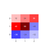
(a)

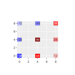
(b)

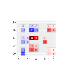
(c)

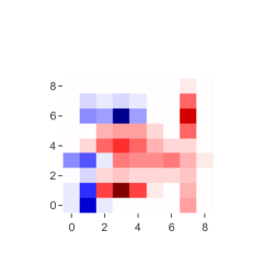
(d)

Figure 1: (a) a standard $3\times 3$ kernel. (b) a standard dilated $3\times 3$ kernel. (c) a 2D-DCLS kernel using bilinear interpolation with 9 kernel elements and a kernel size of 9. (d) the same kernel as (c) with Gaussian interpolation. The numbers have been rounded in all figures and omitted in (d) for readability.

The main focus of this paper will be to question the choice of bilinear interpolation used by default in DCLS. We tested several interpolations and found in particular that a Gaussian interpolation with learnable standard deviations made the approach more effective.

To evaluate the effectiveness of DCLS with Gaussian interpolation, we integrate it as a drop-in replacement for the standard depthwise separable convolution in two state-of-the-art convolutional models: the ConvNext-T model Liu et al. (2022) and the ConvFormer-S18 model Yu et al. (2022). In Section 5, we evaluate the training loss and the classification accuracy of these models on the ImageNet1k dataset Deng et al. (2009). The remainder of this paper will present a detailed analysis of the methods, equations, algorithms and techniques regarding the application of the Gaussian interpolation in DCLS.

2 Related work

In the field of convolutional neural networks (CNNs), various approaches have been explored to improve the performance and efficiency of convolutional operations. Gaussian mixture convolutional networks have investigated the fit of input channels with Gaussian mixtures Celarek et al. (2022), while Chen et al. (2023) utilized Gaussian masks in their work. Additionally, continuous kernel convolution was studied in the context of image processing by Kim & Park (2023). Their approach is similar to the linear correlation introduced in Thomas et al. (2019). The interpolation function used in the last two works corresponds to the DCLS-Triangle method described in 3.1. Romero et al. have also made notable contributions in learning continuous functions that map the positions to the weights Romero et al. (2022a; b).

In the work by Jacobsen et al. (2016), the kernel is represented as a weighted sum of basis functions, including centered Gaussian filters and their derivatives. Pintea et al. (2021) extended this approach by incorporating the learning of Gaussian width, effectively optimizing the resolution. Shelhamer et al. (2019) introduced a kernel factorization method where the kernel is expressed as a composition of a standard kernel and a structured Gaussian one. In these last three works the Gaussians are centered on the kernel.

Furthermore, the utilization of bilinear interpolation within deformable convolution modules has already shown its effectiveness. Dai et al. (2017), Qi et al. (2017) and recently Wang et al. (2022) leveraged bilinear interpolation to smoothen the non-differentiable regular-grid offsets in the deformable convolution method. Even more recently, in Kim et al. (2023), a Gaussian attention bias with learnable standard deviations has been successfully used in the positional embedding of the attention module of the ViT model Dosovitskiy et al. (2021) and leads to reasonable gains on ImageNet1k.

3 Methods

3.1 From bilinear to Gaussian interpolation

We denote by $m\in\mathbb{N}^{*}$ the number of kernel elements inside the dilated constructed kernel and we refer to it as the “kernel count”. Moreover, we denote respectively by $s_{x},s_{y}\in\mathbb{N}^{*}\times\mathbb{N}^{*}$, the sizes of the constructed kernel along the x-axis and the y-axis. The latter could be seen as the limits of the dilated kernel, and we refer to them as the “dilated kernel size”.

The $s_{x}\times s_{y}$ matrix space over $\mathbb{R}$ is defined as the set of all $s_{x}\times s_{y}$ matrices over $\mathbb{R}$, and is denoted $\mathcal{M}_{s_{x},s_{y}}(\mathbb{R})$. The real numbers $w$, $p^{x}$, $\sigma^{x}$, $p^{y}$ and $\sigma^{y}$ respectively stand for the weight, the mean position and standard deviation of that weight along the x-axis (width) and its mean position and standard deviation along the y-axis (height).

The mathematical construction of the 2D-DCLS kernel in Khalfaoui-Hassani et al. (2023) relies on bilinear interpolation and is described as follows :

$$\begin{split}f\colon\mathbb{R}\times\mathbb{R}\times\mathbb{R}&\to\mathcal{M}_{s_{x},s_{y}}(\mathbb{R})\\ w,p^{x},p^{y}&\mapsto\quad K\end{split}$$ (1)

where $\forall i\in\llbracket 1\ ..\ s_{x}\rrbracket$, $\forall j\in\llbracket 1\ ..\ s_{y}\rrbracket\colon$

$$K_{ij}=\left\{\begin{array}[]{cl}w\ (1-r^{x})\ (1-r^{y})&\text{if }i=\lfloor p^{x}\rfloor,\ j=\lfloor p^{y}\rfloor\\ w\ r^{x}\ (1-r^{y})&\text{if }i=\lfloor p^{x}\rfloor+1,\ j=\lfloor p^{y}\rfloor\\ w\ (1-r^{x})\ r^{y}&\text{if }i=\lfloor p^{x}\rfloor,\ j=\lfloor p^{y}\rfloor+1\\ w\ r^{x}\ r^{y}&\text{if }i=\lfloor p^{x}\rfloor{+}1,\ j=\lfloor p^{y}\rfloor{+}1\\ 0&\text{otherwise }\end{array}\right.$$ (2)

and where the fractional parts are:

$$\begin{array}[]{ccc}r^{x}=\{p^{x}\}=p^{x}-\lfloor p^{x}\rfloor&\text{and}&r^{y}=\{p^{y}\}=p^{y}-\lfloor p^{y}\rfloor\end{array}$$ (3)

An equivalent way of describing the constructed kernel $K$ in Equation 2 is:

$$K_{ij}=w\cdot g(p^{x}-i)\cdot g(p^{y}-j)$$ (4)

with

$$g\colon x\mapsto\text{max}(0,\ 1-|x|)$$ (5)

This expression corresponds to the bilinear interpolation as described in Dai et al. (2017, eq. 4).

In fact, this last $g$ function is known as the triangle function (refer to Fig. 2 for a graphic representation), and is widely used in kernel density estimation. From now on, we will note it as

$$\forall x\in\mathbb{R}\quad\quad\Lambda(x)\overset{\text{def}}{=}\text{max}(0,\ 1-|x|)$$ (6)

First, we consider a scaling by a parameter $\sigma\in\mathbb{R}_{+}$ for the triangle function (the bilinear interpolation corresponds to $\sigma=1$),

$$\forall x\in\mathbb{R},\quad\forall\sigma\in\mathbb{R}_{+}\quad\Lambda_{\sigma}(x)\overset{\text{def}}{=}\text{max}(0,\ \sigma-|x|)$$ (7)

We found that this scaling parameter $\sigma$ could be learned by backpropagation and that doing so increases the performance of the DCLS method. As we have different $\sigma$ parameters for the x and y-axes in 2D-DCLS, learning the standard deviations costs two additional learnable parameters and two additional FLOPs (multiplied by the number of the channels of the kernel and the kernel count). We refer to the DCLS method with triangle function interpolation as the DCLS-Triangle method.

Second, we tried a smoother function rather than the piecewise affine triangle function, namely the Gaussian function:

$$\begin{array}[]{lcrr}\forall x\in\mathbb{R},\ \forall\sigma\in\mathbb{R}^{*},&G_{\sigma}(x)\overset{\text{def}}{=}\text{exp}\left({-{\dfrac{x^{2}}{2\sigma^{2}}}}\right)&&\end{array}$$ (8)

We refer to the DCLS method with Gaussian interpolation as the DCLS-Gauss method. In practice, instead of Equations 7 and 8, we respectively use:

$$\forall x\in\mathbb{R},\ \forall\sigma\in\mathbb{R},\enskip\Lambda_{\sigma_{0}+\sigma}(x)=\text{max}(0,\ \sigma_{0}+|\sigma|-|x|)$$ (9)

$$\forall x\in\mathbb{R},\ \forall\sigma\in\mathbb{R},\enskip G_{\sigma_{0}+\sigma}(x)=\text{exp}\left({-\dfrac{1}{2}\dfrac{x^{2}}{(\sigma_{0}+|\sigma|)^{2}}}\right)$$ (10)

with $\sigma_{0}\in\mathbb{R}^{*}_{+}$ a constant that determines the minimum standard deviation that the interpolation could reach. For the triangle interpolation, we take $\sigma_{0}=1$ in order to have at least 4 adjacent interpolation values (see Figure 1c). And for the Gaussian interpolation, we set $\sigma_{0}=0.27$.

Last, to make the sum of the interpolation over the dilated kernel size equal to 1, we divide the interpolations by the following normalization term :

$$A=\epsilon+\sum_{i=1}^{s_{x}}\sum_{j=1}^{s_{y}}\mathcal{I}_{\sigma_{0}+\sigma^{x}}(p^{x}-i)\cdot\mathcal{I}_{\sigma_{0}+\sigma^{y}}(p^{y}-j)$$ (11)

with $\mathcal{I}$ an interpolation function ($\Lambda$ or $G$ in our case) and $\epsilon=1e-7$ for example, to avoid division by zero.

Other interpolations Based on our tests, other functions such as Lorentz, hyper-Gaussians and sinc functions have been tested with no great success. In addition, learning a correlation parameter $\rho\in[-1,1]$ or equivalently a rotation parameter $\theta\in[0,2\pi]$ as in the bivariate normal distribution density did not improve performance (maybe because cardinal orientations predominate in natural images).

3.2 The 2D-DCLS-Gauss kernel construction algorithm

In the following, we describe with pseudocode the kernel construction used in 2D-DCLS-Gauss and 2D-DCLS-Triangle. $\mathcal{I}$ is the interpolation function ($\Lambda$ or $G$ in our case) and $\epsilon=1e-7$. In practice, $w$, $p^{x}$, $p^{y}$, $\sigma^{x}$ and $\sigma^{y}$ are 3-D tensors of size (channels_out, channels_in // groups, K_count), but the algorithm presented here is easily extended to this case by applying it channel-wise.

0:  $w$, $p^{x}$, $p^{y}$, $\sigma^{x}$, $\sigma^{y}$ : vectors of dimension $m$

0:  $K$ : the constructed kernel, of size ($s_{x}\times s_{y}$)

1:  $K\leftarrow 0_{s_{x},s_{y}}$ {zero tensor of size $s_{x},s_{y}$}

2:  for $k=0$ to $m-1$ do

3:     $H\leftarrow 0_{s_{x},s_{y}}$

4:     $p_{k}^{x}\leftarrow p_{k}^{x}+s_{x}//2$; $\quad p_{k}^{y}\leftarrow p_{k}^{y}+s_{y}//2$

5:     $\sigma_{k}^{x}\leftarrow|\sigma_{k}^{x}|+\sigma_{0}^{\mathcal{I}}$; $\quad\sigma_{k}^{y}\leftarrow|\sigma_{k}^{y}|+\sigma_{0}^{\mathcal{I}}$

6:     for $i=0$ to $s^{x}-1$ do

7:        for $j=0$ to $s^{y}-1$ do

8:           $H[i,j]\leftarrow\mathcal{I}_{\sigma_{k}^{x}}(p_{k}^{x}-i)*\mathcal{I}_{\sigma_{k}^{y}}(p_{k}^{y}-j)$

9:        end for

10:     end for

11:     $H[:,:]\leftarrow H[:,:]\ /(\epsilon+\sum\limits_{i=0}^{s^{x}-1}\sum\limits_{j=0}^{s^{y}-1}H[i,j])$

12:     $K\leftarrow K+H*w_{k}$

13:  end for

Algorithm 1 2D-DCLS-interpolation kernel construction

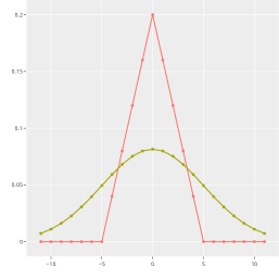
Figure 2: 1D view of Gaussian and $\Lambda$ functions with $\sigma=5$.

Table 1: Classification accuracy on the validation set and training loss on ImageNet-1K. For the 17/34 bilinear, the 23/26 Triangle and Gaussian cases, the results have been averaged over 3 distinct seeds (the corresponding lines are highlighted in yellow).

$$\begin{array}[]{lcccccc}\hline\cr\hline\cr\text{ model @ 224}&\begin{array}[]{l}\text{ ker. size }\\ \text{ / count }\end{array}&\text{interpolation}&\text{ \# param.}&\text{ train loss }&\text{ Top-5 acc.}&\text{ Top-1 acc.}\\ \hline\cr\rule[0.0pt]{0.0pt}{14.45377pt}\ignorespaces\text{ ConvNeXt-T }\squareneswfill&7^{2}\ /\ 49&&28.59\mathrm{M}&2.828&96.05&82.08\\ \text{ ConvNeXt-T }\squarecrossfill&17^{2}\ /\ 34&\text{Bilinear}&28.59\mathrm{M}&2,775&96.11&82.44\\ \text{ ConvNeXt-T }\odot&23^{2}\ /\ 26&\text{Triangle}&28.59\mathrm{M}&2.787&96.09&82.34\\ \text{ ConvNeXt-T }\star&23^{2}\ /\ 26&\text{Gaussian}&28.59\mathrm{M}&2.762&96.18&82.44\\ \text{ ConvNeXt-T }&17^{2}\ /\ 26&\text{Gaussian}&28.59\mathrm{M}&2.773&96.17&82.40\\ \text{ ConvNeXt-T }&23^{2}\ /\ 34&\text{Gaussian}&28.69\mathrm{M}&2.758&96.22&82.60\\ \hline\cr\text{ ConvFormer-S18 }\squareneswfill&7^{2}\ /\ 49&&26.77\mathrm{M}&2.807&96.17&82.84\\ \text{ ConvFormer-S18 }\squarecrossfill&17^{2}\ /\ 40&\text{Bilinear}&26.76\mathrm{M}&2.764&96.42&83.14\\ \text{ ConvFormer-S18 }\odot&23^{2}\ /\ 26&\text{Triangle}&26.76\mathrm{M}&2.761&96.38&83.09\\ \text{ ConvFormer-S18 }\star&23^{2}\ /\ 26&\text{Gaussian}&26.76\mathrm{M}&2.747&96.31&82.99\\ \hline\cr\hline\cr\end{array}$$

4 Learning techniques

Having discussed the implementation of the interpolation in the DCLS method, we now shift our focus to the techniques employed to maximize its potential. We retained most of the techniques used in Khalfaoui-Hassani et al. (2023), and suggest new ones for learning standard deviations parameters. In Appendix C, we present the training techniques that have been selected based on consistent empirical evidence, yielding improved training loss and validation accuracy.

5 Results

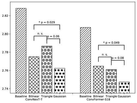
Figure 3: Training loss for ConvNeXt-T and ConvFormer-S18 models with DCLS according to interpolation type (lower is better). The pairwise p-values have been calculated using an independent two-sample Student t-test assuming equal variances. The vertical line segments stand for the standard errors.

We took two recent state-of-the-art convolutional architectures, ConvNeXt and ConvFormer, and drop-in replaced all the depthwise convolutions by DCLS ones, using the three different interpolations (bilinear, triangle or Gauss). Table 1 reports the results in terms of training loss and validation accuracy.

A first observation is that all the DCLS models perform much better than the baselines, whereas they have the same number of parameters. There are also subtle differences between interpolation functions. As Figure 3 shows, triangle and bilinear interpolations perform similarly, but the Gaussian interpolation performs significantly better.

Furthermore, the advantage of the Gaussian interpolation w.r.t. bilinear is not only due to the use of a larger kernel, as a 17x17 Gaussian kernel (5th line in Table 1) still outperforms the bilinear case (2nd line). Finally, the 6th line in Table 1 shows that there is still room for improvement by increasing the kernel count, although this slightly increases the number of trainable parameters w.r.t. the baseline.

6 Conclusion

In conclusion, this study introduces Gaussian and $\Lambda$ interpolation methods as alternatives to bilinear interpolation in Dilated Convolution with Learnable Spacings (DCLS). Evaluations on state-of-the-art convolutional architectures demonstrate that Gaussian interpolation improves performance of image classification task on ImageNet1k without increasing parameters. Future work could implement the Whittaker-Shannon interpolation instead of the Gaussian interpolation and search for a dedicated architecture, that will make the most of DCLS.

Appendix A Code and reproducibility

The code of the method is based on PyTorch and available at https://github.com/K-H-Ismail/Dilated-Convolution-with-Learnable-Spacings-PyTorch.

Appendix B Pytorch implementation of the 2D-DCLS-Gauss and 2D-DCLS-Triangle forward algorithm

⬇

1class ConstructKernel2d(Module):

2 def __init__(self, out_channels, in_channels, groups, kernel_count, dilated_kernel_size, version):

3 super().__init__()

4 self.version = version

5 self.out_channels, self.in_channels = out_channels, in_channels

6 self.groups = groups

7 self.dilated_kernel_size = dilated_kernel_size

8 self.kernel_count = kernel_count

9 self.IDX, self.lim = None, None

10

11 def __init_tmp_variables__(self, device):

12 if self.IDX is None or self.lim is None:

13 J = Parameter(torch.arange(0, self.dilated_kernel_size[0]),

14 requires_grad=False).to(device)

15 I = Parameter(torch.arange(0, self.dilated_kernel_size[1]),

16 requires_grad=False).to(device)

17 I = I.expand(self.dilated_kernel_size[0],-1)

18 J = J.expand(self.dilated_kernel_size[1],-1).t()

19 IDX = torch.cat((I.unsqueeze(0),J.unsqueeze(0)), 0)

20 IDX = IDX.expand(self.out_channels, self.in_channels//self.groups,

21 self.kernel_count,-1,-1,-1).permute(4,5,3,0,1,2)

22 self.IDX = IDX

23 lim = torch.tensor(self.dilated_kernel_size).to(device)

24 self.lim = lim.expand(self.out_channels,

25 self.in_channels//self.groups, self.kernel_count, -1).permute(3,0,1,2)

26 else:

27 pass

28

29 def forward_vtriangle(self, W, P, SIG):

30 P = P + self.lim // 2

31 SIG = SIG.abs() + 1.0

32 X = (self.IDX - P)

33 X = ((SIG - X.abs()).relu()).prod(2)

34 X = X / (X.sum((0,1)) + 1e-7) # normalization

35 K = (X * W).sum(-1)

36 K = K.permute(2,3,0,1)

37 return K

38

39 def forward_vgauss(self, W, P, SIG):

40 P = P + self.lim // 2

41 SIG = SIG.abs() + 0.27

42 X = ((self.IDX - P) / SIG).norm(2, dim=2)

43 X = (-0.5 * X**2).exp()

44 X = X / (X.sum((0,1)) + 1e-7) # normalization

45 K = (X * W).sum(-1)

46 K = K.permute(2,3,0,1)

47 return K

48

49 def forward(self, W, P, SIG):

50 self.__init_tmp_variables__(W.device)

51 if self.version == ’triangle’:

52 return self.forward_vtriangle(W, P, SIG)

53 elif self.version == ’gauss’:

54 return self.forward_vgauss(W, P, SIG)

55 else:

56 raise

Appendix C Learning techniques

• Weight decay: No weight decay was used for positions. We apply the same for standard deviation parameters.

• Positions and standard deviations initialization: position parameters were initialized following a centered normal law of standard deviation 0.5. Standard deviation parameters were initialized to a constant $0.23$ in DCLS-Gauss and to $0$ in DCLS-Triangle in order to have a similar initialisation to DCLS with bilinear interpolation at the beginning.

• Positions clamping : Previously in DCLS, kernel elements that reach the dilated kernel size limit were clamped. It turns out that this operation is no longer necessary with the Gauss and $\Lambda$ interpolations.

• Dilated kernel size tuning: When utilizing bilinear interpolation in ConvNeXt-dcls, a dilated kernel size of 17 was found to be optimal, as larger sizes did not yield improved accuracy. However, with Gaussian and $\Lambda$ interpolations, there appears to be no strict limit to the dilated kernel size. Accuracy tends to increase logarithmically as the size grows, with improvements observed up to kernel sizes of 51. It is important to note that increasing the dilated kernel size does not impact the number of trainable parameters, but it does affect throughput. Therefore, a compromise between accuracy and throughput was achieved by setting the dilated kernel size to 23.

• Kernel count tuning: This hyper-parameter has been configured to the maximum integer value while still remaining below the baselines to which we compare ourselves in terms of trainable parameters. It is worth noting that each additional element in the 2D-DCLS-Gauss or 2D-DCLS-Triangle methods introduces five more learnable parameters: weight, vertical and horizontal position, and their respective standard deviations. To maintain simplicity, the same kernel count was applied across all model layers.

• Learning rate scaling: To maintain consistency between positions and standard deviations, we applied the same learning rate scaling ratio of 5 to both. In contrast, the learning rate for weights remained unchanged.

• Synchronizing positions: we shared the kernel positions and standard deviations across convolution layers with the same number of parameters, without sharing the weights. Parameters in these stages were centralized in common parameters that accumulate the gradients.

Appendix D 1D and 3D convolution cases

For the 3D case, Equation 4 can be generalized as a product along spatial dimensions. We denote respectively by $s_{x},s_{y},s_{z}\in\mathbb{N}^{*}\times\mathbb{N}^{*}\times\mathbb{N}^{*}$, the sizes of the constructed kernel along the x-axis, the y-axis and the z-axis. The constructed kernel tensor $K^{3D}\in\mathcal{M}_{s_{x},s_{y},s_{z}}(\mathbb{R})$ is therefore:

$\forall i\in\llbracket 1\ ..\ s_{x}\rrbracket$, $\forall j\in\llbracket 1\ ..\ s_{y}\rrbracket$, $\forall k\in\llbracket 1\ ..\ s_{z}\rrbracket\colon$

$$K^{3D}_{ijk}=w\cdot\mathcal{I}_{\sigma_{0}+\sigma^{x}}(p^{x}-i)\cdot\mathcal{I}_{\sigma_{0}+\sigma^{y}}(p^{y}-j)\cdot\mathcal{I}_{\sigma_{0}+\sigma^{z}}(p^{z}-k)$$ (12)

with $\mathcal{I}$ an interpolation function ($\Lambda$ or $G$), $\sigma_{0}=1$ for the $\Lambda$ interpolation and $\sigma_{0}=0.27$ for the Gaussian one. $w$, $p^{x}$, $\sigma^{x}$, $p^{y}$, $\sigma^{y}$, $p^{z}$ and $\sigma^{z}$ respectively representing the weight, the mean position and standard deviation of that weight along the x-axis (width), the mean position and standard deviation along the y-axis (height) and its mean position and standard deviation along the z-axis (depth).

The constructed kernel vector $K^{1D}\in\mathbb{R}^{s_{x}}$ for the 1D case is simply:

$\forall i\in\llbracket 1\ ..\ s_{x}\rrbracket\colon$

$$K^{1D}_{i}=w\cdot\mathcal{I}_{\sigma_{0}+\sigma^{x}}(p^{x}-i)$$ (13)

The Algorithm 1 as well as the Pytorch code B are readily adapted to these cases by following the above note.

References

- Celarek et al. (2022) Celarek, A., Hermosilla, P., Kerbl, B., Ropinski, T., and Wimmer, M. Gaussian mixture convolution networks. In International Conference on Learning Representations, 2022.
- Chen et al. (2023) Chen, Q., Li, C., Ning, J., and He, K. Gaussian mask convolution for convolutional neural networks. arXiv preprint arXiv:2302.04544, 2023.
- Dai et al. (2017) Dai, J., Qi, H., Xiong, Y., Li, Y., Zhang, G., Hu, H., and Wei, Y. Deformable convolutional networks. In Int. Conf. Comput. Vis., pp. 764–773, 2017.
- Deng et al. (2009) Deng, J., Dong, W., Socher, R., Li, L.-J., Li, K., and Fei-Fei, L. Imagenet: A large-scale hierarchical image database. In Proc. IEEE/CVF Conf. Comput. Vis. Pattern Recog. (CVPR), pp. 248–255. IEEE, 2009.
- Ding et al. (2022) Ding, X., Zhang, X., Han, J., and Ding, G. Scaling up your kernels to 31x31: Revisiting large kernel design in CNNs. In Proc. IEEE/CVF Conf. Comput. Vis. Pattern Recog. (CVPR), pp. 11963–11975, 2022.
- Dosovitskiy et al. (2021) Dosovitskiy, A., Beyer, L., Kolesnikov, A., Weissenborn, D., Zhai, X., Unterthiner, T., Dehghani, M., Minderer, M., Heigold, G., Gelly, S., et al. An image is worth 16x16 words: Transformers for image recognition at scale. In International Conference on Learning Representations, 2021.
- Jacobsen et al. (2016) Jacobsen, J.-H., Van Gemert, J., Lou, Z., and Smeulders, A. W. Structured receptive fields in cnns. In Proceedings of the IEEE Conference on Computer Vision and Pattern Recognition, pp. 2610–2619, 2016.
- Khalfaoui-Hassani et al. (2023) Khalfaoui-Hassani, I., Pellegrini, T., and Masquelier, T. Dilated convolution with learnable spacings. In The Eleventh International Conference on Learning Representations, 2023. URL https://openreview.net/forum?id=Q3-1vRh3HOA.
- Kim et al. (2023) Kim, B. J., Choi, H., Jang, H., and Kim, S. W. Understanding gaussian attention bias of vision transformers using effective receptive fields. arXiv preprint arXiv:2305.04722, 2023.
- Kim & Park (2023) Kim, S. and Park, E. Smpconv: Self-moving point representations for continuous convolution. arXiv preprint arXiv:2304.02330, 2023.
- Liu et al. (2022) Liu, Z., Mao, H., Wu, C.-Y., Feichtenhofer, C., Darrell, T., and Xie, S. A convnet for the 2020s. In Proc. IEEE/CVF Conf. Comput. Vis. Pattern Recog. (CVPR), pp. 11976–11986, 2022.
- Pintea et al. (2021) Pintea, S. L., Tömen, N., Goes, S. F., Loog, M., and van Gemert, J. C. Resolution learning in deep convolutional networks using scale-space theory. IEEE Transactions on Image Processing, 30:8342–8353, 2021.
- Qi et al. (2017) Qi, H., Zhang, Z., Xiao, B., Hu, H., Cheng, B., Wei, Y., and Dai, J. Deformable convolutional networks–coco detection and segmentation challenge 2017 entry. In Proc. ICCV COCO Challenge Workshop, volume 15, pp. 1, 2017.
- Romero et al. (2022a) Romero, D. W., Bruintjes, R., Bekkers, E. J., Tomczak, J. M., Hoogendoorn, M., and van Gemert, J. Flexconv: Continuous kernel convolutions with differentiable kernel sizes. In 10th International Conference on Learning Representations, 2022a.
- Romero et al. (2022b) Romero, D. W., Kuzina, A., Bekkers, E. J., Tomczak, J. M., and Hoogendoorn, M. CKConv: Continuous kernel convolution for sequential data. In International Conference on Learning Representations, 2022b. URL https://openreview.net/forum?id=8FhxBtXSl0.
- Shelhamer et al. (2019) Shelhamer, E., Wang, D., and Darrell, T. Blurring the line between structure and learning to optimize and adapt receptive fields. arXiv preprint arXiv:1904.11487, 2019.
- Thomas et al. (2019) Thomas, H., Qi, C. R., Deschaud, J.-E., Marcotegui, B., Goulette, F., and Guibas, L. J. Kpconv: Flexible and deformable convolution for point clouds. Int. Conf. Comput. Vis., 2019.
- Wang et al. (2022) Wang, W., Dai, J., Chen, Z., Huang, Z., Li, Z., Zhu, X., Hu, X., Lu, T., Lu, L., Li, H., et al. Internimage: Exploring large-scale vision foundation models with deformable convolutions. arXiv preprint arXiv:2211.05778, 2022.
- Yu et al. (2022) Yu, W., Si, C., Zhou, P., Luo, M., Zhou, Y., Feng, J., Yan, S., and Wang, X. Metaformer baselines for vision. arXiv preprint arXiv:2210.13452, 2022.