Fermonic anyons: entanglement and quantum computation from a resource-theoretic perspective

Abstract

Often quantum computational models can be understood via the lens of resource theories, where a computational advantage is achieved by consuming specific forms of quantum resources and, conversely, resource-free computations are classically simulable. For example, circuits of nearest-neighbor matchgates can be mapped to free-fermion dynamics, which can be simulated classically. Supplementing these circuits with nonmatchgate operations or non-gaussian fermionic states, respectively, makes them quantum universal. Can we similarly identify quantum computational resources in the setting of more general quasi-particle statistics, such as that of fermionic anyons? In this work, we develop a resource-theoretic framework to define and investigate the separability of fermionic anyons. We build the notion of separability through a fractional Jordan-Wigner transformation, leading to a Schmidt decomposition for fermionic-anyon states. We show that this notion of fermionic-anyon separability, and the unitary operations that preserve it, can be mapped to the free resources of matchgate circuits. We also identify how entanglement between two qubits encoded in a dual-rail manner, as standard for matchgate circuits, corresponds to the notion of entanglement between fermionic anyons. Though this does not coincide with the usual definition of qubit entanglement, it provides new insight into the limited capabilities of matchgate circuits.

Introduction. Over the last five decades, our notion of identical particles in nature has expanded beyond fermions and bosons. Many two-dimensional systems were shown to contain anyonic excitations Wilczek (1982); Nayak et al. (2008), which are quasi-particles characterised by the non-trivial phases their wave functions acquire under particle exchange. These include fractional quantum Hall states Arovas et al. (1984); Stern (2008), topological spin liquids Savary and Balents (2016); Zhou et al. (2017), and semiconductor nanowire arrays Stanescu and Tewari (2013); Sarma et al. (2015). These systems are seen as possible platforms for fault-tolerant quantum computing Wilczek (1982); Sarma et al. (2015), given their inherent error-correcting properties Fowler et al. (2012); Brell (2015); Litinski and Oppen (2018) and the recent experimental evidence of their existence and predicted properties Nakamura et al. (2020).

Although anyons are most commonly associated with two-dimensional systems, they can also be defined in one dimension. Some notable examples are anyons obtained by dimensional reduction Hansson et al. (1991); Ha (1995), and anyons appearing as a free-particle description of one-dimensional systems with two-body interactions Lieb and Liniger (1963); Calogero (1969); Haldane (1988); Shastry (1988); Olshanetsky and Perelomov (1983). The one dimensional anyons considered in this letter are motivated by their role in solving many-body systems with three-body interactions Kundu (1999); Batchelor et al. (2006); Batchelor and Guan (2006); Calabrese and Caux (2007); Pâţu et al. (2007); Hao et al. (2008); Keilmann et al. (2011) and have been subject to investigations in optical lattice implementations Greschner et al. (2014); Cardarelli et al. (2016); Liang et al. (2018); Schweizer et al. (2019). Although they lack the topological properties of their two-dimensional counterparts Harshman and Knapp (2020), their relation to standard fermionic and bosonic systems via generalised Jordan-Wigner transformations Meljanac et al. (1994); Dorešić et al. (1994); Meljanac and Mileković (1996) makes them a good case study for generalisations of quantum computing with bosonic and fermionic linear optics.

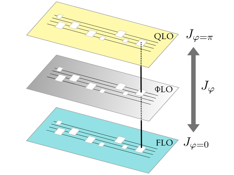
Figure 1: Representation of universal quantum computation for different algebras. It is a pictorial representation of a fermionic anyon quantum circuit mapping different algebraic representations, from $\varphi=[0,\pi]$, by the fractional Jordan-Wigner transformation $J_{\varphi}$. The extremal cases of $\varphi=0$ and $\varphi=\pi$ translate fermionic linear optics operations, and qubit linear optics operations (matchgates quantum computation with dual rail encoding), respectively. The dotted-line connecting the quantum gate represents that each quantum gate has an isomorphic counterpart in each algebraic representation, connected by $J_{\varphi}$.

In this letter, we develop a resource-theoretic framework to define and investigate the separability of fermionic anyons. Since this is well-understood for fermions, the naive approach is to directly repurpose definitions and measures of fermionic entanglement to their anyonic counterparts Bonderson et al. (2017); Mani et al. (2020); Zhang et al. (2020); Sreedhar and Ramadas (2022). However, this sometimes leads to nonsensical results. For example, performing a standard particle partial trace to obtain the state of a subsystem of fermionic anyons leads to density matrices that depend on unphysical particle labels (i.e., not invariant under particle permutations). Similarly, single-particle transformations on a manifestly unentangled state can result in states with Schmidt rank greater than one—thus with a nonzero entanglement entropy. Within a subspace of fixed particle number, we circumvent these problems by proposing a novel and well-motivated definition of the Schmidt coefficients of a composite fermionic-anyon state based on a non-canonical transformation over the anyonic state. Specifically, we map the anyonic algebra to another system that satisfies an anti-commutative algebra. We prove that the Schmidt coefficients of the original anyonic state are the same as the mapped state.

As a way to corroborate our definition, we further investigate the connection between notions of separability and classical simulability in these systems. Care must be taken when trying to make this connection: there are highly-entangled systems that are classically simulable Aaronson and Gottesman (2004); Gottesman (1998), universal quantum computers that work with vanishingly small entanglement Van den Nest (2013), as well as systems of free bosons capable of demonstrating quantum computational advantage Aaronson and Arkhipov (2011). Nevertheless, there is one setting where separability and computational power are more tightly connected, that of free-fermionic Terhal and DiVincenzo (2002) or matchgate computing Valiant (2002); Jozsa and Miyake (2008). Nearest-neighbor matchgate circuits correspond (via a Jordan-Wigner transformation) to free-fermion dynamics, and both are known to be classically simulable. However, it can be shown that supplementing these systems with any non-matchgate operation (in the fermionic picture, adding an interaction between particles) or any non-matchgate generated state (respectively, any non-Gaussian fermionic state) is enough to allow for universal quantum computation. Here, we leverage this connection to make a similar statement for fermionic anyons. In particular, we show that both nonseparable states or transformations, as per our definition, can be seen as computational resources. Moreover, we can interpret limiting values of the fermionic-anyon phase $\varphi$ to recover well-known results. Fermionic-anyon dynamics reduces to fermionic linear optics when $\varphi=0$, and to “qubit linear optics” (or matchgate quantum computing) when $\varphi=\pi$, if we interpret each physical qubit as the occupation number of a fermionic-anyon mode, as illustrated in Fig. 1.

Fermionic anyons. Given a one-dimensional (1D) set of $m$ sites (or modes), we define a family of operator algebras $\{\mathcal{A}^{\varphi}_{m}|\text{ }\varphi\in[0,2\pi)\}$, where each $\mathcal{A}^{\varphi}_{m}$ is an operator algebra over $\mathbb{C}$ generated by operators $\{a_{\varphi,i}|\text{ }i=1,...,m\}$ satisfying

$$\begin{split}&a_{\varphi,i}a_{\varphi,j}^{\dagger}+e^{-i\varphi\epsilon_{ij}}a_{\varphi,j}^{\dagger}a_{\varphi,i}=\delta_{ij},\\ &a_{\varphi,i}a_{\varphi,j}+e^{i\varphi\epsilon_{ij}}a_{\varphi,j}a_{\varphi,i}=0,\end{split}$$ (1)

with $\epsilon_{ij}$ given by

$$\epsilon_{ij}=\left\{\begin{matrix}1,&\textnormal{if}\ \ i<j\\ 0,&\textnormal{if}\ \ i=j\\ -1,&\textnormal{if}\ \ i>j.\end{matrix}\right.$$

The variable $\varphi$ is called the statistical parameter, and it determines the kind of particle described by the algebra. If $\varphi=0$, the operators satisfy canonical anticommutation relations, and we identify $f_{i}:=a_{0,i}$, and $\mathcal{F}_{m}\equiv\mathcal{A}^{0}_{m}$ where $\mathcal{F}_{m}$ is the algebra of $m$-mode fermionic operators. Similarly, if $\varphi=\pi$ then for all $i,j$ we have $[a_{\pi,i},a_{\pi,j}]=0$ as well as $\{a_{\pi,i},a^{\dagger}_{\pi,j}\}=0$, and we identify $\mathcal{A}^{\pi}_{m}\equiv\mathcal{Q}_{m}$, where $\mathcal{Q}_{m}$ is the algebra of operators for $m$-mode hardcore bosons, or qubits Wu and Lidar (2002). For any other value of $\varphi$, the algebra $\mathcal{A}^{\varphi}_{m}$ describes particles with exotic exchange statistics called fermionic anyons.

In the Supplemental Material SM we prove that, for all $\varphi$, the algebras $\mathcal{A}^{\varphi}_{m}$ have a well-defined Fock-space representation, denoted by $\mathbb{A}^{\varphi}_{m}$, with number operators of the form $a^{\dagger}_{\varphi,i}a_{\varphi,i}$. Therefore, a general pure state of $N$ fermionic anyons has the form

$$\ket{\psi}=\sum_{I_{N}}w_{I_{N}}a_{\varphi,i_{1}}^{\dagger}...a_{\varphi,i_{N}}^{\dagger}\ket{\textrm{vac}},$$ (2)

where $\ket{\textrm{vac}}$ is the vacuum state, $I_{N}=\{i_{1}<...<i_{N}\}$ is a shorthand for the list of particle indices, and $\sum_{I_{N}}|w_{I_{N}}|^{2}=1$.

Separability for fermionic anyons. For a quantum system with two sets of degrees of freedom, a standard quantifier of correlations for pure states is the entanglement entropy Nielsen and Chuang (2010),

$$E(\ket{\psi})=\log{m}-S(\rho_{\textrm{red}}).$$ (3)

Here, $S(\rho)$ is the von Neumann entropy of $\rho$, and $\rho_{\textrm{red}}$ is the reduced state obtained by tracing out one of the subsystems. However, as highlighted earlier, applying naively a particle partial trace on systems of fermionic anyons can lead to nonsensical results SM . Therefore, we now propose an alternative route to characterise entanglement for fermionic anyons.

First, recall that particle entanglement is a property of a quantum state that is invariant under a particular set of transformations, called single-particle operations. For standard fermions, these operations must act as changes of basis over single-particle systems, implying they have the second-quantized form

$${f}^{\dagger}_{i}\rightarrow Uf_{i}^{\dagger}U^{\dagger}=\sum_{j=1}^{m}U_{ij}f^{\dagger}_{j},$$ (4)

where $U_{ij}$ are elements of an $m\crossproduct m$ unitary matrix. This map is well-defined for fermions because it is canonical, i.e., does not change particle commutation relations. However, defining single-particle operations for fermionic anyons by simple analogy with eq. 4 (i.e. replacing $f$ with $a_{\varphi}$) does not produce a canonical transformation. To properly define these operations for fermionic anyons, we must find an appropriate definition for their canonical transformations.

As shown in Meljanac and Perica (1994); Osterloh et al. (2000), creation and annihilation operators for fermionic anyons (for any $\varphi$) can be identified with operators in the usual fermionic algebra via the relations

$$a_{\varphi,j}=f_{j}e^{-i\varphi\sum^{j-1}_{k=1}f^{\dagger}_{j}f_{j}},\quad a^{\dagger}_{\varphi,j}=f^{\dagger}_{j}e^{i\varphi\sum^{j-1}_{k=1}f^{\dagger}_{j}f_{j}},$$ (5)

known as the fractional Jordan-Wigner transform. It follows that $a^{\dagger}_{\varphi,i}a_{\varphi,i}=f^{\dagger}_{i}f_{i}$, from which we obtain the inverse relationship

$$f_{j}=a_{\varphi,j}e^{i\varphi\sum^{j-1}_{k=1}a^{\dagger}_{\varphi,k}a_{\varphi,k}},\quad f^{\dagger}_{j}=a^{\dagger}_{\varphi,j}e^{-i\varphi\sum^{j-1}_{k=1}a^{\dagger}_{\varphi,k}a_{\varphi,k}}.$$ (6)

These identities imply that any operator in $\mathcal{A}^{\varphi}_{m}$ can be expressed as an operator in $\mathcal{F}_{m}$ and vice-versa, and they are the same operator algebra. In contrast, $\mathcal{A}^{\varphi}_{m}$ and $\mathcal{F}_{m}$ are not isomorphic as Lie-algebras, since they are not related by canonical transformations. Thus, our main proposal is to define the canonical transformations for fermionic anyons as equal to fermionic ones, though written in terms of fermionic-anyon generators via eq. 6. In general, since $\mathcal{A}^{\varphi}_{m}\equiv\mathcal{F}_{m}$ as operator algebras, any operator $O\in\mathcal{F}_{m}$ can be written as

$$[O]_{x}=\sum_{\alpha_{1},...,\alpha_{2m}\in\{0,1\}}c^{x}_{\alpha_{1},...,\alpha_{2m}}x^{\dagger\alpha_{1}}_{1}\cdots{x}^{\dagger\alpha_{m}}_{m}x^{\alpha_{m+1}}_{1}\cdots{x}^{\alpha_{2m}}_{m},$$

where $\{\alpha_{l}\}^{2m}_{l=1}$ are binary variables and, $c^{x}_{\alpha_{1},...,\alpha_{2m}}$ are expansion coefficients. When $x$ stands for $f$ (resp. $a_{\varphi}$), this is called a fermionic (resp. anyonic) form.

We use the fractional Jordan-Wigner transform to define a map $J_{\varphi}$ over operators in $\mathcal{F}_{m}$ that is linear, invertible, preserves operator products and conjugation (see the Supplemental Material SM ), and use it to define the change between the two forms for any operator. In other words, given $O\in\mathcal{F}_{m}$,

$$[O]_{f}=J_{\varphi}([O]_{a_{\varphi}}),\quad[O]_{a_{\varphi}}=J^{-1}_{\varphi}([O]_{f}).$$ (7)

Since an arbitrary fermionic state can be written as

$$\ket{\psi}=\sum_{\alpha_{1},...,\alpha_{m}\in\{0,1\}}\psi^{f}_{\alpha_{1},...,\alpha_{m}}f^{\dagger\alpha_{1}}_{1}\cdots{f}^{\dagger\alpha_{m}}_{m}\ket{0}=:[\psi]_{f}\ket{0},$$

we can use the $J^{-1}_{\varphi}$ to prove (see the Supplemental Material SM ) that

$$\ket{\psi}=[\psi]_{f}\ket{0}=[\psi]_{a_{\varphi}}\ket{0},$$

with $\psi^{f}_{\alpha_{1},...,\alpha_{m}}=\psi^{a_{\varphi}}_{\alpha_{1},...,\alpha_{m}}$ for all pure states $\ket{\psi}$, implying that all Fock states are invariant under the action of $J_{\varphi}$ over operators. Therefore, the fermionic and anyonic forms of any operator $O$ have the same matrix elements over the Fock space, even if the coefficients in the expansions of $[O]_{f}$ and $[O]_{a_{\varphi}}$ are different.

Thus, if $[U]_{f}$ is a single-particle change of basis over fermionic states, then $[U]_{a_{\varphi}}$ must have the same action in terms of fermionic-anyon states. For fermionic systems, an $N$-particle state $\ket{\psi}$ is said to be separable, i.e., it has no particle entanglement Schliemann et al. (2001), if there is an $N$-particle state in the Fock basis and a single-particle operator $U$ such that

$$\ket{\psi}=[U]_{f}(f^{\dagger}_{i_{1}}\cdots f^{\dagger}_{i_{N}})\ket{0},$$ (8)

where we can assume that $i_{1}<...<i_{m}$. These states are described by a single Slater determinant, with only exchange correlations due to its symmetry. We can now extend this notion for general fermionic anyons using the previous transformation, leading to a central definition in this work:

Definition 1 (Separable fermionic anyon states).

A pure $N$-particle fermionic-anyon state $\ket{\phi}$ is separable if and only if there is a single-particle fermionic operator $[U]_{f}$ such that

$$\ket{\phi}=[U]_{a_{\varphi}}(a^{\dagger}_{\varphi,i_{1}}\cdots{a}^{\dagger}_{\varphi,i_{N}})\ket{0}.$$ (9)

Having established separability criteria, we can investigate entanglement in fermionic anyons by adapting corresponding concepts for fermions. Here we focus on the Schmidt decomposition. Using the $J_{\varphi}$ map as translation between fermions and fermionic anyons, it is possible to obtain a dressed Schmidt decomposition for two-particle fermionic-anyon states, as illustrated in fig. 2. This decomposition is obtained by mapping the anyonic state into a fermionic form, calculating the Schliemann coefficients of the fermionic state Schliemann et al. (2001) and translating the new state back into anyonic form. Since $J_{\varphi}$ is a *-algebra endomorphism, we obtain the following theorem (proof is presented in Supplemental Material SM ).

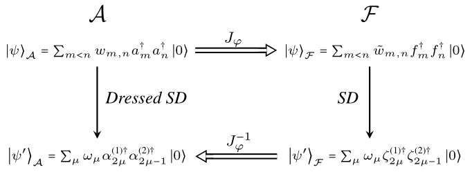
Figure 2: Schmidt decomposition for anyons. Labels $\mathcal{A}$ and $\mathcal{F}$ indicate anyonic and fermionic operator bases, respectively.We first apply the $J_{\varphi}$ map on the anyonic state $\ket{\psi}_{\raisebox{0.0pt}{\tiny{$\mathcal{A}$}}}$, obtaining the fermionic state $\ket{\psi}_{\raisebox{0.0pt}{\tiny{$\mathcal{F}$}}}$. Then, we diagonalize the anti-symmetric matrix $V$, with elements $v_{m,n}=sign(n-m){w}_{m,n}$, to obtain the Schmidt decomposition (SD) Schliemann et al. (2001), represented by the state $\ket{\psi^{\prime}}_{\raisebox{0.0pt}{\tiny{$\mathcal{F}$}}}$. Finally, we apply $J^{-1}_{\varphi}$ on $\ket{\psi^{\prime}}_{\raisebox{0.0pt}{\tiny{$\mathcal{F}$}}}$ to obtain the anyonic state $\ket{\psi^{\prime}}_{\raisebox{0.0pt}{\tiny{$\mathcal{A}$}}}$, where $[\alpha^{(i)}_{2\mu}]_{f}=\zeta^{(i)}_{2\mu}\exp{i\varphi\sum_{k=1}^{2\mu-1}\zeta^{\dagger(i)}_{k}\zeta^{(i)}_{k}}$. The total process performed directly on $\ket{\psi}_{\raisebox{0.0pt}{\tiny{$\mathcal{A}$}}}$ is what we call a dressed Schmidt decomposition (dressed SD).

Theorem 1 (Schmidt decomposition for fermionic anyons).

Any pure state of two fermionic anyons with a fixed number of modes has a Schmidt decomposition with the same expansion coefficients as its Schliemann fermionic state counterpart.

We can expand these considerations to their entanglement properties. Consider a dressed unitary transformation $[U_{SD}]_{a_{\varphi}}$ that maps a fermionic anyon state $\ket{\psi}_{\raisebox{0.0pt}{\tiny{$\mathcal{A}$}}}=\sum_{m<n}w_{m,n}{a}_{m}^{\dagger}a_{n}^{\dagger}\ket{0}$ , written in a given basis, onto its Schmidt decomposition: $\ket{\psi^{\prime}}_{\raisebox{0.0pt}{\tiny{$\mathcal{A}$}}}$ as

$$\ket{\psi^{\prime}}_{\raisebox{0.0pt}{\tiny{$\mathcal{A}$}}}=[U_{SD}]_{a_{\varphi}}\ket{\psi}_{\raisebox{0.0pt}{\tiny{$\mathcal{A}$}}}=\sum_{\mu}{\omega}_{\mu}\alpha^{\text{\tiny{(1)}}\dagger}_{2\mu}\alpha^{\text{\tiny{(2)}}\dagger}_{2\mu-1}\ket{0}.$$ (10)

The dressed transformation $[U_{SD}]_{a_{\varphi}}$ must have the form

$$\ [U_{SD}]_{a_{\varphi}}=J^{-1}_{\varphi}([U_{SD}]_{f}),$$ (11)

where $[U_{SD}]_{f}$ is the single-particle fermionic operator that diagonalises the anti-symmetric matrix $W$ with elements ${\tilde{w}}_{m,n}$ and eigenvalues given by $\omega_{\mu}$. In this way, the entanglement of state $\ket{\psi^{\prime}}_{\raisebox{0.0pt}{\tiny{$\mathcal{A}$}}}$ can be quantified by the entanglement entropy as

$$E(\ket{\psi}_{\raisebox{0.0pt}{\tiny{$\mathcal{A}$}}})=\log(m)+\sum_{\mu=1}^{r}\omega_{\mu}\log(\omega_{\mu}),$$ (12)

where $r$ is the Schmidt rank of the state.

Fermionic linear optics and fermionic anyons. In order to showcase what insights can be drawn from an entanglement theory for fermionic anyons, we apply the formal framework we proposed to particle-based quantum computing.

Let $PS_{i}$, $BS_{i,j}$ and $PA_{i,j}$ be unitary operators of the form

$$PS_{i}(\theta) =\exp[i\theta(a^{\dagger}_{\varphi,i}a_{\varphi,i})]$$ (13)

$$BS_{i,j}(\theta) =\exp[i\theta(a^{\dagger}_{\varphi,i}a_{\varphi,j}+a^{\dagger}_{\varphi,j}a_{\varphi,i})]$$ (14)

$$PA_{i,j}(\theta) =\exp[i\theta(a^{\dagger}_{\varphi,i}a^{\dagger}_{\varphi,j}+a_{\varphi,j}a_{\varphi,i})].$$ (15)

We refer to these unitaries as Gaussian optical elements or, by analogy with linear optics, phase shifters ($PS_{i}$), beam splitters ($BS_{i,j}$), and parametric amplifiers ($PA_{i,j}$).

A product of Gaussian optical elements is called an optical circuit. When $\varphi=0$, this set of transformations acting on Fock states and followed by single-mode number detectors defines a computational model called fermionic linear optics, or FLO. When $\varphi=\pi$, they are called matchgates Jozsa and Miyake (2008), which we refer to here as qubit linear optics or QLO. For any other value of $\varphi$, we refer to quantum computing with optical circuits by fermionic-anyon linear optics, or $\Phi$LO.

Our purpose is to use the $J_{\varphi}$ map to translate known results regarding FLO into results regarding $\Phi$LO and QLO. First, we look at how fermionic optical elements transform under $J^{-1}_{\varphi}$. We are interested in operations that are invariant under $J^{-1}_{\varphi}$, i.e., that have the same operator decomposition in all particle systems. Since phase shifters are generated by Hamiltonians proportional to $f^{\dagger}_{i}f_{i}$, they must be invariant under the action of $J^{-1}_{\varphi}$—as must, in fact, be any operator whose fermionic form contains only products of number operators.

Fermionic beam splitters are generated by Hamiltonians proportional to $f^{\dagger}_{i}f_{j}+f^{\dagger}_{j}f_{i}$. Those are transformed by $J^{-1}_{\varphi}$ into

$$a^{\dagger}_{\varphi,i}e^{i\varphi\sum^{j-1}_{k=i+1}n_{k}}a_{\varphi,j}+a^{\dagger}_{\varphi,j}e^{-i\varphi\sum^{j-1}_{k=i+1}n_{k}}a_{\varphi,i}.$$

This form implies that $J^{-1}_{\varphi}$ leaves only nearest-neighbour beam-splitters invariant. It is known that all single-particle fermionic operators can be decomposed as products of phase shifters and nearest-neighbour beam splitters by using the $f\textsc{SWAP}$ gate, given by

$$f\textsc{SWAP}_{i,i+1}=\exp\left[i\frac{\pi}{2}(f^{\dagger}_{i}-f^{\dagger}_{i+1})(f_{i}-f_{i+1})\right],$$ (16)

which is itself expressible as a product of nearest-neighbour beam splitters and phase shifters Jozsa et al. (2010). Therefore we conclude that, even if fermionic-anyon single-particle operators are complicated, they can always be decomposed in fermionic-anyon nearest-neighbour optical elements.

Fermionic parametric amplifiers are generated by Hamiltonians proportional to $f^{\dagger}_{i}f^{\dagger}_{j}+f_{j}f_{i}$. Their $J^{-1}_{\varphi}$ transforms are given by

$$e^{-i2\varphi\sum^{i-1}_{k=1}n_{k}}a^{\dagger}_{i}e^{-i\varphi\sum^{j-1}_{k=i+1}n_{k}}a^{\dagger}_{j}+e^{i2\varphi\sum^{i-1}_{k=1}n_{k}}a_{i}e^{i\varphi\sum^{j-1}_{k=i+1}n_{k}}a_{j}.$$

The only case where a parametric amplifier is invariant under $J^{-1}_{\varphi}$ is when $\{i,j\}=\{1,2\}$. Nevertheless, we also show in the Supplemental Material SM that an arbitrary fermionic $PA_{i,j}$ can be decomposed in terms of $PA_{1,2}$ and $f\textsc{SWAP}$, implying a similar decomposition for their anyonic counterparts.

Transformations implemented by FLO circuits are equivalent to Bogoliubov transformations, defined by DiVincenzo and Terhal (2005)

$$Bf_{i}B^{\dagger}=\sum^{m}_{j=1}U_{i,j}f_{j}+\sum^{m}_{j=1}V_{i,j}f^{\dagger}_{j},$$ (17)

where matrices $U$ and $V$ satisfy $U^{\dagger}U+V^{\dagger}V=1$. From our results it follows that, since every transformation $B$ can be written as an FLO circuit composed only of $PA_{1,2}$ and nearest-neighbour optical elements, this must also hold for fermionic-anyon versions of these transformations.

In DiVincenzo and Terhal (2005) it was shown that FLO circuits are easy to simulate classically in the sense that, if $[U]_{f}$ is an FLO circuit, there is a polynomial-time classical algorithm that computes the matrix elements of $[U]_{f}$ in the Fock basis. Now, since the Fock-basis elements of $[U]_{a_{\varphi}}$ are, by construction, the same those of $[U]_{f}$, the same algorithm can compute efficiently the matrix elements of $[U]_{a_{\varphi}}$ for states in the fermionic-anyon Fock space. Therefore, any $\Phi$LO circuit composed only of $PA_{1,2}$ and nearest-neighbour beam splitters must be easy to simulate classically in the same sense. For the special case of QLO, this recovers simulability results for circuits of nearest-neighbour matchgates Knill (2001).

Given that all FLO circuits are easy to simulate classically, represented either in fermionic or anyonic form, we might ask if all $\Phi$LO circuits are also easy to simulate. The answer, however, is no, for the following reason. A fermionic-anyon beam splitter is generated by a Hamiltonian proportional to $a_{\varphi,i}^{\dagger}a_{\varphi,j}+a_{\varphi,j}^{\dagger}a_{\varphi,i}$. Under $J_{\varphi}$, this gets transformed into

$$f^{\dagger}_{i}e^{-i\varphi\sum^{j-1}_{k=i+1}n_{k}}f_{j}+f^{\dagger}_{j}e^{i\varphi\sum^{j-1}_{k=i+1}n_{k}}f_{i},$$ (18)

which only generates a fermionic Bogoliubov transformation if $j=i+1$ and, therefore, is not in general an FLO circuit. In fact, it was shown in Tosta et al. (2019) that non-nearest neighbour beam splitters allow for universal quantum computation with fermionic anyons for all $\varphi\neq 0$.

In summary, the set of FLO circuits is strictly smaller than the set of $\Phi$LO (or QLO) circuits, and the $J^{-1}_{\varphi}$ map sends FLO circuits into a subset of all $\Phi$LO circuits which is particularly easy to simulate classically (when acting on the Fock basis). What about the computational power of these models with input states that are not in the Fock basis?

In Hebenstreit et al. (2019), the authors show a magic-state injection protocol that uses only nearest-neighbour QLO operations to perform universal quantum computation. Furthermore, they also show that any fermionic non-Gaussian state is a magic state for the same protocol. Since the transformations themselves are non-universal, this allows us to identify a computational resource, necessary for a quantum speedup, in the magic states, and identify the set of fermionic Gaussian states as resource-free. This dichotomy matches that defined by the notion of separability: (pure) Gaussian fermionic states are also the free states if one views entanglement as the resource, as done in Gigena et al. (2020) based on a definition of one-body entanglement entropy.

We can draw similar conclusions for fermionic anyons. By writing the magic state injection protocol in terms of $J_{\varphi}$-invariant optical elements, and subsequently applying $J^{-1}_{\varphi}\circ J_{\pi}$ to the corresponding circuit, the same injection protocol can use fermionic-anyon magic states to induce a non-FLO operation. From our proposed definition of separability for fermionic anyons, we can directly translate the work of Gigena et al. (2020) into a resource theory for fermionic anyons. Our results imply that the notions of free states for both types of resources (computational power and entanglement) match for fermionic anyons as they do for fermions.

Our formalism can also be used to understand previous results about QLO. References Jozsa and Miyake (2008); Brod and Galvão (2011, 2012), for example, consider supplementing circuits of nearest-neighbour matchgates with other resources. The authors use a dual-rail encoding, where we can encode a logical 0 (resp. 1) qubit state as the $\ket{01}$ (resp. $\ket{10}$) state of two physical qubits. In that case, ref.  Jozsa et al. (2010) shows that the $f\textsc{swap}$ gate cannot be used to generate entanglement between the two logical qubits whereas the swap gate can—a curious role reversal, given that the $f\textsc{swap}$ is a maximally entangling two-qubit gate and the swap is not entangling. Our formalism resolves this conundrum neatly: there is a notion of entanglement between logical qubits in a matchgate circuit that matches our notion of entanglement, if one interprets the state of a physical qubit as the occupation number of a fermionic-anyon mode (at $\varphi=\pi$), rather than the standard notion of entanglement between qubits.

Discussion and Conclusions In summary, we have introduced a resource-theoretic framework for investigating the separability of fermionic anyons and their connection to quantum computing. We characterized the Schmidt decomposition of a state of two fermionic anyons, and showed that the concept of fermionic-anyon separability can be mapped to the free resources of matchgate circuits. Our framework was applied to particle-based quantum computing, revealing that fermionic-anyon linear-optical circuits can be expressed using nearest-neighbour beam splitters, phase shifters, and mode swaps. Additionally, we showed that universal quantum computation with fermionic anyons can be achieved by introducing non-separable states, similar to the magic-state injection protocol presented in Ref. Hebenstreit et al. (2019).

Finally, we translated the algebraic phase $\varphi$ of the fermionic-anyon commutation relation into two well-established forms of universal quantum computation: fermionic and qubit-based. We note that when $\varphi=0$, universal anyonic quantum computation reduces to fermionic linear optics. Similarly, qubit linear optics can be obtained by interpreting a physical qubit as the occupation of a fermionic-anyon mode at $\varphi=\pi$. This approach creates a matchgate scheme where magic states are entangled as per our definition, rather than the traditional notion for qubits. These notions are not equivalent, and our definition is instead a type of particle entanglement when one interprets qubits as occupation numbers of exotic particles Wu and Lidar (2002). Nonetheless, we consider it to already have helped to reinterpret the results of Jozsa and Miyake (2008) in a clearer manner. We leave it as a direction for future research an investigation of further consequences of viewing qubit circuits via the lens of our definition of fermionic-anyon entanglement.

Acknowledgements. The authors acknowledge support from the Brazilian agency CNPq INCT-IQ through the project (465469/2014-0). AT also acknowledges support from the Serrapilheira Institute (grant number Serra-1709-17173). ACL also acknowledges support from FAPESC. DJB also acknowledges support from FAPERJ. FI also acknowledges support from CNPq (Grant No. $308637/2022-4$), FAPERJ (Grant No. E-$26/211.318/2019$ and E-$26/201.365/2022$) and Alexander von Humboldt foundation. TD also acknowledges support from ÖAW-JESH-Programme.

Supplemental Material

In this Supplemental Material we give further details of the analytical results which have been omitted from the main text. Specifically, we provide an expanded and mathematically rigorous discussion of the fermionic-anyon algebra, their Jordan-Wigner transformation and subsequent connections to fermionic linear optics and classical simulability. We moreover present an illustrative example of such ideas based in a beam splitter circuit with four modes composed of two fermionic anyons.

A Fermionic-anyon algebras and the Jordan-Wigner map

In this section, we formally describe the operator algebras of fermionic anyons as *-algebras and prove that they admit a particle interpretation. The formal *-algebra structure is what allows us to give a full characterisation of the statistical transmutation maps, e.g., Jordan-Wigner maps of standard and fractional varieties, as *-algebra homomorphisms. We finish by proving that statistical transmutation preserves the amplitudes of multiparticle states in the Fock-basis.

A1 Fermionic-anyon algebras as *-algebras

Here we define what are *-algebras over the complex numbers, show a particular method of constructing them, and prove that the observable algebra of all fermionic anyons are examples of *-algebras under this construction.

Definition A.1.

Let $V$ be a vector space over $\mathbb{C}$. We call $V$ an algebra if it is equipped with bilinear product $(\cdot):V\times V\rightarrow V$ between vectors and a special vector $e$ that satisfies $e.v=v.e=v$ for any $v\in V$. We call $e$ the unit of the algebra. A *-algebra, is an algebra with a unitary operation $\dagger:V\rightarrow V$, called the conjugate, that satisfies;

• for all $v,u\in V$, $(v+u)^{\dagger}=v^{\dagger}+u^{\dagger}$,

• for all $v,u\in V$, $(vu)^{\dagger}=u^{\dagger}v^{\dagger}$,

• $e^{\dagger}=e$, and

• for any $v\in V$, $(v^{\dagger})^{\dagger}=v$.

Essentially, the *-algebra is a generalisation of the concept of an algebra of observables, where physical observables are represented by self-conjugated elements. The *-algebras we consider here are those where all elements can be written as linear combinations of products of a small set of “primitive” elements. This idea is captured by the definition of a free *-algebra.

Definition A.2.

The free *-algebra $F(S)$ generated by the set of formal symbols $S=\{x_{i}|i\in\Lambda\}$, where $\Lambda$ is some index set, is the *-algebra whose elements are linear combinations of all possible strings over the symbols in $S$ and their formal conjugates, where the product is string concatenation. The elements of $S$ are called the generators of $F(S)$. When $\Lambda$ is a finite set, we say that $F(S)$ is finitely-generated and the number of generators is called its rank.

We can use the free *-algebra to define other *-algebras by imposing relations between its elements. This allows us to characterise the algebras of particle operators as special kinds of *-algebras.

Definition A.3.

The fermionic-anyon algebra over $m$ modes with statistical parameter $\varphi$, denoted by $\mathcal{A}^{\varphi}_{m}$, is the quotient of the free *-algebra generated by the set $\{a_{\varphi,i}|i\in\{1,...,m\}\}$ by the relations

$$a_{\varphi,i}a_{\varphi,j}^{\dagger}+e^{-i\varphi\epsilon_{ij}}a_{\varphi,j}^{\dagger}a_{\varphi,i}=\delta_{ij}$$ (19)

$$a_{\varphi,i}a_{\varphi,j}+e^{i\varphi\epsilon_{ij}}a_{\varphi,j}a_{\varphi,i}=0,$$ (20)

with $\epsilon_{ij}$ given by

$$\epsilon_{ij}=\left\{\begin{matrix}1,&\textnormal{if}\ \ i<j\\ 0,&\textnormal{if}\ \ i=j\\ -1,&\textnormal{if}\ \ i>j.\end{matrix}\right.$$

When $\varphi=0$, the above relations reduce to canonical anticommutation relations, which implies that the special case $\mathcal{A}^{0}_{m}$ is the *-algebra of fermionic operators, called $\mathcal{F}_{m}$, and that we can define $a_{0,i}:=f_{i}$. When $\varphi=\pi$, those same relations reduce to the commutation relations between raising and lowering operators for spin-1/2 systems, implying that $\mathcal{A}^{\pi}_{m}$ is the observable algebra of a system of $m$ qubits, which we refer to as $\mathcal{Q}_{m}$. Finally, note that $\mathcal{A}^{\varphi}_{m}$ is the exact same *-algebra as $\mathcal{A}^{\varphi+2\pi n}_{m}$ for all $n\in\mathbb{Z}$.

A2 *-Algebras and their particle interpretation

Up to this point, we referred to the *-algebras $\mathcal{A}^{\varphi}_{m}$ as “fermionic-anyon algebras”, but we only gave a physical interpretation to the special cases $\varphi=0,\pi$. Now we prove that the $\mathcal{A}^{\varphi}_{m}$ have a physical interpretation as observable algebras of particle systems, and are not just abstract constructions. This interpretation comes from the existence of a Fock-state representation.

Definition A.4.

Let $V$ be a *-algebra of rank $m$ over $\mathbb{C}$. $V$ is said to possess a Fock representation if there is a set of $m$ self-conjugate elements $n_{i}\in V$ and a set of $m$ generators $l_{i}\in V$ such that for all $i,j=1,...,m$

$$[n_{i},n_{j}]=0\text{, and }[n_{i},l_{j}]=-\delta_{i,j}l_{j}$$ (21)

If a *-algebra satisfies this definition, we can call the $n_{i}$ operators its number operators, and the generators $l_{i}$ its annihilation operators, while the *-algebra axioms guarantee that the $l^{\dagger}_{i}$ elements exist and behave as creation operators. This allows us to construct the associated Fock space.

Definition A.5.

Let $V$ be a *-algebra of rank $m$ that possesses a Fock representation. The Fock space for $V$ is the vector space $\mathcal{H}_{V}$ with basis set given by all non-zero vectors of the form

$$l^{\dagger\alpha_{1}}_{1}\cdots l^{\dagger\alpha_{m}}_{m}\ket{0}_{V},$$ (22)

where each $\alpha_{i}$ is a natural number between $0$ and $m_{i}$, $m_{i}$ is the highest natural number such that $l^{m}_{i}\neq 0$, and $\ket{0}_{V}$ is the only state in $\mathcal{H}_{V}$ satisfying

$$l_{i}\ket{0}_{V}=0,$$ (23)

for all $i=1,...,m$.

With the definition and method for constructing a Fock representation, we now prove the main claim of this section.

Proposition A.1.

The algebra $\mathcal{A}^{\varphi}_{m}$ has a Fock space representation.

Proof.

Consider the operator $n_{\varphi,i}=a^{\dagger}_{\varphi,i}a_{\varphi,i}$. From the commutation relations for fermionic anyons, we can see that

$$[n_{\varphi,i},a_{\varphi,j}] =a^{\dagger}_{\varphi,i}a_{\varphi,i}a_{\varphi,j}-a_{\varphi,j}a^{\dagger}_{\varphi,i}a_{\varphi,i}$$

$$=-e^{i\varphi\epsilon_{i,j}}a^{\dagger}_{\varphi,i}a_{\varphi,j}a_{\varphi,i}-a_{\varphi,j}a^{\dagger}_{\varphi,i}a_{\varphi,i}$$

$$=-\delta_{i,j}a_{\varphi,i}+a_{\varphi,j}a^{\dagger}_{\varphi,i}a_{\varphi,i}-a_{\varphi,j}a^{\dagger}_{\varphi,i}a_{\varphi,i}$$

$$=-\delta_{i,j}a_{\varphi,j}.$$

Given the form of $n_{\varphi,i}$, the last equation implies that $n_{\varphi,i}n_{\varphi,j}=n_{\varphi,j}n_{\varphi,i}$. Therefore, the Fock-space $\mathcal{H}_{A^{\varphi}_{m}}$, which we call $\mathcal{H}_{\varphi}$ exists, and has a basis

$$a^{\dagger\alpha_{1}}_{\varphi,1}\cdots a^{\dagger\alpha_{m}}_{\varphi,m}\ket{0}_{\varphi},$$ (24)

where $\ket{0}_{\varphi}$ is the vacuum state, and in this case $\alpha_{i}\in\{0,1\}$. ∎

A3 Jordan-Wigner transformation and *-algebra homomorphisms

Having a solid grasp on the properties of fermionic-anyon algebras as *-algebras, we now discuss what *-algebra homomorphisms are, how they are constructed, and why the Jordan-Wigner transform and their generalisations should be viewed as *-algebra homomorphisms.

Definition A.6.

Let $V$ and $U$ be two *-algebras. A map $g:V\rightarrow U$ is a *-algebra homomorphism if and only if

• for all $v,u\in V$, $g(u+v)=g(u)+g(v)$,

• for all $v\in V$ and $c\in\mathbb{C}$, $g(cv)=cg(v)$,

• for all $v,u\in V$, $g(uv)=g(u)g(v)$,

• for all $v\in V$, $g(v^{\dagger})=g(v)^{\dagger}$,

• and $g(e)=e$,

where, for each equation, the operations on the left take place in $V$, and the operations on the right take place in $U$.

As such, a *-algebra homomorphism is any map that preserves the *-algebra’s conjugation, multiplication and addition. If our *-algebras are finitely generated, we can actually describe any *-algebra homomorphisms by specifying their action over its generators.

Proposition A.2.

Let $V,U$ be *-algebras of rank $m$, and let $g:V\rightarrow U$ be an algebra homomorphism. Then, the image of any $\alpha\in V$ is a function of the images of $\{l_{i}|i=,1...,m\}\in V$, where $l_{i}$ are generators of $V$.

Proof.

If $\{l_{i}|i=,1...,m\}$ is a set of generators of $V$, then any element $\alpha\in V$ has the form

$$\alpha=\sum_{i_{1},...,i_{2m}\in I}c_{i_{1},...,i_{2m}}l^{\dagger i_{1}}_{1}\cdots{l}^{\dagger i_{m}}_{m}l^{i_{m+1}}_{1}\cdots{l}^{i_{2m}}_{m},$$ (25)

where $c_{i_{1},...,i_{2m}}\in\mathbb{C}$, and where $I=\{(0,...,0),...,(\mu_{1},...,\mu_{2m})\}$ with $\mu_{i}$ being the largest natural number such that $l^{\mu_{i}}_{i}\neq 0$. Then, by the definition of *-algebra homomorphisms, we have that

$$g(\alpha) =\sum_{i_{1},...,i_{2m}\in I}g(c_{i_{1},...,i_{2m}}l^{\dagger i_{1}}_{1}\cdots{l}^{\dagger i_{m}}_{m}l^{i_{m+1}}_{1}\cdots{l}^{i_{2m}}_{m})$$

$$=\sum_{i_{1},...,i_{2m}\in I}c_{i_{1},...,i_{2m}}g(l^{\dagger i_{1}}_{1}\cdots{l}^{\dagger i_{m}}_{m}l^{i_{m+1}}_{1}\cdots{l}^{i_{2m}}_{m})=$$

$$=\sum_{i_{1},...,i_{2m}\in I}c_{i_{1},...,i_{2m}}g(l^{\dagger i_{1}}_{1})\cdots g({l}^{\dagger i_{m}}_{m})g(l^{i_{m+1}}_{1})\cdots g({l}^{i_{2m}}_{m})$$

$$=\sum_{i_{1},...,i_{2m}\in I}c_{i_{1},...,i_{2m}}g(l_{1})^{\dagger i_{1}}\cdots g(l_{m})^{\dagger i_{m}}g(l_{1})^{i_{m+1}}\cdots g(l_{m})^{i_{2m}},$$

as we wished to show. ∎

In fact, we can also show that *-algebra homomorphisms preserve all algebraic equations relating elements inside a *-algebra.

Corollary A.1.

Let $V$ be a *-algebra and let $\alpha_{1},...,\alpha_{\nu}\in V$ be a finite-sized set of elements of $V$, such that

$$f(\alpha_{1},...,\alpha_{\nu})=0$$ (26)

with $f$ being any formal power series. Then, if $U$ is a *-algebra and $g:V\rightarrow U$ a *-algebra homomorphism we have that

$$f(g(\alpha_{1}),...,g(\alpha_{\nu}))=0.$$ (27)

Proof.

We use a proof strategy similar to the one used in the previous proposition. Given that a formal power series involves only multiplication by complex numbers, and the *-algebra addition, product and conjugation operations, we will always be able to “pass through” these operations with the action of $g$ until we reach the $\alpha_{i}$ of $V$, proving the statement. ∎

The fact that *-algebra homomorphisms can be used to convert valid algebraic relations from one *-algebra to another is the main reason why we choose this machinery to describe the Jordan-Wigner transform and its generalisations, as we now explain. If we consider fermionic-anyon creation and annihilation operators as independently defined objects for every value of $\varphi$, then a Jordan-Wigner transformation should be able to map the creation and annihilation operators for a particular value $\varphi_{1}$ as functions of their counterparts of another value $\varphi_{2}$ in such a way that this expression in $\varphi_{2}$ obeys the commutation relations of creation and annihilation operators in $\varphi_{1}$. This is exactly what is accomplished by a *-algebra, and is what inspires the following definition.

Definition A.7.

For any $\varphi_{1},\varphi_{2}\in[0,2\pi)$, let $J_{\varphi_{1},\varphi_{2}}:\mathcal{A}^{\varphi_{1}}_{m}\rightarrow\mathcal{A}^{\varphi_{2}}_{m}$ be the *-algebra homomorphism defined by

$$J_{\varphi_{1},\varphi_{2}}(a_{\varphi_{1},i})=a_{\varphi_{2},i}e^{i(\varphi_{2}-\varphi_{1})\sum_{k=1}^{i-1}n_{\varphi_{2},k}}.$$ (28)

We call these *-algebra homomorphisms exchange transmutation maps. The $J_{\varphi,0}$ maps are called fractional Jordan-Wigner transforms and are denoted by $J_{\varphi}$, while the special case $J_{\pi}$ is called the standard Jordan-Wigner transform.

We now prove that this *-algebra homomorphism is well-defined

Proposition A.3.

For any $\varphi_{1},\varphi_{2}\in[0,2\pi)$, we have that

$$J_{\varphi_{1},\varphi_{2}}(a_{\varphi_{1},i})J^{\dagger}_{\varphi_{1},\varphi_{2}}(a_{\varphi_{1},j})+e^{-i\varphi_{1}\epsilon_{ij}}J^{\dagger}_{\varphi_{1},\varphi_{2}}(a_{\varphi_{1},j})J_{\varphi_{1},\varphi_{2}}(a_{\varphi_{1},i})=\delta_{ij}$$ (29)

$$J_{\varphi_{1},\varphi_{2}}(a_{\varphi_{1},i})J_{\varphi_{1},\varphi_{2}}(a_{\varphi_{1},j})+e^{i\varphi\epsilon_{ij}}J_{\varphi_{1},\varphi_{2}}(a_{\varphi_{1},j})J_{\varphi_{1},\varphi_{2}}(a_{\varphi_{1},i})=0,$$ (30)

Proof.

This corollary is equivalent to affirming that the $\mathcal{A}^{\varphi_{2}}_{m}$ elements

$$a_{\varphi_{2},i}e^{i(\varphi_{2}-\varphi_{1})\sum_{k=1}^{i-1}n_{\varphi_{2},k}},$$ (31)

obey the same commutation relations as $a_{\varphi_{1},i}$ for all $i$, which are generators of $\mathcal{A}^{\varphi_{1}}_{m}$. In the $i=j$ case we have that

$$\begin{split}&\left(a_{\varphi_{2},i}e^{i(\varphi_{2}-\varphi_{1})\sum_{k=1}^{i-1}n_{\varphi_{2},k}}\right)\left(a^{\dagger}_{\varphi_{2},i}e^{-i(\varphi_{2}-\varphi_{1})\sum_{k=1}^{i-1}n_{\varphi_{2},k}}\right)+\left(a^{\dagger}_{\varphi_{2},i}e^{-i(\varphi_{2}-\varphi_{1})\sum_{k=1}^{i-1}n_{\varphi_{2},k}}\right)\left(a_{\varphi_{2},i}e^{i(\varphi_{2}-\varphi_{1})\sum_{k=1}^{i-1}n_{\varphi_{2},k}}\right)\\ =&\left(a_{\varphi_{2},i}e^{i(\varphi_{2}-\varphi_{1})n_{\varphi_{2},i}}\right)\left(a^{\dagger}_{\varphi_{2},i}e^{-i(\varphi_{2}-\varphi_{1})n_{\varphi_{2},i}}\right)+\left(a^{\dagger}_{\varphi_{2},i}e^{-i(\varphi_{2}-\varphi_{1})n_{\varphi_{2},i}}\right)\left(a_{\varphi_{2},i}e^{i(\varphi_{2}-\varphi_{1})n_{\varphi_{2},i}}\right)\\ =&\;e^{i(\varphi_{1}-\varphi_{2})}\left(a_{\varphi_{2},i}a^{\dagger}_{\varphi_{2},i}+a^{\dagger}_{\varphi_{2},i}a_{\varphi_{2},i}\right)\\ =&\;1\end{split}$$

and along the same line of reasoning,

$$\left(a_{\varphi_{2},i}e^{i(\varphi_{2}-\varphi_{1})\sum_{k=1}^{i-1}n_{\varphi_{2},k}}\right)\left(a_{\varphi_{2},i}e^{i(\varphi_{2}-\varphi_{1})\sum_{k=1}^{i-1}n_{\varphi_{2},k}}\right)+\left(a_{\varphi_{2},i}e^{i(\varphi_{2}-\varphi_{1})\sum_{k=1}^{i-1}n_{\varphi_{2},k}}\right)\left(a_{\varphi_{2},i}e^{i(\varphi_{2}-\varphi_{1})\sum_{k=1}^{i-1}n_{\varphi_{2},k}}\right)=$$

$$= \;2a_{\varphi_{2},i}\left(e^{i(\varphi_{2}-\varphi_{1})\sum_{k=1}^{i-1}n_{\varphi_{2},k}}\right)a_{\varphi_{2},i}\left(e^{i(\varphi_{2}-\varphi_{1})\sum_{k=1}^{i-1}n_{\varphi_{2},k}}\right)=$$

$$= \;2(a_{\varphi_{2},i}^{2})\left(e^{2i(\varphi_{2}-\varphi_{1})\sum_{k=1}^{i-1}n_{\varphi_{2},k}}\right)$$

$$= \;0,$$

On the other hand, for the $i<j$ case we see that

$$\left(a_{\varphi_{2},i}e^{i(\varphi_{2}-\varphi_{1})\sum_{k=1}^{i-1}n_{\varphi_{2},k}}\right)\left(a^{\dagger}_{\varphi_{2},j}e^{-i(\varphi_{2}-\varphi_{1})\sum_{k=1}^{j-1}n_{\varphi_{2},k}}\right)+e^{-i\varphi_{1}}\left(a^{\dagger}_{\varphi_{2},j}e^{-i(\varphi_{2}-\varphi_{1})\sum_{k=1}^{j-1}n_{\varphi_{2},k}}\right)\left(a_{\varphi_{2},i}e^{i(\varphi_{2}-\varphi_{1})\sum_{k=1}^{i-1}n_{\varphi_{2},k}}\right)$$

$$= \;a_{\varphi_{2},i}a^{\dagger}_{\varphi_{2},j}\left(e^{-i(\varphi_{2}-\varphi_{1})\sum_{k=i-1}^{j-1}n_{\varphi_{2},k}}\right)+e^{-i\varphi_{1}}e^{-i(\varphi_{2}-\varphi_{1})}a^{\dagger}_{\varphi_{2},j}a_{\varphi_{2},i}\left(e^{-i(\varphi_{2}-\varphi_{1})\sum_{k=i-1}^{j-1}n_{\varphi_{2},k}}\right)$$

$$= \left(a_{\varphi_{2},i}a^{\dagger}_{\varphi_{2},j}+e^{-i\varphi_{2}}a^{\dagger}_{\varphi_{2},j}a_{\varphi_{2},i}\right)e^{-i(\varphi_{2}-\varphi_{1})\sum_{k=i-1}^{j-1}n_{\varphi_{2},k}}$$

$$= \;0,$$

and similarly,

$$\left(a_{\varphi_{2},i}e^{i(\varphi_{2}-\varphi_{1})\sum_{k=1}^{i-1}n_{\varphi_{2},k}}\right)\left(a_{\varphi_{2},j}e^{i(\varphi_{2}-\varphi_{1})\sum_{k=1}^{j-1}n_{\varphi_{2},k}}\right)+e^{i\varphi_{1}}\left(a_{\varphi_{2},j}e^{i(\varphi_{2}-\varphi_{1})\sum_{k=1}^{j-1}n_{\varphi_{2},k}}\right)\left(a_{\varphi_{2},i}e^{i(\varphi_{2}-\varphi_{1})\sum_{k=1}^{i-1}n_{\varphi_{2},k}}\right)=$$

$$= \;a_{\varphi_{2},i}a_{\varphi_{2},j}\left(e^{i(\varphi_{2}-\varphi_{1})\left(\sum_{k=1}^{j-1}n_{\varphi_{2},k}+\sum_{l=1}^{i-1}n_{\varphi_{2},l}\right)}\right)+e^{i\varphi_{1}}e^{i(\varphi_{2}-\varphi_{1})}a_{\varphi_{2},j}a_{\varphi_{2},i}\left(e^{i(\varphi_{2}-\varphi_{1})\left(\sum_{k=1}^{j-1}n_{\varphi_{2},k}+\sum_{l=1}^{i-1}n_{\varphi_{2},l}\right)}\right)=$$

$$= \left(a_{\varphi_{2},i}a_{\varphi_{2},j}+e^{i\varphi_{2}}a_{\varphi_{2},j}a_{\varphi_{2},i}\right)\left(e^{i(\varphi_{2}-\varphi_{1})\left(\sum_{k=1}^{j-1}n_{\varphi_{2},k}+\sum_{l=1}^{i-1}n_{\varphi_{2},l}\right)}\right)$$

$$= \;0.$$

Given that the proof for the $i>j$ case is obtained taking the conjugate of the $i<j$ case, we have successfully proven that $J_{\varphi_{1},\varphi_{2}}$ is well-defined for all $\varphi_{1},\varphi_{2}\in[0,2\pi)$. ∎

Therefore, these maps capture the desired behaviour of a Jordan-Wigner transform. Now, we can investigate their properties.

Proposition A.4.

For all $i\in\{1,...,m\}$ it holds that

$$J_{\varphi_{1},\varphi_{2}}(n_{\varphi_{1},i})=n_{\varphi_{2},i},$$ (32)

and

$$J_{\varphi_{2},\varphi_{3}}\circ J_{\varphi_{1},\varphi_{2}}=J_{\varphi_{1},\varphi_{3}},$$ (33)

for any $\varphi_{1},\varphi_{2},\varphi_{3}\in[0,2\pi)$.

Proof.

To prove the first part, notice that $J_{\varphi_{1},\varphi_{2}}(a^{\dagger}_{\varphi_{1},i})=(J_{\varphi_{1},\varphi_{2}}(a_{\varphi_{1},i}))^{\dagger}$, from which it follows that

$$J_{\varphi_{1},\varphi_{2}}(a^{\dagger}_{\varphi_{1},i}a_{\varphi_{1},i}) =J_{\varphi_{1},\varphi_{2}}(a^{\dagger}_{\varphi_{1},i})J_{\varphi_{1},\varphi_{2}}(a_{\varphi_{1},i})$$

$$=a^{\dagger}_{\varphi_{2},i}e^{-i(\varphi_{2}-\varphi_{1})\sum_{k=1}^{i-1}n_{\varphi_{2},k}}a_{\varphi_{2},i}e^{i(\varphi_{2}-\varphi_{1})\sum_{k=1}^{i-1}n_{\varphi_{2},k}}$$

$$=a^{\dagger}_{\varphi_{2},i}a_{\varphi_{2},i}.$$

Subsequently,

$$(J_{\varphi_{2},\varphi_{3}}\circ J_{\varphi_{1},\varphi_{2}})(a_{\varphi_{1},i}) =J_{\varphi_{2},\varphi_{3}}\left(a_{\varphi_{2},i}e^{i(\varphi_{2}-\varphi_{1})\sum_{k=1}^{i-1}n_{\varphi_{2},k}}\right)$$

$$=J_{\varphi_{2},\varphi_{3}}(a_{\varphi_{2},i})e^{i(\varphi_{2}-\varphi_{1})\sum_{k=1}^{i-1}J_{\varphi_{2},\varphi_{3}}(n_{\varphi_{2},k})}$$

$$=a_{\varphi_{3},i}e^{i(\varphi_{2}-\varphi_{1})\sum_{k=1}^{i-1}n_{\varphi_{3},k}}e^{i(\varphi_{3}-\varphi_{2})\sum_{k=1}^{i-1}n_{\varphi_{3},k}}$$

$$=a_{\varphi_{3},i}e^{i(\varphi_{3}-\varphi_{1})\sum_{k=1}^{i-1}n_{\varphi_{3},k}}$$

$$=J_{\varphi_{1},\varphi_{3}}(a_{\varphi_{1},i}).$$

∎

Corollary A.2.

For any $\varphi\in[0,2\pi)$ and $k,l\in\mathbb{Z}$, we have that $J_{\varphi+2\pi k,\varphi+2\pi l}=\mathds{1}_{\varphi}$, where $\mathds{1}_{\varphi}$ is the identity homomorphism over $\mathcal{A}^{\varphi}_{m}$. This implies that, for any $\varphi_{1},\varphi_{2}\in[0,2\pi)$,

$$J^{-1}_{\varphi_{1},\varphi_{2}}=J_{\varphi_{2},\varphi_{1}}.$$ (34)

Proof.

This is a direct consequence of Eq. (33). ∎

The main takeaway is that these properties show that all $\mathcal{A}^{\varphi}_{m}$ are isomorphic to each other as *-algebras. Therefore, exchange transmutation maps not only transfer true algebraic relations from one algebra to another, but they also act as a kind of “generator basis transformation” of the observable algebra of these particles, implying that the algebras $\mathcal{A}^{\varphi}_{m}$ are just alternate representations of the algebra of fermionic observables. In the next section, we investigate the consequences of this fact for the Fock representation of these particle systems.

A4 Invariance of state amplitudes

Following up on the idea of fermionic anyons being alternate representations of the fermionic observable algebra, we now restrict our discussion to maps between fermions and fermionic anyons, and talk of “operators” in an abstract way, specifying their expression in creation and annihilation operators of a particular fermionic-anyon algebra as a “basis choice”. Using this language, we can prove that fermionic Fock states have a “basis-invariant” description. This implies that amplitudes of fermionic states do not change under the change of exchange statistics, which is crucial for our concept of state separability discussed in the main text.

Definition A.8.

For any $\varphi\in[0,2\pi)$, let $O$ be an operator in $\mathcal{A}^{\varphi_{1}}_{m}$. For all $\varphi\in[0,2\pi)$, the ${\varphi}$-representation of O is the operator defined by

$$[O]_{\varphi}=J_{\varphi,\varphi_{1}}(O).$$ (35)

In particular, we have that for all $\varphi\in[0,2\pi)$, and for any $O\in\mathcal{A}^{\varphi}_{m}$, $[O]_{\varphi}=O$, and that

$$[O]_{0}=J_{\varphi}([O]_{\varphi}),\quad[O]_{\varphi}=J^{-1}_{\varphi}([O]_{0}).$$ (36)

The last definition introduces the notation for describing the fractional Jordan-Wigner transform as a basis change in operator space. This allows us to completely specify any operator on any fermionic-anyon algebra by their expansion coefficients in the fermionic algebra. We now apply this to operators that create Fock-basis states.

Proposition A.5.

Let $\ket{\mathbf{x}}_{0}$ be a general fermionic Fock state, parametrized as

$$\ket{\mathbf{x}}_{0}=f^{\dagger x_{1}}_{1}\cdots{f}^{\dagger x_{m}}_{m}\ket{0}_{0}=[\mathbf{x}]_{0}\ket{0}_{0},$$ (37)

where $\mathbf{x}=(x_{1},...,x_{m})$, and each $x_{i}$ is the occupation number of operator $n_{0,i}$. Then, the state

$$\ket{\mathbf{x}}_{\varphi}=[\mathbf{x}]_{\varphi}\ket{0}_{\varphi},$$ (38)

is a fermionic-anyon Fock state with the same occupation numbers.

Proof.

We have that

$$[\mathbf{x}]_{\varphi} =J^{-1}_{\varphi}(f^{\dagger x_{1}}_{1}\cdots{f}^{\dagger x_{i}}_{i}\cdots{f}^{\dagger x_{m}}_{m})$$

$$=\left(a^{\dagger x_{1}}_{\varphi,1}\right)\cdots\left(a^{\dagger x_{i}}_{\varphi,i}e^{ix_{i}\varphi\sum^{i-1}_{k=1}n_{\varphi,k}}\right)\cdots\left(a^{\dagger x_{m}}_{\varphi,m}e^{ix_{m}\varphi\sum^{m-1}_{k=1}n_{\varphi,k}}\right)$$

$$=a^{\dagger x_{1}}_{\varphi,1}\cdots{a}^{\dagger x_{m}}_{\varphi,m}\left(e^{i\varphi\sum_{k=1}^{m-1}\left(\sum_{l=k+1}^{m}(x_{l})\right)n_{\varphi,k}}\right).$$

Acting with $[x]_{\varphi}$ over the fermionic-anyon vacuum $\ket{0}_{\varphi}$ then gives us

$$[\mathbf{x}]_{\varphi}\ket{0}_{\varphi} =a^{\dagger x_{1}}_{\varphi,1}\cdots{a}^{\dagger x_{m}}_{\varphi,m}\left(e^{i\varphi\sum_{k=1}^{m-1}\left(\sum_{l=k+1}^{m}(x_{l})\right)n_{\varphi,k}}\right)\ket{0}_{\varphi}$$

$$=a^{\dagger x_{1}}_{\varphi,1}\cdots{a}^{\dagger x_{m}}_{\varphi,m}\ket{0}_{\varphi}.$$

Since each operator $a^{\dagger}_{\varphi,i}$ is a creation operator for $n_{\varphi,i}$, the state in the righthand side of the last equation is a fermionic-anyon Fock state with occupation numbers $\mathbf{x}=(x_{1},...,x_{m})$. ∎

Note that if the operators are not acting on the vacuum state in decreasing order, as shown in Eq. (37), some phases can appear. For example, consider the state $f^{\dagger}_{5}{f}^{\dagger}_{3}\ket{0}_{0}$. Applying $J^{-1}_{\varphi}$ on the creation operators leads to $a^{\dagger}_{\varphi,5}e^{(i\varphi\sum_{i=1}^{4})}{a}^{\dagger}_{\varphi,3}e^{(i\varphi\sum_{i=1}^{2})}\ket{0}_{\varphi}=e^{i\varphi}a^{\dagger}_{\varphi,5}{a}^{\dagger}_{\varphi,3}\ket{0}_{\varphi}$. This implies that even though $J^{-1}_{\varphi}$ preserves fermionic commutation relations, its action over fermionic operators that create physical states gives us fermionic-anyon states with the correct behaviour under particle exchange, as proven in the corollary bellow.

Corollary A.3.

For any fermionic state of the form

$$\ket{\psi}_{0}=\sum_{\mathbf{x}\in\{0,1\}^{m}}\psi_{\mathbf{x}}f^{\dagger x_{1}}_{1}\cdots f^{\dagger x_{m}}_{m}\ket{0}_{0}=[\psi]_{0}\ket{0}_{0},$$ (39)

we have that

$$\ket{\psi}_{\varphi}=[\psi]_{\varphi}\ket{0}_{\varphi},$$ (40)

is a fermionic-anyon state that satisfies

$$\innerproduct{\mathbf{x}}{\psi}_{\varphi}=\innerproduct{\mathbf{x}}{\psi}_{0}=\psi_{\mathbf{x}},$$ (41)

for all $\varphi\in[0,2\pi)$ and all $\mathbf{x}\in\{0,1\}^{m}$.

Proof.

Just apply $J^{-1}_{\varphi}$ to $[\psi]_{0}$ and use the linearity $J^{-1}_{\varphi}$ of together with the result of proposition 5. ∎

This last result shows us that we can specify any fermionic-anyon state in the Fock basis, in terms of a fermionic state in the Fock basis, giving us the hint that we might be able to translate any construction used to study fermionic states to obtain results about the structure of fermionic-anyons states. In the next section, we discuss how this change of basis interacts with transformations that preserve commutation relations inside the same algebra.

B Fermionic-anyon separability and Slater decomposition

Here we use the machinery developed in the last section to describe the behaviour of fermionic-anyon states under local changes of basis and show how it is used to define particle entanglement, by proving Theorem B.1. First, we define what it means for a map over an *-algebra to be a canonical transformation, and describe local changes of basis in fermionic systems as a special type of canonical transformation. Next, we show how to build the local basis changes for fermionic anyons using the fractional Jordan-Wigner transform. Lastly, we show how to use these transformations to prove the existence of a fermionic-anyon Slater decomposition.

B1 Canonical transformations

We call all maps that preserve the commutation relations of a fermionic-anyon algebra as canonical transformations, as in the following definition.

Definition B.1.

Let $\mathcal{A}^{\varphi}_{m}$ and let $g:\mathcal{A}^{\varphi}_{m}\rightarrow\mathcal{A}^{\varphi}_{m}$ be a function. We say that $g$ is a canonical transformation if and only if

$$g(a_{\varphi,i})g(a_{\varphi,j}^{\dagger})+e^{-i\varphi\epsilon_{ij}}g(a_{\varphi,j}^{\dagger})g(a_{\varphi,i}) =\delta_{i,j},$$ (42)

$$g(a_{\varphi,i})g(a_{\varphi,j})+e^{i\varphi\epsilon_{ij}}g(a_{\varphi,j})g(a_{\varphi,i}) =0,$$ (43)

In other words, a canonical transformation is any map that transforms the set of *-algebra’s generators into another set of generators. This implies that canonical transformations act as a change of variables in the description of a system of indistinguishable particles. Note that even though the statistical transmutation maps also preserve commutation relations, they just translate the observables of a particle system into a system with a different kind of particle, which is why we insist that canonical transformations need to be defined by endomorphisms, that is functions from an *-algebra to itself. Given that the main characteristic of a canonical transformation is to preserve a particular algebraic relation, it should be no surprise that the following is true.

Proposition B.1.

All *-algebra homomorphisms from $\mathcal{A}^{\varphi}_{m}$ to itself are canonical transformations.

Proof.

Just apply corollary 1 to the fermionic-anyon commutation relations. ∎

Therefore, we can look for transformations representing local basis changes among *-algebra homomorphisms. For the specific case of $\mathcal{F}_{m}$, local basis changes are represented by a special subset of known canonical transformations, which are defined below.

Proposition B.2.

The *-algebra homomorphism $B_{U,V}:\mathcal{F}_{m}\rightarrow\mathcal{F}_{m}$ of the form

$$B_{U,V}(f_{i})=\sum^{m}_{j=1}U_{i,j}f_{j}+\sum^{m}_{k=1}V_{i,k}f^{\dagger}_{k},$$ (44)

where $U$ and $V$ are matrices such that

$$UU^{\dagger}+VV^{\dagger}=\mathds{1},$$ (45)

$$UV^{\intercal}+VU^{\intercal}=0,$$ (46)

is well-defined, and is called a multi-mode fermionic Bogoliubov transformation. When $V=0$, $B_{U,0}$ is called a local change of basis.

Proof.

To prove that $B_{U,V}$ is well defined, we just need to compute the canonical anticommutation relations and show that they are preserved. First, notice that

$$\begin{split}&\{B_{U,V}(f_{i});B_{U,V}(f^{\dagger}_{j})\}=\left\{\sum^{m}_{k=1}U_{i,k}f_{k}+\sum^{m}_{l=1}V_{i,l}f^{\dagger}_{l};\sum^{m}_{p=1}\bar{V}_{j,p}f_{p}+\sum^{m}_{q=1}\bar{U}_{j,q}f^{\dagger}_{q}\right\}=\\ =&\sum^{m}_{k,p=1}U_{i,k}\bar{V}_{j,p}\{f_{k};f_{p}\}+\sum^{m}_{k,q=1}U_{i,k}\bar{U}_{j,q}\{f_{k};f^{\dagger}_{q}\}+\sum^{m}_{l,p=1}V_{i,l}\bar{V}_{j,p}\{f^{\dagger}_{l};f_{p}\}+\sum^{m}_{l,q=1}V_{i,l}\bar{U}_{j,q}\{f^{\dagger}_{l};f^{\dagger}_{q}\}=\\ =&\sum^{m}_{k,q=1}U_{i,k}\bar{U}_{j,q}\delta_{k,q}+\sum^{m}_{l,p=1}V_{i,l}\bar{V}_{j,p}\delta_{l,p}=\sum^{m}_{k=1}U_{i,k}\bar{U}_{j,k}+\sum^{m}_{l=1}V_{i,l}\bar{V}_{j,l}=(UU^{\dagger}+VV^{\dagger})_{i,j}=\delta_{i,j}.\end{split}$$ (47)

Lastly, we have that

$$\begin{split}&\{B_{U,V}(f_{i});B_{U,V}(f_{j})\}=\left\{\sum^{m}_{k=1}U_{i,k}f_{k}+\sum^{m}_{l=1}V_{i,l}f^{\dagger}_{l};\sum^{m}_{p=1}U_{j,p}f_{p}+\sum^{m}_{q=1}V_{j,q}f^{\dagger}_{q}\right\}=\\ =&\sum^{m}_{k,p=1}U_{i,k}U_{j,p}\{f_{k};f_{p}\}+\sum^{m}_{k,q=1}U_{i,k}V_{j,q}\{f_{k};f^{\dagger}_{q}\}+\sum^{m}_{l,p=1}V_{i,l}U_{j,p}\{f^{\dagger}_{l};f_{p}\}+\sum^{m}_{l,q=1}V_{i,l}V_{j,q}\{f^{\dagger}_{l};f^{\dagger}_{q}\}=\\ =&\sum^{m}_{k,q=1}U_{i,k}V_{j,q}\delta_{k,q}+\sum^{m}_{l,p=1}V_{i,l}U_{j,p}\delta_{l,p}=\sum^{m}_{k=1}U_{i,k}V_{j,k}+\sum^{m}_{l=1}V_{i,l}U_{j,l}=(UV^{\intercal}+VU^{\intercal})_{i,j}=0.\end{split}$$ (48)

∎

These transformations are not just canonical, but they also send generators into linear combinations of generators and their conjugates. This implies that local basis changes for fermions just redefine creation operators as linear combinations of the originals, which is exactly what happens when redefining the basis of states occupied by a single particle system. This behaviour is what we aim for when looking for a fermionic-anyon local basis change in the next section.

B2 Changes-of-basis induced by fractional Jordan-Wigner transforms

From the characterisation of *-algebra homomorphisms as canonical transformations, we find that there is a natural way to define local basis changes for fermionic-anyons with any exchange parameter $\varphi$.

Definition B.2.

Given a Bogoliubov transformation for fermions $B_{U,V}:\mathcal{F}_{m}\rightarrow\mathcal{F}_{m}$ , we call the *-algebra homomorphism $B^{\varphi}_{U,V}:\mathcal{A}^{\varphi}_{m}\rightarrow\mathcal{A}^{\varphi}_{m}$ defined by

$$B^{\varphi}_{U,V}=\left(J^{-1}_{\varphi}\circ B_{U,V}\circ J_{\varphi}\right)$$ (49)

an induced Bogoliubov transformation over $\mathcal{A}^{\varphi}_{m}$. When $V=0$, we call it an induced local change of basis.

Note that this is completely analogous to the similarity transformation between linear operators induced by a basis change in the target vector space. Our observations about the exchange transmutation maps being akin to basis changes are thus made completely clear. The next task is to compute the action of fermionic-anyon Bogoliubov transformations over generators

Proposition B.3.

The map $B^{\varphi}_{U,V}:\mathcal{A}^{\varphi}_{m}\rightarrow\mathcal{A}^{\varphi}_{m}$ acts over generators as

$$B^{\varphi}_{U,V}(a_{\varphi,i})=\left(\sum^{m}_{j=1}U_{i,j}a_{\varphi,j}e^{i\varphi\sum^{j-1}_{l=1}n_{\varphi,l}}+\sum^{m}_{k=1}V_{i,k}a^{\dagger}_{\varphi,k}e^{-i\varphi\sum^{k-1}_{l=1}n_{\varphi,l}}\right)e^{-i\varphi\sum^{i-1}_{q=1}\bar{n}_{\varphi,q}},$$ (50)

where

$$\bar{n}_{\varphi,q} =[B_{U,V}(n_{0,q})]_{\varphi}$$

$$=\left[\sum^{m}_{j_{1},j_{2}=1}U_{q,j_{1}}U^{*}_{q,j_{2}}f_{j_{1}}f^{\dagger}_{j_{2}}+\sum^{m}_{j_{1},j_{2}=1}U_{q,j_{1}}V^{*}_{q,j_{2}}f_{j_{1}}f_{j_{2}}+\sum^{m}_{j_{1},j_{2}=1}V_{q,j_{1}}U^{*}_{q,j_{2}}f^{\dagger}_{j_{1}}f^{\dagger}_{j_{2}}+\sum^{m}_{j_{1},j_{2}=1}V_{q,j_{1}}V^{*}_{q,j_{2}}f^{\dagger}_{j_{1}}f_{j_{2}}\right]_{\varphi}$$

Proof.

Let’s compute $B^{\varphi}_{U,V}(a_{\varphi,i})$.

$$B^{\varphi}_{U,V}(a_{\varphi,i}) =\left(J^{-1}_{\varphi}\circ B_{U,V}\circ J_{\varphi}\right)(a_{\varphi,i})$$

$$=\left(J^{-1}_{\varphi}\circ B_{U,V}\right)\left(f_{i}e^{-i\varphi\sum^{i-1}_{q=1}n_{0,q}}\right)$$

$$=J^{-1}_{\varphi}\left(B_{U,V}(f_{i})B_{U,V}\left(e^{-i\varphi\sum^{i-1}_{q=1}n_{0,q}}\right)\right)$$

$$=J^{-1}_{\varphi}\left(B_{U,V}(f_{i})e^{-i\varphi\sum^{i-1}_{q=1}B_{U,V}(n_{0,q})}\right)$$

$$=J^{-1}_{\varphi}\left(\sum^{m}_{j=1}U_{i,j}f_{j}+\sum^{m}_{k=1}V_{i,k}f^{\dagger}_{k}\right)\left(e^{-i\varphi\sum^{i-1}_{q=1}J^{-1}_{\varphi}(B_{U,V}(n_{0,q}))}\right)$$

$$=\left(\sum^{m}_{j=1}U_{i,j}[f_{j}]_{\varphi}+\sum^{m}_{k=1}V_{i,k}[f^{\dagger}_{k}]_{\varphi}\right)e^{-i\varphi\sum^{i-1}_{q=1}[B_{U,V}(n_{0,q})]_{\varphi}}$$

$$=\left(\sum^{m}_{j=1}U_{i,j}a_{\varphi,j}e^{i\varphi\sum^{j-1}_{l=1}n_{\varphi,l}}+\sum^{m}_{k=1}V_{i,k}a^{\dagger}_{\varphi,k}e^{-i\varphi\sum^{j-1}_{l=1}n_{\varphi,l}}\right)e^{-i\varphi\sum^{i-1}_{q=1}\bar{n}_{\varphi,q}}$$

∎

It is perplexing that a transformation so complex is the correct transformation for implementing a local basis change for fermionic anyons. Nevertheless, by all the considerations made up to this moment, it is necessarily the case $B^{\varphi}_{U,0}$ induces a map that acts over single-particle fermionic-anyon states in the same way as $B_{U,0}$ does for fermionic states, implying that these maps have the same physical interpretation acting over the Fock-space. With all of these results in place, we are now able to prove our main theorem.

B3 Fermionic-anyon separability and Slater decomposition

First, let us restate the definition of separability for fermions and fermionic anyons in terms of the more general notation we have been using so far.

Definition B.3.

Let $\ket{\psi}_{0}\in\mathcal{H}_{\mathcal{F}_{m}}$ be a pure fermionic state. We say that $\ket{\psi}_{0}$ is separable, if there is a local change of basis $B_{U,0}:\mathcal{F}_{m}\rightarrow\mathcal{F}_{m}$ such that

$$B_{U,0}([\psi]_{0})=[\mathbf{x}]_{0},$$ (51)

with $[\mathbf{x}]_{0}=f^{\dagger x_{1}}_{1}\cdots f^{\dagger x_{m}}_{m}$, for some $\mathbf{x}\in\{0,1\}^{m}$.

This definition implies capturing the notion that a state with no “particle to particle” correlations should be locally equivalent to some Fock basis state, which is a state where each mode has a well-defined occupation number. Now, using our machinery, we are in a position to state the definition of fermionic-anyon separability.

Definition B.4.

Let $\ket{\phi}_{\varphi}\in\mathcal{H}_{\mathcal{A}^{\varphi}_{m}}$ be a pure fermionic-anyon state. We say that $\ket{\phi}_{\varphi}$ is separable, if there is a local change of basis $B^{\varphi}_{U,0}:\mathcal{A}^{\varphi}_{m}\rightarrow\mathcal{A}^{\varphi}_{m}$ such that

$$B^{\varphi}_{U,0}([\phi]_{\varphi})=[\mathbf{x}]_{\varphi},$$ (52)

with $[\mathbf{x}]_{0}=a^{\dagger x_{1}}_{\varphi,1}\cdots a^{\dagger x_{m}}_{\varphi,m}$, for some $\mathbf{x}\in\{0,1\}^{m}$.

This definition comes from just applying the fractional Jordan-Wigner transform on both sides of the Eq. (51), and using the $\varphi$-representation of the operators creating the states. In the special case of general two-particle fermionic states, we are not just able to describe separability, but also able to define a normal form.

Definition B.5.

Let $\ket{\psi}_{0}$ be a state of the form

$$\ket{\psi}_{0}=\frac{1}{2}\sum_{i<j}c_{i,j}f^{\dagger}_{i}f^{\dagger}_{j}\ket{0}_{0}=\sum^{m}_{i,j=1}v_{i,j}f^{\dagger}_{i}f^{\dagger}_{j}\ket{0}_{0},$$ (53)

where $v_{j,i}=-v_{i,j}$, $\sum^{m}_{i,j=1}\bar{v}_{i,j}v_{j,i}=-1/2$ and $v_{i,j}=1/2(c_{i,j})$ for $i<j$. Then, the Slater decomposition of $\ket{\psi}_{0}$ has the form

$$\ket{\psi}_{0}=\sum^{\mu}_{k=1}z_{k}\tilde{f}^{\dagger}_{2k-1}\tilde{f}^{\dagger}_{2k}\ket{0}_{0},$$ (54)

where $B_{U,0}(\tilde{f}^{\dagger}_{i})=f^{\dagger}_{i}$ with $U$ being such that $UVU^{\intercal}=Z$, where $V$ is the antisymmetric matrix with coefficients $v_{i,j}$ and $Z=\operatorname{diag}{Z_{0},Z_{1},...,Z_{\mu}}$ where

$$Z_{0}=0\text{, and }Z_{i}=\begin{bmatrix}0&z_{i}\\ -z_{i}&0\end{bmatrix}$$ (55)

We now show that this normal form also exists for general two-particle fermionic anyons states and that the coefficients of the expansion are the same as the analogous expansion for a fermionic state with the same initial amplitudes. In other words, now it is time to prove the following Theorem.

Theorem B.1 (Schmidt decomposition for fermionic anyons).

Any pure state of two fermionic anyons with a fixed number of modes has a Schmidt decomposition with the same expansion coefficients as its Schliemann fermionic state counterpart.

Proof.

First, let $\ket{\psi}_{\varphi}$ be a general fermionic anyon two-particle state as bellow

$$\ket{\psi}_{\varphi}=\sum^{m}_{i,j=1}v_{i,j}a^{\dagger}_{\varphi,i}a^{\dagger}_{\varphi,j}\ket{0}_{\varphi}.$$ (56)

We have that,

$$\sum^{m}_{i,j=1}v_{i,j}a^{\dagger}_{\varphi,i}a^{\dagger}_{\varphi,j}\ket{0}_{\varphi} =\sum^{m}_{i,j=1}v_{i,j}[f^{\dagger}_{i}f^{\dagger}_{j}]_{\varphi}\ket{0}_{\varphi}$$

$$=\sum^{m}_{i,j=1}v_{i,j}[B_{U,0}(\tilde{f}^{\dagger}_{k}\tilde{f}^{\dagger}_{l})]_{\varphi}\ket{0}_{\varphi}$$

$$=\sum^{m}_{i,j=1}v_{i,j}\sum^{m}_{k,l=1}U_{i,k}U_{j,l}[\tilde{f}^{\dagger}_{k}\tilde{f}^{\dagger}_{l}]_{\varphi}\ket{0}_{\varphi}$$

$$=\sum^{m}_{k,l=1}(UVU^{\intercal})_{k,l}[\tilde{f}^{\dagger}_{k}\tilde{f}^{\dagger}_{l}]_{\varphi}\ket{0}_{\varphi}$$

$$=\sum^{m}_{k,l=1}(Z)_{k,l}[\tilde{f}^{\dagger}_{k}\tilde{f}^{\dagger}_{l}]_{\varphi}\ket{0}_{\varphi}$$

$$=\sum^{\mu}_{k=1}z_{k}[\tilde{f}^{\dagger}_{2k-1}\tilde{f}^{\dagger}_{2k}]_{\varphi}\ket{0}_{\varphi}.$$

Now, consider that

$$[\tilde{f}^{\dagger}_{2k-1}\tilde{f}^{\dagger}_{2k}]_{\varphi} =[B_{U^{\dagger},0}(f^{\dagger}_{2k-1}f^{\dagger}_{2k})]_{\varphi}=J^{-1}_{\varphi}(B_{U^{\dagger},0}(f^{\dagger}_{2k-1}f^{\dagger}_{2k}))$$

$$=B^{\varphi}_{U^{\dagger},0}\left(a^{\dagger}_{\varphi,2k-1}a^{\dagger}_{\varphi,2k}e^{-i\varphi(n_{\varphi,2k-1}+2\sum^{2k-2}_{l=1}n_{\varphi,l})}\right)$$

$$=B^{\varphi}_{U^{\dagger},0}(a^{\dagger}_{\varphi,2k-1})B^{\varphi}_{U^{\dagger},0}(a^{\dagger}_{\varphi,2k})B^{\varphi}_{U^{\dagger},0}\left(e^{-i\varphi(n_{\varphi,2k-1}+2\sum^{2k-2}_{l=1}n_{\varphi,l})}\right)$$

$$=\tilde{a}^{\dagger}_{\varphi,2k-1}\tilde{a}^{\dagger}_{\varphi,2k}e^{-i\varphi(\bar{n}_{\varphi,2k-1}+2\sum^{2k-2}_{l=1}\bar{n}_{\varphi,l})},$$

where we have defined $B^{\varphi}_{U,0}(\tilde{a}^{\dagger}_{\varphi,i})=a^{\dagger}_{\varphi,i}$, and $\bar{n}_{\varphi,i}=\tilde{a}^{\dagger}_{\varphi,i}\tilde{a}_{\varphi,i}$, for all $i$. Thefore, we have that

$$\ket{\psi}_{\varphi} =\sum^{m}_{i,j=1}v_{i,j}a^{\dagger}_{\varphi,i}a^{\dagger}_{\varphi,j}\ket{0}_{\varphi}$$

$$=\sum^{\mu}_{k=1}z_{k}\tilde{a}^{\dagger}_{\varphi,2k-1}\tilde{a}^{\dagger}_{\varphi,2k}e^{-i\varphi(\bar{n}_{\varphi,2k-1}+2\sum^{2k-2}_{l=1}\bar{n}_{\varphi,l})}\ket{0}_{\varphi}$$

$$=\sum^{\mu}_{k=1}z_{k}\tilde{a}^{\dagger}_{\varphi,2k-1}\tilde{a}^{\dagger}_{\varphi,2k}\ket{0}_{\varphi},$$

where we used that

$$\ket{0}_{\varphi}=e^{-i\varphi(\bar{n}_{\varphi,2k-1}+2\sum^{2k-2}_{l=1}\bar{n}_{\varphi,l})}\ket{0}_{\varphi},$$ (57)

which is true since $B^{\varphi}_{U,0}$ maps annihilation operators to annihilation operators, thus they still annihilate the fermionic-anyon vacuum. ∎

C Fermionic linear optics

Here we introduce the set of fermionic dynamics called fermionic linear optics, known to be classically simulable Terhal and DiVincenzo (2002). Then we describe the set of fermionic operators that generate fermionic linear optics and give a special generating set that involves only nearest-neighbour operators. We begin by introducing the algebra of quadratic fermionic operators.

C1 Gaussian operators and Bogoliubov transformations

Definition C.1.

A fermionic operator $G$ is called a Gaussian operator if it is of the form

$$G=\sum_{i_{1},i_{2}=1}^{m}A_{i_{1},i_{2}}f^{\dagger}_{i_{1}}f_{i_{2}}+\frac{1}{2}\sum_{i_{1},i_{2}=1}^{m}B_{i_{1},i_{2}}f_{i_{1}}f_{i_{2}}+\bar{B}_{i_{1},i_{2}}f^{\dagger}_{i_{2}}f^{\dagger}_{i_{1}},$$ (58)

where $A,B$ are $m\crossproduct m$ matrices with $A$ hermitian and $B$ anti-symmetric.

Our main goal in this section is to show that these operators offer a complete characterisation of Bogoliubov transformations, and in turn prove that these transformations form a group.

Proposition C.1.

If $B_{U,V}$ is a Bogoliubov transformation, then there is a Gaussian operator $G_{U,V}$ such that

$$B_{U,V}(f_{k})=e^{iG_{U,V}}f_{k}e^{-iG_{U,V}}.$$ (59)

Proof.

First, note that any map $h:\mathcal{F}_{m}\rightarrow\mathcal{F}_{m}$ of the form

$$h(f_{k})=Wf_{k}W^{\dagger},$$ (60)

with $W\in\mathcal{F}_{m}$ being unitary, is a *-algebra homomorphism. Therefore, we only need to show that when $W=e^{i\theta G_{U,V}}$ with $G_{U,V}$ Gaussian, the map defined by the unitary action of this $W$ over $f_{k}$ produces a linear combination of creation and annihilation operators. To see this, note that for any $G_{U,V}$

$$e^{iG_{U,V}}f_{k}e^{-iG_{U,V}}=\sum^{\infty}_{n=0}\frac{i^{n}[(G_{U,V})_{n},f_{k}]}{n!},$$ (61)

where

$$[(G_{U,V})_{n},f_{k}]:=\underbrace{[G_{U,V},\dots[G_{U,V}}_{\text{n times}},f_{k}]\dots].$$ (62)

Therefore, in order to prove that this map sends creation and annihilation operators into linear combinations of themselves, it suffices to show that the commutator of $G_{U,V}$ with those creation and annihilation operators does the same. Now, since $G_{U,V}$ is Gaussian, we have that

$$[G_{U,V},f_{k}]=\sum_{i_{1},i_{2}=1}^{m}A_{i_{1},i_{2}}\left[f^{\dagger}_{i_{1}}f_{i_{2}},f_{k}\right]+\frac{1}{2}\sum_{i_{1},i_{2}=1}^{m}B_{i_{1},i_{2}}\left[f_{i_{1}}f_{i_{2}},f_{k}\right]+\bar{B}_{i_{1},i_{2}}\left[f^{\dagger}_{i_{2}}f^{\dagger}_{i_{1}},f_{k}\right],$$ (63a)

$$[G_{U,V},f^{\dagger}_{k}]=\sum_{i_{1},i_{2}=1}^{m}A_{i_{1},i_{2}}\left[f^{\dagger}_{i_{1}}f_{i_{2}},f^{\dagger}_{k}\right]+\frac{1}{2}\sum_{i_{1},i_{2}=1}^{m}B_{i_{1},i_{2}}\left[f_{i_{1}}f_{i_{2}},f^{\dagger}_{k}\right]+\bar{B}_{i_{1},i_{2}}\left[f^{\dagger}_{i_{2}}f^{\dagger}_{i_{1}},f^{\dagger}_{k}\right].$$ (63b)

By applying the fermionic anti-commutation relations, we can show that

$$[f^{\dagger}_{i_{1}}f_{i_{2}},f_{k}]=-f_{j}\delta_{k,i},\quad[f^{\dagger}_{i_{1}}f^{\dagger}_{i_{2}},f_{k}]=f^{\dagger}_{i_{1}}\delta_{k,i_{2}}-f^{\dagger}_{i_{2}}\delta_{k,i_{1}},\quad[f_{i_{1}}f_{i_{2}},f_{k}]=0$$ (64a)

$$[f^{\dagger}_{i_{1}}f_{i_{2}},f^{\dagger}_{k}]=f^{\dagger}_{i}\delta_{k,j},\quad[f^{\dagger}_{i_{1}}f^{\dagger}_{i_{2}},f^{\dagger}_{k}]=0,\quad[f_{i_{1}}f_{i_{2}},f^{\dagger}_{k}]=f_{i_{1}}\delta_{k,i_{2}}-f_{i_{2}}\delta_{k,i_{1}},$$ (64b)

which proves that the commutator of $G_{U,V}$ with creation or annihilation operators maps them into linear combinations of themselves, which on the other hand, proves that the unitary action of $e^{iG_{U,V}}$ over creation or annihilation operators also maps them into linear combinations of themselves, which implies that this action is a Bogoliubov transformation for some $U$ and $V$. ∎

Having proved that Bogoliubov transformations are generated by Gaussian operators, we now depart to study the Lie-Algebra structure of these operators, and prove that Bogoliubov transformations form the Lie-Group $SO(2m)$.

C2 The group structure of Bogoliubov transformations

Here we begin showing that Gaussian operators form a Lie-algebra. Them, by picking a particular basis in this Lie-Algebra, we define special operators called fermionic linear-optical elements, proving that the set of all fermionic linear-optical transformations is exactly the same as the set of Bogoliubov transformations.

Proposition C.2.

The quadratic fermionic monomials $f^{\dagger}_{i}f_{j}$, $f^{\dagger}_{i}f^{\dagger}_{j}$ and $f_{i}f_{j}$, together with the identity operator $\mathds{1}$, generate a Lie-algebra with commutation relations given by

$$[f_{i}f_{j};f_{k}f_{l}] =[f^{\dagger}_{i}f^{\dagger}_{j};f^{\dagger}_{k}f^{\dagger}_{l}]=0$$ (65)

$$[f^{\dagger}_{i}f_{j};f^{\dagger}_{k}f^{\dagger}_{l}] =\delta_{j,l}f^{\dagger}_{i}f^{\dagger}_{k}$$ (66)

$$[f^{\dagger}_{i}f_{j};f^{\dagger}_{k}f_{l}] =\delta_{j,k}f^{\dagger}_{i}f_{l}-\delta_{i,l}f^{\dagger}_{k}f_{j}$$ (67)

$$[f^{\dagger}_{i}f^{\dagger}_{j};f_{k}f_{l}] =(\delta_{k,i}\delta_{l,j}-\delta_{l,i}\delta_{k,j})\mathds{1}+(\delta_{j,k}f^{\dagger}_{i}f_{l}+\delta_{l,i}f^{\dagger}_{j}f_{k})-(\delta_{k,i}f^{\dagger}_{j}f_{l}+\delta_{l,j}f^{\dagger}_{i}f_{k})$$ (68)

Proof.

This is proven by straightforward calculation using the canonical anticommutation relations. ∎

Corollary C.1.

The sub-algebra generated by the fermionic number operators $n_{0,i}$, is the maximal commuting sub-algebra of the Lie-Algebra of quadratic fermionic monomials. The commutation relations

$$[n_{0,i};f^{\dagger}_{k}f_{l}] =(\delta_{i,k}-\delta_{i,l})f^{\dagger}_{k}f_{l}$$ (69a)

$$[n_{0,i};f_{k}f_{l}] =-(\delta_{i,k}+\delta_{i,l})f_{k}f_{l}$$ (69b)

$$[n_{0,i};f^{\dagger}_{k}f^{\dagger}_{l}] =(\delta_{i,k}+\delta_{i,l})f^{\dagger}_{k}f^{\dagger}_{l}$$ (69c)

imply that this sub-algebra is the $\mathfrak{so}_{2m}$ Lie-algebra.

Proof.

See Chapter 21 of Wybourne (1974). ∎

Given the above relations, we are now in order to define the fermionic linear-optical operators, as follows.

Definition C.2.

The Lie-group generated by taking the exponential of the hermitian operators

$$\left\{n_{0,i},\frac{1}{2}(f^{\dagger}_{i}f_{j}+f^{\dagger}_{j}f_{i}),\frac{i}{2}(f^{\dagger}_{i}f_{j}-f^{\dagger}_{j}f_{i}),\frac{1}{2}(f^{\dagger}_{i}f^{\dagger}_{j}+f_{j}f_{i}),\frac{i}{2}(f^{\dagger}_{i}f^{\dagger}_{j}-f_{j}f_{i})|i,j=1,\dots,m\right\},$$ (70)

is called the group of fermionic linear-optical operators, or FLO operators for short, which is isomorphic to $U(1)\crossproduct SO(2M)$. The group elements

$$PS_{i}(\phi) =\exp[i\phi(f^{\dagger}_{i}f_{i})]$$ (71)

$$BS_{i,j}(\theta) =\exp[i\theta(f^{\dagger}_{i}f_{j}+f^{\dagger}_{j}f_{i})]$$ (72)

$$PA_{i,j}(\nu) =\exp[i\nu(f^{\dagger}_{i}f^{\dagger}_{j}+f_{j}f_{i})],$$ (73)

are generators of the FLO group, and are called by special names. The operator $PS_{i}(\nu)$ is called a phase-shifter, $BS_{i,j}(\theta)$ is called a beam-splitter, and $PA_{i,j}(\nu)$ is called a parametric amplifier.

These last results imply that all Gaussian operators are elements of the Lie-algebra $\mathfrak{so}_{2m}$, which imply that all Bogoliubov transformations can be decomposed as products of linear-optical elements. Therefore, FLO is the group of all Bogoliubov transformations. Having characterised the generators of the fermionic linear-optical dynamics, we now look for the smallest possible description of this set. In order to do this, we need to define another special element.

Definition C.3.

The fermionic swap is the fermionic linear-optical element given by

$$f\textsc{SWAP}_{i,j}=\exp\left[i\frac{\pi}{2}(f^{\dagger}_{i}-f^{\dagger}_{j})(f_{i}-f_{j})\right]=\mathds{1}-(n_{0,i}+n_{0,j})+(f^{\dagger}_{i}f_{j}+f^{\dagger}_{j}f_{i}),$$ (74)

and its action over creation operators is

$$(f\textsc{SWAP}_{i,j})f^{\dagger}_{l}(f\textsc{SWAP}_{i,j})=\begin{cases}f^{\dagger}_{j}&\text{, if }l=i,\\ f^{\dagger}_{i}&\text{, if }l=j,\\ f^{\dagger}_{l}&\text{, if }l\neq i,j.\end{cases}$$ (75)

Using this definition, we can provide a simple description of fermionic linear optics.

Proposition C.3.

The set of fermionic linear-optical elements

$$\left\{PS_{1}(\phi),BS_{1,2}(\theta),PA_{1,2}(\nu),f\textsc{SWAP}_{i,i+1}|i=1,\dots,m\right\}$$ (76)

generates the FLO group.

Proof.

We prove this by showing how to build any distant-mode phase-shifter, beam-splitter and parametric amplifier. First, notice that

$$f\textsc{SWAP}_{i,i+1}f\textsc{SWAP}_{i+1,i+2}f\textsc{SWAP}_{i,i+1}=f\textsc{SWAP}_{i,i+2},$$ (77)

for any $i=1,\dots,m$. This implies that for $i<j$ with $i,j=1,\dots,m$,

$$f\textsc{SWAP}_{i,j}=\underbrace{f\textsc{SWAP}_{i,i+1}\cdots f\textsc{SWAP}_{j-2,j-1}}_{\text{$(j-i-1)$ times}}f\textsc{SWAP}_{j-1,j}\underbrace{f\textsc{SWAP}_{j-2,j-1}\cdots f\textsc{SWAP}_{i,i+1}}_{\text{$(j-i-1)$ times}}.$$ (78)

Therefore, we can built any fermionic swap using only nearest-neighbour fermionic swaps. This also implies that we can build any other phase-shifter, beam-splitter or parametric amplifier since

$$PS_{i}(\phi) =f\textsc{SWAP}_{1,i}PS_{1}(\phi)f\textsc{SWAP}_{1,i},$$

$$BS_{i,j}(\theta) =f\textsc{SWAP}_{1,i}f\textsc{SWAP}_{2,j}BS_{1,2}(\theta)f\textsc{SWAP}_{2,j}f\textsc{SWAP}_{1,i},$$

$$PA_{i,j}(\nu) =f\textsc{SWAP}_{1,i}f\textsc{SWAP}_{2,j}PA_{1,2}(\nu)f\textsc{SWAP}_{2,j}f\textsc{SWAP}_{1,i},$$

which proves the proposition. ∎

D Fermionic-anyonic linear optics and matchgates

Having characterised fermionic linear-optical dynamics, we now move on to their anyonic generalisation and the connection to matchgates, a special class of quantum circuits. This is done by studying which fermionic linear-optical operators have an invariant form under the fractional Jordan-Wigner homomorphism.

D1 Anyonic Gaussian operators

Here we show that, in direct opposition to the behaviour of Gaussian operators, anyonic Gaussian operators do not generate the set of all anyonic Bogoliubov transformations. First, let us begin by defining what are anyonic Gaussian operators

Definition D.1.

A fermionic-anyon operator $G\in\mathcal{A}^{\varphi}_{m}$ is called a anyonic Gaussian operator if it is of the form

$$G=\sum_{i_{1},i_{2}=1}^{m}A_{i_{1},i_{2}}a^{\dagger}_{\varphi,i_{1}}a_{\varphi,i_{2}}+\frac{1}{2}\sum_{i_{1},i_{2}=1}^{m}B_{i_{1},i_{2}}a_{\varphi,i_{1}}a_{\varphi,i_{2}}+\bar{B}_{i_{1},i_{2}}a^{\dagger}_{\varphi,i_{2}}a^{\dagger}_{\varphi,i_{1}},$$ (79)

where $A,B$ are $m\crossproduct m$ matrices with $A$ hermitian and $B$ satisfies

$$B_{i,j}=-e^{-i\varphi\epsilon_{i,j}}B_{j,i}.$$ (80)

This definition directly mirrors that of the fermionic case. The reason for choosing to define Gaussian operators for fermionic-anyons in this way is that they can be interpreted as Hamiltonians describing hopping interactions, and particle pair creation and annihilation in the same way as fermionic Gaussian operators do. In other words, for any fermionic-anyon, Gaussian operators represent the simplest possible particle-particle interaction Hamiltonians in a system.

Proposition D.1.

If $B^{\varphi}_{U,V}$ is a Bogoliubov transformation, then there is a fermionic- Gaussian operator $G_{U,V}$ such that

$$B^{\varphi}_{U,V}(a_{\varphi,k})=e^{i[G_{U,V}]_{\varphi}}a_{\varphi,k}e^{-i[G_{U,V}]_{\varphi}}.$$ (81)

Proof.

By the definition of $B^{\varphi}_{U,V}$ and the characterisation of fermionic Bogoliubov transformations by Gaussian operators we have that

$$\begin{split}B^{\varphi}_{U,V}(a_{\varphi,k})&=J_{\varphi}\left(e^{iG_{U,V}}f_{k}e^{-i\varphi\sum^{k-1}_{l=1}n_{0,l}}e^{-iG_{U,V}}\right)=\\ &=J^{-1}_{\varphi}\left(e^{iG_{U,V}}f_{k}e^{-iG_{U,V}}\right)J^{-1}_{\varphi}\left(e^{iG_{U,V}}e^{-i\varphi\sum^{k-1}_{l=1}n_{0,l}}e^{-iG_{U,V}}\right)=\\ &=e^{i[G_{U,V}]_{\varphi}}a_{\varphi,k}e^{i\varphi\sum^{k-1}_{p=1}n_{\varphi,p}}\left(e^{-i[G_{U,V}]_{\varphi}}e^{i[G_{U,V}]_{\varphi}}\right)e^{-i\varphi\sum^{k-1}_{l=1}n_{\varphi,l}}e^{-i[G_{U,V}]_{\varphi}}=\\ &=e^{i[G_{U,V}]_{\varphi}}a_{\varphi,k}\left(e^{i\varphi\sum^{k-1}_{p=1}n_{\varphi,p}}e^{-i\varphi\sum^{k-1}_{l=1}n_{\varphi,l}}\right)e^{-i[G_{U,V}]_{\varphi}}=\\ &=e^{i[G_{U,V}]_{\varphi}}a_{\varphi,k}e^{-i[G_{U,V}]_{\varphi}}\end{split}$$ (82)

∎

Therefore, fermionic Gaussian operators also characterise all fermionic-anyon Bogoliubov transformations via the fractional Jordan-Wigner transformation. The point however, is that the $\varphi$-representation of fermionic Gaussian operators are not necessarily anyonic Gaussian operators, as we show bellow.

Proposition D.2.

If $G$ is a fermionic Gaussian operator, then $[G]_{\varphi}$ will be a anyonic Gaussian operator if and only if $G$ is of the form

$$G=\sum^{m}_{i=1}\gamma_{i}n_{0,i}+\sum^{m}_{i=1}\left(\alpha_{i}f^{\dagger}_{i}f_{i+1}+\bar{\alpha}_{i}f^{\dagger}_{i+1}f_{i}\right)+\beta f_{1}f_{2}+\bar{\beta}f^{\dagger}_{2}f^{\dagger}_{1}.$$ (83)

Proof.

First, if $G$ has the form above, we have that

$$[G]_{\varphi}=\sum^{m}_{i=1}\gamma_{i}n_{\varphi,i}+\sum^{m}_{i=1}\left(\alpha_{i}[f^{\dagger}_{i}f_{i+1}]_{\varphi}+\bar{\alpha}_{i}[f^{\dagger}_{i+1}f_{i}]_{\varphi}\right)+\beta[f_{1}f_{2}]_{\varphi}+\bar{\beta}[f^{\dagger}_{2}f^{\dagger}_{1}]_{\varphi},$$ (84)

now, computing the $\varphi$-representations above up to complex transposition, we have that

$$[f^{\dagger}_{i}f_{i+1}]_{\varphi}=a^{\dagger}_{\varphi,i}e^{i\varphi\sum^{i-1}_{j=1}n_{\varphi,j}}e^{i\varphi\sum^{i}_{j=1}n_{\varphi,j}}a_{\varphi,i+1}=a^{\dagger}_{\varphi,i}e^{i\varphi n_{\varphi,i}}a_{\varphi,i+1}=a^{\dagger}_{\varphi,i}a_{\varphi,i+1}$$ (85a)

$$[f_{1},f_{2}]_{\varphi}=a_{\varphi,1}e^{-i\varphi n_{\varphi,1}}a_{\varphi,2}=a_{\varphi,1}a_{\varphi,2}.$$ (85b)

Therefore, $[G]_{\varphi}$ contains only quadratic terms in creation and annihilation operators (where both count the same degree), which implies that it is a fermionic-anyon Gaussian operator.

Now, suppose that up to conjugation $G$ has any additional term of the form $f^{\dagger}_{i}f_{j}$ with $j>i+1$, or an additional term of the form $f_{i}f_{j}$ with $i>1$ and $j>2$. We have that

$$[f^{\dagger}_{i}f_{j}]_{\varphi}=a^{\dagger}_{\varphi,i}e^{i\varphi\sum^{i-1}_{k=1}n_{\varphi,k}}a_{\varphi,j}e^{-i\varphi\sum^{j-1}_{k=1}n_{\varphi,k}}=a^{\dagger}_{\varphi,i}a_{\varphi,j}e^{i\varphi\sum^{j-1}_{k=i+1}n_{\varphi,k}},$$ (86a)

$$[f_{i}f_{j}]_{\varphi}=a_{\varphi,i}e^{-i\varphi\sum^{i-1}_{k=1}n_{\varphi,k}}a_{\varphi,j}e^{-i\varphi\sum^{j-1}_{k=1}n_{\varphi,k}}=a_{\varphi,i}a_{\varphi,j}e^{-i\varphi\left(\sum^{i-1}_{k=1}n_{\varphi,k}+\sum^{j-1}_{k=1}n_{\varphi,k}\right)}.$$ (86b)

This implies that both of these kinds of terms have $\varphi$-representations of degree strictly bigger then 2. However, since these are all the possible terms a fermionic Gaussian operator can have apart from the degree-invariant terms, we have that only $G$ of the form above have an anyonic Gaussian $\varphi$-representation. ∎

Now, we are in position to describe the consequences of these results in quantum computing with fermionic-anyons.

D2 Fermionic-anyon linear optics and anyonic Bogoliubov transformations

Here we show that, in spite of the fact that most anyonic Bogoliubov transformations are not generated as Lie-group elements by anyonic Gaussian transformations, we can nevertheless describe any anyonic Bogoliubov transformation in terms of products of Lie-group elements generated by anyonic Gaussian transformations. First, let us set the stage defining the anyonic analogue of fermionic linear-optical elements.

Definition D.2.

The set of fermionic anyon operators generated by finite products of

$$PS^{\varphi}_{i}(\theta) =\exp[i\theta(a^{\dagger}_{\varphi,i}a_{\varphi,i})]$$ (87)

$$BS^{\varphi}_{i,j}(\theta) =\exp[i\theta(a^{\dagger}_{\varphi,i}a_{\varphi,j}+a^{\dagger}_{\varphi,j}a_{\varphi,i})]$$ (88)

$$PA^{\varphi}_{i,j}(\theta) =\exp[i\theta(a^{\dagger}_{\varphi,i}a^{\dagger}_{\varphi,j}+a_{\varphi,j}a_{\varphi,i})],$$ (89)

is called the set of fermionic-anyon linear-optical dynamics, or $\mathbf{\Phi LO}$ for short. For the particular case of $\varphi=\pi$, it is called the set of qubit linear-optical dynamics, or $\mathbf{QLO}$, since for $\varphi=\pi$ the fermionic-anyons creation and annihilation operators behave like spin-1/2 raising and lowering operators. In particular, $\mathbf{QLO}$ coincides with what is called in the literature by matchgate circuits.

From this definition, we can prove the following theorem

Proposition D.3.

The set of fermionic-anyon linear-optical elements

$$\left\{PS^{\varphi}_{1}(\phi),BS^{\varphi}_{1,2}(\theta),PA^{\varphi}_{1,2}(\nu),a\textsc{SWAP}_{i,i+1}|i=1,\dots,m\right\},$$ (90)

where,

$$a\textsc{SWAP}_{i,i+1}=[f\textsc{SWAP}_{i,i+1}]_{\varphi}=\mathds{1}-(n_{\varphi,i}+n_{\varphi,i+1})+(a^{\dagger}_{\varphi,i}a_{\varphi,i+1}+a^{\dagger}_{\varphi,i+1}a_{\varphi,i})$$ (91)

generates all fermionic-anyon Bogoliubov transformations.

Proof.

First, note that any anyonic Bogoliubov transformation has the form

$$B^{\varphi}_{U,V}(a_{k})=[U]_{\varphi}a_{k}[U^{\dagger}]_{\varphi},$$ (92)

where $U\in\mathbf{FLO}$. From the special basis of generators of $\mathbf{FLO}$ we have that any $U$ is a product of $PS_{i}(\phi)$, $BS_{j,j+1}(\theta)$, $PA_{1,2}(\nu)$ and $f\textsc{SWAP}_{j,j+1}$ with $i=1,...,m$ and $j=1,..,m-1$. This implies, $[U]_{\varphi}$ is a product of the $\varphi$-representations of the operators mentioned before. However, these particular fermionic linear-optical elements are generated by fermionic Gaussian Hamiltonians that map to anyonic Gaussian Hamiltonians, therefore

$$[PS_{i}(\phi)]_{\varphi}=PS^{\varphi}_{i}(\phi),\quad[BS_{j,j+1}(\theta)]_{\varphi}=BS^{\varphi}_{j,j+1}(\theta),\text{ and }[PA_{1,2}(\nu)]_{\varphi}=PA^{\varphi}_{1,2}(\nu).$$ (93)

which proves the theorem. ∎

E Proof that Bogoliubov transformations for fermionic anyons are classically simulable

The proof that Bogoliubov transformations for anyons are classically simulable is as follows. For any state in the fermionic-anyon Fock basis $\ket{\mathbf{x}}_{a}$, we know that

$$\ket{\mathbf{x}}_{a}=J^{-1}(\ket{\mathbf{x}}_{f}),$$ (94)

where $\ket{\mathbf{x}}_{f}$ is a state in the fermionic Fock-basis with the same occupation numbers. Since $J^{-1}$ is a *- algebra homomorphism we also have that $\bra{\mathbf{x}}_{a}=J^{-1}(\bra{\mathbf{x}}_{f})$.

Therefore, we must have that

$$\matrixelement{\mathbf{y}}{M}{\mathbf{x}}_{a}=J^{-1}(\bra{\mathbf{y}})J^{-1}(M^{\prime})J^{-1}(\ket{\mathbf{x}})=J^{-1}(\matrixelement{\mathbf{y}}{M^{\prime}}{\mathbf{x}}_{f}),$$ (95)

where $M^{\prime}$ is a fermionic Bogoliubov transformation. Now, by the fermionic-anyon commutation relations, we know that

$$J^{-1}(\innerproduct{\mathbf{y}}{\mathbf{x}}_{f})=\innerproduct{\mathbf{y}}{\mathbf{x}}_{a}=\prod_{i=1}^{n}\delta_{x_{i},y_{i}}=\innerproduct{\mathbf{y}}{\mathbf{x}}_{f},$$ (96)

for any bit-strings $\mathbf{x}$ and $\mathbf{y}$. This fact, together with the linearity of $J^{-1}$, implies that

$$J^{-1}(\matrixelement{\mathbf{y}}{M^{\prime}}{\mathbf{x}}_{f})=\matrixelement{\mathbf{y}}{M^{\prime}}{\mathbf{x}}_{f}.$$ (97)

Now, since Bogoliubov transformations for fermions are simulated efficiently by classical computers, there must exist a polynomial-time algorithm for computing $\absolutevalue{\matrixelement{\mathbf{y}}{M^{\prime}}{\mathbf{x}}_{f}}^{2}$. Since $\absolutevalue{\matrixelement{\mathbf{y}}{M^{\prime}}{\mathbf{x}}_{f}}^{2}=\absolutevalue{\matrixelement{\mathbf{y}}{M}{\mathbf{x}}_{a}}^{2}$, the same polynomial-time algorithm must efficiently simulate the fermionic-anyon Bogoliubov transform $M$, proving our claim.

F An example with fermionic-anyon beam-splitter

For general $N$-modes fermionic systems, a single particle operation is written as a unitary operation in the form

$${f^{\prime}}^{\dagger}_{i}=\sum_{j=1}^{m}U_{ij}f^{\dagger}_{j},$$ (98)

where $U_{ij}$ are the elements of the unitary transformation. For fermions this transformation characterizes a change of basis on the fermions, it is also a canonical transformation as it does not affect the fermionic commutation relation. An example of transformation like Eq. (98) is the fermionic beam splitter

$${BS}^{\raisebox{0.0pt}{\tiny{$\mathcal{F}$}}}_{m,n}(\theta)=\exp{\left(i\theta(f^{\dagger}_{n}f_{m}+f^{\dagger}_{m}f_{n})\right)}$$ (99)

where $m$ and $n$ are mode variables and $\cos{\theta}$ is the transmission amplitude. As shown in Tosta et al. (2019), it is possible to define a fermionic anyons version of Eq. (99), with the same fashion

$${BS}^{\raisebox{0.0pt}{\tiny{$\mathcal{A}$}}}_{m,n}(\theta)=\exp{\left(i\theta(a^{\dagger}_{n}a_{m}+a^{\dagger}_{m}a_{n})\right)}$$ (100)

where $a^{\dagger}_{n}(a_{m})$ are the anyonic creation(annihilation) operators over mode $n(m)$. By using the commutation relations for fermionic anyons, the expansion in series of the beam-splitter unitary above can be written as

$${BS}^{\raisebox{0.0pt}{\tiny{$\mathcal{A}$}}}_{m,n}(\theta)=1+i\sin{\theta}(a^{\dagger}_{n}a_{m}+a^{\dagger}_{m}a_{n})+(\cos{\theta}-1)(a^{\dagger}_{n}a_{m}+a^{\dagger}_{m}a_{n})^{2}.$$ (101)

If we restrict the operations in the computational model for fermionic anyons, given in Tosta et al. (2019), to allow only beam-splitters between nearest-neighbour modes we obtain a model with the same computational power to the Matchgates model (see Brod and Galvão (2011, 2012)), which is easy to simulate classically. Therefore we can try to see if the canonical transformations generated by multimode interferometers built using only nearest-neighbour beams-splitters and general phase-shifters preserve the usual notion of a separable state in the anyonic case. To illustrate let us consider a system with four modes two anyons, described by the state

$$\ket{\psi}=\frac{1}{\sqrt{2}}(a_{1}^{\dagger}a_{2}^{\dagger}+a_{1}^{\dagger}a_{4}^{\dagger})\ket{0}.$$ (102)

Considering the usual notion of separability for identical particles, a two anyons pure state $\ket{\psi}$ is separable if it can be written as a single Slater permanent, for any two modes $i$ and $j$,

$$\ket{\Psi}=a_{i}^{\dagger}a_{j}^{\dagger}\ket{0}.$$ (103)

Therefore, considering this definition of a separable state for two anyons pure state, the state in Eq. (102) is separable. As the beam splitter is a single particle transformation, we expect it preserves the separability of $\ket{\psi}$, in Eq. (102). Performing the beam splitter in Eq. (100) over modes 1 and 2 on state $\ket{\psi}$, the action results in the state

$$\ket{\psi_{\raisebox{0.0pt}{\tiny{$\theta$}}}}=\frac{1}{\sqrt{2}}\left(a_{1}^{\dagger}a_{2}^{\dagger}+\cos\theta a_{1}^{\dagger}a_{4}^{\dagger}+i\sin\theta a_{2}^{\dagger}a_{4}^{\dagger}\right)\ket{0},$$ (104)

where $\ket{\psi_{\raisebox{0.0pt}{\tiny{$\theta$}}}}={BS}^{\raisebox{0.0pt}{\tiny{$\mathcal{A}$}}}_{m,n}(\theta)\ket{\psi}$. In order to check if the output remains separable, one can calculate the von Neumann entropy of the single-particle density matrix. Before calculating the single-particle density matrix, we need to do a digression to explain how to apply the partial trace. A general quantum state of $N$ fermionic anyons can be written as

$$\ket{\psi}=\sum_{I_{n}}w_{I_{N}}a_{i_{1}}^{\dagger}...a_{i_{N}}^{\dagger}\ket{\textrm{vac}}$$ (105)

where $\ket{\textrm{vac}}$ is the vacuum state, $I_{N}=(i_{1},...,i_{N})$ is a shorthand for the list of particle indices, and $\sum_{I_{N}}|w_{I_{N}}|^{2}=1$. We can also describe it by its density matrix $\rho=\outerproduct{\psi}{\psi}$, whose elements we write as

$$\rho(I_{N};J_{N})=\langle\textrm{vac}|a_{I_{N}}\rho\,\,a_{J_{N}}^{\dagger}|\textrm{vac}\rangle,$$ (106)

where $a_{I_{N}}^{\dagger}=a_{i_{1}}^{\dagger}\ldots a_{i_{N}}^{\dagger}$ and $a_{J_{N}}^{\dagger}=a_{j_{1}}^{\dagger}\ldots a_{j_{N}}^{\dagger}$.

Consider a system composed of $N$ fermionic anyons, and a bipartition of the particles into complementary subsets $A$ and $B$, composed of $N_{A}$ and $N_{B}$ particles, respectively, such that $A\bigcup\,B=\{1,\ldots,N\}$ and $A\bigcap B=\emptyset$. The partial trace over the set of particles in $B$ (similarly for $A$) is performed by integration of their corresponding degrees of freedom. Using the notation of Eq. (106) we have that

$$\rho_{N_{A}}(I_{N_{A}};J_{N_{A}}) = \sum_{i_{k}=j_{k}|k\in B}\rho(I_{N};J_{N}),$$ (107)

representing the reduced state of $N_{A}$ particles.

Consider a simple case of $N=2$ particles, with $x=\{1\}$ and $y=\{2\}$. Tracing out particle x we obtain

$$\rho_{y}(i_{2};j_{2})=\bra{\textrm{vac}}a_{i_{2}}\left(\sum_{i_{1}}a_{i_{1}}\outerproduct{\psi}{\psi}a^{\dagger}_{i_{1}}\right)a^{\dagger}_{j_{2}}\ket{\textrm{vac}},$$ (108)

directly from Eq. (106). On the other hand, by tracing out particle y we obtain

$$\rho_{x}(i_{1};j_{1})=\bra{\textrm{vac}}a_{i_{1}}\left(\sum_{i_{2}}e^{i\phi(\epsilon_{i_{2}i_{1}}+\epsilon_{j_{1}i_{2}})}a_{i_{2}}\outerproduct{\psi}{\psi}a^{\dagger}_{i_{2}}\right)a^{\dagger}_{j_{1}}\ket{\textrm{vac}}.$$ (109)

Now, we can apply the partial trace in the state in Eq. (104) to verify the separability. The anyonic algebra creates some changes in the notion of inner product in Fock space. There is a dependence in the algebraic phase referent to the spacial mode to be traced out. Therefore, the single-particle density matrix of $\ket{\psi_{\raisebox{0.0pt}{\tiny{$\theta$}}}}$ carries this dependence explicitly

$$\rho_{\raisebox{0.0pt}{\tiny{$sp$}}}=\frac{1}{4}\left(\scalebox{0.65}{\mbox{$\displaystyle\begin{array}[]{cccc}1+\cos^{2}(\theta)&i\sin(\theta)\cos(\theta)&0&i\sin(\theta)e^{i\phi}\\ -i\sin(\theta)\cos(\theta)&1+\sin^{2}(\theta)&0&\cos(\theta)\\ 0&0&0&0\\ -ie^{-i\phi}\sin(\theta)&\cos(\theta)&0&1\\ \end{array}$}}\right).$$ (114)

The dependence of $\phi$ in the reduced density matrix brings a misleading notion of entanglement in this state, as we can see in Fig. 3, where the entanglement was calculated with the von Neumann entropy.

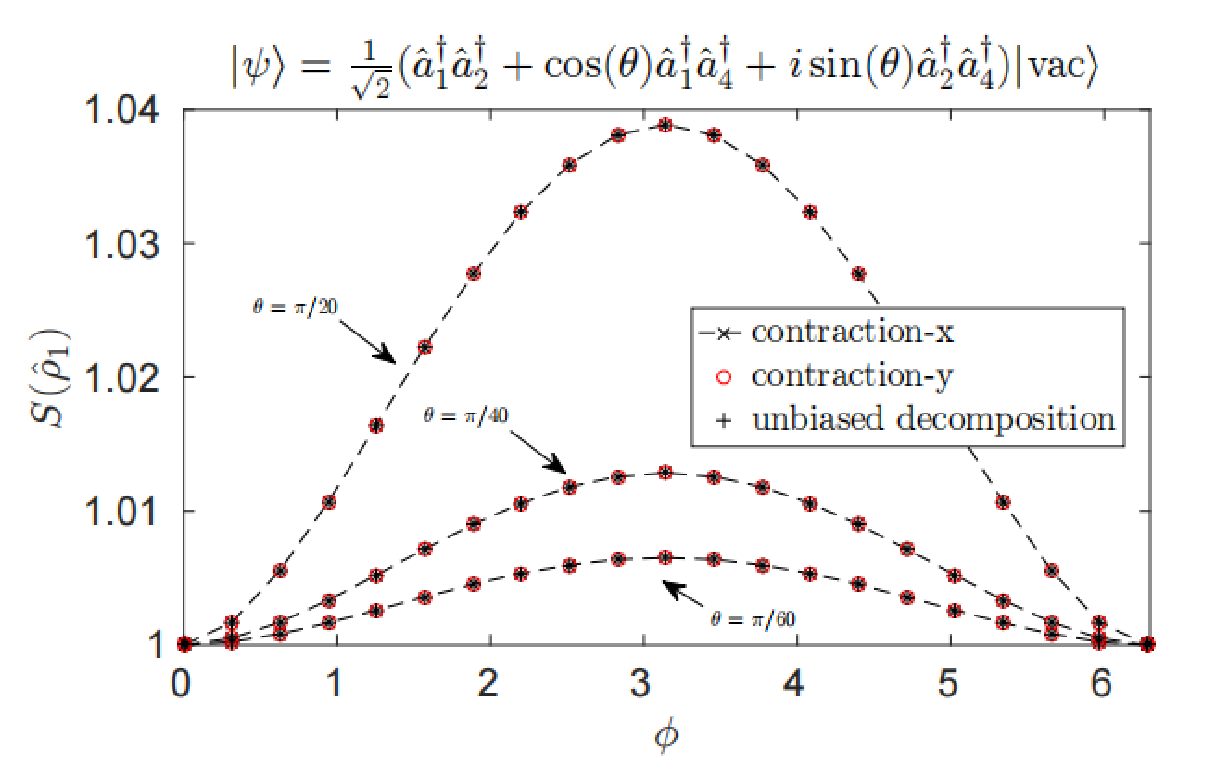
Figure 3: The von Neumann entropy of the single particle state for different values of $\theta$ in the function of $\phi$. The label $x$ indicates partial trace according to Eq. (108), and the label $y$ indicates partial trace according to Eq. (109).

The entanglement behaviour varies in function of $\theta$ and $\phi$. The dependence in $\phi$ arises from the terms $\rho(1;4)$ and $\rho(4;1)$, for

$$\rho(1;4)=-i\sin(\theta)\bra{0}a_{1}a_{2}a_{1}^{\dagger}a_{2}^{\dagger}\outerproduct{0}{0}a_{4}a_{2}a_{2}^{\dagger}a_{4}^{\dagger}\ket{0}=i\sin(\theta)\exp(i\phi)\bra{0}a_{1}a_{1}^{\dagger}\outerproduct{0}{0}a_{4}a_{4}^{\dagger}\ket{0}=i\sin(\theta)\exp(i\phi).$$

Also, similarly, the term

$$\rho(4;1)=i\sin(\theta)\bra{0}a_{4}a_{2}a_{2}^{\dagger}a_{4}^{\dagger}\outerproduct{0}{0}a_{2}a_{1}a_{2}^{\dagger}a_{1}^{\dagger}\ket{0}=-i\sin(\theta)\exp(-i\phi)\bra{0}a_{4}a_{4}^{\dagger}\outerproduct{0}{0}a_{1}a_{1}^{\dagger}\ket{0}=-i\sin(\theta)\exp(-i\phi)$$

has dependence in $\phi$. Actually, the $\phi$ dependence in the coherence of the single-particle density matrices reflects its eigenvalues and consequently the entanglement. This dependence could be suppressed if the single-particle density matrix is already diagonal, after the partial trace, It would analogous to obtaining the Schmidt decomposition for anyonic fermions.

Considering now, one performs the permutation operation on $\ket{\psi_{\raisebox{0.0pt}{\tiny{$\theta$}}}}$, resulting

$$\mathcal{P}\ket{\psi_{\raisebox{0.0pt}{\tiny{$\theta$}}}}=\exp(-i\phi)\frac{1}{\sqrt{2}}\left(a_{2}^{\dagger}a_{1}^{\dagger}+\cos\theta a_{4}^{\dagger}a_{1}^{\dagger}+i\sin\theta a_{4}^{\dagger}a_{2}^{\dagger}\right)\ket{0},$$ (115)

it carries a global phase without any implication in the global density matrix. Although, the single particle state gets some local phases, resulting

$$\rho^{\raisebox{0.0pt}{\tiny{$\mathcal{P}$}}}_{\raisebox{0.0pt}{\tiny{$sp$}}}=\frac{1}{4}\left(\scalebox{0.65}{\mbox{$\displaystyle\begin{array}[]{cccc}1+\cos^{2}(\theta)&i\sin(\theta)\cos(\theta)&0&i\sin(\theta)e^{-i\phi}\\ -i\sin(\theta)\cos(\theta)&1+\sin^{2}(\theta)&0&\cos(\theta)\\ 0&0&0&0\\ -ie^{+i\phi}\sin(\theta)&\cos(\theta)&0&1\\ \end{array}$}}\right),$$ (120)

where $\rho^{\raisebox{0.0pt}{\tiny{$\mathcal{P}$}}}_{\raisebox{0.0pt}{\tiny{$sp$}}}=\sum_{k}a_{k}\mathcal{P}\outerproduct{\psi_{\raisebox{0.0pt}{\tiny{$\theta$}}}}{\psi_{\raisebox{0.0pt}{\tiny{$\theta$}}}}\mathcal{P}^{\dagger}a_{k}^{\dagger}$. Besides anyonic permutation relations result on different single-particle states, the von Neumann of the single-particle density matrices are the same, as shown in Fig. 3. The action of permutations acts as we are tracing out another particle, as shown in Eq. (108) and Eq. (109) the trace of one particle or another can add a phase due to the permutation of anyons particles. To see this, considering the terms that have a dependence in $\phi$ in the single-particle density matrix, we will apply the partial trace as calculated Eq. (109) for the state Eq. (104). For the element

$$\rho_{\raisebox{0.0pt}{\tiny{$sp$}}}(1;4) =-i\sin(\theta)\bra{0}a_{1}\exp(i\phi(\epsilon_{21}+\epsilon_{42}))a_{2}a_{1}^{\dagger}a_{2}^{\dagger}\outerproduct{0}{0}a_{4}a_{2}a_{2}^{\dagger}a_{4}^{\dagger}\ket{0}$$ (121)

$$=i\sin(\theta)\exp(-i\phi)\bra{0}a_{1}a_{1}^{\dagger}\outerproduct{0}{0}a_{4}a_{4}^{\dagger}\ket{0}$$

$$=i\sin(\theta)\exp(-i\phi)=\rho^{\raisebox{0.0pt}{\tiny{$\mathcal{P}$}}}_{\raisebox{0.0pt}{\tiny{$sp$}}}(1;4).$$

And the term

$$\rho_{\raisebox{0.0pt}{\tiny{$sp$}}}(4;1) =i\sin(\theta)\bra{0}a_{4}\exp(i\phi(\epsilon_{24}+\epsilon_{12}))a_{2}a_{2}^{\dagger}a_{4}^{\dagger}\outerproduct{0}{0}a_{2}a_{1}a_{2}^{\dagger}a_{1}^{\dagger}\ket{0}$$ (122)

$$=-i\sin(\theta)\exp(i\phi)\bra{0}a_{4}a_{4}^{\dagger}\outerproduct{0}{0}a_{1}a_{1}^{\dagger}\ket{0}$$

$$=-i\sin(\theta)\exp(i\phi)=\rho^{\raisebox{0.0pt}{\tiny{$\mathcal{P}$}}}_{\raisebox{0.0pt}{\tiny{$sp$}}}(4;1).$$

We show that in this way that the terms $\rho^{\raisebox{0.0pt}{\tiny{$\mathcal{P}$}}}_{\raisebox{0.0pt}{\tiny{$sp$}}}(1;4)$ and $\rho^{\raisebox{0.0pt}{\tiny{$\mathcal{P}$}}}_{\raisebox{0.0pt}{\tiny{$sp$}}}(4;1)$ of the single-particle density matrix of the state with permutation Eq. (120) are obtained tracing out the particle (y) instead of the particle (x) of the state Eq. (104).

However, applying the fractional Jordan-Wigner transform (FJWT) in the state of the Eq. (104)

$$J\ket{\psi_{\raisebox{0.0pt}{\tiny{$\theta$}}}}=\exp(-i\phi)\frac{1}{\sqrt{2}}\left(f_{1}^{\dagger}f_{2}^{\dagger}+\cos\theta f_{1}^{\dagger}f_{4}^{\dagger}+i\sin\theta f_{2}^{\dagger}f_{4}^{\dagger}\right)\ket{0},$$ (123)

and after tracing out one particle we get the following single particle density matrix

$$\rho_{\raisebox{0.0pt}{\tiny{$sp$}}}^{\raisebox{0.0pt}{\tiny{$f$}}}=\frac{1}{4}\left(\scalebox{0.65}{\mbox{$\displaystyle\begin{array}[]{cccc}1+\cos^{2}(\theta)&i\sin(\theta)\cos(\theta)&0&i\sin(\theta)\\ -i\sin(\theta)\cos(\theta)&1+\sin^{2}(\theta)&0&\cos(\theta)\\ 0&0&0&0\\ -i\sin(\theta)&\cos(\theta)&0&1\\ \end{array}$}}\right),$$ (128)

it is independent of $\phi$. The single-particle density matrix is obtained through partial trace $\rho^{\raisebox{0.0pt}{\tiny{$f$}}}_{\raisebox{0.0pt}{\tiny{$sp$}}}=\sum_{k}\bra{0}f_{k}\outerproduct{\psi_{\raisebox{0.0pt}{\tiny{$\theta$}}}}{\psi_{\raisebox{0.0pt}{\tiny{$\theta$}}}}f_{k}^{\dagger}\ket{0}$, the partial trace is independent of the particles being trace out, such that for tracing out particle x

$$\rho_{y}(i_{2};j_{2})=\bra{\textrm{vac}}f_{i_{2}}\left(\sum_{i_{1}}f_{i_{1}}\outerproduct{\psi}{\psi}f^{\dagger}_{i_{1}}\right)f^{\dagger}_{j_{2}}\ket{\textrm{vac}}.$$ (129)

And tracing out particle y we obtain

$$\rho_{x}(i_{1};j_{1})=\bra{\textrm{vac}}-f_{i_{1}}\left(\sum_{i_{2}}f_{i_{2}}\outerproduct{\psi}{\psi}f^{\dagger}_{i_{2}}\right)-f^{\dagger}_{j_{1}}\ket{\textrm{vac}}=\bra{\textrm{vac}}f_{i_{1}}\left(\sum_{i_{2}}f_{i_{2}}\outerproduct{\psi}{\psi}f^{\dagger}_{i_{2}}\right)f^{\dagger}_{j_{1}}\ket{\textrm{vac}}=\rho_{y}(i_{2};j_{2}).$$ (130)

Also, the permutation operation on $J(\mathcal{P}\ket{\psi_{\raisebox{0.0pt}{\tiny{$\theta$}}}})$ only gives a minus sign resulting

$$J(\mathcal{P}\ket{\psi_{\raisebox{0.0pt}{\tiny{$\theta$}}}})=-\exp(-i\phi)\frac{1}{\sqrt{2}}\left(f_{2}^{\dagger}f_{1}^{\dagger}+\cos\theta f_{4}^{\dagger}f_{1}^{\dagger}+i\sin\theta f_{4}^{\dagger}f_{2}^{\dagger}\right)\ket{0},$$ (131)

the minus sign does not change the single-particle density matrix, because does not affect the density matrix of the global state. Furthermore, the partial trace for fermions does not generate phases because it is independent of the ordering of the particles, then the single-particle density matrices are independent of $\phi$ and the permutations. Now, for fermions the term

$$\rho_{\raisebox{0.0pt}{\tiny{$sp$}}}^{\raisebox{0.0pt}{\tiny{$f$}}}(1;4)=-i\sin(\theta)\bra{0}f_{1}f_{2}f_{1}^{\dagger}f_{2}^{\dagger}\outerproduct{0}{0}f_{4}f_{2}f_{2}^{\dagger}f_{4}^{\dagger}\ket{0}=i\sin(\theta)\bra{0}f_{1}f_{1}^{\dagger}\outerproduct{0}{0}f_{4}f_{4}^{\dagger}\ket{0}=i\sin(\theta),$$

and the term

$$\rho_{\raisebox{0.0pt}{\tiny{$sp$}}}^{\raisebox{0.0pt}{\tiny{$f\mathcal{P}$}}}(1;4)=-i\sin(\theta)\bra{0}f_{1}f_{2}f_{2}^{\dagger}f_{1}^{\dagger}\outerproduct{0}{0}f_{2}f_{4}f_{2}^{\dagger}f_{4}^{\dagger}\ket{0}=i\sin(\theta)\bra{0}f_{1}f_{1}^{\dagger}\outerproduct{0}{0}f_{4}f_{4}^{\dagger}\ket{0}=i\sin(\theta)=\rho_{\raisebox{0.0pt}{\tiny{$sp$}}}^{\raisebox{0.0pt}{\tiny{$f$}}}(1;4).$$

The eigenvalues of the single-particle density matrix in the fermionic representation are $\omega_{\mu}=\{1/2,1/2,0,0\}$, so the state in Eq. (128) is not entangled according to Slater decomposition Schliemann et al. (2001), since it has Slater rank equals to one. The single particle density matrices of the Eq.(114) and Eq. (120) present a von Neumann entropy dependent on $\phi$ and $\theta$ as shown in Fig. 3, while in the fermionic representation, the von Neumann entropy is equal to one independently of values of $\phi$ and $\theta$. Using Theorem B.1 we know that the state in the fermionic representation after the application of the Slater decomposition can be mapped, with inverse FJWT, to a state of anyons with the same coefficients. Therefore, the Schmidt coefficients of anyons are equal to $\omega_{\mu}$, independently of $\phi$ and $\theta$, such that the state in Eq. (104) is not entangled for all $\phi$ and $\theta$.