Kinetic Models of Wealth Distribution Having Extreme Inequality: Numerical Study of Their Stability Against Random Exchanges

Abstract

In view of some persistent recent reports on a singular kind of growth of the world wealth inequality, where a finite (often handful) number of people tend to possess more than the wealth of the planet’s 50% population, we explore here if the kinetic exchange models of the market can ever capture such features where a significant fraction of wealth can concentrate in the hands of a countable few when the market size $N$ tends to infinity. One already existing example of such a kinetic exchange model is the Chakraborti or Yard-Sale model, where (in absence of tax redistribution etc) the entire wealth condenses in the hand of one (for any value of $N$), and the market dynamics stops. With tax redistribution etc, its steady state dynamics have been shown to have remarkable applicability in many cases of our extremely unequal world. We show here that another kinetic exchange model (called here the Banerjee model) has intriguing intrinsic dynamics, by which only ten rich traders or agents possess about 99.98% of the total wealth in the steady state (without any tax etc like external manipulation) for any large value of $N$. We will discuss in some detail the statistical features of this model using Monte Carlo simulations. We will also show, if the traders each have a non-vanishing probability $f$ of following random exchanges, then these condensations of wealth (100% in the hand of one agent in the Chakraborti model, or about 99.98% in the hands ten agents in the Banerjee model) disappear in the large $N$ limit. We will also see that due to the built-in possibility of random exchange dynamics in the earlier proposed Goswami-Sen model, where the exchange probability decreases with an inverse power of the wealth difference of the pair of traders, one did not see any wealth condensation phenomena. These aspects of the statistics of these intriguing models have been discussed here.

I INTRODUCTION

The first successful theory of classical many-body physics or classical condensed matter systems has been about one and a quarter centuries old kinetic theory of the (classical) ideal gas, composed of Avogadro number (about $10^{23}$) order constituent atoms or molecule (each following Newtonian dynamics). It remains still a robust, versatile and extremely successful foundation of classical many-body physics. Social systems, economic markets in particular, are intrinsically many-body dynamical systems composed of a lesser number of constituents (order of $10^{2}$ for a village market to the order of $10^{10}$ for a global market). One Robinson Crusoe in an island can not develop a market or a society for that matter and markets are intrinsically many-body systems. It is no wonder that the kinetic exchange of money or wealth models had therefore been conjectured early on (e.g., by Saha and Srivastava Saha1931 in 1931, Mandelbrot Mandelbrot1960 in 1960) and resurrected recently (e.g., by Chakrabarti and Marjit Chakrabarti1995 in 1995, Dragulecu and Yakovenko Dragulescu2000 in 2000, Chakraborti and Chakrabarti Chakraborti2000 in 2000, Chatterjee, Chakrabarti and Manna Chatterjee2004a in 2004).

The kinetic exchange models of trades and their statistics have been quite successful in capturing several realistic features of wealth distributions among the agents in the societies (see e,g., Yakovenko2009 ; Chakrabarti2013 ). The beneficial effects of the agent’s saving propensity in reducing the social inequality has been studied extensively Chakraborti2000 ; Chatterjee2004a ; Chakrabarti2013 . The choice of the poorest trader as mandatory in each trade (the other trade partner being randomly chosen) leads to the remarkable self-organized poverty line, below which none remains in the steady state (see e.g., Pianegonda2004 ; Iglesias2010 ; Ghosh2011 ; Paul2022 ). This model was inspired by some crucial observations by the economists (see e.g., Iglesias2010 ) and suggests the built-in (self-organized) remedies for reducing social inequality. Though it must be admitted, such intriguing self-organizing properties of the kinetic exchange models have not been investigated extensively yet.

Contrarily, the recent focus has moved to the unusual rate of growth of social inequality in the post world war II period (see e.g., Pickety2014 ; Iglesias2021 ; Danial2022 ; Banerjee2023 ), which in some countries seem to have crossed significantly above the 80-20 Pareto limit and have reached a steady state with 87% percent wealth accumulated in the hands of 13% people. This has indeed been argued, following an analogy with the inequality index values for the avalanche burst statistics in self-organized sand-pile models near their respective critical points, to be the natural limit in all social competitive situations, where the welfare mechanisms (helping those who fail to participate properly in such self-organizing dynamics) are either absent or removed (see e.g., a recent review Banerjee2023 ).

Although the Pareto-like inequality mentioned above where a small fraction of people (say 13%) possess a large fraction (say 87%) of wealth, can already be devastating, more annoying kind of inequalities are being reported recently. For example, the Oxfam Report Oxfam2020 of January, 2020 in Davos said “The world’s 2,153 billionaires have more wealth than the 4.6 billion people who makeup 60 percent of the planet’s population.” In other words, a handful number (about $10^{3}$) of rich people possess more than about 60% (or $10^{9}$ order) poor people’s wealth of this planet. This dangerous trend in the world as a whole, is repeatedly mentioned in various recent reports.

The Pareto-type inequality mentioned above have long been investigated (see e.g., Chatterjee2004a ; Chatterjee2007 ) using the kinetic exchange models with non-uniform saving propensities of the traders (see e.g., Chakrabarti2013 , Pareschi2014 for reviews). One may naturally ask the question, does the kinetic exchange theory allow for possible models where only a handful of traders (say, about 10 in number) possess a significant fraction (say, above 50%) of the total wealth considered in the model, even when its population $N$ tends to infinity?

The answer is yes. The Chakraborti model Chakraborti2002 , widely known today as the Yard-Sale model, starting with Hayes2002 , have attracted a lot of attention (see e.g., Cardoso2023 ; Boghosian2019 ; Julian2022 ). In its barest form Chakraborti2002 in the Chakraborti model (called C-model here), two randomly chosen traders at any point of time come and participate in an exchange trade when the richer one saves the excess over the poorer’s wealth and goes for a random exchange of the total available wealth (double of the poorer’s). The slow but inevitable attractor fixed point of the trade dynamics arrive when all wealth ends up in the hand of just one trader, no matter how big the population ($N$) is. Because of the particular form of savings during any trade, whenever one becomes pauper, nobody trades with him and gradually all condense to that state where one trader acquires the entire wealth and the trade dynamics stop (see also Cardoso2023 ). External perturbations like regular redistribution of tax collections by the central government (or any non-playing agent) can help relieving Boghosian2019 ; Julian2022 the condensation phenomenon and this seems to fit well with many observed situations Boghosian2019 . We will show here numerically that if each of the traders has a finite probability ($f$) of playing Dragulecu and Yakovenko (DY) Dragulescu2000 type random exchanges, then for any $f>0$, the condensation of wealth in the hand of one trader disappear and the steady state distribution of wealth becomes exponentially decreasing, as in the DY model.

In the Goswami-Sen (or GS) model Goswami2014 , one considers a kinetic exchange mechanism where the interaction (trade) probability among the trade partners ($i$ and $j$) decreases with their wealth difference ($|m_{i}-m_{j}|$) at that instant of trading (time), following a power law ($|m_{i}-m_{j}|^{-\alpha}$). Of course, for $\alpha$ = 0, the model reduces to that of DY. Their numerical results showed that for $\alpha$ values less than about 2.0, the steady-state wealth distribution among the traders are still DY-like (exponentially decaying with increasing wealth). For higher values (beyond 2.0) of $\alpha$, power-law (Pareto-law) decays occur. No condensation of wealth in the hands of a finite number of traders or agents are observed, because of the inherent DY-like exchange probability in the dynamics of the model (checked by extrapolating with $N$ the fraction of total wealth possessed in the steady state by the richest ten traders).

We finally consider here a seemingly natural version of the kinetic exchange model, called here the Banerjee (B) model Banerjee2021 , where the intrinsic dynamics of the model lead to another extreme kind of inequality in the steady state in the sense that precisely ten traders (out of the $N$ traders in the market; $N\rightarrow\infty$) possess (99.98 $\pm$ 0.01)% of the total wealth. These fortunate traders are not unique and their fortune does not last for long (residence time on average is about 66 time units with the most probable value around 25 time units, counted in units of $N$ trades or exchanges, for any value of $N$) and it decreases continuously with increasing fraction ($f$) of random trades or interactions. Unlike in the Chakraborti or Yard-Sale model Chakraborti2002 ; Hayes2002 , where the dynamics stops after the entire wealth goes to one (unless perturbed externally), here the trade dynamics continue with the total wealth circulating only within a handful (about ten) traders in the steady state. In this model, after each trade, the traders are ordered from lowest wealth to highest and each of the traders trade only with their nearest-in-wealth traders, richer or poorer compared to own, with equal probability. Even if by chance the entire wealth goes to one trader, the dynamics of random exchanges do not stop in this model as all the paupers become the only nearest neighbors (wealth-wise) of this trader and random exchange among them occurs! The process continues. Apart from the steady state wealth distributions and most probable wealth amounts of the top few rich traders, we will show that in this model the condensation of almost the entire (99.98%) wealth occurs in the hands of 10 traders (no matter how big $N$ is). We will show here again that this condensation disappears when a finite fraction $f$ of time each of the traders go for DY type random exchanges, and eventually the DY-type exponentially decaying wealth distribution sets-in, after a power law region for low values of $f$.

II MODELS and NUMERICAL STUDIES FOR THEIR STATISTICS

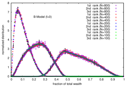
Figure 1: Distributions of the fraction of total wealth ($M=N$) ending up in the hands of the richest three traders. The error estimation is based on 10 runs. The typical errors in the distribution of wealth are seen to grow with $N$ near the most-probable value of the wealth fraction and are indicated for $N$ = 800 for all the three traders. Far away from the most-probable values, the errors are less than the data point symbol sizes.

We study here numerically the statistical features of the three kinetic exchange models introduced in the Introduction. We begin with the B (Banerjee Banerjee2021 ) model. Next, we consider the C (Chakraborti, or Yard Sale) model Chakraborti2002 ; Hayes2002 and then the GS (Goswami-Sen) model Goswami2014 . In order to explore the stability of the condensation of wealth feature in these models, we study the steady-state wealth distributions $P(m)$ in each of these models and the fraction of total wealth concentrated in the hands of a few (say ten) traders or agents (whenever meaningful), allowing each trader to have a nonvanishing probability $f$ (the faction of tradings or times) to go for DY (Dragulecu and Yakovenko Dragulescu2000 ) type random exchanges.

Most of the numerical (Monte Carlo) studies of the dynamics of these models are studied with four sets of numbers $N$ of the agents or traders: $N$ = 100, 200, 400, and 800 and at each time step $t$, the dynamics runs over all the $N$ order traders. We consider total money ($M$), to be distributed among the agents is equal to $N$ and we denote the money of any agent $i$ at time $t$ by $m_{i}(t)$ and, as such $M=\sum_{i}m_{i}(t)=N$. When the steady state is reached after the respective relaxation times when the average quantities do not change with time (relaxation time typically much less than $10^{5}$ trades/interactions for the $N$ values considered here), the statistical quantities are evaluated from averages over $10^{5}$ post-relaxation time steps or so.

II.1 Banerjee model results

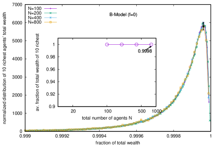
Figure 2: Distribution of the total wealth fraction possessed by the ten richest (at any time in the steady state and for different $N$ values). The inset shows that the average of this total wealth fraction of the ten richest (for any time and any value of $N$) in the steady state is very close to 0.9998. It may be noted, although the wealth share fractions of the richest ten traders have considerable fluctuations (see Fig. 1), the sum total of their wealth fractions have hardly any fluctuation (much less than the symbol size in the inset). The error estimation is based on 10 runs. The typical error in the distribution of total wealth of the ten richest are seen to be more than the data point symbol sizes only near the most-probable value, where it is indicated.

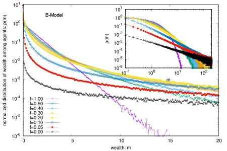
Figure 3: Wealth distribution $P(m)$ among all the agents against the wealth $m$ in the B model for different probability $f$ of DY random exchanges. Note that the fluctuations appear to grow more for the lower values of the distribution of wealth due to the log scale used in the y-axis.

In this B-model, when the DY fraction ($f$) is set equal to zero, no wealth distribution $P(m)$ across the population is meaningful, because of wealth condensation in the hands of a few. We first study the distributions (see Fig. 1) of total wealth fraction in the hands of the richest three. Note, these three are not unique, and once they become so rich, their residence time (in unit of $N$) is finite (about 66) and in case these positions are lost, the return time also is finite.

Though the distributions of the total wealth fraction in the hands of the few richest (shown in Fig. 1) are rather wide (each one spread over more than 30% of the total wealth and does not $N$), the distribution of the total wealth fraction possessed by the ten richest (at any time in the steady state) is extremely narrow and spreads over 0.1% only (see Fig. 2). At any time in the steady state its value is much more robust in this B model (with $f$ = 0) and its value is less than unity, but very close to 0.9998.

Next, we consider the B model with a nonvanishing probability $f$ of each trader to follow DY trades or exchanges. We see, immediately, the wealth condensation disappears and with increasing values of $f$, the wealth gets Boltzmann (exponentially) distributed among all the agents (see Fig. 3), starting with Pareto-like power law distribution for lower values of $f$ (see the inset of Fig. 3). Indeed, when we consider the limiting values (for large $N$) of the average fraction of total wealth ($M=N$) possessed by the ten richest traders in the steady state, they all seem to vanish (see Fig. 4) for any non-zero value of $f$ (and remains a constant 0.9998 for $f$ = 0, the pure B model).

For the wealth condensation in B-model (with $f$ = 0), we show next in Fig. 5(a), the distribution of residence-time (in unit of $N$) of the 10 fortunate traders and (in the inset) the variation of the most probable and average values of the residence-time ($\tau$, in unit of $N$). For the same model with $f$ = 0, we show in Fig. 5(b) the distribution of return-time to fortune (become one of the 10 richest starting from the 20th rank) and (in the inset) the variation of the most probable and average values of the residence-time with market size $N$.

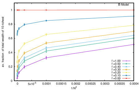
Figure 4: To get the limiting values (for large $N$) of the average fraction of total wealth ($M=N$) possessed by the ten richest traders in the steady state, we plot the fraction against $1/N^{2}$ (as with DY type trades each of N traders interacts with (N - 1 other trader). The extrapolated values all seem to approach zero for any non-zero value of $f$ (but remains a constant 0.9998 for $f$ = 0, as in the pure B model). The error estimation is based on 10 runs. Typical sizes of error bars are indicated.

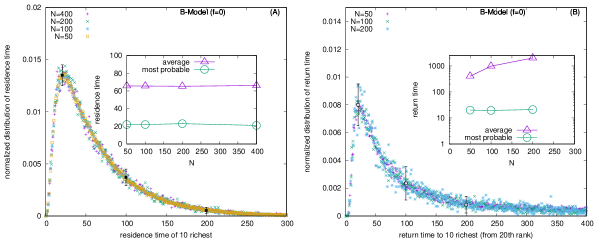
Figure 5: (a) The distribution of residence-time (in units of $N$) of the 10 fortunate traders and (in the inset) the variation of the most probable and average values of the residence time. (b) The distribution of return-time to fortune (become one of the 10 richest, starting from the 20th rank) and (in the inset) the variation of the most probable and average values of the return-time (in units of $N$). The error estimation is based on 10 runs. The typical errors in the distribution of both the residence and return times are seen to grow with $N$ near the most-probable values of the respective quantities and are indicated for $N$ = 400 here, when they are bigger than the symbol sizes.

II.2 Chakraborti or Yard-Sale model results

The C Model or Yard sale model is well-studied. However, in order to check the stability of the condensation of wealth (entire money $M=N$ going to the hand of one trader only, we added a nonvanishing probability $f$ of each trader to follow DY trades or exchanges. We see, immediately, the wealth condensation disappears for any $f>0$ (see Fig. 6) and the wealth gets distributed in the Boltzmann form (exponentially decaying with increasing wealth) among all the agents. The inset shows that for any nonzero value of $f$, the steady state wealth distribution is exponentially decaying (and there is a power law region) in this extended model C. Also, when we consider the limiting values (for large $N$) of the average fraction of total wealth ($M=N$) possessed by the ten richest traders the steady state (see Fig. 7), they all seem to vanish from the unit value in the original C model (with $f=0$) for any non-zero value of $f$.

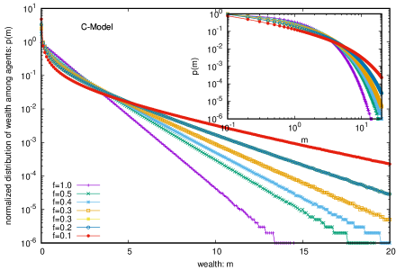
Figure 6: Wealth distribution $P(m)$ among all the agents against the wealth $m$ in the C model for different probability $f$ of DY random exchanges. Note that the fluctuations appear to grow more for the lower values of the distribution due to the log scale used in the y-axis.

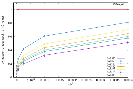
Figure 7: The limiting values (for large $N$) of the average fraction of total wealth ($M=N$) possessed by the ten richest traders in the the steady state of the C model with $f$ fraction of DY-like trades. For $f=0$, the entire money goes to one agent and the other nine agents contribute nothing. When we plot the fraction against $1/N^{2}$ (as with DY type trades each of N traders interacts with $(N-1)$ other traders), the extrapolated values all seem to approach zero for any non-zero value of $f$. The error estimation is based on 10 runs. Typical sizes of error bars are indicated.

II.3 Goswami-Sen model results

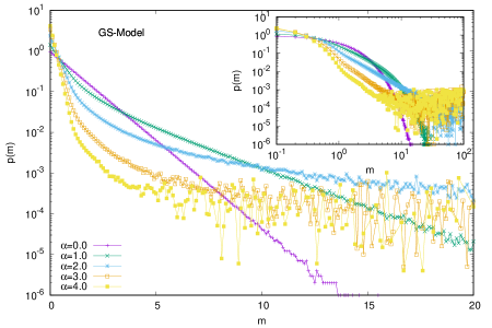
Figure 8: Wealth distribution $P(m)$ among all the agents against the wealth $m$ in the GS model for different values of $\alpha$. Note that the fluctuations appear to grow more for the lower values of the distribution due to the log scale used in the y-axis.

Here the interaction (trade) probability among the trade partners ($i$ and $j$) decreases with their wealth difference ($|mi–mj|$) at that instant of trading (time), following a power law ($|mi–mj|^{-\alpha}$). As such in the GS model, there is always a finite (but small) probability of random exchanges. We do not need to consider the additional fraction of DY interaction in this model. Of course, for $\alpha$ = 0, the model reduces to that of DY. Our numerical results confirm (see Fig. 8) that for $\alpha$ values less then about 2.0, the steady-state wealth distribution among the traders are still DY-like (exponentially decaying). For higher values (beyond 2.0) of $\alpha$, power-law (Parto-like) decays occur (but no condensation of wealth). Though the model leads to extreme inequality, there is no condensation of wealth in the hands of a few traders for any (larger) value of $\alpha$. In order to check that we studied again the average fraction of total wealth ($M=N$) possessed by the ten richest traders in the steady state of the GS model with $\alpha$. When we plot the fraction against $1/N^{2}$ (see Fig. 9), the extrapolated values of the fraction all seem to approach zero for any non-zero value for any of the $\alpha$ values considered.

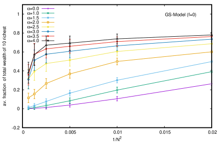
Figure 9: Plot of the fraction of total wealth ($M=N$) against $1/N^{2}$ for different values of $\alpha$ in the GS model. The extrapolated (with $N$) values of the fraction all seem to approach zero for any non-zero value of $\alpha$. The error estimation is based on 10 runs. Typical sizes of error bars are indicated.

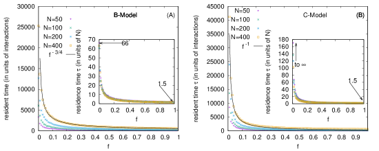
Figure 10: The DY fraction $f$ dependence of the bare residence time (in units of interactions or exchanges) at different $N$ values for B-model (Fig. 10a) and for C-model (Fig. 10b) are shown. Their power law fits with $f$ for $N$ = 400 are shown (for other $N$ vales, the respective prefactors change linearly with $N$). The insets show the $f$ dependence of the residence-time $\tau$ (in units of $N$). Note that the limiting values of $\tau$ at $f$ = 0 is about 66 for the B-model, while it goes to infinity for the C-model.

III SUMMARY and DISCUSSION

In view of the observed extreme income or wealth inequalities in society, the suitability of the kinetic exchange models Chakrabarti2013 to capture them, at least qualitatively, have been investigated here. We distinguish between two types of such extreme inequalities: One (Pareto) type Banerjee2023 where a small fraction (typically 13%) of the population possess about 87% of the total wealth (following a power law distribution) of the respective country. The other more recently observed (and reported by Oxfam Oxfam2020 ) truly extreme nature of income and wealth inequalities worldwide, where only a handful number (say a few hundreds to thousands) of super-rich people of the world accumulate more than the total wealth of 50 to 60 percent poor people.

Several kinetic exchange models (see e.g, Chatterjee2004a ; Chakrabarti2013 ) have been developed to analyze Pareto type of inequalities. We have investigated here the statistics of some kinetic exchange models where, even in the $N$ going to infinity limit, only one person can grab the entire wealth (as in the Yard-sale or Chakraborti or C model Chakraborti2002 ; Hayes2002 ), or only 10 people can accumulate about 99.98% of the total wealth (as in the Banerjee or B model Banerjee2021 , see Fig. 2). We investigate how these extreme inequalities in these kinetic models get softened to the Dragulescu-Yakovenko (DY) Dragulescu2000 type exponentially decaying wealth distributions among all the traders or agents, when the traders each have a non-vanishing probability $f$ of DY-type random exchanges. These condensations of wealth (100% in the hand of one agent in the C model Chakraborti2002 , or about 99.98% in the hands of ten agents in the B model) then disappear in the large $N$ limit (clearly seen when extrapolated against $1/N^{2}$, as in DY type random exchanges, each of $N$ agents interact or exchange with all others; see Figs. 4 and 7). We also showed that due to the built-in possibility of DY-type random exchange dynamics in the Goswami-Sen or GS model Goswami2014 , where the exchange probability decreases with an inverse power of the wealth difference of the pair of traders, one does not see any wealth condensation phenomena. In both GS and B model (with $f>0$ fraction DY interactions or exchanges) no wealth condensation occurs, though strong Pareto-type power-law wealth distribution $P(m)$ or inequalities occur for large values of $\alpha$ and smaller values of $f$ in GS and B models respectively (see Figs. 3 and 8). For the wealth condensation in the B model, for $f$ = 0, we additionally find that the fortunate top ten traders are not unique and their fortune does not last for long (residence-time $\tau$ to fortune on average is about 66 time units with its most probable value around 25 time units, when counted in units of $N$ trades or exchanges; see Fig. 5a). The most probable ‘return-time’ to such a fortune (of the 20th rank holder to come within the group of fortunate 10), is found to be about 20 (again in units of $N$; see Fig. 5b). It may be noted that with $f=0$, in the C-model, the residence-time $\tau$ is infinity for the only fortunate one accumulating the entire wealth in the system. Indeed with increasing values of DY fraction $f$, the values of $\tau$ in both the cases decrease rapidly (see Fig. 10), following inverse power laws with $f$. We further note, for $f$ = 0 in the B-model near the most-probable values of the wealth fractions (Figs. 1 and 2) and residence or return times (Fig. 5), the fluctuations tend to grow with $N$, indicating a possible divergence there in the macroscopic limit of $N$. We plan to explore its significance later.

Our studies for the B, C, and GS kinetic exchange models, using Monte Carlo techniques code , suggest that the potential condensation type extreme inequality can disappear in all of them if a non-vanishing probability of random exchanges are allowed, and converge to Pareto-type power law inequality (for B and GS model) which in turn converges to Gibbs like (exponentially decaying) wealth distribution for larger values of $f$ in the B model, smaller values of $\alpha$ in the GS model, or any values of $f>0$ in the C model. These observations may help to formulate public welfare policies.

References

- (1) M. N. Saha and B. N. Srivastava, B.N. A Treatise on Heat, p. 105, Indian Press: Allahabad, India (1931)
- (2) Mandelbrot, B. B., The Pareto-Levy law and the distribution of income. International Economic Review, 1, 79-106 (1960)
- (3) B. K. Chakrabarti and S. Marjit, Self-organisation and complexity in simple model systems: Game of life and economics, Indian Journal of Physics, 69B, 681–698 (1995).
- (4) A. Dragulescu, V. M. Yakovenko, Statistical mechanics of money. European Physical Journal B - Condensed Matter and Complex Systems 2000, 17, 723–729. (2000)
- (5) A. Chakraborti and Chakrabarti, B.K. Statistical mechanics of money: How saving propensity affects its distribution, European Physical Journal B - Condensed Matter and Complex Systems, 17, 167–170 (2000)
- (6) A. Chatterjee, B. K. Chakrabarti and S. S. Manna, Pareto law in a kinetic model of market with random saving propensity. Physica : Statistical Mechanics and its Applications, 335, 155–163 (2004)
- (7) V. M. Yakovenko and J. B. Rosser, Statistical mechanics of money, wealth, and income, Rev. Mod. Phys. 81, 1703 (2009)
- (8) B. K. Chakrabarti, A. Chakraborti, S. R. Chakravarty and Chatterjee, Econophysics of Income and Wealth Distributions, Cambridge Univ. Press (2013)
- (9) Pianegonda, S.; Iglesias, J.R. Inequalities of wealth distribution in a conservative economy, Physica A, 42, 193–199 (2004)
- (10) J. R. Iglesias, How simple regulations can greatly reduce inequalities, Science and Culture, 76, 437–443 (2010) [arXiv:1007.0461]
- (11) A. Ghosh, U. Basu, A. Chakraborti, and B. K. Chakrabarti, Threshold-induced phase transition in kinetic exchange models. Physical Review E, 83(6):061130 (2011
- (12) S. Paul et al., Kinetic Exchange Income Distribution Models with Saving Propensities: Inequality Indices and Self-Organised Poverty Level, Philosophical Transactions of the Royal Society A, 380, 20210163 (2022)
- (13) T. Pickety, Capital in Twenty First Century, Harvard University Press, Massachusetts (2014)
- (14) J. R. Iglesias, B.-H. F. Cardoso and S. Gonçalves, Inequality, a scourge of the XXI century, Communications in Nonlinear Science and Numerical Simulation, 95, 105646 (2021)
- (15) L. Danial and V. M. Yakovenko, Physics-inspired analysis of the two-class income distribution in the USA in 1983–2018, Phil. Trans. R. Soc. A, 380, 20210162 (2022) [http://doi.org/10.1098/rsta.2021.0162]
- (16) S. Banerjee, S. Biswas, B. K. Chakrabarti, A. Ghosh and M Mitra, Sandpile Universality in Social Inequality: Gini and Kolkata Measures. Entropy, 25, 735 (2023) [https://doi.org/10.3390/e25050735]
- (17) Oxfam International Report (2020) [https://www.oxfam.org/en/press-releases/worlds-billionaires-have-more-wealth-46-billion-people]
- (18) A. Chatterjee and B. K Chakrabarti. Kinetic exchange models for income and wealth distributions. The European Physical Journal B, 60, 135–149 (2007)
- (19) L. Pareschi and G. Toscani, Interacting Multiagent Systems, Oxford University Press, Oxford (2014)
- (20) A. chakraborti, Distributions of money in model markets of economy, International Journal of Modern Physics C, 13, 1315–1321 (2002)
- (21) B. Hayes, Follow the Money, American Scientist, 90, 400-405 (2002)
- (22) B.-H. F. Cardoso, S. Gonçalves and J. R. Iglesias, Why equal opportunities lead to maximum inequality? The wealth condensation paradox generally solved, Chaos, Solitons and Fractals, 168, 113181 (2023)
- (23) B. Boghosian, Is Inequality Inevitable?, Scientific American, 321, 70-77 (2019)
- (24) N. Julian, C. B.-H. F. Cardoso, L. M. Fabiana, S. Gonçalves and J. R. Iglesias, Study of taxes, regulations and inequality using machine learning algorithms, Philosophical Transactions of the Royal Society A, 380 20210165 (2022)
- (25) S. Goswami and P. Sen, Agent based models for wealth distribution with preference in interaction, Physica A: Statistical Mechanics and its Applications, 415, 514-524 (2014)
- (26) S. Banerjee, Role of Neighbouring Wealth Preference in Kinetic Exchange model of market, arXiv:2305.16238 (2023)
- (27) Code will be available from the corresponding author upon request.