Robust covariance estimation with missing values and cell-wise contamination

Abstract

Large datasets are often affected by cell-wise outliers in the form of missing or erroneous data. However, discarding any samples containing outliers may result in a dataset that is too small to accurately estimate the covariance matrix. Moreover, the robust procedures designed to address this problem require the invertibility of the covariance operator and thus are not effective on high-dimensional data. In this paper, we propose an unbiased estimator for the covariance in the presence of missing values that does not require any imputation step and still achieves near minimax statistical accuracy with the operator norm. We also advocate for its use in combination with cell-wise outlier detection methods to tackle cell-wise contamination in a high-dimensional and low-rank setting, where state-of-the-art methods may suffer from numerical instability and long computation times. To complement our theoretical findings, we conducted an experimental study which demonstrates the superiority of our approach over the state of the art both in low and high dimension settings.

1 Introduction

Outliers are a common occurrence in datasets, and they can significantly affect the accuracy of data analysis. While research on outlier detection and treatment has been ongoing since the 1960s, much of it has focused on cases where entire samples are outliers (Huber’s contamination model) (huberRobustEstimationLocation1964, ; tukeyNintherTechniqueLowEffort1978, ; hubertMinimumCovarianceDeterminant2018, ). While sample-wise contamination is a common issue in many datasets, modern data analysis often involves combining data from multiple sources. For example, data may be collected from an array of sensors, each with an independent probability of failure, or financial data may come from multiple companies, where reporting errors from one source do not necessarily impact the validity of the information from the other sources. Discarding an entire sample as an outlier when only a few features are contaminated can result in the loss of valuable information, especially in high-dimensional datasets where samples are already scarce. It is important to identify and address the specific contaminated features, rather than simply treating the entire sample as an outlier. In fact, if each dimension of a sample has a contamination probability of $\varepsilon$, then the probability of that sample containing at least one outlier is given by $1-(1-\varepsilon)^{p}$, where $p$ is the dimensionality of the sample. In high dimension, this probability can quickly exceed $50\%$, surpassing the breakdown point of many robust estimators designed for the Huber sample-wise contamination setting. Hence, it is crucial to develop robust methods that can handle cell-wise contaminations and still provide accurate results.

The issue of cell-wise contamination, where individual cells in a dataset may be contaminated, was first introduced in (alqallafPropagationOutliersMultivariate2009, ). However, the issue of missing data due to outliers was studied much earlier, dating back to the work of rubinInferenceMissingData1976 . Although missing values in a dataset are much easier to detect than outliers, they can lead to errors in estimating the location and scale of the underlying distribution (littleStatisticalAnalysisMissing2002, ) and can negatively affect the performance of supervised learning algorithms (josseConsistencySupervisedLearning2020, ). This motivated the development of the field of data imputation. Several robust estimation methods have been proposed to handle missing data, including Expectation Maximization (EM)-based algorithms (dempsterMaximumLikelihoodIncomplete1977, ), maximum likelihood estimation (jamshidianMLEstimationMean1999, ) and Multiple Imputation (littleStatisticalAnalysisMissing2002, ), among which we can find k-nearest neighbor imputation troyanskayaMissingValueEstimation2001 and iterative imputation buurenMiceMultivariateImputation2011 . Recently, sophisticated solutions based on deep learning, GANs yoonGAINMissingData2018 ; matteiMIWAEDeepGenerative2019 ; dongGenerativeAdversarialNetworks2021 , VAE maVAEMDeepGenerative2020 or Diffusion schemes zhengDiffusionModelsMissing2023 have been proposed to perform complex tasks like artificial data generation or image inpainting. The aforementioned references focus solely on minimising the entrywise error for imputed entries. Noticeably, our practical findings reveal that applying state-of-the-art imputation methods to complete the dataset, followed by covariance estimation on the completed dataset, does not yield satisfactory results when evaluating the covariance estimation error using the operator norm.

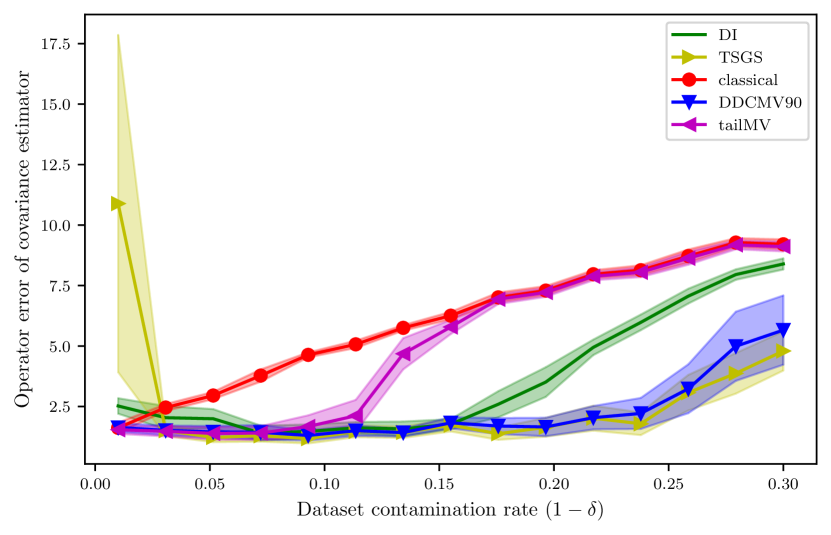
Estimator	Computation time		Matrix
	p=50	p=100	inversion
tailMV	$10^{-3}\pm 10^{-4}$	$10^{-2}\pm 10^{-3}$	no
DDCMV	$0.6\pm 10^{-3}$	$0.7\pm 0.007$	no
DI	$6\pm 0.5$	$74\pm 4$	yes
TSGS	$20\pm 0.2$	$200\pm 10$	yes

Figure 1: Left: Estimation error of the covariance matrix for $n=100$, $p=50$, $\mathbf{r}(\Sigma)=2$ under a Dirac contamination (tailMV and DDCMV are our methods). Here $\varepsilon=1$ and $\delta$ varies in $(0,1)$. Right: For each method, mean computation time (in seconds) over 20 repetitions and whether it uses matrix inversion. For $p=100$, we had to raise $r\left(\Sigma\right)$ to $10$ otherwise both DI and TSGS would fail due to numerical instability.

In comparison to data missingness or its sample-wise counterpart, the cell-wise contamination problem is less studied. The Detection Imputation (DI) algorithm of raymaekersHandlingCellwiseOutliers2020 is an EM type procedure combining a robust covariance estimation method with an outlier detection method to iteratively update the covariance estimation. Other methods include adapting methodology created for Huber contamination for the cell-wise problem, such as in danilovRobustEstimationMultivariate2012 or agostinelliRobustEstimationMultivariate2014 . In high dimensional statistics, however, most of these methods fail due to high computation time and numerical instability. Or they are simply not designed to work in this regime since they are based on the Mahalanobis distance, which requires an inversion of the estimated covariance matrix. This is a major issue since classical covariance matrix estimators have many eigenvalues close to zero or even exactly equal to zero in high-dimension. To the best of our knowledge, no theoretical result exists concerning the statistical accuracy of these methods in the cell-wise contamination setting contrarily to the extensive literature on Huber’s contamination abdallaCovarianceEstimationOptimal2023 .

Contributions. In this paper we address the problem of high-dimensional covariance estimation in the presence of missing observations and cell-wise contamination. To formalize this problem, we adopt and generalize the setting introduced in farcomeniRobustConstrainedClustering2014 . We propose and investigate two different strategies, the first based on filtering outliers and debiasing and the second based on filtering outliers followed by imputation and standard covariance estimation. We propose novel computationally efficient and numerically stable procedures that avoid matrix inversion, making them well-suited for high-dimensional data. We derive non-asymptotic estimation bounds of the covariance with the operator norm and minimax lower bounds, which clarify the impact of the missing value rate and outlier contamination rate. Our theoretical results also improve over louniciHighdimensionalCovarianceMatrix2014 in the MCAR and no contamination. Next, we conduct an experimental study on synthetic data, comparing our proposed methods to the state-of-the-art (SOTA) methods. Our results demonstrate that SOTA methods fail in the high-dimensional regime due to matrix inversions, while our proposed methods perform well in this regime, highlighting their effectiveness. Then we demonstrate the practical utility of our approach by applying it to real-life datasets, which highlights that the use of existing estimation methods significantly alters the spectral properties of the estimated covariance matrices. This implies that cell-wise contamination can significantly impact the results of dimension reduction techniques like PCA by completely altering the computed principal directions. Our experiments demonstrate that our methods are more robust to cell-wise contamination than SOTA methods and produce reliable estimates of the covariance.

2 Missing values and cell-wise contamination setting

Let $X_{1},\dots,X_{n}$ be $n$ i.i.d. copies of a zero mean random vector $X$ admitting unknown covariance operator $\Sigma=\mathbb{E}\left[X\otimes X\right]$, where $\otimes$ is the outer product. Denote by $X_{i}^{(j)}$ the $j$th component of vector $X_{i}$ for any $j\in[p]$. All our results are non-asymptotic and cover a wide range of configurations for $n$ and $p$ including the high-dimensional setting $p\gg n$. In this paper, we consider the following two realistic scenarios where the measurements are potentially corrupted.

Missing values.

We assume that each component $X_{i}^{(j)}$ is observed independently from the others with probability $\delta\in(0,1]$. Formally, we observe the random vector $Y\in\mathbb{R}^{p}$ defined as follows:

$$Y_{i}^{(j)}=d_{i,j}X_{i}^{(j)},1\leq i\leq n,1\leq j\leq p$$ (1)

where $d_{ij}$ are independent realisations of a bernoulli random variable of parameter $\delta$. This corresponds the Missing Completely at Random (MCAR) setting of rubinInferenceMissingData1976 . Our theory also covers the more general Missing at Random (MAR) setting in Theorem 2.

Cell-wise contamination.

Here we assume that some missing components $X_{i}^{(j)}$ can be replaced with probability $\varepsilon$ by some independent noise variables, representing either a poisoning of the data or random mistakes in measurements. The observation vector $Y$ then satisfies:

$$Y_{i}^{(j)}=d_{i,j}X_{i}^{(j)}+(1-d_{i,j})e_{i,j}\xi_{i}^{(j)},1\leq i\leq n,1\leq j\leq p$$ (2)

where $\xi_{i}^{(j)}$ are independent erroneous measurements and $e_{i,j}$ are i.i.d. bernoulli random variables with parameter $\varepsilon$. We also assume that all the variables $X_{i}$, $\xi_{i}^{(j)}$, $d_{i,j}$, $e_{i,j}$ are mutually independent. In this scenario, a component $X_{i}^{(j)}$ is either perfectly observed with probability $\delta$, replaced by a random noise with probability $\varepsilon^{\prime}=\varepsilon(1-\delta)$ or missing with probability $(1-\delta)(1-\varepsilon)$. Cell-wise contamination as introduced in alqallafPropagationOutliersMultivariate2009 corresponds to the case where $\varepsilon=1$, and thus $\varepsilon^{\prime}=1-\delta$.

In both of these settings, the task of estimating the mean of the random vectors $X_{i}$ is well-understood, as it reduces to the classical Huber setting for component-wise mean estimation. One could for instance apply the Tuker median on each component separately alqallafPropagationOutliersMultivariate2009 . However, the problem becomes more complex when we consider non-linear functions of the data, such as the covariance operator. Robust covariance estimators originally designed for the Huber setting may not be suitable when applied in the presence of missing values or cell-wise contaminations.

We study a simple estimator based on a correction of the classical covariance estimator on $Y_{1},\dots,Y_{n}$ as introduced in louniciHighdimensionalCovarianceMatrix2014 for the missing values scenario. The procedure is based on the following observation, linking $\Sigma^{Y}$ the covariance of the data with missing values and $\Sigma$ the true covariance:

$$\Sigma=\left(\delta^{-1}-\delta^{-2}\right)\text{diag}(\Sigma^{Y})+\delta^{-2}\Sigma^{Y}$$ (3)

Note that this formula assumes the knowledge of $\delta$. In the missing values scenario, $\delta$ can be efficiently estimated by a simple count of the values exactly set to $0$ or equal to NaN (not a number). In the contamination setting (2), the operator $\Sigma^{Y}=\mathbb{E}\left(Y\otimes Y\right)$ satisfies, for $\Lambda=\mathbb{E}\left[\xi\otimes\xi\right]$:

$$\Sigma^{Y}=\delta^{2}\Sigma+(\delta-\delta^{2})\mathrm{diag}(\Sigma)+\varepsilon(1-\delta)\Lambda.$$

In this setting, as one does not know the exact location and number of outliers we propose to estimate $\delta$ by the proportion of data remaining after the application of a filtering procedure.

Notations.

We denote by $\odot$ the Hadamard (or term by term) product of two matrices and by $\otimes$ the outer product of vectors, i.e. $\forall x,y\in\mathbb{R}^{d},x\otimes y=xy^{\top}$. We denote by $\left\|.\right\|$ and $\left\|.\right\|_{F}$ the operator and Frobenius norms of a matrix respectively. We denote by $\left\|\cdot\right\|_{2}$ the vector $l_{2}$-norm.

3 Estimation of covariance matrices with missing values

We consider the scenario outlined in (1) where the matrix $\Sigma$ is of approximately low rank. To quantify this, we use the concept of effective rank, which provides a useful measure of the inherent complexity of a matrix. Specifically, the effective rank of $\Sigma$ is defined as follows

$$\bm{r}(\Sigma):=\frac{\mathbb{E}\left\|X\right\|_{2}^{2}}{\left\|\Sigma\right\|}=\frac{\text{tr}\left(\Sigma\right)}{\left\|\Sigma\right\|}$$ (4)

We note that $0\leq\bm{r}(\Sigma)\leq\text{rank}(\Sigma)$. Furthermore, for approximately low rank matrices with rapidly decaying eigenvalues, we have $\bm{r}(\Sigma)\ll\text{rank}(\Sigma)$. This section presents a novel analysis of the estimator defined in equation (3), which yields a non-asymptotic minimax optimal estimation bound in the operator norm. Our findings represent a substantial enhancement over the suboptimal guarantees reported in louniciHighdimensionalCovarianceMatrix2014 ; klochkovUniformHansonWrightType2019 . Similar results could be established for the Frobenius norm using more straightforward arguments, as those in buneaSampleCovarianceMatrix2015 or puchkinSharperDimensionfreeBounds2023 . We give priority to the operator norm since it aligns naturally with learning tasks such as PCA. See 15-AIHP705 ; Koltchinskii2017 ; 16-AOS1437 and the references cited therein.

We need the notion of Orlicz norms. For any $\alpha\geq 1$, the $\psi_{\alpha}$-norms of a real-valued random variable $V$ are defined as: $\left\|V\right\|_{\psi_{\alpha}}=\inf\{u>0,\mathbb{E}\exp\left(|V|^{\alpha}/u^{\alpha}\right)\leq 2\}$. A random vector $X\in\mathbb{R}^{p}$ is sub-Gaussian if and only if $\forall x\in\mathbb{R}^{p}$, $\left\|\langle X,x\rangle\right\|_{\psi_{2}}\lesssim\left\|\langle X,x\rangle\right\|_{L^{2}}$.

Minimax lower-bound.

We now provide a minimax lower bound for the covariance estimation with missing values problem. Let $\mathcal{S}_{p}$ the set of $p\times p$ symmetric semi-positive matrices. Then, define $\mathcal{C}_{\overline{r}}=\{S\in\mathcal{S}_{p}:\bm{r}(S)\leq\overline{r}\}$ the set of matrices of $\mathcal{S}_{p}$ with effective rank at most $\overline{r}$.

Theorem 1.

Let $p,n,\overline{r}$ be strictly positive integers such that $p\geq\max\{n,2\overline{r}\}$. Let $X_{1},\dots,X_{n}$ be i.i.d. random vectors in $\mathbb{R}^{p}$ with covariance matrix $\Sigma\in\mathcal{C}_{\overline{r}}$. Let $(d_{i,j})_{1\leq i\leq n,1\leq j\leq p}$ be an i.i.d. sequence of Bernoulli random variables with probability of success $\delta\in(0,1]$, independent from the $X_{1},\dots,X_{n}$. We observe $n$ i.i.d. vectors $Y_{1},\dots,Y_{n}\in\mathbb{R}^{p}$ such that $Y_{i}^{(j)}=d_{i,j}X_{i}^{(j)}$, $i\in[n]$, $j\in[p]$. Then there exists two absolute constants $C>0$ and $\beta\in(0,1)$ such that:

$$\inf_{\widehat{\Sigma}}\max_{\Sigma\in\mathcal{C}_{\overline{r}}}\mathbb{P}_{\Sigma}\left(\left\|\widehat{\Sigma}-\Sigma\right\|\geq C\frac{\left\|\Sigma\right\|}{\delta}\sqrt{\frac{\bm{r}(\Sigma)}{n}}\right)\geq\beta$$ (5)

where $\inf_{\widehat{\Sigma}}$ represents the infimum over all estimators $\widehat{\Sigma}$ of matrix $\Sigma$ based on $Y_{1},\dots,Y_{n}$.

Sketch of proof.

We first build a sufficiently large test set of hard-to-learn covariance operators exploiting entropy properties of the Grassmann manifold such that the distance between any two distinct covariance operator is at least of the order $\frac{\left\|\Sigma\right\|}{\delta}\sqrt{\frac{\bm{r}(\Sigma)}{n}}$. Next, in order to control the Kullback-Leibler divergence of the observations with missing values, we exploit in particular interlacing properties of the eigenvalues of the perturbed covariance operators thompsonPrincipalSubmatricesNormal1966 . ∎

This lower bound result improves upon (louniciHighdimensionalCovarianceMatrix2014, , Theorem 2) as it relaxes the hypotheses on $n$ and $\overline{r}$. More specifically, the lower bound in louniciHighdimensionalCovarianceMatrix2014 requires $n\geq 2\overline{r}^{2}/\delta^{2}$ while we only need the mild assumption $p\geq\max\{n,2\overline{r}\}$. Our proof leverages the properties of the Grassmann manifold, which has been previously utilized in different settings such as sparse PCA without missing values or contamination vuMinimaxSparsePrincipal2013 and low-rank covariance estimation without missing values or contamination koltchinskiiEstimationLowRankCovariance2015 . However, tackling missing values in the Grassmann approach adds a technical challenge to these proofs as they modify the distribution of observations. Our proof requires several additional nontrivial arguments to control the distribution divergences, which is a crucial step in deriving the minimax lower bound.

Non-asymptotic upper-bound in the operator norm.

We provide an upper bound of the estimation error in operator norm. We write $Y_{i}=d_{i}\odot X_{i}$. Let $\widehat{\Sigma}^{Y}=n^{-1}\sum_{i=1}^{n}Y_{i}\otimes Y_{i}$ be the classical covariance estimator of the covariance of $Y$. When the dataset contains missing values and corruptions, $\widehat{\Sigma}^{Y}$ is a biased estimator of $\Sigma$. Exploiting Equation (3), louniciHighdimensionalCovarianceMatrix2014 proposed the following unbiased estimator of the covariance matrix $\Sigma$:

$$\widehat{\Sigma}=\delta^{-2}\widehat{\Sigma}^{Y}+(\delta^{-1}-\delta^{-2})\text{diag}\left(\widehat{\Sigma}^{Y}\right).$$ (6)

The following result is from (klochkovUniformHansonWrightType2019, , Theorem 4.2).

Lemma 1.

Let $X_{1},\dots,X_{n}$ be i.i.d. sub-Gaussian random variables in $\mathbb{R}^{p}$, with covariance matrix $\Sigma$, and let $d_{ij},i\in[1,n],j\in[1,p]$ be i.i.d bernoulli random variables with probability of success $\delta>0$. Then there exists an absolute constant $C$ such that, for $t>0$, with probability at least $1-e^{-t}$:

$$\left\|\widehat{\Sigma}-\Sigma\right\|\leq C\left\|\Sigma\right\|\left(\sqrt{\frac{\bm{r}(\Sigma)\log\bm{r}(\Sigma)}{\delta^{2}n}}\lor\sqrt{\frac{t}{\delta^{2}n}}\lor\frac{\bm{r}(\Sigma)(t+\log\bm{r}(\Sigma))}{\delta^{2}n}\log(n)\right)$$ (7)

This result uses a recent unbounded version of the non-commutative Bernstein inequality, thus yielding some improvement upon the previous best known bound of louniciHighdimensionalCovarianceMatrix2014 . Theorem 1 and Lemma 1 provide some important insights on the minimax rate of estimation in the missing values setting. In the high-dimensional regime $p\geq\max\{n,2\overline{r}\}$ and $n\geq\delta^{-2}\mathbf{r}(\Sigma)(\log\mathbf{r}(\Sigma))\log^{2}n$, we observe that the two bounds coincide up to a logarithmic factor in $\mathbf{r}(\Sigma)$, hence clarifying the impact of missing data on the estimation rate via the parameter $\delta$.

Heterogeneous missingness.

We can extend the correction to the more general case where each feature has a different missing value rate known as the Missing at Random (MAR) setting in rubinInferenceMissingData1976 . We denote by $\delta_{j}\in(0,1]$ the probability to observe feature $X^{(j)}$, $1\leq j\leq p$ and we set $\delta:=(\delta_{j})_{j\in[p]}$. As in the MCAR setting, the probabilities $(\delta_{j})_{j\in[p]}$ can be readily estimated by tallying the number of missing entries for each feature. Hence they will be assumed to be known for the sake of brevity. Let $\delta_{\text{inv}}=(\delta_{j}^{-1})_{j\in[p]}$ be the vector containing the inverse of the observing probabilities and $\Delta_{\text{inv}}=\delta_{\text{inv}}\otimes\delta_{\text{inv}}$. In this case, the corrected estimator becomes :

$$\widehat{\Sigma}=\Delta_{\text{inv}}\odot\widehat{\Sigma}^{Y}+\bigl{(}\text{diag}\left(\delta_{\text{inv}}\right)-\Delta_{\text{inv}}\bigr{)}\odot\text{diag}\left(\widehat{\Sigma}^{Y}\right)$$ (8)

Let $\bar{\delta}=\max_{j}\{\delta_{j}\}$ and $\text{\@text@baccent{$\delta$}}=\min_{j}\{\delta_{j}\}$ be the largest and smallest probabilities to observe a feature.

Theorem 2.

(i) Let $X_{1},\dots,X_{n}$ be i.i.d. sub-Gaussian random variables in $\mathbb{R}^{p}$, with covariance matrix $\Sigma$. We consider the MAR setting described above. Then the estimator (8) satisfies, for any $t>0$, with probability at least $1-e^{-t}$

$$\left\|\widehat{\Sigma}-\Sigma\right\|\leq C\left\|\Sigma\right\|\frac{\bar{\delta}}{\text{\@text@baccent{$\delta$}}^{2}}\left(\sqrt{\frac{\bm{r}(\Sigma)\log\bm{r}(\Sigma)}{n}}\lor\sqrt{\frac{t}{n}}\lor\frac{\bm{r}(\Sigma)(t+\log\bm{r}(\Sigma))}{\bar{\delta}n}\log n\right)$$ (9)

(ii) Let $p,n,\overline{r}$ be strictly positive integers such that $p\geq\max\{n,2\overline{r}\}$. Let $X_{1},\dots,X_{n}$ be i.i.d. random vectors in $\mathbb{R}^{p}$ with covariance matrix $\Sigma\in\mathcal{C}_{\overline{r}}$. Then,

$$\inf_{\widehat{\Sigma}}\max_{\Sigma\in\mathcal{C}_{\overline{r}}}\mathbb{P}_{\Sigma}\left(\left\|\widehat{\Sigma}-\Sigma\right\|\geq C\frac{\left\|\Sigma\right\|}{\bar{\delta}}\sqrt{\frac{\bm{r}(\Sigma)}{n}}\right)\geq\beta.$$ (10)

If $\bar{\delta}\asymp\text{\@text@baccent{$\delta$}}$ then the rates for the MCAR and MAR settings match. The proof is a straightforward adaptation of the proof in the MCAR setting.

4 Optimal estimation of covariance matrices with cell-wise contamination

In this section, we consider the cell-wise contamination setting (2).We derive both an upper bound on the operator norm error of the estimator (6) and a minimax lower bound for this specific setting. Let us assume that the $\xi_{1},\dots\xi_{n}$ are sub-Gaussian r.v. Note also that $\Lambda:=\mathbb{E}[\xi_{1}\otimes\xi_{1}]$ is diagonal in the cell-wise contamination setting (2).

Minimax lower-bound.

The lower bound for missing values still applies to the contaminated case as missing values are a particular case of cell-wise contamination. But we want a more general lower bound that also covers the case of adversarial contaminations.

Theorem 3.

Let $p,n,\overline{r}$ be strictly positive integers such that $p\geq\max\{n,2\overline{r}\}$. Let $X_{1},\dots,X_{n}$ be i.i.d. random vectors in $\mathbb{R}^{p}$ with covariance matrix $\Sigma\in\mathcal{C}_{\overline{r}}$. Let $(d_{i,j})_{1\leq i\leq n,1\leq j\leq p}$ be i.i.d. sequence of bernoulli random variables of probability of success $\delta\in(0,1]$, independent to the $X_{1},\dots,X_{n}$. We observe $n$ i.i.d. vectors $Y_{1},\dots,Y_{n}\in\mathbb{R}^{p}$ satisfying (2) where $\xi_{i}$ are i.i.d. of arbitrary distribution $Q$. Then there exists two absolute constants $C>0$ and $\beta\in(0,1)$ such that:

$$\inf_{\widehat{\Sigma}}\max_{\Sigma\in\mathcal{C}_{\overline{r}}}\max_{Q}\mathbb{P}_{\Sigma,Q}\left(\left\|\widehat{\Sigma}-\Sigma\right\|\geq C\frac{\left\|\Sigma\right\|}{\delta}\sqrt{\frac{\bm{r}(\Sigma)}{n}}\bigvee\frac{\varepsilon(1-\delta)}{\delta}\right)\geq\beta$$ (11)

where $\inf_{\widehat{\Sigma}}$ represents the infimum over all estimators of matrix $\Sigma$ and $\max_{Q}$ is the maximum over all contamination $Q$.

The proof of this theorem adapts an argument developed to derive minimax lower bounds in the Huber contamination setting. See App. G.3 for the full proof.

Non-asymptotic upper-bound in the operator norm.

Note that the term $\varepsilon(1-\delta)\Lambda$ in the cell-wise contamination setting is negligible when $\delta\approx 1$ or $\varepsilon\approx 0$. Using the DDC detection procedure of raymaekersHandlingCellwiseOutliers2020 , we can detect the contaminations and make $\varepsilon$ smaller without decreasing $\delta$ too much. For simplicity, we assume from now on that the $\xi_{i}^{(j)}$ are i.i.d. with common variance $\sigma_{\xi}^{2}$. Hence $\Lambda=\sigma_{\xi}^{2}I_{p}$. We further assume that the $\xi_{i}^{(j)}$ are sub-Gaussian since we observed in our experiments that filtering removed all the large-valued contaminated cells and only a few inconspicuous contaminated cells remained. Our procedure (6) satisfies the following result.

Theorem 4.

Let the assumptions of Theorem 1 be satisfied. We assume in addition that the observations $Y_{1},\ldots,Y_{n}$ satisfy (2) with $\varepsilon\in[0,1)$ and $\delta\in(0,1]$ and i.i.d. sub-Gaussian $\xi_{i}^{(j)}$’s. Then, for any $t>0$, with probability at least $1-e^{-t}$:

$$\begin{split}\left\|\widehat{\Sigma}-\Sigma\right\|&\lesssim\left\|\Sigma\right\|\left(\sqrt{\frac{\bm{r}(\Sigma)\log\bm{r}(\Sigma)}{\delta^{2}n}}\lor\sqrt{\frac{t}{\delta^{2}n}}\lor\frac{\bm{r}(\Sigma)(t+\log\bm{r}(\Sigma))}{\delta^{2}n}\log(n)\right)+\frac{\varepsilon(1-\delta)\sigma_{\xi}^{2}}{\delta}\\ &\hskip 7.11317pt+\frac{(1-\delta)\varepsilon}{\delta^{2}\sqrt{|\log((1-\delta)\varepsilon)}|}\sigma_{\xi}^{2}\left(\sqrt{\frac{p}{n}}\vee\frac{p}{n}\vee\sqrt{\frac{t}{n}}\vee\frac{t}{n}\right)\\ &\hskip 28.45274pt+D(\delta,p)\sqrt{\frac{t+\log(p)}{n}}+\sqrt{\delta(1-\delta)\varepsilon\,\sigma_{\xi}^{2}\,p}\sqrt{\mathrm{tr}(\Sigma)}\log(n)\frac{t+\log(p)}{n},\end{split}$$

where $D(\delta,p)=\sqrt{\frac{(1-\delta)}{\delta^{2}}\varepsilon(p-2)\sigma_{\xi}^{2}\left[2\left\|\Sigma\right\|+\sigma_{\xi}^{2}\right]+\frac{(1-\delta)}{\delta^{3}}\varepsilon\sigma_{\xi}^{4}\left(\left|\mathrm{tr}(\Sigma)-\delta(p-2)\right|+\left\|\Sigma\right\|\right)}$.

See App F.3 for the proof. As emphasized in koltchinskiiConcentrationInequalitiesMoment2017 , the effective rank $\mathbf{r}(\Sigma)$ provides a measure of the statistical complexity of the covariance learning problem in the absence of any contamination. However, when cell-wise contamination is present, the statistical complexity of the problem may increase from $\mathbf{r}(\Sigma)$ to $\mathbf{r}(\Lambda)=p$. Fortunately, if the filtering process reduces the proportion of cell-wise contamination $\varepsilon$ such that $(1-\delta)\varepsilon\,\mathrm{tr}(\Lambda)\leq\delta\mathrm{tr}(\Sigma)$ and $\varepsilon\,\left\|\Lambda\right\|\leq\delta\left\|\Sigma\right\|$. Then we can effectively mitigate the impact of cell-wise contamination. Indeed, we deduce from Theorem 4 that

$$\begin{split}\left\|\widehat{\Sigma}-\Sigma\right\|\lesssim&\left\|\Sigma\right\|\left(\sqrt{\frac{\bm{r}(\Sigma)\log\bm{r}(\Sigma)}{\delta^{2}n}}\lor\sqrt{\frac{t}{\delta^{2}n}}\lor\frac{\bm{r}(\Sigma)(t+\log\bm{r}(\Sigma))}{\delta^{2}n}\log(n)\right)+\frac{\varepsilon(1-\delta)\sigma_{\xi}^{2}}{\delta}\\ &\hskip 7.11317pt+\frac{1}{\delta}\sqrt{(1-\delta)\mathrm{tr}(\Sigma)}\sqrt{\frac{t+\log(p)}{n}}\biggl{(}\sqrt{\delta\,\sigma_{\xi}^{2}}+\sqrt{\mathrm{tr}(\Sigma)}\log(n)\sqrt{\frac{t+\log(p)}{n}}\biggr{)},\end{split}$$ (12)

where we considered for convenience the reasonable scenario where $\delta\,(p-2)\geq\mathrm{tr}(\Sigma)$ and $\sigma^{2}_{\xi}\geq\left\|\Sigma\right\|$. The combination of the upper bound (12) with the lower bound in Theorem (3) provides the first insights into the impact of cell-wise contamination on covariance estimation.

5 Experiments

In our experiments, MV refers either to the debiased MCAR covariance estimator (6) or to its MAR extension (8). The synthetic data generation is described in App. A. We also performed experiments on real life datasets described in App. B. All experiments were conducted on a 2020 MacBook Air with a M1 processor (8 cores, 3.4 GHz).

5.1 Missing Values

We compared our method to popular imputations methods: KNNImputer (KNNI), which imputes the missing values based on the k-nearest neighbours (troyanskayaMissingValueEstimation2001, ), and IterativeImputer (II), which is inspired by the R package MICE (buurenMiceMultivariateImputation2011, ), as coded in sklearn scikit-learn ; and two recent GANs-based imputation methods MIWAE (matteiMIWAEDeepGenerative2019, ) and GAIN (yoonGAINMissingData2018, ) as found in the package hyperimpute (Jarrett2022HyperImpute, ). The deep methods were tested using the same architectures, hyperparameters and early stopping rules as their respective papers.

In Figures 3, 3 and Table 1, we compare our estimator MV defined in (6) to these imputation methods combined with the usual covariance estimator on synthetic data (see App. A for details of data generation) in terms of statistical accuracy and execution time. First, MV beats all other methods in low-dimensional scenarios and maintains a competitive edge with II in high-dimensional situations when the missing data rate remains below $30\%$. Furthermore, it stands as the second-best choice when dealing with missing data rates exceeding $35\%$. Next, MV has by far the smallest execution time down several orders of magnitude while the execution time of II increases very quickly with the dimension and can become impractical (see Figure 9 for a dataset too large for II). Overall, the procedures MV and II perform better than MIWAE and GAIN in this experiment. Our understanding is that MIWAE and GAIN use training metrics designed to minimize the entrywise error of imputation. We suspect this may be why their performances for the estimation of covariance with operator norm are not on par with other minimax methods. An interesting direction would be to investigate whether training MIWAE and GAIN with different metrics may improve the operator norm performance.

We refer to App. E for more experiments in the MAR setting of (matteiMIWAEDeepGenerative2019, , Annex 3) which led to similar conclusions. These results confirm that imputation of missing values is not mandatory for accurate estimation of the covariance operator. Another viable option is to apply a debiasing correction to the empirical covariance computed on the original data containing missing values. The advantage of this approach is its low computational cost even in high-dimension.

Table 1: Execution time of the covariance estimation procedures (in milliseconds) with $n=300$ averaged over all values of the contamination rate $\delta$ and $20$ repetitions.

method	$p=50$	$p=100$	$p=500$
MV (ours)	$0.29\pm 0.03$	$0.49\pm 0.08$	$9.7\pm 4.5$
KNNImputer (KNN)	$26\pm 9.8$	$45\pm 17$	$470\pm 190$
IterativeImputer (II)	$940\pm 350$	$2,800\pm 900$	$3.7\times 10^{5}\pm 1.1\times 10^{5}$
Gain	$6,900\pm 480$	$1.1\times 10^{4}\pm 250$	$8.8\times 10^{4}\pm 1.1\times 10^{3}$
MIWAE	$5.1\times 10^{4}\pm 2.8\times 10^{3}$	$6.7\times 10^{4}\pm 550$	$1.77\times 10^{5}\pm 5.8\times 10^{3}$

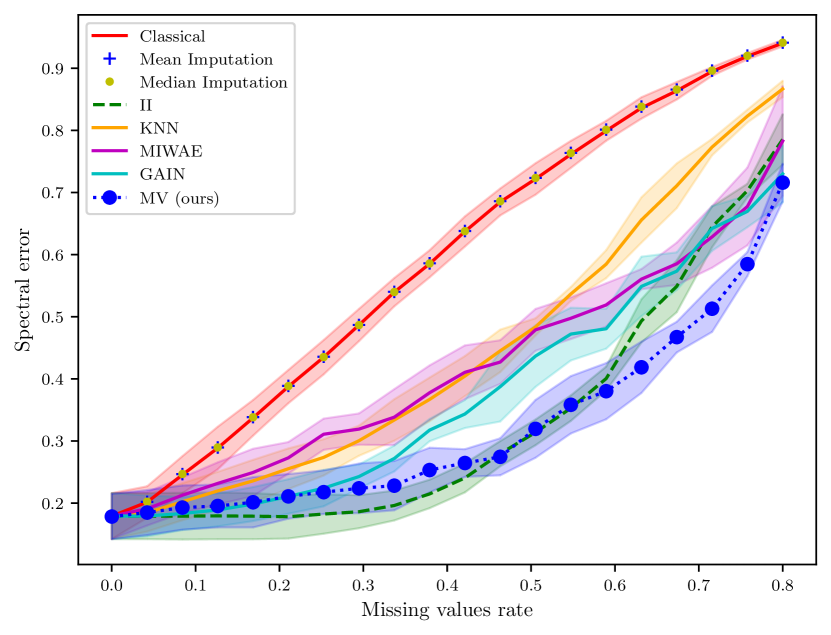
Figure 2: Estimation error on a synthetic dataset with $p=50$, $n=300$, $r\left(\Sigma\right)=5$.

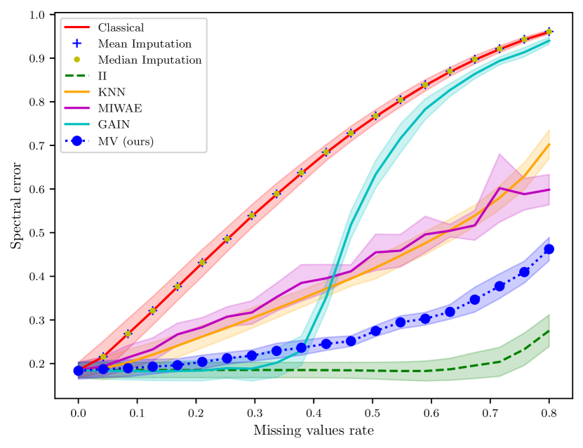
Figure 3: Estimation error on a synthetic dataset with $p=500$, $n=300$, $r\left(\Sigma\right)=5$.

5.2 Cell-wise contamination

Methods tested.

Our baselines are the empirical covariance estimator applied without care for contamination and an oracle which knows the position of every outlier, deletes them and then computes the MV bias correction procedure (6). In view of Theorems 1 and 1, this oracle procedure is the best possible in the setting of cell-wise contamination. Hence, we have a practical framework to assess the performance of any procedure designed to handle cell-wise contamination.

The SOTA methods in the cell-wise contamination setting are the DI (Detection-Inputation) method raymaekersHandlingCellwiseOutliers2020 and the TSGS method (Two Step Generalised S-estimator) agostinelliRobustEstimationMultivariate2014 . Both these methods were designed to work in the standard setting $n>p$ but cannot handle the high-dimensional setting as we already mentioned. Nevertheless, we included comparisons of our methods to them in the standard setting $n>p$. The code for DI and TSGS are from the R packages cellwise and GSE respectively.

We combine the DDC detection procedure rousseeuwDetectingDeviatingData2018 to first detect and remove outliers with several estimators developed to handle missing values. Our main estimators are DDCMV (short for Detecting Deviating Cells Missing Values), which uses first DDC and then computes the debiaised covariance estimator (6) on the filtered data, and tailMV, which detects outliers through thresholding and then uses again (6). But we also proposed to combine the DDC procedure with imputation methods KNNI, II, GAIN and MIWAE and finally compute the standard covariance estimator on the completed data. Hence we define four additional novel robust procedures which we call DDCKNN, DDCII, DDCGAIN and DDCMIWAE. To the best of our knowledge, neither the first approach combining filtering with debiasing nor the second alternative approach combining filtering with missing values imputation have never been tested to deal with cell-wise contamination. A detailed description of each method is provided in App. C.

Outlier detection and estimation error under cell-wise contamination on synthetic data.

We showed that the error of a covariance estimator under cell-wise contamination depends on the proportion of remaining outliers after a filtration. In Table 2 we investigate the filtering power of the Tail Cut and DDC methods in presence of Dirac contamination. We consider the cell-wise contamination setting (2) in the most difficult case $\varepsilon=1$ which means that an entry is either correctly observed or replaced by an outlier (in other words, the dataset does not contain any missing value). For each values of $\delta$ in a grid, the quantities $\hat{\delta}$ and $\hat{\varepsilon}$ are the proportions of true entries and remaining contaminations after filtering averaged over $20$ repetitions. The DDC based methods are particularly efficient since the proportion of Dirac contamination drops from $1-\delta$ to virtually $0$ for any $\delta\geq 0.74$. In Figures 1 and 5, we see that the performance of our method is virtually the same as the oracle OracleMV as long as the filtering procedure correctly eliminates the Dirac contaminations. As soon as the filtering procedure fails, the statistical accuracy brutally collapses and our DDC based estimators no longer do better than the usual empirical covariance. In Table 8 and Figure 5, we repeated the same experiment but with a centered Gaussian contamination. Contrarily to the Dirac contamination scenario, we see in Figure 5 that the statistical accuracy of our DDC based methods slowly degrades as the contamination rate increases but their performance remains significantly better than that of the usual empirical covariance.

Table 2: We consider contaminated data following model (2) contaminated with a Dirac contamination of high intensity with $\varepsilon=1$ and for several values of $\delta$ in a grid. For each $\delta$, we average the proportion of real data $\hat{\delta}$ and contaminated data $\hat{\varepsilon}$ after filtering over $20$ repetitions. Values are displayed in percentages ($\hat{\delta}$ must be high, $\hat{\varepsilon}$ low)). STD stands for standard deviation.

Contamination	Tail cut				DDC $99\%$				DDC $90\%$
rate ($1-\delta$)	$\hat{\delta}$	std	$\hat{\varepsilon}$	std	$\hat{\delta}$	std	$\hat{\varepsilon}$	std	$\hat{\delta}$	std	$\hat{\varepsilon}$	std
0.1 $\%$	99.6	0.023	0.000	0.000	99.1	0.029	0.000	0.000	94.8	0.054	0.00	0.00
1$\%$	98.8	0.027	0.000	0.000	98.2	0.037	0.000	0.00	94.3	0.102	0.00	0.00
5$\%$	94.9	0.013	0.000	0.000	94.6	0.018	0.000	0.000	91.8	0.060	0.00	0.000
10$\%$	90.0	0.004	0.000	0.000	89.9	0.016	0.00	0.000	88.2	0.109	0.000	0.000
20$\%$	80.0	0.000	20.0	0.000	80.0	0.003	0.017	0.035	79.4	0.035	0.009	0.022
30$\%$	70.0	0.000	30.0	0.000	70.0	0.001	3.48	2.19	69.9	0.015	2.930	2.31

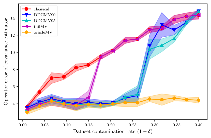
Figure 4: Estimation error as a function of the contamination rate for $n=500$, $p=400$, $\mathbf{r}(\Sigma)=5$ and Dirac contamination .

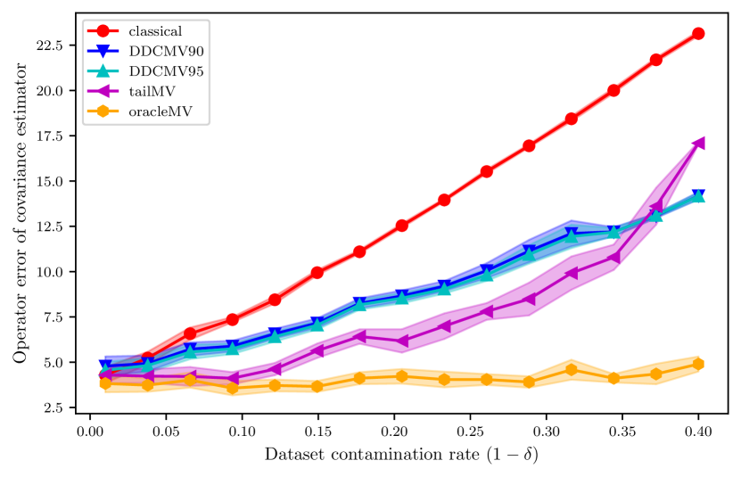
Figure 5: Estimation error as a function of the contamination rate for $n=500$, $p=400$, $\mathbf{r}(\Sigma)=5$ and Gaussian contamination .

5.3 The effect of cell-wise contamination on real-life datasets

We tested the methods on $8$ datasets from sklearn and Woolridge’s book on econometrics wooldridgeIntroductoryEconometricsModern2016 . These are low dimensional datasets (less than $20$ features) representing various medical, social and economic phenomena. We also included $2$ high-dimensional datasets. See App. B for the list of the datasets.

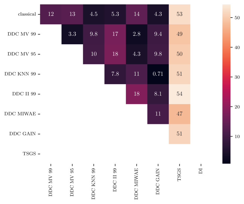
Figure 6: DI fails on ATTEND since the covariance matrix is approximately low rank. The dataset has only $8$ features and the effective rank of its covariance matrix is below $2$.

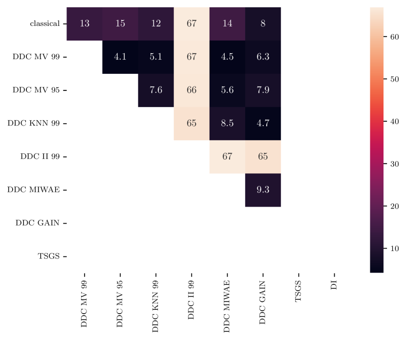
Figure 7: Woolridge’s CEOSAL dataset fails both TSGS and DI with its dimension of $13$ and effective rank of around $2.5$.

One interesting observation is that the instability of Mahalanobis distance-based algorithms is not limited to high-dimensional datasets. Even datasets with a relatively small number of features can exhibit instability. This can be seen in the performance of DI on the Attend dataset, as depicted in Figure 7, where it fails to provide accurate results. Similarly, both TSGS and DI fail to perform well on the CEOSAL2 dataset, as shown in Figure 7, despite both datasets having fewer than $15$ features.

On the Abalone dataset, once we have removed 4 obvious outliers (which are detected by both DDC and the tail procedure), all estimators reached a consensus with the non-robust classical estimator, meaning that this dataset provides a ground truth against which we can evaluate and compare the performance of robust procedures in our study. To this end, we artificially contaminate $5\%$ of the cells at random in the dataset with a Dirac contamination and compare the spectral error of the different robust estimators. As expected, TSGS and all our new procedures succeed at correcting the error, however DI becomes unstable (see Table 3). DDC MIWAE is close to SOTA TSGS for cellwise contamination and DDC II performs better. We also performed experiments on two high-dimensional datasets, where our methods return stable estimates of the covariance (DDCMV99 and DDCMV95 are within $\approx 3\%$ of each other) and farther away from the classical estimator (See Figures 9 and 9 ). Note also that DDCII’s computation time explodes and even returns out-of-memory errors due to the high computation cost of II that we already highlighted in Table 1.

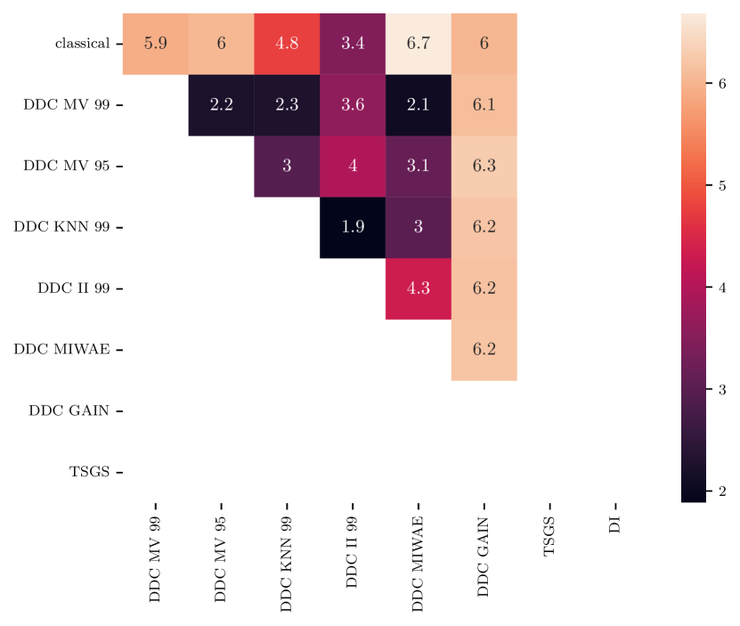
Figure 8: Relative spectral difference (in $\%$) between covariance estimators on SP500 stock returns over 2021 and 2022. On high-dimensional data, DDCII becomes inconsistent with the other procedures, maybe because II does not scale well with dimension.

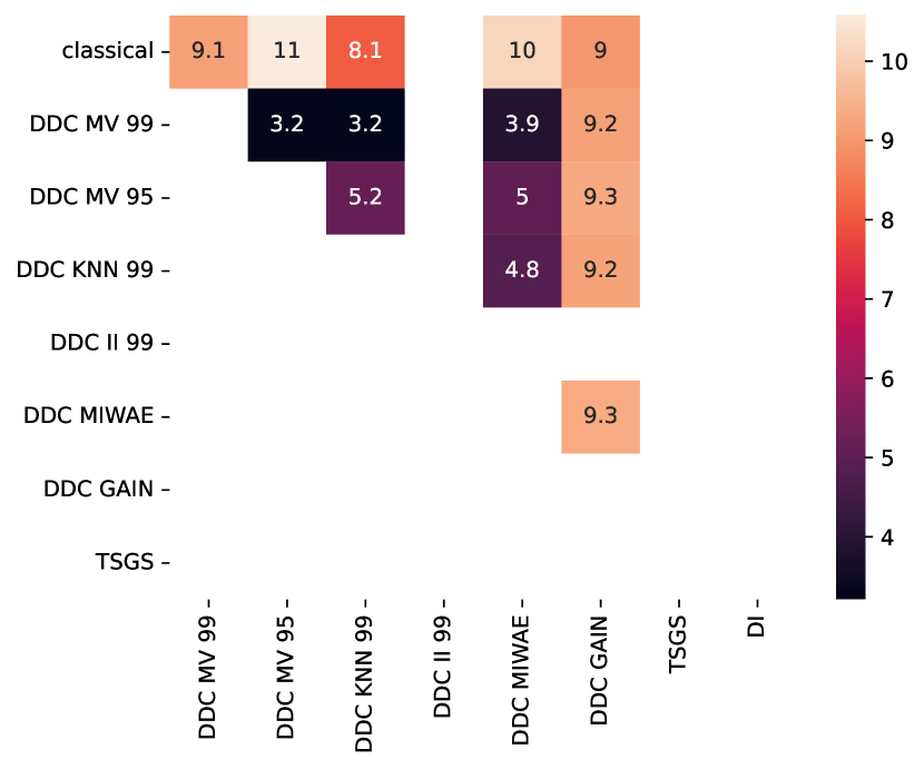
Figure 9: Relative spectral difference (in $\%$) between between covariance estimators on NASDAQ stock returns over 2021 and 2022. Here, DDCII fails due to out-of-memory errors.

Table 3: Relative spectral difference (in $\%$) between estimated covariance matrices on Abalone with $5\%$ synthetic contamination ($\delta=0.95$, $\varepsilon=1$). On the cleaned dataset, all the robust estimators are very close to the empirical covariance (relative differences $<5\%$), so we consider the empirical covariance matrix as the truth. Here the DI procedure fails probably due to numerical errors.

relative	Classical	DDCMV99	DDCMV95	DDC II	DDC KNN	DDC	DDC	TSGS	DI
error to	estimator					MIWAE	GAIN
Truth	12.8	4.12	6.81	1.70	2.06	3.46	5.06	3.06	8.85
std	0.45	0.29	0.26	0.10	0.092	0.18	0.35	0.21	1.48
Classical	-	13.1	14.3	13.0	13.0	12.9	13.1	13.4	14.9
DDCMV99	-	-	2.99	2.52	2.22	1.87	2.66	5.44	8.79
DDCMV95	-	-	-	5.27	5.03	4.04	3.71	8.28	9.99
DDC II	-	-	-	-	0.465	1.88	3.49	3.27	8.28
DDC KNN	-	-	-	-	-	1.58	3.19	3.46	8.15
DDC MIWAE	-	-	-	-	-	-	1.70	4.50	7.22
DDC GAIN	-	-	-	-	-	-	-	5.97	6.71
TSGS	-	-	-	-	-	-	-	-	6.94

6 Conclusion and future work

In this paper, we have extended theoretical guarantees on the spectral error of our covariance estimators robust to missing data to the missing at random setting. We have also derived the first theoretical guarantees in the cell-wise contamination setting. We highlighted in our numerical experimental study that in the missing value setting, our debiased estimator designed to tackle missing values without imputation offers statistical accuracy similar to the SOTA IterativeImputer for a dramatic computational gain. We also found that SOTA algorithms in the cell-wise contamination setting often fail in the standard setting $p<n$ for dataset with fast decreasing eigenvalues (resulting in approximately low rank covariance), a setting which is commonly encountered in many real life applications. This is due to the fact that these methods use matrix inversion which is unstable to small eigenvalues in the covariance structure and can even fail to return any estimate. In contrast, we showed that our strategy combining filtering with estimation procedures designed to tackle missing values produce far more stable and reliable results. In future work, we plan to improve our theoretical upper and lower bounds in the cell-wise contamination setting to fully clarify the impact of this type of contamination in covariance estimation.

Acknowledgements.

This paper is based upon work partially supported by the Chaire Business Analytic for Future Banking and EU Project ELIAS under grant agreement No. 101120237.

Appendix A presents the synthetic data generation procedure used throughout our experiments. Appendix B and in particular Table 5 list the real life datasets presented in the paper. The cell-wise contamination correction methods are shown in Appendix C, with the DDC algorithm of [34] further detailed in Appendix D for convenience. The upper bound proofs can be found in Appendix F and the lower bound proofs in Appendix G, so that similar proof techniques can be grouped together for clarity. Additional technical elements of these proofs are collected in Appendix H when we felt that they impacted the latter’s readability. Finally, we show the full results of our experiments in Appendix I.

Table 4: Notations

Symbol	Description	Symbol	Description
$X$	The random variable of interest	$\widehat{\Sigma}$	Unbiased estimator of the covariance of $X$
$Y$	The observed contaminated random variable	$\widehat{\Sigma}^{Y}$	Empirical covariance of $Y$
$p$	Dimension of the random variable	$\Lambda$	Noise covariance matrix
$n$	Number of samples	$\left\|X\right\|_{2}$	Vector $L^{2}$ norm (Euclidean norm)
$\delta$	Probability that a cell be observed correctly	$\left\|\Sigma\right\|$	Operator norm of $\Sigma$
$d$	Bernoulli random variable of probability $\delta$	$\left\|\Sigma\right\|_{F}$	Frobenius norm of $\Sigma$
$\varepsilon$	Probability that an unobserved cell be contaminated	$\left\|\Sigma\right\|_{\psi_{\alpha}}$	$\alpha$-Orlicz norm of $\Sigma$
$e$	Bernoulli random variable of probability $\varepsilon$	$\odot$	Hadamard or term by term product of matrices
$\Sigma$	True covariance matrix of $X$	$\otimes$	Outer product of vectors
$\Sigma^{Y}$	True covariance matrix of $Y$	$\mathbb{I}$	Indicator function
$\bm{r}(\Sigma)$	Effective rank of $\Sigma$	$\lesssim$	Domination with regard to an absolute constant

Appendix A Synthetic data generation

We generate synthetic datasets of $n$ realisations of a multivariate centered normal distribution. Its covariance matrix is defined as follows. We first set the eigenvalues as $\lambda_{j}=\exp\left(-j/r\right)$ for $j\in\{1,p\}$, where $r$ is the requested effective rank of the matrix. This approximation guaranties that the true effective rank is below $r+1$ for $r<<p$. Then, using the ortho-group tool from scipy.stats, we create a random orthonormal matrix $H$ and set $\Sigma=H\text{diag}(\lambda)H^{\top}$, which is symmetric and of low effective rank at most $r+1$. Finally, we divide $\Sigma$ by its largest diagonal term so that the variances of the marginals be closer to $1$.

We contaminate our synthetic datasets using a binary mask obtained by computing the realisation of $n\times p$ i.i.d. bernoulli random variables. We fill the resulting missing data with either $n$ samples of a isotropic gaussian of covariance $\sigma I_{p}$, where $\sigma$ is the strength of the contamination (which we call the Gaussian contamination) or a $n\times p$ array of value $\pm\sigma$ (which we call the Dirac contamination). Let $\xi$ be a random vector following one of those two contaminations, the data we feed all algorithms is then $Y=\text{mask}\odot X+(1-\text{mask})\odot\xi$.

Appendix B Real life data set

For our real data experiments, we removed any categorical variable from the datasets since this work focuses on covariance estimation.We also applied a log transform to skewed variables to ensure that they are sub-Gaussian. The list of datasets can be found in Table 5. Finally, the Abalone dataset contains four obvious outliers that we removed in our experiments (although they were easily detected by both DDC and the thresholding procedure) in order to obtain a perfect dataset (no missing values, no contaminations) allowing us to compute the ground truth covariance. We have then injected missing values and cell-wise contaminations in this dataset and compared our robust procedures to the ground truth. We also note that the three UCI datasets were downloaded from sklearn.

Table 5: Datasets used in our real-life experiments. $p$ and $n$ are indicated after dropping categorical features and obvious sample-wise outliers.

Name	Source	$p$	$n$	$r\left(\Sigma\right)$	Description
Abalone	UCI	7	4173	1.0	Caracteristics of abalone specimens
Breast Cancer	UCI	13	178	2.3	Data on cell nuclei
Wine	UCI	30	69	2.8	Chemical data on wine varieties
Cameras	R	11	1038	2.7	Camera caracteristics over different models
Attend	[46]	8	680	2.0	Class attendance
Barium	[46]	11	131	2.4	Barium exports
CEOSAL2	[46]	13	177	2.5	Firm accountancy data
INTDEF	[46]	12	49	2.2	USA deficit
SP 500	yfinance	496	502	2.7	Returns of SP 500 companies in 2021/2022
NASDAQ	yfinance	1442	502	4.0	Returns of NASDAQ companies in 2021/2022

Appendix C Methods compared in the cell-wise contamination setting

C.1 Baseline methods

Classical

denotes the empirical covariance estimator applied without care for contamination. We expect all other methods to perform better than it.

oracleMV

is an oracle that knows which cells are contaminated. This method shows the performance of our corrected estimator in the case of a perfect outlier detection algorithm, hence providing an idea of the optimal precision attainable with regard to the available information.

C.2 Our methods

tailMV

or tail Missing Values, is an estimator built by deleting extreme values in the dataset. It is actually one of the intermediary steps of DDC and we wanted to test how efficient it was on its own. We use the robust Huber estimator of the python package Statsmodel.robust [12] to compute the standard deviation of each marginal and eliminate any cell with value above $3$ times these estimates.

DDCMV

short for Detecting Deviating Cells Missing Values, is an estimator built using the DDC detection procedure of [32], where detected outliers are removed and considered as missing values. A detailed description of DDC is provided in appendix D. We then apply our corrected covariance estimator. We will add to the name of the method the quantile at which we consider a data as an outlier (DDCMV99 uses the 99-percentile of $\chi^{2}_{1}$ for instance). When nothing is mentioned, assume that DDCMV99 is used. In our experiments, we use the R implementation found in the package cellWise, whose results are then sent to a python script for formatting.

DDCKNN

detects outliers with the DDC procedure, removes them and imputes the missing values using the k-nearest neighbour procedure of [39] as implemented in sklearn under the name KNNImputer.

DDCII

also detects and removes outliers with the DDC procedure, then imputes the missing values using sklearn’s Iterative Imputer class.

DDCGAIN

is the combination of the DDC algorithm for outlier detection followed by the GAIN deep imputation method of [47].

DDCMIWAE

is the combination of the DDC algorithm for outlier detection followed by the MIWAE deep imputation method of [28].

C.3 SOTA methods for cell-wise contamination

DI

or Detection Imputation [33] Is an iterative algorithm made of two alternating steps inspired by the Expectation Maximisation (EM) algorithm. The first detects outliers with regard to a previously estimated covariance matrix, then the second computes a new covariance matrix having removed the previously detected outliers using the M step of EM, but with bias correction. This new matrix is then the basis for the next detection step and so on. The authors found their algorithm to have a $O(Tnp^{3})$ complexity, with $T$ the number of iterations, and make the assumption that the covariance matrix is of full rank to perform matrix inversion, both facts that make it difficult to use in high dimensions.

TSGS

or Two Steps Generalised S-estimator [2] and [24] is also based on a two step process of detection then correction. Detection is based on the same DDC procedure while the estimation phase is based on the Generalised S-estimator of [6]. S-estimators are based on the Mahalonobis distance and thus require the true covariance matrix to be invertible. This may lead to numerically instability in our approximately low rank setting. However, if the matrix is of full rank, the generalised version of these estimators are proven to be consistent in the Missing Completely At Random setting.

Appendix D The Detecting Deviating Cells algorithm

This section is entirely based on [34], whose algorithm we describe here for convenience. DDC (Detecting Deviating Cells) is a 7 steps algorithm. In the following, let $(X_{i}^{j})_{i\in[n],j\in[p]}$ be our dataset of $n$ samples from data with dimension $p$.

Step 1: standardisation

We start by assuming that the $X_{i}$ follow a normal distribution and we set

$$Z_{i}^{j}=\frac{X_{i}^{j}-\mu_{X}^{j}}{\sigma_{X}^{j}}$$

with $\mu_{X}^{j}$ being the empirical mean of marginal $j$, and $\sigma_{X}^{j}$ its standard deviation.

Step 2: cutoff

DDC sets to NA all values of $Z_{i}^{j}$ if

$$|Z_{i}^{j}|\geq\sqrt{\chi^{2}_{1,p}}$$

with $\chi^{2}_{1,p}$ the $p^{\text{th}}$ centile of a $\chi^{2}_{1}$ distribution, where $p=99\%$ by default.

Step 3: bivariate relationship

The algorithm then computes the correlation between each couple of marginals. If $|\rho_{i}(Z^{j},Z^{k})|\leq 0.5$; set $b_{jk}=0$. Otherwise,

$$b_{jk}=\text{slope}(Z^{j}|Z^{k})$$

with $\text{slope}(x|y)$ the robust slope in the linear regression of $x$ using $y$.

Step 4: comparison

Then DDC tries to predict the expected values of each $Z_{i}^{j}$ according to a weighted mean of the values of the other marginals, using the previously computed correlations as weights.

$$\hat{Z}_{i}^{j}=G\left(\{b_{jk}Z_{i}^{k},k\in[p],k\neq j\}\right)$$

with $G$ the weighted mean using $\rho(Z^{j},Z^{h})$ as weights.

Step 5: deshrinkage

DDC adjusts the mean to account for shrinkage.

$$\begin{split}a_{j}&=\text{slope}(Z_{i}^{j}|\hat{Z}_{i}^{j})\\ Z^{j\star}_{i}&=a_{j}\hat{Z}_{i}^{j}\end{split}$$

Step 6: residual computation

Then, one can take the residuals:

$$r_{i}^{j}=\frac{Z_{i}^{j}-\hat{Z}_{i}^{j}}{\mu_{Z^{j}-\hat{Z}^{j}}}$$

Step 7: destandardisation

Finally, DDC returns the data to its actual location and scale. The residuals can then be tested using a $\chi^{2}_{1}$ law to determine whether or not they are outliers.

Appendix E Missing at Random experiment

To assess our estimator (8) in the heterogeneous missingness setting, we replicated the MAR experiment of [28, Annex 3]. In this experiment, the data is missing with a different probability for each feature. These probabilities are fixed prior to the experiment and depend on the data, although the bernoulli random variables are still independent to the data. Just as in [28], the probability $\delta_{j}$ that an $X^{j}$ is observed depends on the first 15 samples and:

$$\delta_{j}=1-\text{sigmoid}\left(\frac{1}{15}\sum_{j=1}^{15}x_{j}\right)$$ (13)

We compared our debiasing estimator (8) to the traditional KNNimputer, IterativeImputer and the recent imputation methods GAIN and MIWAE which are expected to perform better in this setting. On the Abalone dataset (Table 7), MV is the most accurate for the operator norm and MIWAE and GAIN are far behind and performs worse than IterativeImputer or KNNimputer. The Breast Cancer data was used both in [28, 47]. We used the colab code provided by [28] to implement MIWAE method. For GAIN we use the defaults parameters as in the HyperImpute library. We see in Table 7 that GAIN is the second best method behind MV and is better than IterativeImputer. We also note that, in all our experiments, the computation times were far longer for GAIN and MIWAE than for our debiasing scheme MV.

Table 6: Abalone

Method	mean error	std
classical	$59.33$	$0.58$
MV	$\bm{1.87}$	$0.57$
II	$4.28$	$1.44$
KNN	$4.55$	$1.31$
GAIN	$16.5$	$2.09$
MIWAE	$8.60$	$0.62$

Table 7: Breast cancer

Method	mean error	std
classical	$88.63$	$0.46$
MV	$\bm{21.74}$	$3.00$
II	$69.79$	$2.53$
KNN	$61.97$	$10.04$
GAIN	$37.46$	$5.78$
MIWAE	$87.96$	$0.43$

Appendix F Proofs of upper bounds

F.1 Tools and definitions

F.1.1 Basic properties of random vectors

We recall the definition and some basic properties of sub-exponential random vectors.

Definition 1.

For any $\alpha\geq 1$, the $\psi_{\alpha}$-norms of a real-valued zero mean random variable $V$ are defined as:

$$\left\|V\right\|_{\psi_{\alpha}}=\inf\{u>0,\mathbb{E}\exp\left(|V|^{\alpha}/u^{\alpha}\right)\leq 2\}$$

We say that a random variable $V$ with values in $\mathbb{R}$ is sub-exponential if $\left\|V\right\|_{\psi_{\alpha}}<\infty$ for some $\alpha\geq 1$. If $\alpha=2$, we say that $V$ is sub-Gaussian.

Lemma 2 (Lemma 5.14 in [43]).

If a real-valued random variable $V$ is sub-Gaussian, then $V^{2}$ is sub-exponential. Indeed, we have:

$$\left\|V\right\|_{\psi_{2}}^{2}\leq\left\|V^{2}\right\|_{\psi_{1}}\leq 2\left\|V\right\|_{\psi_{2}}^{2}$$

.

Definition 2.

The $\psi_{\alpha}$-norms of a random vector $X$ are defined as:

$$\left\|X\right\|_{\psi_{\alpha}}=\sup_{x\in\mathbb{R}^{p},|x|_{2}=1}\left\|\langle X,x\rangle\right\|_{\psi_{\alpha}},\qquad\alpha\geq 1$$

We will use the following definition of sub-Gaussian vectors that can be found in [20].

Definition 3.

A random vector $X\in\mathbb{R}^{p}$ is sub-Gaussian if and only if $\forall x\in\mathbb{R}^{p}$, $\left\|\langle X,x\rangle\right\|_{\psi_{2}}\lesssim\left\|\langle X,x\rangle\right\|_{L^{2}}$.

We recall a version of Bernstein’s inequality (see corollary 5.17 in [43]):

Proposition 1.

Let $Z_{1},\dots Z_{n}$ be independent sub-exponential zero mean real-valued random variables. Set $K=\max_{i}\left\|Z_{i}\right\|_{\psi_{1}}$. Then, for $t>0$, with probability at least $1-e^{-t}$:

$$\left|n^{-1}\sum_{i=1}^{n}Z_{i}\right|\leq CK\left(\sqrt{\frac{t}{n}}\lor\frac{t}{n}\right)$$ (14)

where $C$ is an absolute constant.

F.2 Proofs of upper bounds in the setting of heterogeneous missingness

We denote by $\text{off}(A)$ the matrix obtained by putting to $0$ the diagonal entries of matrix $A$.

Following [26], we first note that

$$\left\|\widehat{\Sigma}-\Sigma\right\|\leq\left\|\Delta_{\text{inv}}\odot\text{off}\left(\widehat{\Sigma}^{Y}-\Sigma^{Y}\right)\right\|+\left\|\text{diag}(\delta_{\text{inv}})\odot\left(\widehat{\Sigma}^{Y}-\Sigma^{Y}\right)\right\|.$$ (15)

Hence, in view of [16, Theorem 3.1.d, page 95], we have that

$$\left\|\widehat{\Sigma}-\Sigma\right\|\leq\text{\@text@baccent{$\delta$}}^{-2}\left\|\text{off}\left(\widehat{\Sigma}^{Y}-\Sigma^{Y}\right)\right\|+\text{\@text@baccent{$\delta$}}^{-1}\left\|\text{diag}(\widehat{\Sigma}^{Y}-\Sigma^{Y})\right\|.$$ (16)

We now extend several arguments in [26, 18] developed in the MCAR setting (same observation rate $\delta$ for all the features) to the heterogeneous missingness setting where each feature $j$ has possibly a different observation rate $\delta_{j}$ from the others features.

Lemma 3.

Let $X\in\mathbb{R}^{p}$ be a random vector admitting covariance $\Sigma$. Define $Y^{(j)}=d^{(j)}X^{(j)}$ for all $j\in[p]$, where the $d^{(j)}$ are independent Bernoulli random variables with $\mathbb{E}d^{(j)}=\delta_{j}$ and $\bar{\delta}=\max_{j}\delta_{j}$. We have

$$\left\|\mathbb{E}\left[(YY^{\top}-\text{diag}(YY^{\top}))^{2}\right]\right\|\lesssim\bar{\delta}^{2}\text{tr}\left(\Sigma\right)\left\|\Sigma\right\|,$$

and

$$\left\|\mathbb{E}\left[(\text{diag}(YY^{\top}))^{2}\right]\right\|\lesssim\bar{\delta}\left\|\Sigma\right\|^{2}.$$

Proof.

Let us first look at $\mathbb{E}\left[(YY^{\top}-\text{diag}(YY^{\top}))^{2}\right]$. We define $\sqrt{\delta}=(\sqrt{\delta_{1}}\dots,\sqrt{\delta_{p}})^{\top}$. We also denote by $\mathbb{E}_{d}$ the conditional expectation with respect to $d$ given $X$. We compute the following representation:

$$\begin{split}\mathbb{E}_{d}\text{off}\left(YY^{\top}\right)^{2}&=\mathbb{E}_{d}\text{off}\left((d\otimes d)\odot(X\otimes X)\right)^{2}\\ &=\left\|\sqrt{\delta}\odot X\right\|_{2}^{2}\text{off}\left((\delta\otimes\delta)\odot(X\otimes X)\right)\\ &\hskip 14.22636pt-\left(\text{diag}\left((\sqrt{\delta}\otimes\sqrt{\delta})\odot(X\otimes X)\right)\right)\left(\text{off}\left((\delta\otimes\delta)\odot(X\otimes X)\right)\right)\\ &\hskip 14.22636pt-\left(\text{off}\left((\delta\otimes\delta)\odot(X\otimes X)\right)\right)\left(\text{diag}\left((\sqrt{\delta}\otimes\sqrt{\delta})\odot(X\otimes X)\right)\right).\end{split}$$

Let us name the following matrices:

• $A=\left((\delta\otimes\delta)\odot(X\otimes X)\right)$
  

• $B=((\sqrt{\delta}\otimes\sqrt{\delta})\odot(X\otimes X))$
  

• $C=\text{off}\left((\delta\otimes\delta)\odot(X\otimes X)\right)$
  

• $D=\text{diag}\left((\sqrt{\delta}\otimes\sqrt{\delta})\odot(X\otimes X)\right)$

We note first that $\text{off}(A)=A-\text{diag}(A)\leq A$ since $\text{diag}(A)$ is positive semi-definite. Here this inequality is to be understood in the matrix sense (Let $A$ and $B$ be $p\times p$ symmetric matrices. We say that $A\leq B$ if for any $u\in\mathbb{R}^{p}$, $u^{\top}Au\leq u^{\top}Bu$).

Notice also that $-CD-DC\leq(C-D)^{2}$. Finally, we have that $C-D=A-\text{diag}(A+B)$. Hence:

$$\begin{split}\mathbb{E}_{X}\text{off}\left(YY^{\top}\right)^{2}&\leq\left\|\sqrt{d}\odot X\right\|_{2}^{2}A+\left(A-\text{diag}(A+B)\right)^{2}\\ &\leq\left\|\sqrt{\delta}\odot X\right\|_{2}^{2}A+2\left(\text{diag}(A+B)\right)^{2}+2A^{2}.\end{split}$$ (17)

Let us now compute the expectations according to $X$. Following [26], we find that:

$$\mathbb{E}A^{2}\leq\text{tr}\left((\delta\otimes\delta)\odot\Sigma\right)\left((\delta\otimes\delta)\odot\Sigma\right)\leq\bar{\delta}^{2}\text{tr}\left(\Sigma\right)\left[(\delta\otimes\delta)\odot\Sigma\right].$$ (18)

By elementary computations

$$\left\|(\delta\otimes\delta)\odot\Sigma\right\|=\max_{u\,:\,\left\|u\right\|=1}\{\langle(\delta\otimes\delta)\odot\Sigma u,u\rangle\}=\max_{u\,:\,\left\|u\right\|=1}\{\langle\Sigma(\delta\odot u),(\delta\odot u)\rangle\}.$$

Hence $\left\|(\delta\otimes\delta)\odot\Sigma\right\|\leq\bar{\delta}^{2}\left\|\Sigma\right\|$ and

$$\left\|\mathbb{E}A^{2}\right\|\lesssim\bar{\delta}^{4}\text{tr}\left(\Sigma\right)\left\|\Sigma\right\|.$$ (19)

Next, we tackle the diagonal matrix. By the equivalence of the moment of sub-Gaussian distributions we have that $\mathbb{E}[(X^{(j)})^{4}]\lesssim\Sigma_{jj}^{2}\leq\left\|\Sigma\right\|$. Thus we get that:

$$\begin{split}\left\|\mathbb{E}\left(\text{diag}(A)\right)^{2}\right\|&=\left\|\mathbb{E}\text{diag}\left(\delta_{1}^{4}\mathbb{E}[(X^{(1)})^{4}],\ldots,\delta_{p}^{4}\mathbb{E}[(X^{(p)})^{4}]\right)\right\|\lesssim\bar{\delta}^{4}\left\|\Sigma\right\|^{2}.\end{split}$$

Finally, let us compute $\left\|\mathbb{E}\left[\left\|\sqrt{d}\odot X\right\|_{2}^{2}A\right]\right\|$. For any $u\in\mathbb{R}^{p}$ such that $|u|_{2}=1$, we have by Cauchy-Schwartz

$$\begin{split}\mathbb{E}\left[\left\|\sqrt{\delta}\odot X\right\|_{2}^{2}\langle Au,u\rangle\right]&=\mathbb{E}\left[\left\|\sqrt{\delta}\odot X\right\|_{2}^{2}\langle X\odot\delta,u\rangle^{2}\right]\\ &\leq\left(\mathbb{E}\left[\left\|\sqrt{\delta}\odot X\right\|_{2}^{4}\right]\mathbb{E}\left[\langle X\odot\delta,u\rangle^{4}\right]\right)^{\frac{1}{2}}.\end{split}$$

Looking at the first expectation:

$$\begin{split}\mathbb{E}\left[\left\|\sqrt{\delta}\odot X\right\|_{2}^{4}\right]&=\mathbb{E}\left(\sum_{j\in[p]}\delta_{j}(X^{(j)})^{2}\right)^{2}\leq\bar{\delta}^{2}\mathbb{E}\left(\sum_{j\in[p]}(X^{(j)})^{2}\right)^{2}=\bar{\delta}^{2}\mathbb{E}\left\|X\right\|_{2}^{4}.\end{split}$$

Exploiting the sub-Gaussianity of $X$, it was proved in [26] that

$$\mathbb{E}\left\|X\right\|_{2}^{4}\lesssim(\mathrm{tr}(\Sigma))^{2}.$$

We study now the term $\mathbb{E}\langle X\odot\delta,u\rangle^{4}$. Again by sub-Gaussianity of $X$, we have equivalence of the moments. That is for any unit vector $u\in\mathbb{R}^{p}$

$$\begin{split}\mathbb{E}\langle X\odot\delta,u\rangle^{4}&=\mathbb{E}\langle X,u\odot\delta\rangle^{4}\\ &\lesssim\left(\mathbb{E}\langle X,u\odot\delta\rangle^{2}\right)^{2}=\langle\Sigma u\odot\delta,u\odot\delta\rangle^{2}\leq\left\|\Sigma\right\|^{2}|u\odot\delta|_{2}^{4}\leq\bar{\delta}^{4}\left\|\Sigma\right\|^{2}.\end{split}$$

Combining the last four displays, we obtain that

$$\left\|\mathbb{E}\left[\left\|\sqrt{d}\odot X\right\|_{2}^{2}A\right]\right\|\lesssim\bar{\delta}^{3}\mathrm{tr}(\Sigma)\left\|\Sigma\right\|.$$ (20)

The second inequality of the lemma follows from a similar and actually simpler argument. We have

$$\begin{split}\left\|\mathbb{E}\left[\text{diag}(YY^{\top})^{2}\right]\right\|=\max_{j}\mathbb{E}\left[d^{(j)}(X^{(j)})^{4}\right]\lesssim\bar{\delta}\left\|\Sigma\right\|^{2},\end{split}$$

where we have used again the sub-Gaussianity of the random vector $X$ and the fact that $\Sigma_{jj}\leq\left\|\Sigma\right\|$ for any $j\in[p]$. ∎

Lemma 4.

Under the same assumptions as the previous lemma, for any $u\in\mathbb{R}^{p}$ such that $|u|_{2}=1$,

$$\mathbb{E}\left(u^{\top}(YY^{\top}-\text{diag}(YY^{\top}))u\right)^{2}\lesssim\bar{\delta}^{2}\left\|\Sigma\right\|^{2},$$

and

$$\mathbb{E}\left(u^{\top}\,\text{diag}(YY^{\top})u\right)^{2}\lesssim\bar{\delta}\left\|\Sigma\right\|.$$

Proof.

Let us consider two vectors $\bm{a}$ and $\bm{b}$ of $\mathbb{R}^{p}$. First, let us demonstrate the first assertion. By using $\mathbb{E}Z^{2}=\mathbb{E}(Z-\mathbb{E}Z)^{2}+(\mathbb{E}Z)^{2}$ :

$$\begin{split}\mathbb{E}\left(\sum_{i\neq j}d^{(i)}d^{(j)}a_{i}b_{j}\right)=\mathbb{E}\left(\sum_{i\neq j}(d^{(i)}-\delta_{i})(d^{(j)}-\delta_{j})a_{i}b_{j}\right)+\left(\sum_{i\neq j}\delta_{i}\delta_{j}a_{i}b_{j}\right).\end{split}$$

Looking at the first term, we use the decoupling principle of [44, Theorem 6.1.1] to create $d^{\prime}$ an independent copy of $d$ with same law such that:

$$\begin{split}\mathbb{E}\left(\sum_{i\neq j}(d^{(i)}-\delta_{i})(d^{(j)}-\delta_{j})a_{i}b_{j}\right)&\leq 16\mathbb{E}\left(\sum_{i\neq j}(d^{(i)}-\delta_{i})(d^{\prime(j)}-\delta_{j})a_{i}b_{j}\right)\\ &\leq 16\sum_{i\neq j}\sum_{k\,eql}\mathbb{E}(d^{(i)}-\delta_{i})(d^{\prime(j)}-\delta_{j})(d^{(k)}-\delta_{i})(d^{\prime(l)}-\delta_{j})a_{i}b_{j}a_{k}b_{l}.\end{split}$$

Here all the terms except $k=i$ and $l=j$ are equal to zero. We have that for all $j$, $\mathbb{E}(d^{(i)}-\delta_{j})^{2}=\delta_{j}(1-\delta_{j})\leq\bar{\delta}$ thus:

$$\begin{split}\mathbb{E}\left(\sum_{i\neq j}(d^{(i)}-\delta_{i})(d^{(j)}-\delta_{j})a_{i}b_{j}\right)&\leq 16\sum_{i\neq j}a_{i}^{2}b_{j}^{2}\delta_{i}(1-\delta_{i})\delta_{j}(1-\delta_{j})\\ &16\sum_{i\neq j}a_{i}^{2}b_{j}^{2}\bar{\delta}^{2}\leq 16\bar{\delta}^{2}|\bm{a}|_{2}^{2}|\bm{b}|_{2}^{2}.\end{split}$$

The second term can be bounded using $(x+y)^{2}\leq 2x^{2}+2y^{2}$ and Cauchy-Schwarz:

$$\begin{split}\left(\sum_{i\neq j}\delta_{i}\delta_{j}a_{i}b_{j}\right)&\leq 2\left(\sum_{i}\delta_{i}^{2}a_{i}b_{i}\right)^{2}+2\left(\sum_{i,j}\delta_{i}\delta_{j}a_{i}b_{j}\right)^{2}\\ &\leq 2\left(\sum_{i}\delta_{i}^{2}|a_{i}b_{i}|\right)^{2}+2\left(\sum_{i,j}\delta_{i}\delta_{j}|a_{i}b_{j}|\right)^{2}\\ &\leq 2\bar{\delta}^{2}\left(\sum_{i}|a_{i}b_{i}|\right)^{2}+2\bar{\delta}^{4}\left(\sum_{i,j}|a_{i}b_{j}|\right)^{2}.\end{split}$$

The rest of the proof follows the same arguments to those in the proof of [18, Lemma 4.4].

Regarding the second assertion, it is immediate to see that:

$$\begin{split}\mathbb{E}\left(u^{\top}\text{diag}(YY^{\top})u\right)^{2}&=\mathbb{E}\left(\sum_{j}d^{(j)}u_{j}^{2}X^{(j)^{2}}\right)^{2}\\ &=\sum_{j}\delta_{j}u_{j}^{4}\mathbb{E}(X^{(j)})^{4}+\sum_{i\neq j}\delta_{i}\delta_{j}u_{i}^{2}\mathbb{E}\left[(X^{(i)})^{2}(X^{(j)})^{2}\right]u_{j}^{2}\\ &\leq\bar{\delta}^{2}\left\|\Sigma\right\|^{2}+(\bar{\delta}-\bar{\delta}^{2})\sum_{j}u_{j}^{4}\left\|\Sigma\right\|^{2}\lesssim\bar{\delta}\left\|\Sigma\right\|^{2}.\end{split}$$

∎

We can now apply the Bernstein inequality [18, Proposition 4.1] to each term in the right-hand-side of (16).

F.3 Proof of the upper bounds in the contaminated case

Proof of Theorem 4.

First, observe that:

$$\begin{split}\left\|\widehat{\Sigma}-\Sigma\right\|&\leq 2*\delta^{-2}\left\|\widehat{\Sigma}^{Y}-\Sigma^{Y}\right\|+\frac{\varepsilon(1-\delta)}{\delta}\left\|\Lambda\right\|\end{split}$$ (21)

Thus we need to control the error on the observed covariance matrix. Here the error can decomposed as follows:

$$\left\|\widehat{\Sigma}^{Y}-\Sigma^{Y}\right\|\leq\left\|\widehat{\Sigma}^{\delta}-\Sigma^{\delta}\right\|+\left\|\widehat{\Lambda}^{\varepsilon}-\Lambda^{\varepsilon}\right\|+\left\|\widehat{\Sigma}^{X\xi\delta\varepsilon}\right\|.$$ (22)

where the three empirical matrices are

1. $\widehat{\Sigma}^{\delta}=n^{-1}\sum_{i=1}^{n}(d_{i}\otimes d_{i})\odot(X_{i}\otimes X_{i})$, the empirical covariance matrix of the $d_{i}\odot X_{i}$ and $\Sigma^{\delta}=\mathbb{E}\left[\widehat{\Sigma}^{\delta}\right]$;

2. $\widehat{\Lambda}^{\varepsilon}=n^{-1}\sum_{i=1}^{n}\left([(1-d_{i})\odot e_{i}]\otimes[(1-d_{i})\odot e_{i}]\right)\odot(\xi_{i}\otimes\xi_{i})$, the empirical covariance of the $(1-d_{i})\odot e_{i}\odot\xi_{i}$ is such that $\Lambda^{\varepsilon}=\mathbb{E}\widehat{\Lambda}^{\varepsilon}=\varepsilon(1-\delta)\Lambda$;

3. $\widehat{\Sigma}^{X,\xi,\delta,\varepsilon}=n^{-1}\sum_{i=1}^{n}\left(d_{i}\otimes[(1-d_{i})\odot e_{i}]\right)\odot(X_{i}\otimes\xi_{i})+([(1-d_{i})\odot e_{i}]\otimes d_{i})\odot(\xi_{i}\otimes X_{i})$ is the empirical covariance between the $d_{i}\odot X_{i}$ and the $(1-d_{i})\odot e_{i}\odot\xi_{i}$ and has a null diagonal and also a null expectation.

Using [18], we get that there exists an absolute constant $C>0$ such that, with probability at least $1-e^{-t}$,

$$\left\|\widehat{\Sigma}^{\delta}-\Sigma^{\delta}\right\|\leq C\delta\left\|\Sigma\right\|\left(\sqrt{\frac{\bm{r}(\Sigma)\log\bm{r}(\Sigma)}{n}}\lor\sqrt{\frac{t}{n}}\lor\frac{\bm{r}(\Sigma)(t+\log\bm{r}(\Sigma))}{\delta n}\log(n)\right)$$ (23)

To tackle the second term, we will use a standard argument for isotropic sub-Gaussian random vectors (see for instance the proof of Theorem 5.39 in [43]) combining a vector Bernstein inequality [43, Corollary 5.17] with an union bound. Hence we obtain with probability at least $1-e^{-t}$

$$\left\|\widehat{\Lambda}^{\varepsilon}-\mathbb{E}\widehat{\Lambda}^{\varepsilon}\right\|\lesssim(1-\delta)\varepsilon\sigma_{\xi}^{2}\left\|(1-d)\odot e\odot\xi\right\|_{\psi_{1}}\left(\sqrt{\frac{p}{n}}\vee\frac{p}{n}\vee\sqrt{\frac{t}{n}}\vee\frac{t}{n}\right).$$ (24)

Set $d^{\prime}=(1-d)\odot e$ and $\varepsilon^{\prime}=(1-\delta)\varepsilon$. We note that $d^{\prime}_{j}\sim B(\varepsilon^{\prime})$ for any $j\in[p]$. Using the properties of the Orlicz norm, we easily get that $\left\|d^{\prime}\odot\xi\right\|_{\psi_{1}}\leq\left\|d^{\prime}\right\|_{\psi_{2}}\left\|\xi\right\|_{\psi_{2}}$. Next, by triangular inequality, we note that $\left\|d^{\prime}\right\|_{\psi_{2}}\leq\left\|d^{\prime}-\delta\mathds{1}\right\|_{\psi_{2}}+\left\|\varepsilon^{\prime}\mathds{1}\right\|_{\psi_{2}}\lesssim\left\|d-\varepsilon^{\prime}\mathds{1}\right\|_{\psi_{2}}+\varepsilon^{\prime}$. Theorem 1.1 in [36] guarantees that $\left\|d^{\prime}-\varepsilon^{\prime}\mathds{1}\right\|_{\psi_{2}}\lesssim\sqrt{\frac{1-2\varepsilon^{\prime}}{4\log((1-\varepsilon^{\prime})/\varepsilon^{\prime})}}\lesssim\frac{1}{\sqrt{|\log\varepsilon^{\prime}|}}$ for any $\varepsilon^{\prime}<1/4$. Since $\varepsilon^{\prime}\log\varepsilon^{\prime}\rightarrow 0$ as $\varepsilon^{\prime}\rightarrow 0+$, we obtain that $\left\|d^{\prime}\right\|_{\psi_{2}}\lesssim\frac{1}{\sqrt{|\log\varepsilon^{\prime}|}}$.

Hence the previous display becomes

$$\left\|\widehat{\Lambda}^{\varepsilon}-(1-\delta)\varepsilon\sigma_{\xi}^{2}I_{p}\right\|\lesssim\frac{(1-\delta)\varepsilon}{\sqrt{|\log((1-\delta)\varepsilon)}|}\sigma_{\xi}^{2}\left(\sqrt{\frac{p}{n}}\vee\frac{p}{n}\vee\sqrt{\frac{t}{n}}\vee\frac{t}{n}\right).$$ (25)

Now we need to control the norm of

$$\widehat{\Sigma}^{X,\xi,\delta,\varepsilon}=n^{-1}\sum_{i=1}^{n}\left(d_{i}\otimes[(1-d_{i})\odot e_{i}]\right)\odot(X_{i}\otimes\xi_{i})+([(1-d_{i})\odot e_{i}]\otimes d_{i})\odot(\xi_{i}\otimes X_{i}).$$

To this end, we apply again the noncommutative Bernstein inequality of [18, Proposition 4.1]. Note that this result was stated for Hermitian matrices, but the result can be easily extended to arbitrary matrices by applying the self-adjoint dilation trick (See for instance [38] for more details).

In what follows, for any $i\in[n]$, we set

$$Z_{i}:=\left(d_{i}\otimes[(1-d_{i})\odot e_{i}]\right)\odot(X_{i}\otimes\xi_{i})+([(1-d_{i})\odot e_{i}]\otimes d_{i})\odot(\xi_{i}\otimes X_{i}).$$

For the sake of simplicity, we will write $Z$ without any index $i$ to designate any of the $Z_{i}$’s. Notice that $Z$ is symmetric by construction but has no diagonal term.

Lemma 5.

Under the assumptions of Theorem 4, we have

$$\left\|\mathbb{E}Z^{\top}Z\right\|\leq\delta^{2}(1-\delta)\varepsilon(p-2)\sigma_{\xi}^{2}\left[2\left\|\Sigma\right\|+\sigma_{\xi}^{2}\right]+\delta(1-\delta)\varepsilon\sigma_{\xi}^{4}\left(\left|\mathrm{tr}(\Sigma)-\delta(p-2)\right|+\left\|\Sigma\right\|\right).$$

Proof.

We first compute the matrix product $Z^{\top}Z$. For any $k,l\in[p]$

$$\begin{split}\left(Z^{\top}Z\right)_{kl}=&\sum_{j=1}^{p}Z_{kj}Z_{jl}\\ =&\sum_{j=1}^{p}\left(\underbrace{d^{(k)}\left(1-d^{(j)}\right)e^{(j)}X^{(k)}\xi^{(j)}}_{(i)}+\underbrace{d^{(j)}\left(1-d^{(k)}\right)e^{(k)}X^{(j)}\xi^{(k)}}_{(ii)}\right)\\ &\qquad\times\left(\underbrace{d^{(j)}\left(1-d^{(l)}\right)e^{(l)}X^{(j)}\xi^{(l)}}_{(iii)}+\underbrace{d^{(l)}\left(1-d^{(j)}\right)e^{(j)}X^{(l)}\xi^{(j)}}_{(iv)}\right)\end{split}$$ (26)

Let us call $i$ and $ii$ the two terms inside the first factor and $iii$ and $iv$ the two terms in the second factor. Observe that most terms simplify when taking the expectation:

• $\bm{(i)}$ times $\bm{(iii)}$: is always zero. Indeed, if $j\neq l$ then by independence of $\xi^{(j)}$ and $\xi^{(l)}$; otherwise $d^{(l)}(1-d^{(l)})=0$.

• $\bm{(ii)}$ times $\bm{(iii)}$: only remains if $j\neq k$ or $j\neq l$.

• $\bm{(i)}$ times $\bm{(iv)}$: is zero if $k\neq l$ by independence of $\xi^{(k)}$ and $\xi^{(l)}$, otherwise the whole sum remains.

• $\bm{(ii)}$ with $\bm{(iv)}$: is always zero if $j\neq k$ by independence of $\xi^{(j)}$ and $\xi^{(k)}$ and if $j=k$ then $d^{(k)}(1-d^{(k)})=0$.

We can thus rewrite:

$$\mathbb{E}\left(Z^{\top}Z\right)_{kl}=\begin{cases}\sum_{j=1}^{p}\delta^{2}(1-\delta)\varepsilon\mathbb{E}\left(X^{(l)}X^{(k)}(\xi^{(j)})^{2}\right)\quad\text{if $k\neq l$}\\ \sum_{j=1}^{p}\delta(1-\delta)\varepsilon\mathbb{E}\left((X^{(j)})^{2}(\xi^{(k)})^{2}\right)\quad\text{if $k=l$}\end{cases}$$

By computing the expectations using the independence of our variables, we get:

$$\begin{split}\mathbb{E}\left(Z^{\top}Z\right)_{kl}&=\begin{cases}\delta^{2}(1-\delta)\varepsilon\Sigma_{kl}\sum_{j\in[p]\setminus\{k,l\}}\Lambda_{jj},\quad\text{if $k\neq l$,}\\ \delta(1-\delta)\varepsilon\Lambda_{k}\sum_{j\in[p]\setminus\{k,l\}}\Sigma_{jj},\quad\text{if $k=l$.}\end{cases}\\ \end{split}$$

Thus, for $A$ the matrix such that:

$$A_{kl}=\delta(1-\delta)\varepsilon\begin{cases}\delta\sum_{j\in[p]\setminus\{k,l\}}\Lambda_{jj},\quad\text{if $k\neq l$,}\\ \sum_{j\in[p]\setminus\{k\}}\Sigma_{jj},\quad\text{if $k=l$.}\end{cases}$$

We can write the expectation as

$$\mathbb{E}\left(Z^{\top}Z\right)=\left(\Sigma-\text{diag}{\Sigma}+\Lambda\right)\odot A.$$ (27)

With our i.i.d. assumptions on the $\xi_{i}^{(j)}$’s contaminations, we can simplify the previous expression of $A$

$$A_{kl}=\delta(1-\delta)\varepsilon\sigma_{\xi}^{2}\begin{cases}\delta(p-2),\quad\text{if $k\neq l$,}\\ \sum_{j\in[p]\setminus\{k\}}\Sigma_{jj},\quad\text{if $k=l$.}\end{cases}$$

Denote by $J$ the $p\times p$ matrix with all its entries equal to $1$. Then we have the following equivalent representation for $A$

$$A=\delta^{2}(1-\delta)\varepsilon(p-2)\sigma_{\xi}^{2}J+\delta(1-\delta)\varepsilon\sigma_{\xi}^{2}\left(\left[\mathrm{tr}(\Sigma)-\delta(p-2)\right]I_{p}-\mathrm{diag}(\Sigma)\right).$$ (28)

We deduce from the previous display and (27) that

$$\mathbb{E}\left(Z^{\top}Z\right)=\delta^{2}(1-\delta)\varepsilon(p-2)\sigma_{\xi}^{2}\left[\Sigma-\mathrm{diag}(\Sigma)+\sigma_{\xi}^{2}I_{p}\right]+\delta(1-\delta)\varepsilon\sigma_{\xi}^{4}\left(\left[\mathrm{tr}(\Sigma)-\delta(p-2)\right]I_{p}-\mathrm{diag}(\Sigma)\right).$$

Hence, using the Schur-Horn theorem [8](a direct consequence of which is that $\left\|\mathrm{diag}(\Sigma)\right\|\leq\left\|\Sigma\right\|$), we get

$$\left\|\mathbb{E}\left(Z^{\top}Z\right)\right\|\leq\delta^{2}(1-\delta)\varepsilon(p-2)\sigma_{\xi}^{2}\left[2\left\|\Sigma\right\|+\sigma_{\xi}^{2}\right]+\delta(1-\delta)\varepsilon\sigma_{\xi}^{4}\left(\left|\mathrm{tr}(\Sigma)-\delta(p-2)\right|+\left\|\Sigma\right\|\right).$$

∎

Lemma 6.

We can bound the psi-1 norm of the maximum of the $Z_{i}$ as follows:

$$\left\|\max_{i\in[n]}\left\|Z_{i}\right\|\right\|_{\psi_{1}}\lesssim\sqrt{\delta(1-\delta)\varepsilon}\sqrt{\left\|\Sigma\right\|\left\|\Lambda\right\|\bm{r}(\Sigma)\,\bm{r}(\Lambda)}\log(n).$$ (29)

Proof.

Indeed, as recalled in [18, Remark 4.1],

$$\left\|\max_{i\in[n]}\left\|Z_{i}\right\|\right\|_{\psi_{1}}\lesssim\log n\,\max_{i\in[n]}\left\|\left\|Z_{i}\right\|\right\|_{\psi_{1}}$$

By definition of the spectral norm:

$$\begin{split}\left\|Z\right\|&=\max_{\left\|u\right\|_{2}\leq 1}\{u^{\top}Zu\}\\ &=\max_{\left\|u\right\|_{2}\leq 1}2\langle d\odot X,u\rangle\langle e\odot(1-d)\odot\xi,u\rangle\\ &\leq 2\left(\max_{\left\|u\right\|_{2}\leq 1}\langle d\odot X,u\rangle\right)\left(\max_{\left\|u\right\|_{2}\leq 1}\langle e\odot(1-d)\odot\xi,u\rangle\right)\\ &=2\left\|d\odot X\right\|_{2}\left\|e\odot(1-d)\odot\xi\right\|_{2}.\end{split}$$ (30)

Then, we can see that $\left\|Z\right\|$ is sub-exponential

$$\begin{split}\left\|\left\|Z\right\|\right\|_{\psi_{1}}&\leq 2\left\|\left\|d\odot X\right\|_{2}\right\|_{\psi_{2}}\left\|\left\|(1-d)\odot e\odot\xi\right\|_{2}\right\|_{\psi_{2}}.\end{split}$$ (31)

Since $\left\|d\odot X\right\|$ is sub-Gaussian, we get

$$\begin{split}\left\|\left\|d\odot X\right\|_{2}\right\|_{\psi_{2}}&\lesssim\sqrt{\mathbb{E}\left[\left\|d\odot X\right\|_{2}^{2}\right]}=\sqrt{\delta\text{tr}\left(\Sigma\right)}.\end{split}$$ (32)

Similarly, we get that:

$$\begin{split}\left\|\left\|(1-d)\odot e\odot\xi\right\|_{2}\right\|_{\psi_{2}}&\lesssim\sqrt{\mathbb{E}\left[\left\|(1-d)\odot e\odot\xi\right\|_{2}^{2}\right]}=\sqrt{(1-\delta)\varepsilon\mathbb{E}\left[\left\|\xi\right\|_{2}^{2}\right]}\lesssim\sqrt{(1-\delta)\varepsilon\,\text{tr}\left(\Lambda\right)}.\end{split}$$ (33)

Which in turn gives us that

$$\max_{i\in[n]}\left\|\left\|Z_{i}\right\|\right\|_{\psi_{1}}\lesssim\sqrt{\delta(1-\delta)\varepsilon}\sqrt{\left\|\Sigma\right\|\left\|\Lambda\right\|\bm{r}(\Sigma)\,\bm{r}(\Lambda)}.$$ (34)

∎

Finally, combining Lemmas 5 and 6 (with $\bm{r}(\Lambda)=p$) with Theorem 4.1 of [18], we get, with probability at least $1-e^{-t}$,

$$\left\|n^{-1}\sum_{i=1}^{n}Z_{i}\right\|$$

$$\hskip 14.22636pt\lesssim\sqrt{\delta^{2}(1-\delta)\varepsilon(p-2)\sigma_{\xi}^{2}\left[2\left\|\Sigma\right\|+\sigma_{\xi}^{2}\right]+\delta(1-\delta)\varepsilon\sigma_{\xi}^{4}\left(\left|\mathrm{tr}(\Sigma)-\delta(p-2)\right|+\left\|\Sigma\right\|\right)}\sqrt{\frac{t+\log(p)}{n}}$$

$$\hskip 28.45274pt+\sqrt{\delta(1-\delta)\varepsilon\,\sigma_{\xi}^{2}\,p}\sqrt{\mathrm{tr}(\Sigma)}\log(n)\frac{t+\log(p)}{n}.$$

We consider the case $\delta\,(p-2)\geq\mathrm{tr}(\Sigma)$ and $\sigma^{2}_{\xi}\geq\left\|\Sigma\right\|$. Then the previous display becomes, with probability at least $1-e^{-t}$,

$$\left\|n^{-1}\sum_{i=1}^{n}Z_{i}\right\| \lesssim\sqrt{\delta^{2}(1-\delta)\varepsilon\,\sigma_{\xi}^{4}\,p}\sqrt{\frac{t+\log(p)}{n}}+\sqrt{\delta(1-\delta)\varepsilon\,\sigma_{\xi}^{2}\,p}\sqrt{\mathrm{tr}(\Sigma)}\log(n)\frac{t+\log(p)}{n}$$

$$\lesssim\sqrt{\delta(1-\delta)\varepsilon\sigma_{\xi}^{2}\,p}\sqrt{\frac{t+\log(p)}{n}}\biggl{(}\sqrt{\delta\,\sigma_{\xi}^{2}}+\sqrt{\mathrm{tr}(\Sigma)}\log(n)\sqrt{\frac{t+\log(p)}{n}}\biggr{)}.$$ (35)

An union bound combining the previous display with (23) and (25) gives the result, up to a rescaling of the constants, with probability at least $1-e^{-t}$.

Appendix G Proof of lower bounds

The first two subsections deal with the lower bound of theorem 1, the third extends it to the contaminated case.

G.1 Hypothesis construction in the Grassmannian manifold

Let $H$ be a $p\times r$ matrix with orthonormal rows. Each matrix $H$ describes a subspace $U_{H}$ of $\mathbb{R}^{p}$, where $\dim(U_{H})=r$ and $H^{\top}H$ is its projector in $\mathbb{R}^{p}$. The set of all $U_{H}$ is the Grassmannian manifold $G_{r}(\mathbb{R}^{p})$, which is the set of all $r$-dimensional subspaces of $\mathbb{R}^{p}$. The Grassmannian manifold is a smooth manifold of dimension $d=r(p-r)$, where one can define a metric for all subspaces $U,\bar{U}\in G_{r}(\mathbb{R}^{p})$:

$$d(U,\bar{U})=\left\|P_{U}-P_{\bar{U}}\right\|_{F}=\left\|H^{\top}H-\bar{H}^{\top}\bar{H}\right\|_{F}$$ (36)

where $P_{U}$ and $P_{\bar{U}}$ are the projectors to the subspaces $U$ and $\bar{U}$ respectively and $H$ and $\bar{H}$ are the $r\times p$ matrix with orthonormal rows associated with $U$ and $\bar{U}$ respectively. In the remainder of the proof, we will identify the projectors to the subspaces. A result on the entropy of Grassmanian manifolds [29] shows that:

Proposition 2.

For all $\varepsilon>0$, there exists a family of orthonormal projectors $\mathcal{U}\subset G_{r}(\mathbb{R}^{p})$ such that:

$$|\mathcal{U}|\geq\left\lfloor\frac{\bar{c}}{\varepsilon}\right\rfloor^{d},$$ (37)

and, $\forall P,Q\in G_{r}(\mathbb{R}^{p}),P\neq Q$,

$$\bar{c}\varepsilon\sqrt{r}\leq\left\|P-Q\right\|_{F}\leq\frac{\varepsilon\sqrt{r}}{\bar{c}}.$$ (38)

for some small enough absolute constant $\bar{c}$, where $|\mathcal{U}|$ is the cardinal of set $\mathcal{U}$.

Without loss of generality, we assume that the block matrix $P_{1}=\begin{pmatrix}I_{r}&0\\ 0&0\end{pmatrix}$ belongs to the set $\mathcal{U}$. Indeed, the Frobenius norm is invariant through a change of basis.

Let us then build such a set $\mathcal{U}$ of hypotheses. Let $\gamma=a\sqrt{\nicefrac{{p}}{{\delta^{2}n}}}$ where $a>0$ is an absolute constant We set $N=|\mathcal{U}|$ and $\mathcal{U}=\{P_{1},\dots,P_{N}\}$ where $P_{1}$ was introduced above. Let us define the family of $p\times p$ symmetric matrices $\Sigma_{1},\dots,\Sigma_{N}$ , $\forall j\in\{1,N\}$ as follows : $\Sigma_{j}=I_{p}+\gamma P_{j}$, where $I_{p}$ is the $p\times p$ identity matrix. These covariance matrices belongs to the class of spiked covariance matrices.

Then, we can see that, for $i,j\in\{1,\dots N\}$, by setting $\varepsilon=\nicefrac{{1}}{{2}}$:

$$\left\|\Sigma_{i}-\Sigma_{j}\right\|_{F}^{2}=\gamma^{2}\left\|P_{i}-P_{j}\right\|_{F}^{2}>a^{2}\bar{c}^{2}\frac{pr}{2\delta^{2}n}$$ (39)

G.2 KL-divergence of hypotheses

Now that we have our candidate covariances $\Sigma_{1},\dots,\Sigma_{N}$, let us define the associated distributions. For $j\in\{1,N\}$, let $X_{1},\dots X_{n}$ be i.i.d. random variables following a gaussian $\mathcal{N}(0,\Sigma_{j})$ law. Let $d_{1},\dots d_{n}$ be each vectors of $p$ i.i.d bernoulli random variables of probability of success $\delta>0$, and let $Y_{1},\dots Y_{n}$ be random variables such that, $\forall i\in\{1,n\},Y_{i}=d_{i}\odot X_{i}$, with $\odot$ the Hadamard or term-by-term product. Let us also define as $\mathbb{P}_{j}$ the distribution of $Y_{1},\dots Y_{n}$ and $\mathbb{P}_{j}^{(\delta)}$ the conditional distribution of the $Y_{1},\dots Y_{n}$ knowing $d_{1},\dots d_{n}$. Finally, let $\mathbb{E}_{j}$ be the expectation given the distribution associated with the $j$-th projector and $\mathbb{E}_{d}$ the expectation over $d_{1},\dots d_{n}$.

For $j\in\{2,\dots,N\}$, let us compute the Kullback-Leibler divergence from $\mathbb{P}_{1}$ to $\mathbb{P}_{j}$.

$$\begin{split}\text{KL}(\mathbb{P}_{1},\mathbb{P}_{j})&=\mathbb{E}_{1}\log\left(\frac{d\mathbb{P}_{1}}{d\mathbb{P}_{j}}\right)=\mathbb{E}_{1}\log\left(\frac{d\mathbb{P}_{j}^{(\delta)}\otimes\mathbb{P}_{1}^{(\delta)}}{d\mathbb{P}_{j}^{(\delta)}\otimes\mathbb{P}_{j}^{(\delta)}}\right)\\ &=\mathbb{E}_{d}\text{KL}(\mathbb{P}_{1}^{(\delta)},\mathbb{P}_{j}^{(\delta)})=\sum_{i=1}^{n}\mathbb{E}_{d}\text{KL}(\mathbb{P}_{1}^{(d_{i})},\mathbb{P}_{j}^{(d_{i})}).\end{split}$$ (40)

Since $\forall i\in\{1,\dots,n\}$, $Y_{i}|d_{i}\sim\mathcal{N}\left(0,(d_{i}\otimes d_{i})\odot\Sigma\right)$, for all $j\in\{1,\dots N\}$ and for each realisation $\delta(\omega)\in\{0,1\}^{p}$, $\mathbb{P}_{j}\gg\mathbb{P}_{1}$, thus $\text{KL}(\mathbb{P}_{1},\mathbb{P}_{j})<\infty$.

Define $J_{i}=\{j:d_{i,j}=1,1\leq j\leq p\}$ the set of indices kept by vector $d_{i}$ and $p_{i}=\sum_{j=1}^{p}d_{i,j}\sim\mathcal{B}(p,\delta)$. Then, define the mapping $Q_{i}:\mathbb{R}^{p}\rightarrow\mathbb{R}^{d_{i}}$ such that $Q_{i}(x)=x_{J_{i}}$, such that $x_{J_{i}}$ is a $p_{i}$ dimensional vector containing the components of $x$ whose index are in $J_{i}$. Let $Q_{i}^{*}:\mathbb{R}^{d_{i}}\rightarrow\mathbb{R}^{p}$ the right inverse of $Q_{i}$.

Note that $\forall j\in\{1,N-1\}$, $\Sigma_{j}=(1+\gamma)P_{j}+P_{j}^{\perp}$, with $P_{j}^{\perp}$ the projector to the subspace of $\mathbb{R}^{p}$ orthogonal to the one described by $P_{j}$. Let us define $\Sigma_{j}^{(d_{i})}=Q_{i}\Sigma_{j}Q_{i}^{*}$. Then, observe that $\Sigma_{1}^{(d_{i})}$ is invertible, with inverse $Q_{i}\left(\frac{1}{\gamma+1}P_{1}+P_{1}^{\perp}\right)Q_{i}^{*}$ since $P_{1}$ and $P_{1}^{\perp}$ are diagonal matrices. We thus get, for $i\in\{1,\dots n\}$:

$$\text{KL}(\mathbb{P}_{1}^{(d_{i})},\mathbb{P}_{j}^{(d_{i})})=\frac{1}{2}\left(\text{tr}\left(\Sigma_{1}^{(d_{i})^{-1}}\Sigma_{j}^{(d_{i})}\right)-p_{i}-\log(\det(\Sigma_{1}^{(d_{i})^{-1}}\Sigma_{j}^{(d_{i})}))\right).$$ (41)

First, using a result of linear algebra described in section H.2, we show that:

$$\begin{split}-\mathbb{E}_{d}\log(\det(\Sigma_{1}^{(d_{i})^{-1}}\Sigma_{j}^{(d_{i})}))\leq ar\sqrt{p/n}.\end{split}$$ (42)

In the high-dimensional regime $p\geq n$, we obtain

$$\begin{split}-n\;\mathbb{E}_{d}\log(\det(\Sigma_{1}^{(d_{i})^{-1}}\Sigma_{j}^{(d_{i})}))\leq ar\sqrt{n\,p}\leq a\,r\,p.\end{split}$$ (43)

Next, let us focus on bounding $\frac{1}{2}\text{tr}\left(\Sigma_{1}^{(d_{i})^{-1}}(\Sigma_{j}^{(d_{i})}-\Sigma_{1}^{(d_{i})})\right)$. Remember that $\Sigma_{1}$ is diagonal. Using the fact that $\Sigma_{1}^{-1}=\frac{1}{1+\gamma}P_{1}+P_{1}^{\perp}$, we get:

$$\begin{split}\text{tr}\left(\Sigma_{1}^{(d_{i})^{-1}}(\Sigma_{j}^{(d_{i})}-\Sigma_{1}^{(d_{i})})\right)&=\frac{\gamma}{1+\gamma}\text{tr}\left(Q_{i}P_{1}(P_{j}-P_{1})Q_{i}^{*}\right)+\gamma\text{tr}\left(Q_{i}P_{1}^{\perp}(P_{j}-P_{1})Q_{i}^{*}\right)\\ &=\frac{\gamma}{1+\gamma}\left(\text{tr}\left(Q_{i}P_{1}P_{j}Q_{i}^{*}\right)-\text{tr}\left(Q_{i}P_{1}Q_{i}^{*}\right)\right)+\gamma\text{tr}\left(Q_{i}\left(I_{p}-P_{1}\right)P_{j}Q_{i}^{*}\right)\\ &=\left(\frac{\gamma}{1+\gamma}-\gamma\right)\left(\text{tr}\left(Q_{i}P_{1}P_{j}Q_{i}^{*}\right)-p_{i}\right)\\ &=\frac{\gamma^{2}}{2(1+\gamma)}\left\|Q_{i}(P_{j}-P_{1})Q_{i}^{*}\right\|_{F}^{2}\end{split}$$ (44)

Finally, using the fact demonstrated in appendix H.4 and the upper bound of proposition 2, we get that:

$$\begin{split}\text{KL}(\mathbb{P}_{1},\mathbb{P}_{j})&\leq\sum_{i=1}^{n}\mathbb{E}_{d}\frac{\gamma^{2}}{2(1+\gamma)}\left\|Q_{i}(P_{j}-P_{1})Q_{i}^{*}\right\|_{F}^{2}\\ &\leq\sum_{i=1}^{n}\frac{\gamma^{2}\delta}{2(1+\gamma)}\left\|P_{j}-P_{1}\right\|_{F}^{2}\\ &\leq\sum_{i=1}^{n}\frac{\gamma\delta r}{8\bar{c}^{2}}\leq\frac{a}{8\bar{c}^{2}}r\sqrt{p\,n}\leq\frac{a^{2}}{4\bar{c}^{2}}r\,p.\end{split}$$ (45)

Thus, since $N\geq\lfloor 2\bar{c}\rfloor^{r(p-r)}$, and since we assumed that $p>2r$:

$$\text{KL}(\mathbb{P}_{1},\mathbb{P}_{j})\leq\alpha\log(N),$$ (46)

for $\alpha=\nicefrac{{a^{2}}}{{8\bar{c}^{2}}}$. According to theorem 2.5 of [40], the previous display combined with (39) gives

$$\inf_{\widehat{\Sigma}}\sup_{\mathbb{P}_{\Sigma}}\mathbb{P}_{\Sigma}\left(\left\|\widehat{\Sigma}-\Sigma\right\|_{F}^{2}\geq C\frac{r}{\delta^{2}n}p\right)\geq\beta,$$ (47)

where $C>0$ and $\beta>0$ are two absolute constants. This fact, in turn, implies the lower bound of theorem 1, since, for all $\Sigma_{1},\Sigma_{2}$ matrices of our hypothesis set:

$$\left\|\Sigma_{1}-\Sigma_{2}\right\|^{2}\geq C\frac{r}{\delta^{2}n}.$$ (48)

Indeed, otherwise, we would get

$$\left\|\Sigma_{1}-\Sigma_{2}\right\|_{F}^{2}<p\left\|\Sigma_{1}-\Sigma_{2}\right\|^{2}<C\frac{r}{\delta^{2}n}p,$$ (49)

which contradicts equation 39.

The heterogeneous result follows immediately by replacing $\delta$ with $̱\delta$.

G.3 Lower bound in the contaminated case

The bound of theorem 3 is made of two terms. The left term is the missing values lower bound, since missingness is a particular case of contamination. The second term is a result from the Huber contamination analysis of [5], which we develop here.

The proof is based on Le Cam’s two point argument (see e.g. chapter 2.3 of [40]). Let $\Sigma_{1}=I_{p}$ and $\Sigma_{2}=I_{p}+\frac{(1-\delta)\varepsilon}{\delta}E_{11}$ where $E_{11}$ is the matrix with zeros except in the $(1,1)$ entry, which is equal to $1$. Then, let $P_{1}=\mathcal{N}(0,\Sigma_{1})$ and $P_{2}=\mathcal{N}(0,\Sigma_{2})$. We will now build two contaminations $Q_{1}$ and $Q_{2}$ such that they render $P_{1}$ and $P_{2}$ undistinguishable under cell-wise contamination of parameter $\delta$ and $\varepsilon$. Notice for now that:

$$\left\|\Sigma_{1}-\Sigma_{2}\right\|=\frac{\varepsilon(1-\delta)}{\delta}$$ (50)

and by Pinsker’s inequality [40, Lemma 2.5]:

$$\text{TV}(P_{1,1},P_{2,1})^{2}\leq\frac{1}{2}\text{KL}\left(P_{1,1},P_{2,1}\right)\leq\frac{1}{8}\left(1-1-\frac{(1-\delta)\varepsilon}{\delta}\right)^{2}=\frac{1}{8}\left(\frac{(1-\delta)\varepsilon}{\delta}\right)^{2}$$ (51)

and fix $\varepsilon^{\prime}\leq\frac{1}{\sqrt{8}}\varepsilon\leq\varepsilon$ such that $\text{TV}(P_{1,1},P_{2,1})^{2}=\frac{(1-\delta)\varepsilon^{\prime}}{\delta}$.

We will create our $Q_{1}$ and $Q_{2}$ such that they both have independent components. Since $P_{1}$ and $P_{2}$ are isotropic Gaussians and the contamination is completely at random, we can decompose the contaminated distributions $\tilde{P}_{1}$ and $\tilde{P}_{2}$ as follows:

$$\tilde{P}_{1}=\prod_{i=1}^{p}\delta P_{1,i}+\varepsilon(1-\delta)Q_{1,i}$$

and

$$\tilde{P}_{2}=\prod_{i=1}^{p}\delta P_{2,i}+\varepsilon(1-\delta)Q_{2,i}$$

Notice that taken separately, the components can be considered to be univariate Gaussian distributions under a Huber contamination. We can now try to build $Q_{1}$ and $Q_{2}$ so that $\tilde{P}_{1}$ and $\tilde{P}_{2}$ are equal in distribution. Let us first set $Q_{1,i}=Q_{2,i}=\mathcal{N}(0,1)$ for $i\neq 1$, since the components of $P_{1}$ and $P_{2}$ are equal in distribution for $i\neq 1$ the contamination we choose here doesn’t matter much.

The rest of the proof is heavily inspired by [5, Appendix E]. Set the following densities:

$$p_{1}=\frac{dP_{1,1}}{d(P_{1,1}+P_{2,1})}\qquad\text{and}\qquad p_{2}=\frac{dP_{1,1}}{d(P_{2,1}+P_{2,1})}$$

Then, define the following contaminations $Q_{1,1}$ and $Q_{2,1}$:

$$\frac{dQ_{1,1}}{d(P_{1,1}+P_{2,1})}=\frac{(p_{2}-p_{1})\mathbb{I}\{p_{2}\geq p_{1}\}}{\text{TV}(P_{1,1},P_{2,1})}=\frac{(p_{2}-p_{1})\mathbb{I}\{p_{2}\geq p_{1}\}}{(1-\delta)\varepsilon^{\prime}/\delta}$$

and

$$\frac{dQ_{2,1}}{d(P_{1,1}+P_{2,1})}=\frac{(p_{1}-p_{2})\mathbb{I}\{p_{1}\geq p_{2}\}}{\text{TV}(P_{1,1},P_{2,1})}=\frac{(p_{2}-p_{1})\mathbb{I}\{p_{2}\geq p_{1}\}}{(1-\delta)\varepsilon^{\prime}/\delta}$$

which are probability measures.

Proof.

First, notice that:

$$\int(p_{2}-p_{1})\mathbb{I}\{p_{2}\geq p_{1}\}=\int(p_{1}-p2)\mathbb{I}\{p_{1}\geq p_{2}\}$$

since their difference is 0 and both are positive. Notice also that:

$$\int(p_{2}-p_{1})\mathbb{I}\{p_{2}\geq p_{1}\}+\int(p_{1}-p_{2})\mathbb{I}\{p_{1}\geq p_{2}\}=2\text{TV}(P_{1,1},P_{2,1})$$

Then we have that:

$$\int(p_{2}-p_{1})\mathbb{I}\{p_{2}\geq p_{1}\}=\int(p_{1}-p_{2})\mathbb{I}\{p_{1}\geq p_{2}\}=\text{TV}(P_{1,1},P_{2,1})$$

and

$$\int\frac{dQ_{1,1}}{d(P_{1,1}+P_{2,1})}d(P_{1,1}+P_{2,1})=1$$

And the same goes for $Q_{2,1}$. ∎

We will now show that the contaminated measures:

$$\tilde{P}_{1,1}=\delta P_{1,1}+(1-\delta)\varepsilon^{\prime}Q_{1,1}\qquad\text{and}\qquad\tilde{P}_{2,1}=\delta P_{2,1}+(1-\delta)\varepsilon^{\prime}Q_{2,1}$$

are in fact the same.

Proof.

A simple computation gives that:

$$\begin{split}\frac{d\tilde{P}_{1,1}}{d(P_{1,1}+P_{2,1})}&=\delta p_{1}+(1-\delta)\varepsilon^{\prime}\frac{(p_{2}-p_{1})\mathbb{I}\{p_{2}\geq p_{1}\}}{\text{TV}(P_{1,1},P_{2,1})}\\ &=\delta\left(p_{1}+(p_{2}-p_{1})\mathbb{I}\{p_{2}\geq p_{1}\}\right)\\ &=\delta\left(p_{2}+(p_{1}-p_{2})\mathbb{I}\{p_{1}\geq p_{2}\}\right)\\ &=\delta p_{2}+\frac{(p_{2}-p_{1})\mathbb{I}\{p_{2}\geq p_{1}\}}{(1-\delta)\varepsilon^{\prime}/\delta}\\ &=\frac{d\tilde{P}_{2,1}}{d(P_{1,1}+P_{2,1})}\end{split}$$

∎

Finally, notice that the contamination isn’t exactly the one we are interested in. However, we can prove by adapting the proof of [5, Lemma 7.2] that:

$$\{\delta P_{1,1}+(1-\delta)\varepsilon^{\prime}Q:Q\}\subset\{\delta P_{1,1}+(1-\delta)\varepsilon Q:Q\}$$

Proof.

Let $p\in\{\delta P_{1,1}+(1-\delta)\varepsilon^{\prime}Q:Q\}$ and $Q$ the contamination leading to $p$. Then, by setting $Q^{\prime}=\frac{\varepsilon}{\varepsilon^{\prime}}Q$ we have:

$$\delta P_{1,1}+(1-\delta)\varepsilon^{\prime}Q=\delta P_{1,1}+(1-\delta)\varepsilon Q^{\prime}$$

Which proves the inclusion. ∎

Appendix H Proofs of technical results

H.1 Proof of the correction formula (3)

Let $X$ be a zero mean random vector of $\mathbb{R}^{p}$ admitting covariance matrix $\Sigma$. Let $\xi$ be a zero mean random vector, independent from $X$, with diagonal covariance matrix $\Lambda$. Let $(d_{j})_{1\leq j\leq p}$ and $(e_{j})_{1\leq j\leq p}$ sequences of Bernoulli random variables of probability respectively $\delta$ and $\varepsilon(1-\delta)$, independent from both $X$ and $\xi$ and such that $1\leq j\leq p,d_{j}e_{j}=0$. Then, let $Y_{i}^{(j)}=d_{j}\odot X^{(j)}+e_{j}\odot\xi^{(j)}$. We have that:

$$(Y\otimes Y)_{jk}=\begin{cases}d_{j}\left(X^{(j)}\right)^{2}+e_{j}\left(\xi^{(j)}\right)^{2}&\text{ if $j=k$}\\ d_{j}d_{k}X^{(j)}X^{(k)}+d_{j}e_{k}X^{(j)}\xi^{(k)}+e_{j}d_{k}\xi^{(j)}X^{(k)}+e_{j}e_{k}\xi^{(j)}\xi^{(k)}&\text{ otherwise}\end{cases}$$ (52)

This means that we have, by independence of the $X^{(j)}$ and the $\xi^{(j)}$, and by independence of the $\xi^{(j)}$ with each other:

$$\Sigma^{Y}_{jk}=\mathbb{E}\left(Y\otimes Y\right)_{jk}=\begin{cases}\delta\Sigma_{jj}+\varepsilon(1-\delta)\Lambda_{jj}&\text{ if $j=k$}\\ \delta^{2}\Sigma_{jk}&\text{ otherwise}\end{cases}$$ (53)

Thus:

$$\Sigma_{jk}=\begin{cases}\delta^{-1}\left(\Sigma^{Y}_{jj}-\varepsilon(1-\delta)\Lambda_{jj}\right)&\text{ if $j=k$}\\ \delta^{-2}\Sigma^{Y}_{jk}&\text{ otherwise}\end{cases}$$ (54)

Which in turn means that:

$$\Sigma=(\delta^{-1}-\delta^{-2})\text{diag}(\Sigma^{Y})+\delta^{-2}\Sigma^{Y}+\frac{\varepsilon(1-\delta)}{\delta}\Lambda$$ (55)

This gives the general correction formula with independent contamination. For the missing values correction, simply set $\Lambda=\bm{0}$ the $p\times p$ zero matrix.

H.2 Bounds on the determinant of in equation 43

Theorem 13 of [37] states that, for any matrix $A$ of size $p$ with eigenvalues $\lambda_{1},\dots\lambda_{s}$, each with multiplicity $\mu_{1},\dots\mu_{s}$ such that $\sum_{i=1}^{s}\mu_{i}=p$, then any principal submatrix $A(j|j)$, that is, a matrix created by removing line $j$ and column $j$ from $A$, has eigenvalues $\lambda_{i}$ with multiplicity $\max(0,\mu_{i}-1)$. The remaining eigenvalues have values between $\min_{i}\lambda_{i}$ and $\max_{i}\lambda_{i}$.

In our case, the matrix $\Sigma_{j}$ has only two eigenvalues: $1+\gamma$ and $1$, with multiplicity $r$ and $p-r$ respectively. One will easily find by recurrence on the number of deleted dimensions, which is $p-p_{i}$ with $p_{i}=\sum_{j=1}^{p}d_{i,j}$, that:

$$\det\Sigma_{j}^{(d_{i})}=(1+\gamma)^{\max(0,r-p+p_{i})}\prod_{k=1}^{p-p_{i}}\lambda_{k}$$ (56)

where $\forall k\in\{1,p_{i}\}$, $1\leq\lambda_{k}\leq 1+\gamma$.

This means, in particular, that:

$$(1+\gamma)^{\max(0,r-p+p_{i})}\leq\det\Sigma_{j}^{(p_{i})}\leq(1+\gamma)^{\min(r,p_{i})}$$ (57)

Now, let us demonstrate the statement in equation 43. We have $\Sigma_{1}$ and $\Sigma_{j}$ having the same eigenvalues $1+\gamma$ and $1$ with multiplicity respectively $r$ and $p-r$. Let $p_{i}=\sum_{k=1}^{p}d_{i,k}$ be the number of remaining components after applying the boolean filter $d_{i}$ (thus there are $p-p_{i}$ deleted components). Since $\Sigma_{1}$ is diagonal, we know that $\Sigma_{1}^{(d_{i})}$ will also have eigenvalues $1+\gamma$ and $1$, with multiplicity $a_{i}$ and $b_{i}$ respectively, where $a_{i}\sim\mathcal{B}(r,\delta)$ and $b_{i}\sim\mathcal{B}(p-r,\delta)$ where $\mathcal{B}$ is the binomial distribution.

Then, using the lower bound we just demonstrated, we get that:

$$\begin{split}-\mathbb{E}_{d}\log\left(\det\left(\Sigma_{1}^{(d_{i})-1}\Sigma_{j}^{(d_{i})}\right)\right)&=\mathbb{E}_{d}a_{i}\log(1+\gamma)+b_{i}\log(1)-\log\left(\det\left(\Sigma_{j}^{(d_{i})}\right)\right)\\ &\leq\mathbb{E}_{d}a_{i}\log(1+\gamma)-\max(0,r-p+p_{i})\log(1+\gamma)\\ &\leq\left(r\delta+\min(0,p-p_{i}-r)\right)\log(1+\gamma)\\ &\leq r\delta\log(1+\gamma)\end{split}$$ (58)

In particular, we know that $\gamma>0$, so $\log(1+\gamma)\leq\gamma$ and

$$-\mathbb{E}_{d}\log\left(\det\left(\Sigma_{1}^{(d_{i})-1}\Sigma_{j}^{(d_{i})}\right)\right)\leq r\delta\gamma\leq a\,r\sqrt{p/n}.$$ (59)

H.3 Behaviour of the $Q_{i}$ with regard to matrix multiplication

We know that $Q_{i}Q_{i}^{*}=I_{d_{i}}$. Furthermore, $Q_{i}^{*}Q_{i}=I^{(J_{i})}_{p}$, where $I^{(j_{i})}_{p}$ is the diagonal matrix where the $j$th diagonal term is $1$ if only if $j\in J_{i}$, and $0$ otherwise.

Finally, notice that in the general case, $Q_{i}AQ_{i}^{*}Q_{i}BQ_{i}^{*}\neq Q_{i}ABQ_{i}^{*}$, except when either $A$ or $B$ is diagonal. Indeed, for $k,l\in\{1,p\}$:

$$\left(Q_{i}AQ_{i}^{*}Q_{i}BQ_{i}^{*}\right)_{kl}=\sum_{m=1}^{p}A_{km}B_{ml}\mathbb{I}_{k\in J_{i}}\mathbb{I}_{l\in J_{i}}\mathbb{I}_{m\in J_{i}}$$ (60)

Which, if $A$ is diagonal, simply gives:

$$\begin{split}\left(Q_{i}AQ_{i}^{*}Q_{i}BQ_{i}^{*}\right)_{kl}&=A_{kk}B_{kl}\mathbb{I}_{k\in J_{i}}\mathbb{I}_{l\in J_{i}}=\left(Q_{i}ABQ_{i}^{*}\right)_{kl}\end{split}$$ (61)

H.4 Proof of the upper bound of the frobenius norm with missing values

Let $P\in\mathbb{R}^{p\times p}$ be any matrix, then, using the fact that the $d_{i}$ are boolean vectors:

$$\begin{split}\mathbb{E}_{d}\left\|(d_{i}\otimes d_{i})\odot P\right\|_{F}^{2}&=\mathbb{E}_{d}\text{tr}\left(\left((d_{i}\otimes d_{i})\odot P\right)^{\top}\left((d_{i}\otimes d_{i})\odot P\right)\right)\\ &=\mathbb{E}_{d}\sum_{k=1}^{p}\sum_{l=1}^{p}d_{i}^{k}d_{i}^{l}P_{kl}^{2}\\ &=\sum_{k=1}^{p}\left(\delta P_{kk}+\sum_{\begin{subarray}{c}l=1\\ l\neq k\end{subarray}}^{p}\delta^{2}P_{kl}^{2}\right)\leq\delta\left\|P\right\|_{F}^{2}\end{split}$$ (62)

Appendix I Tables

Table 8: We consider the cell-wise contamination model ((2)) with a Gaussian contamination of high intensity, $\varepsilon=1$ and for several values of $\delta$ in a grid. For each $\delta$, we average the proportion of real data $\hat{\delta}$ and contaminated data $\hat{\varepsilon}$ after filtering over 20 repetitions. Values are displayed in percentages ($\hat{\delta}$ must be high, $\hat{\varepsilon}$ low, both are expressed in percentages).

Contamination	Tail cut				DDC $99\%$				DDC $90\%$
rate	$\hat{\delta}$	std	$\hat{\varepsilon}$	std	$\hat{\delta}$	std	$\hat{\varepsilon}$	std	$\hat{\delta}$	std	$\hat{\varepsilon}$	std
0.1$\%$	99.6	0.025	0.034	0.003	99.0	0.033	0.055	0.003	94.8	0.091	0.053	0.003
1$\%$	98.8	0.025	0.372	0.022	98.2	0.040	0.597	0.015	94.1	0.058	0.565	0.016
5$\%$	94.9	0.011	1.87	0.157	94.5	0.035	3.01	0.055	91.1	0.090	2.84	0.046
10$\%$	89.9	0.008	3.99	0.277	89.6	0.017	6.19	0.093	87.1	0.052	5.80	0.064
20$\%$	80.0	0.003	9.69	0.239	79.7	0.028	13.8	0.113	78.4	0.072	12.6	0.104
30$\%$	70.0	0.000	17.1	0.705	70.0	0.001	22.1	0.387	69.6	0.038	19.7	0.275

Table 9: Same table on the Abalone dataset, contaminated with a Dirac contamination.

Contamination	Tail cut				DDC $99\%$				DDC $90\%$
rate	$\hat{\delta}$	std	$\hat{\varepsilon}$	std	$\hat{\delta}$	std	$\hat{\varepsilon}$	std	$\hat{\delta}$	std	$\hat{\varepsilon}$	std
0.1$\%$	69.5	0.001	0.000	0.000	98.0	0.010	0.000	0.000	93.2	0.020	0.000	0.000
1$\%$	68.9	0.005	0.000	0.000	97.2	0.023	0.000	0.000	92.6	0.039	0.000	0.000
5$\%$	66.2	0.034	0.000	0.000	93.6	0.043	0.000	0.000	89.8	0.083	0.000	0.000
10$\%$	62.8	0.016	0.000	0.000	89.0	0.034	0.000	0.000	86.0	0.045	0.000	0.000
20$\%$	56.0	0.002	6.00	0.000	79.9	0.070	0.138	0.163	79.6	0.355	0.001	0.003
30$\%$	49.0	0.000	9.00	0.000	70.0	0.000	29.5	0.036	70.0	0.000	24.2	0.127

Table 10: Same table on the Abalone dataset, contaminated with a Gauss contamination.

Contamination	Tail cut				DDC $99\%$				DDC $90\%$
rate	$\hat{\delta}$	std	$\hat{\varepsilon}$	std	$\hat{\delta}$	std	$\hat{\varepsilon}$	std	$\hat{\delta}$	std	$\hat{\varepsilon}$	std
0.1$\%$	69.5	0.001	0.016	0.010	98.0	0.013	0.059	0.009	93.2	0.019	0.056	0.009
1$\%$	68.9	0.004	0.162	0.029	97.7	0.044	0.570	0.040	92.6	0.075	0.545	0.042
5$\%$	66.2	0.028	0.852	0.055	93.5	0.058	2.86	0.045	89.8	0.119	2.73	0.050
10$\%$	62.8	0.012	1.80	0.072	88.8	0.047	5.84	0.089	85.9	0.111	5.56	0.100
20$\%$	55.9	0.008	3.95	0.088	79.6	0.044	12.5	0.098	77.7	0.123	11.6	0.103
30$\%$	49.0	0.003	6.62	0.093	68.0	0.553	21.3	0.892	66.8	0.746	19.5	0.662

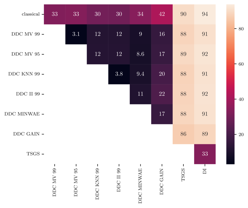
Figure 10: Relative spectral difference (in percentages) between estimated covariance matrices of the $11$ features of the R camera dataset.

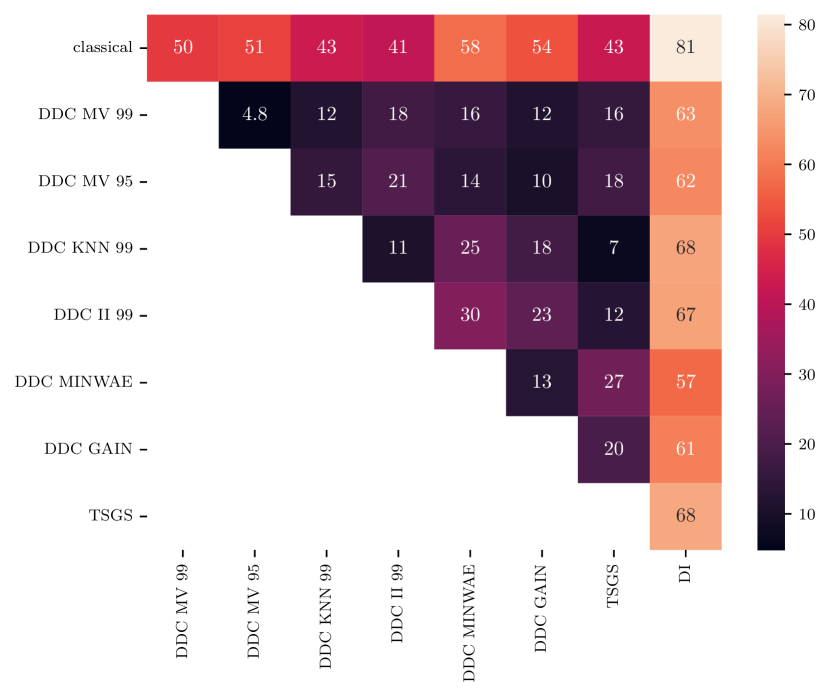
Figure 11: Relative spectral difference (in percentages) between estimated covariance matrices of the 30 features of sklearn’s Breast Cancer. DI disagrees with every other procedures, casting some doubt on the reliability of its estimate.

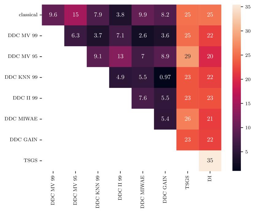
Figure 12: Relative spectral difference (in percentages) between estimated covariance matrices of the 11 features of the Woolridge Barium dataset.

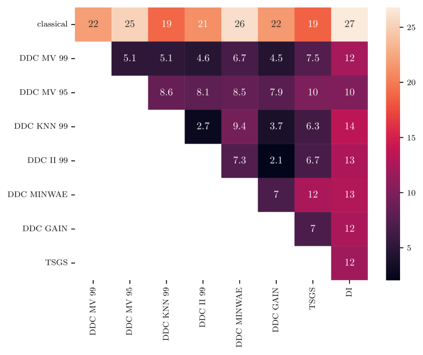
Figure 13: Relative spectral difference (in percentages) between estimated covariance matrices of the 13 features of sklearn’s Wine dataset.

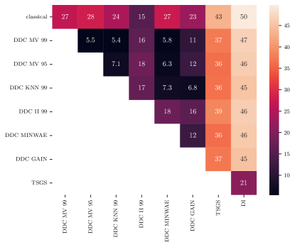
Figure 14: Relative spectral difference (in percentages) between estimated covariance matrices of the 13 features of Woolridge’s INTDEF dataset.

References

- [1] Pedro Abdalla and Nikita Zhivotovskiy. Covariance Estimation: Optimal Dimension-free Guarantees for Adversarial Corruption and Heavy Tails, July 2023.
- [2] Claudio Agostinelli, Andy Leung, Victor J. Yohai, and Ruben H. Zamar. Robust estimation of multivariate location and scatter in the presence of cellwise and casewise contamination, June 2014.
- [3] Fatemah Alqallaf, Stefan Van Aelst, Victor J. Yohai, and Ruben H. Zamar. Propagation of outliers in multivariate data. The Annals of Statistics, 37(1):311–331, February 2009.
- [4] Florentina Bunea and Luo Xiao. On the sample covariance matrix estimator of reduced effective rank population matrices, with applications to fPCA. Bernoulli, 21(2), May 2015.
- [5] Mengjie Chen, Chao Gao, and Zhao Ren. Robust Covariance and Scatter Matrix Estimation under Huber’s Contamination Model. arXiv:1506.00691 [math, stat], June 2017.
- [6] Mike Danilov, Victor Yohai, and Ruben Zamar. Robust Estimation of Multivariate Location and Scatter in the Presence of Missing Data. JASA. Journal of the American Statistical Association, 107, September 2012.
- [7] A. P. Dempster, N. M. Laird, and D. B. Rubin. Maximum Likelihood from Incomplete Data via the EM Algorithm. Journal of the Royal Statistical Society. Series B (Methodological), 39(1):1–38, 1977.
- [8] Sheela Devadas, Peter J Haine, and Keaton Stubis. The Schur-Horn Theorem. 2015.
- [9] Weinan Dong, Daniel Yee Tak Fong, Jin-sun Yoon, Eric Yuk Fai Wan, Laura Elizabeth Bedford, Eric Ho Man Tang, and Cindy Lo Kuen Lam. Generative adversarial networks for imputing missing data for big data clinical research. BMC Medical Research Methodology, 21(1):78, April 2021.
- [10] Alessio Farcomeni. Robust Constrained Clustering in Presence of Entry-Wise Outliers. Technometrics, 56, February 2014.
- [11] Peter J. Huber. Robust Estimation of a Location Parameter. The Annals of Mathematical Statistics, 35(1):73–101, 1964.
- [12] Peter J. Huber and Elvezio M. Ronchetti. Robust Statistics, 2nd Edition | Wiley. Wiley Series in Probability and Statistics. John Wiley and Sons, Inc., 2009.
- [13] Mia Hubert, Michiel Debruyne, and Peter J. Rousseeuw. Minimum Covariance Determinant and Extensions. WIREs Computational Statistics, 10(3), May 2018.
- [14] Mortaza Jamshidian and Peter M. Bentler. ML Estimation of Mean and Covariance Structures with Missing Data Using Complete Data Routines. Journal of Educational and Behavioral Statistics, 24(1):21–41, 1999.
- [15] Daniel Jarrett, Bogdan Cebere, Tennison Liu, Alicia Curth, and Mihaela van der Schaar. Hyperimpute: Generalized iterative imputation with automatic model selection. 2022.
- [16] Charles R. Johnson. Matrix theory and applications (charles r. johnson, ed.). Proceedings of symposia in applied mathematics, 40, 1989.
- [17] Julie Josse, Nicolas Prost, Erwan Scornet, and Gaël Varoquaux. On the consistency of supervised learning with missing values. arXiv:1902.06931 [cs, math, stat], July 2020.
- [18] Yegor Klochkov and Nikita Zhivotovskiy. Uniform Hanson-Wright type concentration inequalities for unbounded entries via the entropy method, August 2019.
- [19] Vladimir Koltchinskii and Karim Lounici. Asymptotics and concentration bounds for bilinear forms of spectral projectors of sample covariance. Annales de l’Institut Henri Poincaré, Probabilités et Statistiques, 52(4):1976 – 2013, 2016.
- [20] Vladimir Koltchinskii and Karim Lounici. Concentration inequalities and moment bounds for sample covariance operators. Bernoulli, 23(1):110–133, February 2017.
- [21] Vladimir Koltchinskii and Karim Lounici. New asymptotic results in principal component analysis. Sankhya A, 79(2):254–297, Aug 2017.
- [22] Vladimir Koltchinskii and Karim Lounici. Normal approximation and concentration of spectral projectors of sample covariance. The Annals of Statistics, 45(1):121 – 157, 2017.
- [23] Vladimir Koltchinskii, Karim Lounici, and Alexander B. Tsybakov. Estimation of Low-Rank Covariance Function, April 2015.
- [24] Andy Leung, Hongyang Zhang, and Ruben H. Zamar. Robust regression estimation and inference in the presence of cellwise and casewise contamination. Computational Statistics & Data Analysis, 99:1–11, July 2016.
- [25] Roderick Little and Donald Rubin. Statistical Analysis with Missing Data, Second Edition. Wiley Series in Probability and Mathematical Statistics. Probability and Mathematical Statistics. Wiley edition, 2002.
- [26] Karim Lounici. High-dimensional covariance matrix estimation with missing observations. Bernoulli, 20(3):1029–1058, August 2014.
- [27] Chao Ma, Sebastian Tschiatschek, José Miguel Hernández-Lobato, Richard Turner, and Cheng Zhang. VAEM: A Deep Generative Model for Heterogeneous Mixed Type Data, June 2020.
- [28] Pierre-Alexandre Mattei and Jes Frellsen. MIWAE: Deep Generative Modelling and Imputation of Incomplete Data Sets. In Kamalika Chaudhuri and Ruslan Salakhutdinov, editors, Proceedings of the 36th International Conference on Machine Learning, ICML 2019, 9-15 June 2019, Long Beach, California, USA, volume 97 of Proceedings of Machine Learning Research, pages 4413–4423. PMLR, 2019.
- [29] Alain Pajor. Metric Entropy of the Grassmann Manifold. Complex Geometry Analysis, 34:181–188, 1998.
- [30] F. Pedregosa, G. Varoquaux, A. Gramfort, V. Michel, B. Thirion, O. Grisel, M. Blondel, P. Prettenhofer, R. Weiss, V. Dubourg, J. Vanderplas, A. Passos, D. Cournapeau, M. Brucher, M. Perrot, and E. Duchesnay. Scikit-learn: Machine learning in Python. Journal of Machine Learning Research, 12:2825–2830, 2011.
- [31] Nikita Puchkin, Fedor Noskov, and Vladimir Spokoiny. Sharper dimension-free bounds on the Frobenius distance between sample covariance and its expectation, August 2023.
- [32] Jakob Raymaekers and Peter J. Rousseeuw. Handling cellwise outliers by sparse regression and robust covariance. arXiv:1912.12446 [stat], December 2020.
- [33] Jakob Raymaekers and Peter J. Rousseeuw. Fast robust correlation for high-dimensional data. Technometrics, 63(2):184–198, April 2021.
- [34] Peter J. Rousseeuw and Wannes Van den Bossche. Detecting deviating data cells. Technometrics, 60(2):135–145, April 2018.
- [35] Donald B. Rubin. Inference and Missing Data. Biometrika, 63(3):581–592, 1976.
- [36] Eckhard Schlemm. The kearns–saul inequality for bernoulli and poisson-binomial distributions. Journal of theoretical probability, 29:48–62, 2016.
- [37] R. C. Thompson. Principal submatrices of normal and Hermitian matrices. Illinois Journal of Mathematics, 10(2):296–308, June 1966.
- [38] Joel A. Tropp. An introduction to matrix concentration inequalities. Foundations and Trends® in Machine Learning, 8(1-2):1–230, 2015.
- [39] Olga Troyanskaya, Michael Cantor, Gavin Sherlock, Pat Brown, Trevor Hastie, Robert Tibshirani, David Botstein, and Russ B. Altman. Missing value estimation methods for DNA microarrays. Bioinformatics, 17(6):520–525, June 2001.
- [40] Alexandre B. Tsybakov. Nonparametric estimators. In Alexandre B. Tsybakov, editor, Introduction to Nonparametric Estimation, Springer Series in Statistics, pages 1–76. Springer, New York, NY, 2009.
- [41] John W. Tukey. The Ninther, a Technique for Low-Effort Robust (Resistant) Location in Large Samples. In H. A. David, editor, Contributions to Survey Sampling and Applied Statistics, pages 251–257. Academic Press, January 1978.
- [42] Stef van Buuren and Karin Groothuis-Oudshoorn. Mice: Multivariate Imputation by Chained Equations in R. Journal of Statistical Software, 45:1–67, December 2011.
- [43] Roman Vershynin. Introduction to the non-asymptotic analysis of random matrices, November 2011.
- [44] Roman Vershynin. High-Dimensional Probability: An Introduction with Applications in Data Science. Cambridge Series in Statistical and Probabilistic Mathematics. Cambridge University Press, Cambridge, 2018.
- [45] Vincent Q. Vu and Jing Lei. Minimax sparse principal subspace estimation in high dimensions. The Annals of Statistics, 41(6):2905–2947, December 2013.
- [46] Jeffrey M. Wooldridge. Introductory econometrics : a modern approach / Jeffrey M. Wooldridge,… Cengage learning, 2016.
- [47] Jinsung Yoon, James Jordon, and Mihaela van der Schaar. GAIN: Missing Data Imputation using Generative Adversarial Nets, June 2018.
- [48] Shuhan Zheng and Nontawat Charoenphakdee. Diffusion models for missing value imputation in tabular data, March 2023.