Emergence of ultradiscrete states due to phase lock
caused by saddle-node bifurcation in discrete limit cycles

Yoshihiro Yamazaki^1∗) and Shousuke Ohmori^2,3

¹Department of Physics, Waseda University, Shinjuku, Tokyo 169-8555, Japan
²National Institute of Technology, Gunma College, Maebashi-shi, Gunma 371-8530, Japan
³Waseda Research Institute for Science and Engineering, Waseda UniversityShinjuku, Tokyo 169-8555, Japan

*corresponding author : yoshy@waseda.jp
  

Abstract
Dynamical properties of limit cycles in a tropically discretized negative feedback model are numerically investigated. This model has a controlling parameter $\tau$, which corresponds to time interval for the time evolution of phase in the limit cycles. By considering $\tau$ as a bifurcation parameter, we find that ultradiscrete state emerges due to phase lock caused by saddle-node bifurcation. Furthermore, focusing on limit cycles for the max-plus negative feedback model, it is found that the unstable limit cycle in the max-plus model corresponds to the unstable fixed points emerging by the saddle-node bifurcation in the tropically discretized model.

Introduction: Limit cycles can be encountered in various systems as one of fundamental nonlinear phenomena[1], and various models have been proposed to reproduce limit cycles such as predator-prey model in ecological systems, negative feedback model and Fitzhugh-Nagumo model in biological systems, Sel’kov model in biochemical reactions, van der Pol equation in electric circuits. These models are mainly expressed in terms of continuous differential or discrete difference equations according to the time evolution of respective real phenomena. Furthermore, there also have been studies to derive max-plus equations for the above models by appropriate discretization and ultradiscretization, so that derived max-plus equations can be interpreted as cellular automata [2, 3, 4, 5, 6, 7, 8, 9]. The interesting point here is that derived max-plus equations can also possess similar limit cycle solutions to the continuous or discretized equations. Thus, it is important to clarify how the limit cycle structures are caused and are retained and how the limit cycles are ultradiscretized in discretized and max-plus systems.

As an appropriate discretization, tropical discretization is typically adopted. Here we briefly introduce the tropical discretization[10], which is a discretizing procedure converting a continuous differential equation into a discrete difference equation with only positive variables. Now we focus on a two-variable dynamical system having limit cycle solutions, and the following type of equations is treated for positive values of $x$ and $y$,

$$\frac{dx}{dt}=f_{1}(x,y)-g_{1}(x,y),\;\;\;\;\;\frac{dy}{dt}=f_{2}(x,y)-g_{2}(x,y),$$ (1)

where $f_{j}$ and $g_{j}$ are positive functions ($j=1,2$). The tropical discretization of eq. (1) is given as

$$x_{n+1}=x_{n}\frac{x_{n}+\tau f_{1}(x_{n},y_{n})}{x_{n}+\tau g_{1}(x_{n},y_{n})},\;\;\;\;\;y_{n+1}=y_{n}\frac{y_{n}+\tau f_{2}(x_{n},y_{n})}{y_{n}+\tau g_{2}(x_{n},y_{n})},$$ (2)

where $x_{n}=x(n\tau)$, $y_{n}=y(n\tau)$, and $\tau(>0)$ and $n$ show the discretized time interval and the number of iteration steps, respectively. Note that eq. (1) can be reproduced from eq. (2) by taking $\tau\rightarrow 0$.

For application of the tropical discretization to dynamical systems with limit cycle solutions, Carstea et al. treated the three dimensional model for a reaction of an organism to pathogen invasion and inflammatory response[11]. (They called it PRE model. P, R, and E stand for the initial letters of pathogens, responders, and effectors, respectively.) They reported that PRE model possesses limit cycle solutions and that the ultradiscrete max-plus equations obtained from the PRE model also have limit cycle solutions. Based on this study, Willox et al. further investigated dynamical properties of the limit cycles by the ultradiscretized PRE model[2]. They also investigated a two dimensional predator-prey model as a more simplified one by adopting Fourier spectrum analysis. They suggested that ultradiscrete limit cycles correspond to a limit case of the tropically discretized ones.

Gibo and Ito studied a negative feedback model[3]. For the continuous negative feedback model, it has been confirmed that there is no limit cycle solution[12]. However they showed that the tropically discretized negative feedback model exhibits Neimark-Sacker bifurcation and has limit cycle solutions[3]. They pointed out that in some biological systems, the discrete model with limit cycles is better suited to real phenomena. Furthermore, they derived the max-plus negative feedback model and numerically showed the existence of the attractive ultradiscre limit cycle, which consists of four states. Based on the study of Gibo and Ito, we further investigated the dynamical properties of these negative feedback models[8] and showed emergence of the ultradiscre limit cycle for large $\tau$. And by using the Poincaré map method, we found that the max-plus model has the two limit cycles, stable (attractive) and unstable (repulsive).

We have also investigated dynamical properties of limit cycles obtained from Sel’kov model [13, 5, 6, 7]. We confirmed that ultradiscrete states emerge for large $\tau$ in the tropically discretized Sel’kov model. Also we found that there exist not only a stable limit cycle but also an unstable one in the max-plus equations obtained via ultradiscretization in the limit of $\tau\to\infty$. These properties are essentially the same as those of the negative feedback models shown above.

In view of these previous studies, it is important to advance analysis for the dynamical properties of the limit cycles in these discrete models. Actually, the previous analyses seem to be insufficient especially for understanding emergence of ultradiscrete states in tropically discretized systems. And relationship between limit cycle states obtained from tropically discretized and max-plus models is not clear. Furthermore, there is no explanation for existence of the unstable limit cycle solutions in the max-plus models. In this letter, focusing on limit cycle solutions of the tropically discretized negative feedback model, we show one scenario of how ultradiscretized states emerge in the limit cycles with $\tau$ as a bifurcation parameter from the viewpoint of bifurcation phenomena. And we discuss the correspondence with the limit cycles obtained from the max-plus negative feedback model.

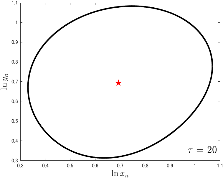
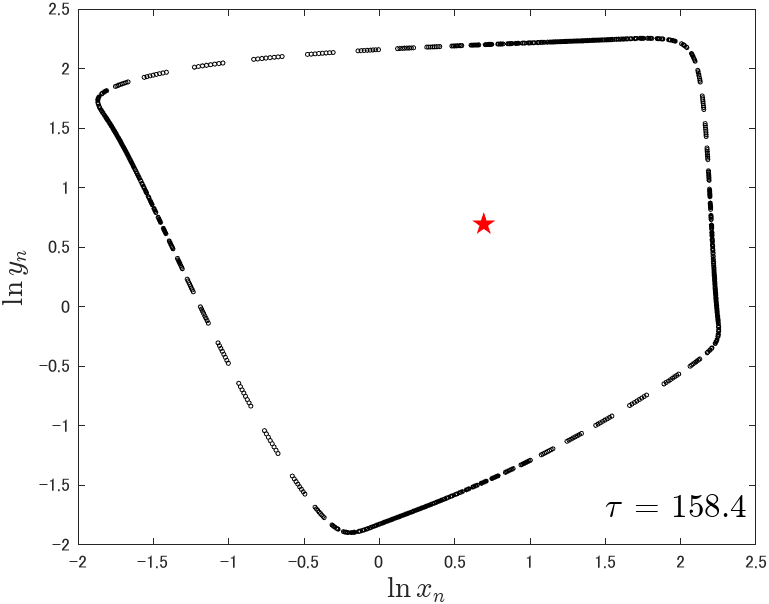
(a)                                                          (b)

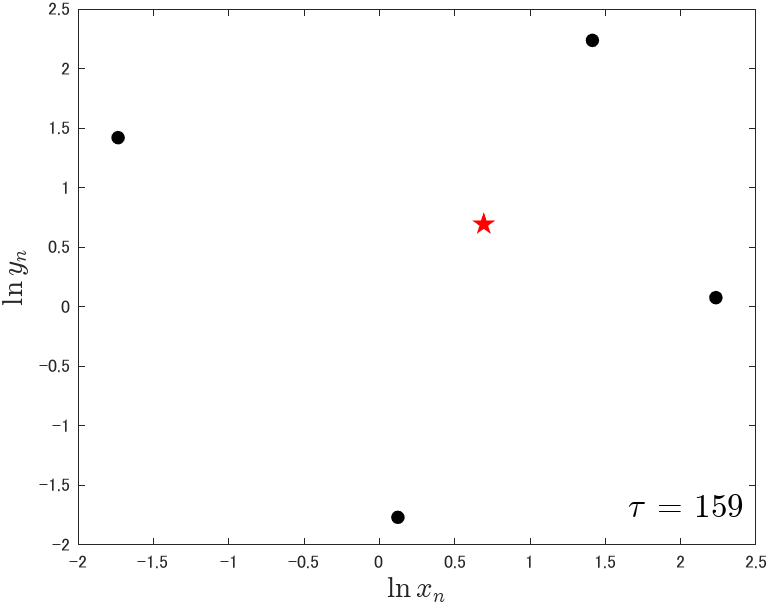
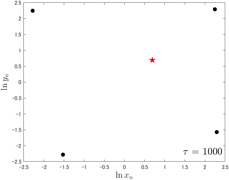
(c)                                                          (d)

Figure 1: The limit cycles obtained from eq.(3) with $b=10$ and $m=2$. The values of $\tau$ are (a) 20, (b) 158.4, (c) 159, and (d) 1000. In (c) and (d), the limit cycles consist of the four states, which are depicted by the black filled cirlces. These are plotted with log-log scales. The red star in each figure shows the fixed point $(\bar{x},\bar{y})=(2,2)$.

Modelling and numerical results: Let us start with introducing the tropically discretized negative feedback model for $(x_{n},y_{n})$[3, 8]:

$$x_{n+1}=\frac{x_{n}+\tau y_{n}}{1+\tau}\equiv\eta_{\tau}(x_{n},y_{n}),\;\;\;\;y_{n+1}=\frac{y_{n}+\frac{\tau}{1+x_{n}^{m}}}{1+\frac{\tau}{b}}\equiv\xi_{\tau}(x_{n},y_{n}),$$ (3)

where $b$ and $m$ are positive parameters. We set $m=2$ and $b=10$ hereafter for numerical calculation, which was done by using Mathematica and MATLAB. Note that the original continuous equations for eq.(3), $dx/dt=y-x$ and $dy/dt=1/(1+x^{m})-y/b$, possess the unique stable fixed point and there is no limit cycle solution[12]. On the other hand, following the previous results in refs.[3, 8, 14], eq.(3) exhibits Neimark-Sacker bifurcation at $\tau=\tau_{0}=\frac{b(b+1)}{(m-1)b-m\bar{x}}=\frac{55}{3}$, and has a limit cycle solution for $\tau>\tau_{0}$ even in the limit of $\tau\to+\infty$. Figure 1 shows examples of the limit cycles with four different values of $\tau$. It is found that as $\tau$ increases phase states in the limit cycles tend to be sparsely distributed and finally converge to the four states, which correspond to the ultradiscrete states. These results are consistent with our previous study[8].

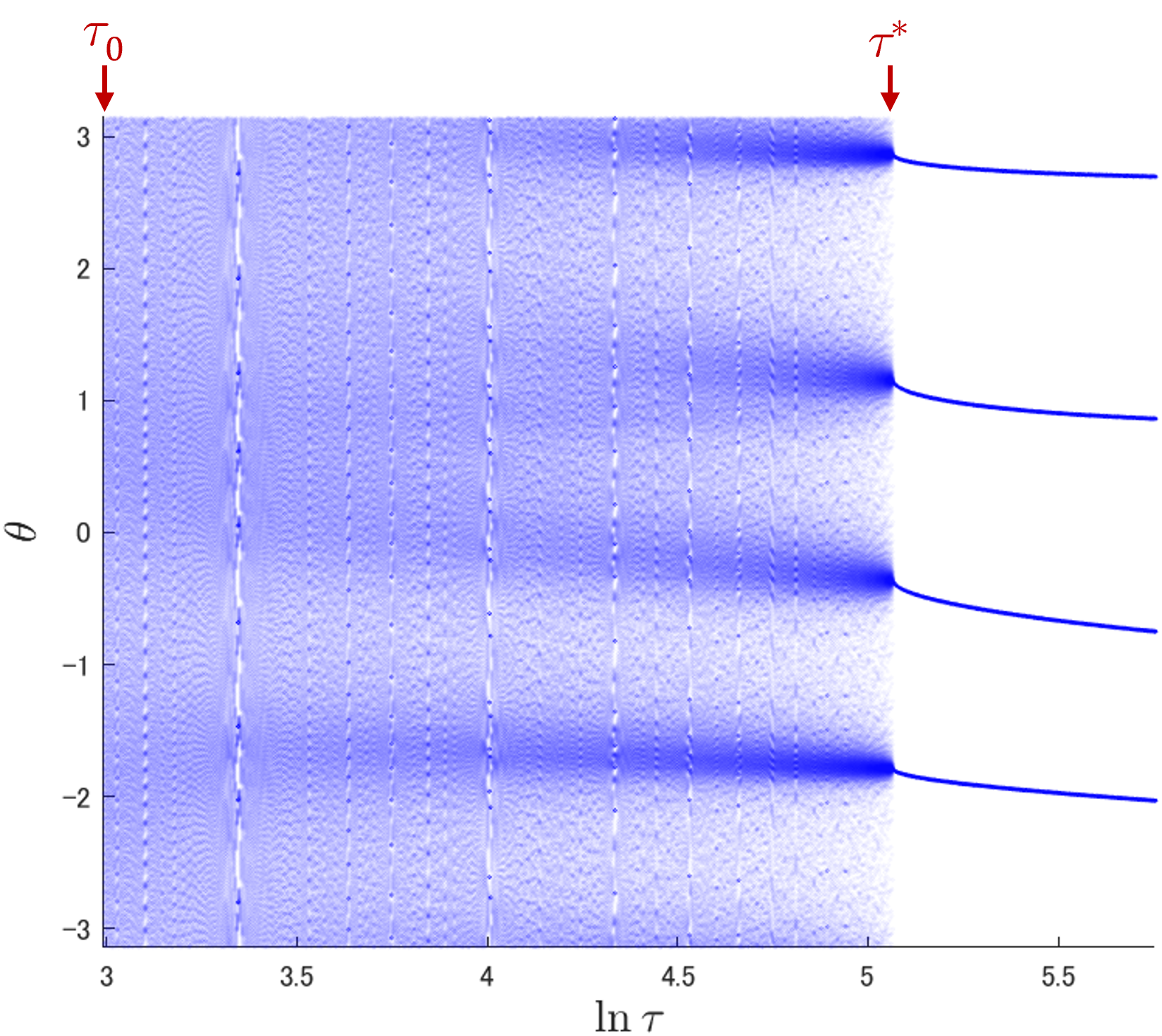
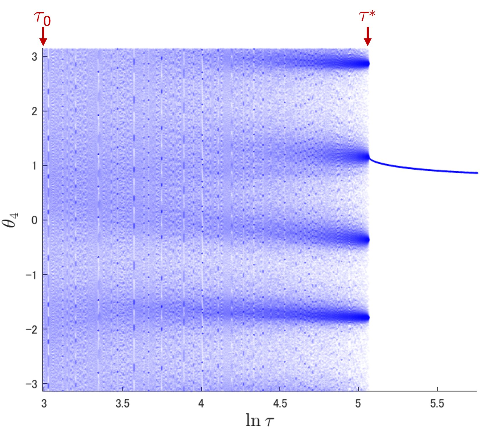
(a)                                                          (b)

Figure 2: (a) The scatter plot of the phase $\{\theta_{n}(\tau)\}$ in the limit cycles, where $m=2$ and $b=10$. $\theta_{n}(\tau)$ is defined as eq.(4). (b) The scatter plot of the phase $\{\theta_{4n}(\tau)\}$. In both figures, 500 points are plotted at each value of $\tau$.

For the state $(x_{n},y_{n})$ in the limit cycle, we define the phase $\theta_{n}(\tau)$ as

$$\theta_{n}(\tau)=\arctan\displaystyle\frac{\ln y_{n}-\ln\bar{y}}{\ln x_{n}-\ln\bar{x}},$$ (4)

which takes a value in the range of $[-\pi,+\pi]$. Figure 2(a) shows the scatter plot of $\{\theta_{n}(\tau)\}$ in the limit cycles as a function of $\tau$. It is clearly found that distribution of $\{\theta_{n}(\tau)\}$ drastically changes at a certain value of $\tau$, denoted by $\tau^{\ast}$ in Fig. 2. Note that Fig. 2(a) can be considered as a bifurcation diagram of $\{\theta_{n}(\tau)\}$ for eq.(3), and the change at $\tau=\tau^{\ast}$ suggests transition between discrete and ultradiscrete limit cycles. Since the ultradiscrete limit cycle consists of four states, we focus on the phase state distribution of every four steps, $\{\theta_{4n}\}(n=1,2,3,\cdots)$ as shown in Fig.2(b). $\{\theta_{4n}\}$ is obtained from 4-th iterates of $\eta_{\tau}$ and $\xi_{\tau}$, denoted by $\eta^{4}_{\tau}$ and $\xi^{4}_{\tau}$. In Fig. 2(b), the value of $\{\theta_{4n}\}$ for $\tau>\tau^{\ast}$ corresponds to one of the stable fixed points for

$$x_{4(n+1)}=\eta^{4}_{\tau}(x_{4n},y_{4n}),\;\;\;\;y_{4(n+1)}=\xi^{4}_{\tau}(x_{4n},y_{4n}).$$ (5)

Actually except for $(\bar{x},\bar{y})$, we find eight fixed points $(\bar{x}_{4},\bar{y}_{4})$, which are obtained from $\bar{x}_{4}=\eta^{4}_{\tau}(\bar{x}_{4},\bar{y}_{4})$ and $\bar{y}_{4}=\xi^{4}_{\tau}(\bar{x}_{4},\bar{y}_{4})$ when $\tau>\tau^{\ast}$, whereas there is no fixed point for $\tau<\tau^{\ast}$. The value of $\tau^{\ast}$ was numerically estimated as $\tau^{\ast}\approx 158.7137871989345$ from the change in the number of the fixed points. Furthermore, it is found that four of the eight fixed points coincide with the four lines shown in Fig.2(a) for $\tau>\tau^{\ast}$. Now we denote these four points as $\{\bar{\theta}_{4}^{\rm{(s)}}(\tau)\}$, and the rest four are denoted as $\{\bar{\theta}_{4}^{\rm{(u)}}(\tau)\}$, which are identified later. Figure 3 shows the fixed points $\{\bar{\theta}_{4}^{\rm{(s)}}\}$ (blue filled circles) and $\{\bar{\theta}_{4}^{\rm{(u)}}\}$ (red open circles) as a function of $\tau$. It is found from this figure that each value in $\{\bar{\theta}_{4}^{\rm{(s)}}\}$ is paired with one value in $\{\bar{\theta}_{4}^{\rm{(u)}}\}$, and they coalesce and vanish at $\tau=\tau^{\ast}$.

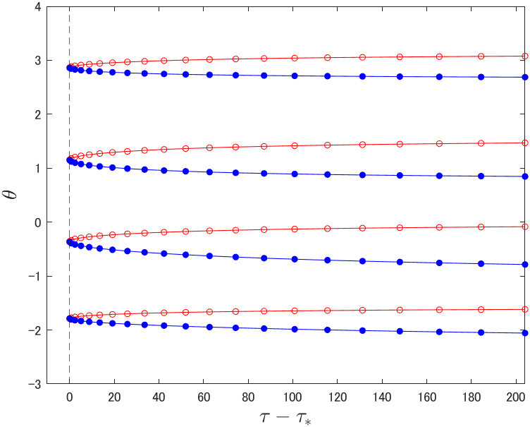
Figure 3: Phase description of the eight fixed points $\{\bar{\theta}_{4}^{\rm{(s)}}\}$ (blue filled circles) and $\{\bar{\theta}_{4}^{\rm{(u)}}\}$ (red open circles) as a function of $\tau(>\tau^{\ast})$.

Next we focus on the eigenvalues of Jacobi matrix for the eight values of $(\bar{x}_{4},\bar{y}_{4})$ when $\tau>\tau^{\ast}$. It is confirmed that the eigenvalues of each fixed point in $\{\bar{\theta}_{4}^{\rm{(s)}}\}$ are the same, and the same is also true for $\{\bar{\theta}_{4}^{\rm{(u)}}\}$. Figure 4(a) shows the maximum eigenvalues $\lambda_{4}^{\rm{(s)}}$ for $\{\bar{\theta}_{4}^{\rm{(s)}}\}$ and $\lambda_{4}^{\rm{(u)}}$ for $\{\bar{\theta}_{4}^{\rm{(u)}}\}$ as a function of $\tau$. Red asterisks and blue circles correspond to $\lambda_{4}^{\rm{(u)}}$ and $\lambda_{4}^{\rm{(s)}}$, respectively. It is found that $\{\bar{\theta}_{4}^{\rm{(s)}}\}$ are stable and $\{\bar{\theta}_{4}^{\rm{(u)}}\}$ are unstable since $\lambda_{4}^{\rm{(s)}}<1$ and $\lambda_{4}^{\rm{(u)}}>1$ for all $\tau>\tau^{\ast}$. Furthremore it is found that $\lambda_{4}^{\rm{(s)}}$ and $\lambda_{4}^{\rm{(u)}}$ tend to become 1 as $\tau$ goes to $\tau^{\ast}+0$. Therefore, saddle-node bifurcation occurs at $\tau=\tau^{\ast}$. Note that as an asymptotic property for $\tau$ dependence of $\lambda_{4}^{\rm{(s)}}$ and $\lambda_{4}^{\rm{(u)}}$, the following scaling relations are confimed as shown in Fig. 4(b): $|\lambda_{4}^{\rm{(s)}}-1|,|\lambda_{4}^{\rm{(u)}}-1|\sim(\tau-\tau^{\ast})^{0.5}$. From this bifurcation analysis, it is concluded that the ultradiscrete states in the limit cycle of the tropically discretized negative feedback model emerge due to phase lock by saddle-node bifurcation at $\tau=\tau^{\ast}$.

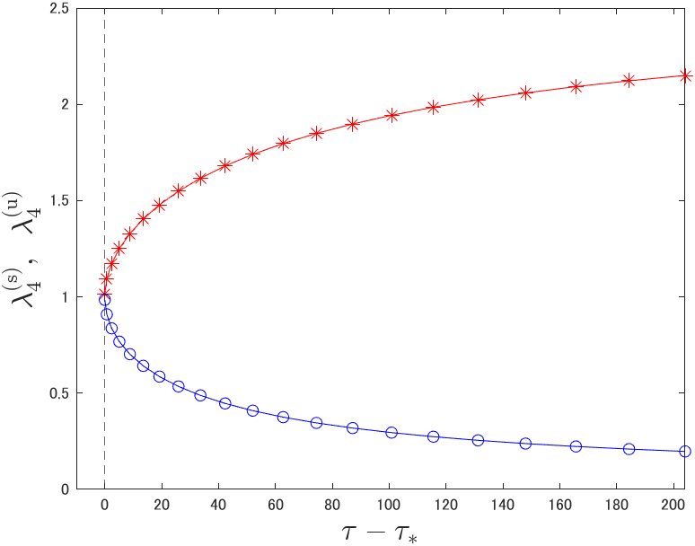
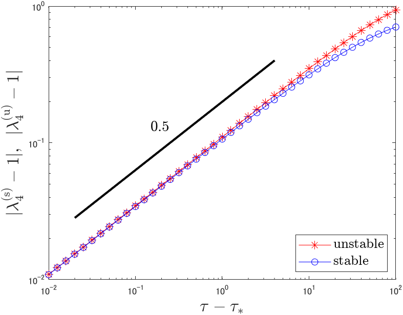
(a)                                                          (b)

Figure 4: (a) The maximum eigenvalues $\lambda_{4}^{\rm{(s)}}$ for $\{\bar{\theta}_{4}^{\rm{(s)}}\}$ and $\lambda_{4}^{\rm{(u)}}$ for $\{\bar{\theta}_{4}^{\rm{(u)}}\}$ as a function of $\tau(>\tau^{\ast})$. (b) The log-log plot of (a). The thick black line segment shows the guide line, whose slope is 0.5.

Discussion: (i) First we comment on an additional meaning of the tropical discretization. One of the equations in eq.(2) can be rewritten as

$$x_{n+1}=r_{n}(\tau)x_{n},\;\;\;\;r_{n}(\tau)\equiv\frac{1+\tau\frac{f_{1}(x_{n},y_{n})}{x_{n}}}{1+\tau\frac{g_{1}(x_{n},y_{n})}{x_{n}}}.$$ (6)

This equation for $x_{n}$ can be interpreted as a multiplicative time evolution from $x_{n}$ to $x_{n+1}$, where $r_{n}$ is the change ratio. $f_{1}$ and $g_{1}$ in $r_{n}$ are considered as magnification and reduction factors, respectively. $\tau$ can be treated as a coefficient controlling the degree of magnification and reduction. Therefore, the tropical discretization seems to be suitable for discrete modeling of multiplicative processes, which is in contrast to an additive discretization such as Euler difference method.

(ii) When $\tau<\tau^{\ast}$ in eq.(3), we found that $\theta_{4n}$ exhibits phase drift and bottleneck motion as shown in Fig.5(a)-(e). Especially as $\tau$ approaches $\tau^{\ast}-0$, time to pass through the bottlenecks, which is defined as $T_{\rm{b.n.}}$ in Fig.5(d), becomes longer. In fact as shown in Fig.5(f), $T_{\rm{b.n.}}$ is subject to the scaling relation: $T_{\rm{b.n.}}\sim(\tau^{\ast}-\tau)^{-0.5}$. Note that this scaling relation is well-known as the standard property in the vicinity of saddle-node bifurcation point[1]. Therefore, this slowing down in phase drift motion for $\tau\lesssim\tau^{\ast}$ also supports occurrence of saddle-node bifurcation at $\tau=\tau^{\ast}$.

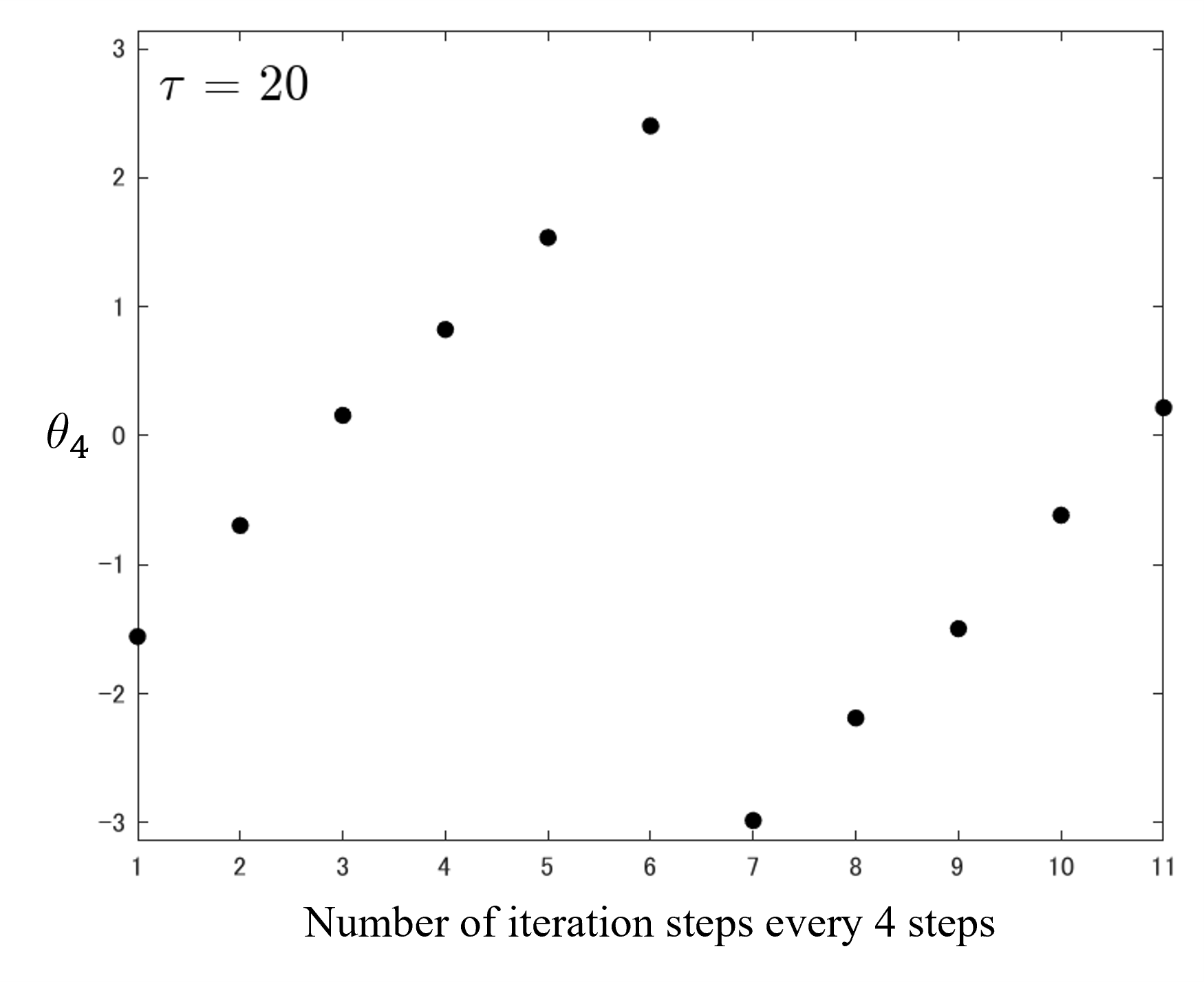
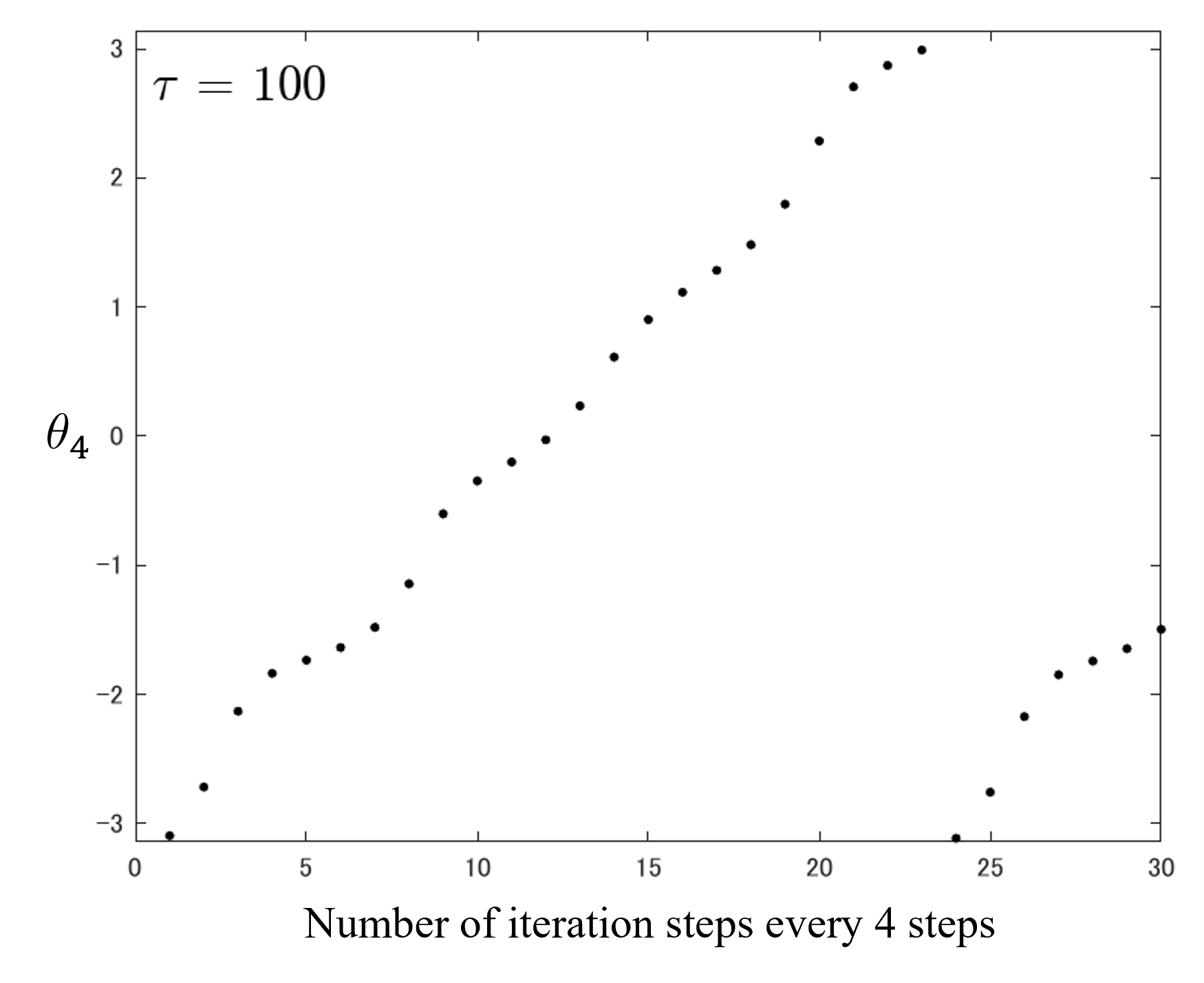
(a)                                                          (b)

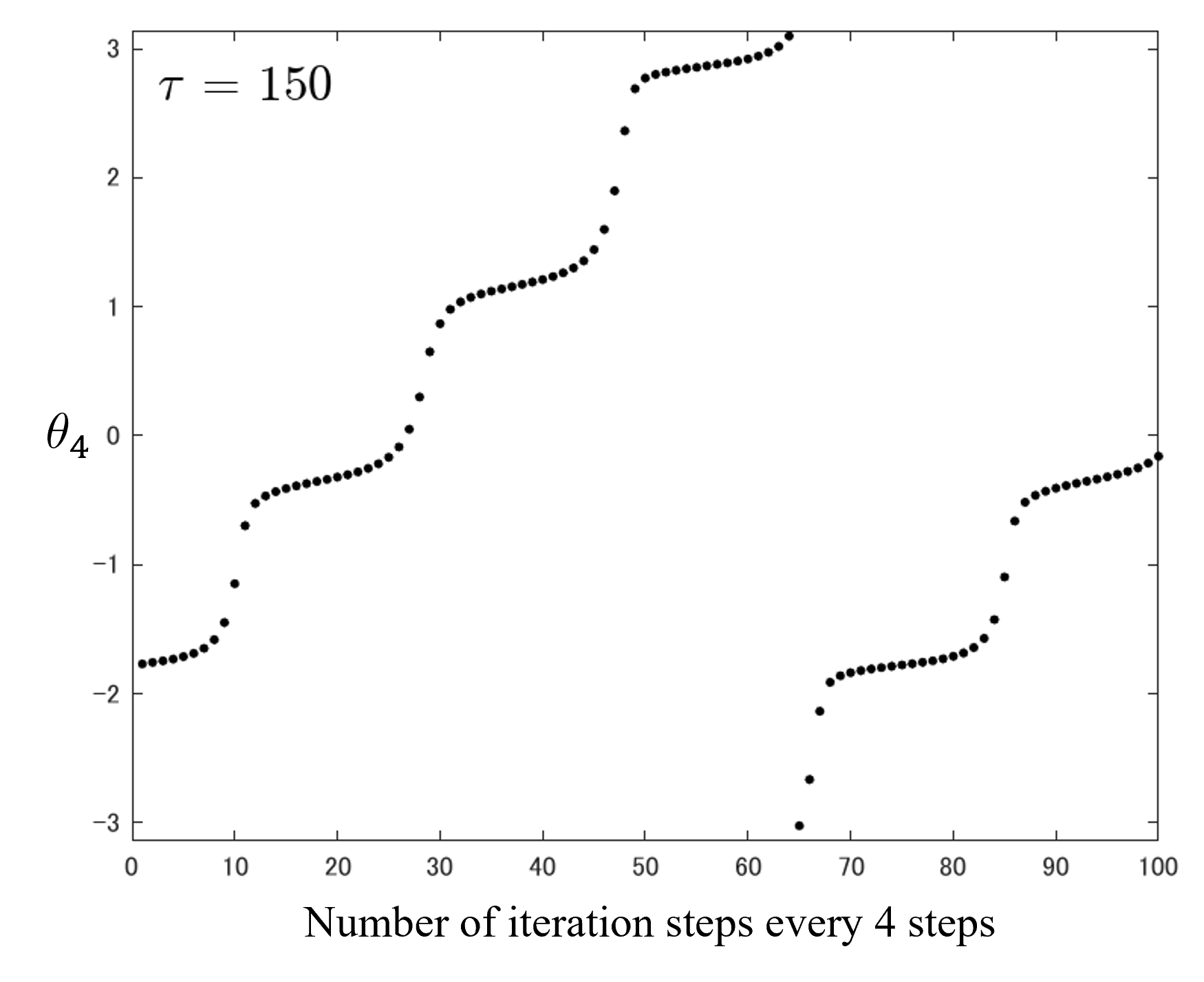
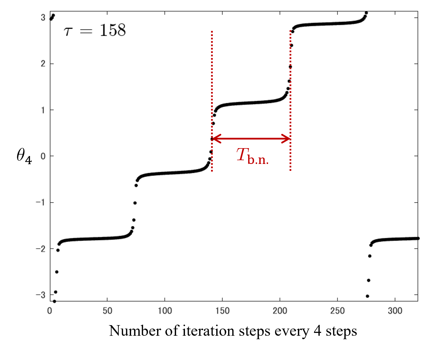
(c)                                                          (d)

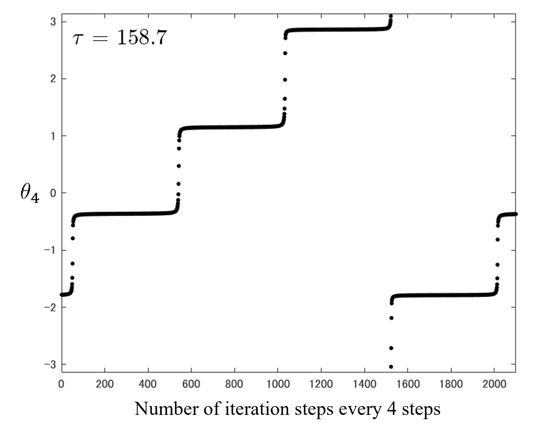
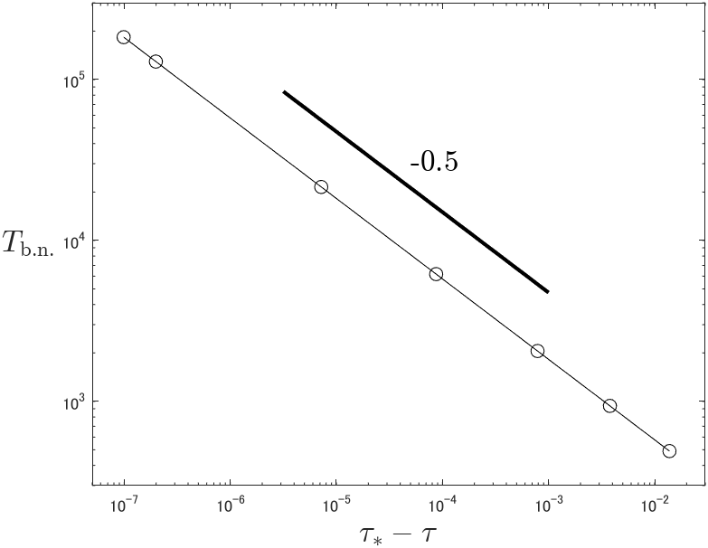
(e)                                                          (f)

Figure 5: (a)-(e) Time evolutions of $\theta_{4n}$ with five different values of $\tau$, where $b=10$ and $m=2$. (f) Scaling relation between $\tau^{\ast}-\tau$ and $T_{\rm{b.n.}}$, which is defined as shown in (d).

(iii) The present results and conlusion are obtained from analysis of a specific model, the negative feedback model. Similar tendency has been suggested for the Sel’kov model as well[5, 6, 7]. Then the generality of this conclusion is expected, although further investigation is needed. The introduction of phase in the analysis of limit cycles has long been a basic and usual method in nonlinear dynamics[15]. The present study shows that the analysis on the basis of phase is also effective in the context of ultradiscretization, and it is interesting and important to review the study of Willox et al. [2] from the viewpoint of phase dynamics.

(iv) Here we discuss relationship between limit cycle solutions obtained from eq.(3) and those obtained from the max-plus equations, which are derived from eq.(3). Here in order to derive the max-plus equations from the discretized equations, we adopt the following replacement:

$$\displaystyle\log(e^{A_{1}}+e^{A_{2}})\to\max(A_{1},A_{2}),$$ (7)

where $A_{1}$ and $A_{2}$ are positive variables. It is noted that eq.(7) brings about piecewise linearization for the left hand side of eq.(7), and is mathematically formulated as the limit identity by introducing an additional scaling parameter[16]. Introducing new variables $X_{n}\equiv\ln x_{n}$, $Y_{n}\equiv\ln y_{n}$, $B\equiv\ln b$, and $T\equiv\ln\tau$ in eq.(3), and applying eq.(7), we obtain the following max-plus equations.

$$X_{n+1} =\max(X_{n},T+Y_{n})-\max(0,T),$$ (8)

$$Y_{n+1} =\max(Y_{n},T-\max(0,mX_{n}))-\max(0,T-B).$$

Performing numerical calculation of eq.(8), we confirmed that eq.(8) can possess cyclic solutions. Then we introduce phase $\Theta_{n}$, which is defined as

$$\Theta_{n}=\arctan\displaystyle\frac{Y_{n}-\ln\bar{y}}{X_{n}-\ln\bar{x}}.$$ (9)

The red lines in Fig. 6(a) show scatter plot of $\{\Theta_{n}\}$ as a function of $\tau$, where the result shown in Fig.2(a) is also superimposed on this figure. For $\tau<\tau^{\ast}$, the phases obtained from eq.(3) are broadly distributed and do not agree with the results obtained from eq.(8). However for $\tau>\tau^{\ast}$, both limit cycles consist of four states, and we can confirm a quantitative trend toward agreement in the phase values as $\tau$ increases. Actually, in Fig. 6(b), as $\tau$ increases, the states obtained by eq.(3) approach the states obtained from eq.(8). Note that for $B$ being finite, even when $\tau$ goes to infinity, the states by eq.(3) do not exactly match the states by eq.(8) quantitatively due to piecewise linearization by eq.(7). Nevertheless, even when $\tau>\tau^{\ast}$ and $B$ is finite, it is meaningful to express the states by the max-plus equations in order to construct corresponding cellular automata.

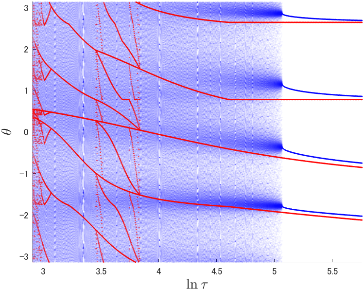
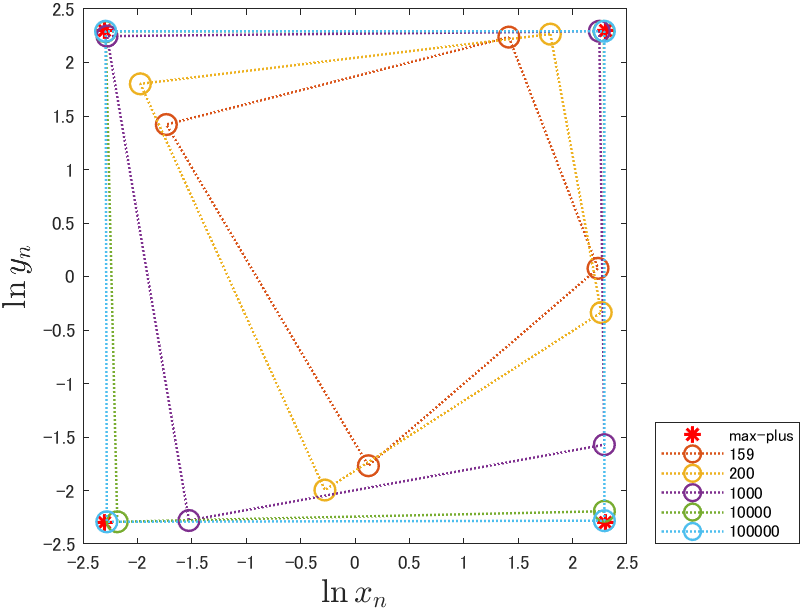
(a)                                                          (b)

Figure 6: (a) The red plots show $\{\Theta_{n}\}$ as a function of $\tau$ obtained from eq.(8), where $m=2$ and $B=\ln b=\ln 10$. For each $\tau$, 500 points are plotted. The superimposed blue scatterd plot is the same as Fig.2(a). (b) The open circles show limit cycle states with five different values of $\tau>\tau^{\ast}$. The asterisks show the limit cycle states obtained from eq.(8).

(v) Here we consider the limit case of $\tau\to\infty$ ($T\to\infty$). In this case, eq.(3) and eq.(8) can be rewritten as

$$x_{n+1}=y_{n}\equiv\eta_{\infty}(x_{n},y_{n}),\;\;\;\;y_{n+1}=\frac{b}{1+x_{n}^{m}}\equiv\xi_{\infty}(x_{n},y_{n}),$$ (10)

$$X_{n+1}=Y_{n},\;\;\;\;Y_{n+1}=B-\max(0,mX_{n}).$$ (11)

From our previous study[8], it has been confirmed that there exist the two limit cycle solutions in eq.(11), $\mathcal{C}$ and $\mathcal{C}_{s}$, which consist of the following four states, $\displaystyle\mathcal{C}$: $(\pm B,\pm B)$ and $\displaystyle\mathcal{C}_{s}$: $\displaystyle\left(\frac{B}{3},\pm B\right)$ and $\displaystyle\left(\pm B,\frac{B}{3}\right)$ for $m=2$. The important point is that $\mathcal{C}_{s}$ is the unstable repulsive limit cycle. Meanwhile, we focus on the fixed points for 4-th iterates of eq.(10), $(\bar{x}_{4\infty},\bar{y}_{4\infty})$, which are obtained from $\bar{x}_{4\infty}=\eta^{4}_{\infty}(\bar{x}_{4\infty},\bar{y}_{4\infty})$ and $\bar{y}_{4\infty}=\xi^{4}_{\infty}(\bar{x}_{4\infty},\bar{y}_{4\infty})$. We numerically obtained the eight fixed points, from which $(\ln\bar{x}_{4\infty},\ln\bar{y}_{4\infty})$ can be classified as $\mathcal{D}$: $(\pm\alpha,\pm\alpha)$ and $\mathcal{D}_{s}$: $(\beta,\pm\alpha)$ and $(\pm\alpha,\beta)$, where $\alpha$ and $\beta$ depend on the value of $B=\ln b$ as shown in Tbl.1. It is found from Tbl.1 that as $B$ increases, $\alpha$ and $\beta$ tend to $B$ and $B/3$, respectively. Therefore, it is suggested that $\mathcal{D}\to\mathcal{C}$ and $\mathcal{D}_{s}\to\mathcal{C}_{s}$ when $B\to\infty$ and $T\to\infty$; this is consistent with arguments based on ultradiscrete limit formula[16]. We can say that $\mathcal{C}_{s}$ is the inheritance of $\mathcal{D}_{s}$ and the remnant of unstable fixed points caused by saddle-node bifurcation. This result provides support for the fact that the dynamical structures of eq.(3) are retained even in the simple max-plus form of eq.(11).

Table 1: Comparison of $\alpha$ and $\beta$ obtained from numerical calculation of eq.(10) with the value of $B$. For $B-\alpha$ and $B/3-\beta$, only the orders are presented.

$b$	$B=\ln b$	$\alpha$	$\beta$	$B-\alpha$	$B/3-\beta$
$10^{1}$	2.3025$\cdots$	2.2924$\cdots$	0.6931$\cdots$	$10^{-2}$	$10^{-2}$
$10^{3}$	6.9077$\cdots$	6.9077$\cdots$	2.2992$\cdots$	$10^{-6}$	$10^{-3}$
$10^{5}$	11.5129$\cdots$	11.5129$\cdots$	3.8374$\cdots$	$10^{-10}$	$10^{-4}$
$10^{7}$	16.1180$\cdots$	16.1180$\cdots$	5.3726$\cdots$	$10^{-14}$	$10^{-6}$
$10^{9}$	20.7232$\cdots$	20.7232$\cdots$	6.9077$\cdots$	$10^{-18}$	$10^{-7}$

Summary and Conclusion: We have investigated dynamical properties of the limit cycles for the tropically discretized negative feedback model. Based on the bifurcation analysis with phase description, it is found that the limit cycle becomes ultradiscrete state with four states due to phase lock caused by saddle-node bifurcation at $\tau=\tau^{\ast}$, where $\tau$ behaves as the bifurcation parameter. We have discussed relationship between limit cycle states obtained from tropically discretized and the max-plus models, and it is also found that the unstable limit cycle $\mathcal{C}_{s}$ in the max-plus model corresponds to the unstable fixed points $\mathcal{D}_{s}$ appearing by the saddle-node bifurcation in the tropically discretized model.

Acknowledgement
The authors are grateful to Prof. M. Murata, Prof. K. Matsuya, Prof. D. Takahashi, Prof. R. Willox, Prof. T. Yamamoto, and Prof. Emeritus A. Kitada for useful comments and encouragements. This work was supported by JSPS KAKENHI Grant Numbers 22K13963 and 22K03442.

References

- [1] S. H. Strogatz, Nonlinear Dynamics and Chaos (Westview Press, U.S. 1994).
- [2] R. Willox, A. Ramani, J. Satsuma, and B. Grammaticos, Physica A 385 473 (2007).
- [3] S. Gibo and H. Ito, J. Theor. Biol., 378 89 (2015).
- [4] S. Ohmori and Y. Yamazaki, J. Phys. Soc. Jpn. 85 045001 (2016).
- [5] S. Ohmori and Y. Yamazaki, arXiv:2107.02435v1
- [6] Y. Yamazaki and S. Ohmori, J. Phys. Soc. Jpn. 90 103001 (2021).
- [7] S. Ohmori and Y. Yamazaki, JSIAM Letters 14, 127 (2022).
- [8] S. Ohmori and Y. Yamazaki, arXiv:2305.05908.
- [9] S. Isojima and S. Suzuki, Nonlinearity. 35 1468 (2022).
- [10] M. Murata, J. Differ. Equations Appl. 19 1008 (2013).
- [11] A. S. Carstea, A. Ramani, J. Satsuma, R. Willox, and B. Grammaticos, Physica A 364 276 (2006).
- [12] J. S. Griffith, J. Theor. Biol. 20, 202 (1968).
- [13] E. E. Sel′kov, Eur. J. Biochem. 4 79 (1968).
- [14] S. Ohmori and Y. Yamazaki, arXiv:2304.01573.
- [15] Y. Kuramoto, Chemical Oscillations, Waves, and Turbulence (Dover Publications, New York, 2003).
-
[16]
For deriving max-plus description,
it is common to apply the ultradiscrete limit formula
expressed in the following equation
instead of eq.(7) [17].
Here is the additional scaling parameter, and changing this value corresponds to controlling the scale of viewing the systems. And taking this value to infinity corresponds to the limit of zooming out, which brings about piecewise linearization. If we set , , , and in eq.(3), and applying the above ultradiscrete limit formula, we obtain the same max-plus equations as eq.(8). In the main text, it can be said that the case is considered. - [17] T. Tokihiro, Discrete Integrable Systems (edited by B. Grammaticos, T. Tamizhmani, and Y. Kosmann-Schwarzbach, Springer, Berlin, Heidelberg, 2004), pp. 383–424.