Neural Bee Colony Optimization: A Case Study in Public Transit Network Design
Abstract
In this work we explore the combination of metaheuristics and learned neural network solvers for combinatorial optimization. We do this in the context of the transit network design problem, a uniquely challenging combinatorial optimization problem with real-world importance. We train a neural network policy to perform single-shot planning of individual transit routes, and then incorporate it as one of several sub-heuristics in a modified Bee Colony Optimization (BCO) metaheuristic algorithm. Our experimental results demonstrate that this hybrid algorithm outperforms the learned policy alone by up to 20% and the original BCO algorithm by up to 53% on realistic problem instances. We perform a set of ablations to study the impact of each component of the modified algorithm.
1 Introduction
The design of urban transit networks is an important real-world problem, but is computationally very challenging. It has some similarities with other combinatorial optimization (CO) problems such as the Travelling Salesman problem (TSP) and Vehicle Routing Problem (VRP), but due to its many-to-many nature, combined with the fact that demand can be satisfied by transfers between transit lines, the problem is much more complex than those well-studied problems. The most successful approaches to the Transit Network Design Problem (NDP) to-date have been metaheuristic algorithms. Metaheuristics are high-level approximate strategies for problem-solving that are agnostic to the kind of problem. Many are inspired by natural phenomena, such as Simulated Annealing (SA), Genetic Algorithm (GA), and Bee Colony Optimization (BCO).
Metaheuristic algorithms have proven useful and remain the state-of-the-art in several very complex optimization problems (Ahmed et al., 2019). But little cross-over exists between the literature on this problem and that of machine learning with neural networks. In this work, we use a neural network system to learn low-level heuristics for the NDP, and use these learned heuristics in a metaheuristic algorithm. We show that this synthesis of a machine learning approach and meta-heuristic approach outperforms either of them alone.
We first develop a novel Graph Neural Network (GNN) policy model and train it in an Reinforcement Learning (RL) context to output transit networks that minimize an established cost function. We compare the performance of the trained GNN model to that of Nikolić and Teodorović (2013)’s BCO approach on a standard benchmark of NDP instances (Mumford, 2013a), characterizing them over a range of different cost functions. We then integrate this model into a metaheuristic algorithm called BCO, as one of the heuristics that the algorithm can employ as it performs a stochastic search of the solution space. We compare this approach to the GNN model and the unmodified BCO algorithm, and we find that on realistically-sized problem instances, the combination outperforms the GNN by up to 20% and BCO by up to 53%. Lastly, we perform several ablations to understand the importance of different components of the proposed system to its performance.
2 Related Work
2.1 Graph Networks and Reinforcement Learning for Optimization Problems
Graph Neural Networks (GNNs) are neural network models that are designed to operate on graph-structured data (Bruna et al., 2013; Kipf and Welling, 2016; Defferrard et al., 2016; Duvenaud et al., 2015). They were inspired by the success of convolutional neural nets on computer vision tasks and have been applied in many domains, including analyzing large web graphs (Ying et al., 2018), designing printed circuit boards (Mirhoseini et al., 2021), and predicting chemical properties of molecules (Duvenaud et al., 2015; Gilmer et al., 2017). An overview of GNNs is provided by Battaglia et al. (2018).
There has recently been growing interest in the application of machine learning techniques to solve CO problems such as the TSP and VRP (Bengio et al., 2021). As many such problems have natural interpretations as graphs, a popular approach has been to use GNNs to solve them. A prominent early example is the work of Vinyals et al. (2015), who propose Pointer Networks and train them via supervised learning to solve TSP instances.
In CO problems generally, it is difficult to find a globally optimal solution but easier to compute a scalar quality metric for any given solution. As noted by Bengio et al. (2021), this makes RL, in which a system learns to maximize a scalar reward, a natural fit. Recent work (Dai et al., 2017; Kool et al., 2019; Lu et al., 2019; Sykora et al., 2020) has used RL to train GNN models and have attained impressive performance on the TSP, the VRP, and related problems.
The solutions from some neural methods come close to the quality of those from specialized TSP algorithms such as Concorde (Applegate et al., 2001), while requiring much less run-time to compute (Kool et al., 2019). However, these methods all learn heuristics for constructing a single solution to a single problem instance. By the nature of NP-hard problems such heuristics will always be limited in the quality of their results; In this work, we show that a metaheuristic algorithm that searches over multiple solutions from the learned heuristic can offer better quality.
2.2 Optimization of Public Transit
The transportation optimization literature has extensively studied the Transit Network Design Problem. This problem is NP-complete (Quak, 2003), making it impractical to find optimal solutions for most cases. While analytical optimization and mathematical programming methods have been successful on small instances (van Nes, 2003; Guan et al., 2006), they struggle to realistically represent the problem (Guihaire and Hao, 2008; Kepaptsoglou and Karlaftis, 2009), and so metaheuristic approaches (as defined by Sörensen et al. (2018)) have been more widely applied. Historically, GAs, SA, and ant-colony optimization have been most popular, along with hybrids of these methods (Guihaire and Hao, 2008; Kepaptsoglou and Karlaftis, 2009). But more recent work has adapted other metaheuristic algorithms such as BCO (Nikolić and Teodorović, 2013) and sequence-based selection hyper-heuristics (Ahmed et al., 2019), demonstrating that they outperform approaches based on GAs and SA.
On the other hand, while much work has used neural networks for predictive problems in urban mobility (Xiong and Schneider, 1992; Rodrigue, 1997; Chien et al., 2002; Jeong and Rilett, 2004; Çodur and Tortum, 2009; Li et al., 2020) and for other transit optimization problems such as scheduling and passenger flow control (Zou et al., 2006; Ai et al., 2022; Yan et al., 2023; Jiang et al., 2018), relatively little work has applied RL or neural networks to the NDP. Darwish et al. (2020) and Yoo et al. (2023) both use RL to design a network and schedule for the Mandl benchmark (Mandl, 1980), a single small graph with just 15 nodes. Darwish et al. (2020) use a GNN approach inspired by Kool et al. (2019), while Yoo et al. (2023) uses tabular RL. Tabular RL approaches tend to scale poorly; meanwhile, in our own work we experimented with a nearly identical approach to Darwish et al. (2020), but found it did not scale beyond very small instances. Both these approaches also require a new model to be trained on each problem instance. The technique developed here, by contrast, is able to find good solutions for realistically-sized NDP instances of more than 100 nodes, and can be applied to problem instances unseen during training.
3 The Transit Network Design Problem
In the NDP, one is given an augmented city graph , comprised of a set of nodes representing candidate stop locations; a set of street edges connecting the nodes, with weights indicating drive times on those streets; and an Origin-Destination (OD) matrix giving the travel demand (in number of trips) between every pair of nodes in . The goal is to propose a set of routes , where each route is a sequence of nodes in , so as to minimize a cost function . is also subject to the following constraints:
-
1.
The route network must be connected, allowing every node in to be reached from every other node via transit.
-
2.
The route network must contain exactly routes, that is, , where is a parameter set by the user.
-
3.
Every route must be within stop limits , where and are parameters set by the user.
-
4.
No route may contain cycles; that is, it must include each node at most once.
We here deal with the symmetric NDP, that is: , iff. , and all routes are traversed both forwards and backwards by vehicles on them.
3.1 Markov Decision Process Formulation
A Markov Decision Process (MDP) is a formalism for describing a step-by-step problem-solving process, commonly used to define problems in RL. In an MDP, an agent interacts with an environment over a series of time steps. At each time step , the environment is in some state ; the agent takes some action which belongs to the set of available actions in state . This causes a transition to a new state according to the state transition distribution , and also gives the agent a numerical reward according to the reward distribution . The agent acts according to a policy , which is a probability distribution over the available actions in each state. In RL, the goal is typically to learn a policy through repeated interactions with the environment, such that maximizes some measure of reward over time.
We here describe the MDP we use to represent the Transit Network Design Problem. At a high level, the MDP alternates at every step between two modes: extend, where the agent selects an extension to the route that it is currently planning; and halt, where the agent chooses whether to continue extending or stop, adding it as-is to the transit network and beginning the planning of a new route. This alternation is captured by the state variable , a boolean which changes its value after every step:
| (1) |
More completely, the state is composed of the city graph , the set of routes planned so far, the state of the in-progress route , and the mode variable . As does not change with , we represent the as in eqn. 2.
| (2) |
The starting state is .
When the expression (), the available actions are drawn from SP, the set of shortest paths between all node pairs. If , then . Otherwise, is comprised of paths satisfying all of the following conditions:
-
•
, where is the first node of and is the last node of , or vice-versa
-
•
and have no nodes in common
-
•
Once a path is chosen, is formed by appending to the beginning or end of as appropriate: .
When (), the action space is given by eqn. 3.
| (3) |
If , is added to to get , and is a new empty route; if , then and are unchanged from step .
Thus, the full state transition distribution is deterministic, and is described by eqn. 4.
| (4) |
When , the MDP terminates, giving the final reward . The reward at all prior steps.
This MDP formalization imposes some helpful biases on the solution space. First, it requires all transit routes to follow the street graph ; any route connecting and must also stop at all nodes along some path between and , thus biasing planned routes towards covering more nodes. Second, it biases routes towards being direct and efficient by forcing them to be composed of shortest paths; though in the limiting case a policy may construct arbitrarily indirect routes by choosing paths with length 2 at every step, this is unlikely as the majority of paths in SP are longer than two edges in realistic street graphs. Thirdly and finally, the alternation between deciding to whether to continue a route and deciding to how to extend it means that the probability of halting does not depend on how many different extensions are possible.
3.2 Cost Function
We can define the cost function in general as being composed of three components. The cost to riders is the average time of all passenger trips over the network:
| (5) |
Where is the time of the shortest transit trip from to given , including a time penalty for each transfer. The operating cost is the total driving time of the routes:
| (6) |
Where is the time needed to completely traverse a route in both directions.
To enforce the constraints on , we also add a term , which is the fraction of node pairs that are not connected by plus a measure of how much or across all routes. The cost function is then:
| (7) |
The weight controls the trade-off between passenger and operator costs. and are re-scaling constants chosen so that and both vary roughly over the range for different and ; this is done so that will properly balance the two, and to stabilize training of the neural network policy. The values used are and , where is an matrix of shortest-path driving times between every node pair.
4 Learned Planner
We propose to learn a policy with parameters with the objective of maximizing on the MDP described in section 3.1. Since reward is only given at the final timestep, we have:
| (8) |
By rolling out this policy on the MDP with some city , we can obtain a transit network for that city. We denote this algorithm the Learned Planner (LP), or .
The policy is a neural network model parameterized by . Its “backbone” is a graph attention network (Brody et al., 2021) which treats the city as a fully-connected graph on the nodes , where each edge has an associated feature vector containing information about demand, existing transit connections, and the street edge (if one exists) between and . We note that a graph attention network operating on a fully-connected graph has close parallels to a Transformer model (Vaswani et al., 2017), but unlike Transformers this architecture enables the use of edge features that describe known relationships between elements.
The backbone GNN outputs node embeddings , which are operated on by one of two policy “heads”, depending on the state : for choosing among extensions when , and for deciding whether to halt when . The details of the network architecture are provided in Appendix B in the supplementary material.
4.1 Training
Following the work of Kool et al. (2019), we train the policy network using the policy gradient method REINFORCE with baseline (Williams, 1992) and set . Since the reward for the last step is the negative cost and at all other steps , by setting the discount rate , the return to each action is simply . The learning signal for each action is , where the baseline function is a separate Multi-Layer Perceptron (MLP) trained to predict the final reward obtained by the current policy for a given cost weight and city .
The model is trained on a variety of synthetic cities and over a range of values of . and are held constant during training. For each batch, a full rollout of the MDP episode is performed, the cost is computed, and back-propagation and weight updates are applied to both the policy network and the baseline network.
Each synthetic city begins construction by generating its nodes and street network using one of these processes chosen at random:
-
•
Incoming -nn: Sample random 2D points uniformly in a square to give . Add street edges to each node from it’s four nearest neighbours.
-
•
Outgoing -nn: The same as the above, but add edges in the opposite direction.
-
•
Voronoi: Sample random 2D points, and compute their Voronoi diagram (Fortune, 1995). Take the shared vertices and edges of the resulting Voronoi cells as and . is chosen so .
-
•
4-grid: Place nodes in a rectangular grid as close to square as possible. Add edges from each node to its horizontal and vertical neighbours.
-
•
8-grid: The same as the above, but also add edges between diagonal neighbours.
For all models except Voronoi, each edge is then deleted with user-defined probability . If the resulting street graph is not strongly connected (that is, all nodes are reachable from all other nodes), it is discarded and the process is repeated. Nodes are sampled in a square, and a fixed vehicle speed of is assumed to compute street edge weights . Finally, we generate the OD matrix by setting diagonal demands and uniformly sampling off-diagonal elements .
All neural network inputs are normalized so as to have unit variance and zero mean across the entire dataset during training. The scaling and shifting normalization parameters are saved as part of the model and applied to new data presented at test time.
5 Bee Colony Optimization
BCO is an algorithm inspired by how bees in a hive cooperate to search for nectar. At a high level, it works as follows. Given an initial problem solution and a cost function , a fixed number of “bee” processes are initialized with . Each bee makes a fixed number of random modifications to , discarding the modification if it increases cost . Then each bee is randomly designated a “recruiter” or “follower”, where . Each follower bee copies the solution of a random recruiter bee , with probability inversely related to . These alternating steps of exploration and recruitment are repeated until some termination condition is met, and the lowest-cost solution found over the process is returned.
In Nikolić and Teodorović (2013), BCO is adapted to the NDP by dividing the worker bees into two types, which apply different random modification processes. Given a network with routes for city for each bee , each bee selects a route with probability inversely related to the amount of demand directly satisfies, and then selects a random terminal (first or last node) on . Type-1 bees replace the chosen terminal with a random other terminal node in , and make the new route the shortest path between the new terminals. Meanwhile, type-2 bees choose with probability to delete the chosen terminal from the route, and with probability to add a random node neighbouring the chosen terminal to the route (at the start or end, depending on the terminal), making that node the new terminal. The overall best solution is updated after every modification-and-recruitment steps (making one “iteration”), and the algorithm performs iterations before halting. Henceforth, “BCO” refers specifically to this NDP algorithm.
We propose a modification of this algorithm, called Neural BCO (“NBCO” henceforth), in which the type-1 bees are replaced by “neural bees”. A neural bee selects a route for modification in the same manner as the type-1 and type-2 bees, but instead of selecting a terminal on , it rolls out our learned policy to replace with a new route . We replace the type-1 bee because its action space (replacing one route by a shortest path) is a subset of the action space of the neural bee (replacing one route by a new route composed of shortest paths), while the type-2 bee’s action space is quite different. The algorithm is otherwise unchanged; for the full details, we refer the reader to Nikolić and Teodorović (2013).
6 Experiments
In all experiments, the policies used are trained on a dataset of synthetic cities with . A 90:10 training:validation split of this dataset is used; after each epoch of training, the model is evaluated on the validation set, and at the end of training, the model weights from the epoch with the best validation-set performance are returned. Data augmentation is applied each time a city is used for training. This consists of multiplying the node positions and travel times by a random factor , rotating the node positions about their centroid by a random angle , and multiplying by a random factor . During training and evaluation, constant values are used. Training proceeds for 5 epochs, with a batch size of 64 cities. When training with different random seeds, the dataset is held constant across seeds but the data augmentation is not.
All evaluations are performed on the Mandl (Mandl, 1980) and Mumford (Mumford, 2013a) city datasets, two popular benchmarks for evaluating NDP algorithms (Mumford, 2013b; John et al., 2014; Kılıç and Gök, 2014; Ahmed et al., 2019). The Mandl dataset is one small synthetic city, while the Mumford dataset consists of four synthetic cities, labelled Mumford0 through Mumford3, that range in size from to , and gives values of and to use when benchmarking on each city. The values and for Mumford1, Mumford2, and Mumford3 are taken from three different real-world cities and their existing transit networks, giving the dataset a degree of realism. Details of these benchmarks are given in Table 1.
| City | # nodes | # street edges | # routes | Area (km2) | ||
|---|---|---|---|---|---|---|
| Mandl | 15 | 20 | 6 | 2 | 8 | 352.7 |
| Mumford0 | 30 | 90 | 12 | 2 | 15 | 354.2 |
| Mumford1 | 70 | 210 | 15 | 10 | 30 | 858.5 |
| Mumford2 | 110 | 385 | 56 | 10 | 22 | 1394.3 |
| Mumford3 | 127 | 425 | 60 | 12 | 25 | 1703.2 |
For both BCO and NBCO, we set all algorithmic parameters to the values used in the experiments of Nikolić and Teodorović (2013): . We also ran BCO for up to on several cities, but found this did not yield any improvement over . We run NBCO with equal numbers of neural bees and type-2 bees, just as BCO uses equal numbers of type-1 and type-2 bees. Hyperparameter settings of the policy’s model architecture and training process were arrived at by a limited manual search; for their values, we direct the reader to the configuration files contained in our code release. We set the constraint penalty weight in all experiments.
6.1 Results
We compare LP, BCO, and NBCO on Mandl and the four Mumford cities. To evaluate LP, we perform 100 rollouts and choose the lowest-cost from among them (denoted LP-100). Each algorithm is run across a range of 10 random seeds, with a separate policy network trained with that seed. We report results averaged over all of the seeds. Our main results are summarized in Table 2, which shows results at three different values, and , which optimize for the operators’ perspective, the passengers’ perspective, and a balance of the two. This table also contains results for two ablation experiments: one in which LP was rolled out times instead of 100 (denoted LP-40k), and one in which we ran a variant of NBCO with only neural bees, no type-2 bees.
The results show that while BCO performs best on the two smallest cities in most cases, its relative performance worsens considerably when or more. On Mumford1, 2, and 3, for each , LP matches or outperforms BCO. Meanwhile, NBCO with a mixture of bee types performs best overall on these three cities. It is better than LP-100 in every instance, improving on its cost by about 6% in most cases at and , and by up to 20% at ; and it improves on BCO by 33% to 53% on Mumford3 depending on .
NBCO does fail to obey route length limits on 1 out of 10 seeds when . This may be due to causing the benefits from under-length routes overwhelm the cost penalty due to a few routes being too long. This could likely be resolved by simply increasing or adjusting the specific form of .
| City | Mandl | Mumford0 | Mumford1 | Mumford2 | Mumford3 |
|---|---|---|---|---|---|
| Method | |||||
| BCO | 0.276 17% | 0.272 16% | 0.854 32% | 0.692 40% | 0.853 35% |
| LP-100 | 0.317 25% | 0.487 66% | 0.853 43% | 0.688 26% | 0.710 24% |
| LP-40k | 0.273 26% | 0.440 68% | 0.805 41% | 0.665 27% | 0.690 25% |
| NBCO | 0.279 20% | 0.298 41% | 0.623 26% | 0.537 44% | 0.572 46% |
| No-2-NB | 0.290 18% | 0.295 41% | 0.670 53% | 0.605 48% | 0.574 49% |
| BCO | 0.328 3% | 0.563 2% | 1.015 42% | 0.710 36% | 0.944 29% |
| LP-100 | 0.343 10% | 0.638 22% | 0.742 24% | 0.617 14% | 0.612 13% |
| LP-40k | 0.329 9% | 0.619 20% | 0.718 22% | 0.606 14% | 0.601 14% |
| NBCO | 0.331 7% | 0.571 6% | 0.627 8% | 0.532 5% | 0.584 37% |
| No-2-NB | 0.330 4% | 0.588 7% | 0.639 15% | 0.589 34% | 0.596 37% |
| BCO | 0.314 1% | 0.645 5% | 0.739 37% | 0.656 38% | 1.004 40% |
| LP-100 | 0.335 2% | 0.738 6% | 0.600 3% | 0.534 2% | 0.504 1% |
| LP-40k | 0.325 1% | 0.709 5% | 0.587 3% | 0.528 2% | 0.498 1% |
| NBCO | 0.317 1% | 0.637 6% | 0.564 3% | 0.507 1% | 0.481 2% |
| No-2-NB | 0.320 1% | 0.668 7% | 0.570 2% | 0.511 2% | 0.486 2% |
6.2 Ablations
We first observe that under the parameter settings used here, BCO and NBCO both consider a total of different networks over a single run. To see whether NBCO’s improvement over LP-100 is simply due to its exploring more solutions, we performed the LP-40k experiments, taking samples from LP instead of . The results for LP-40k in Table 2 show that it while it improves on NBCO on Mandl, for all larger cities it is only slightly better than LP-100. The gap between LP-40k and NBCO is at least 54% larger than the gap between LP-40k and LP-100 on each Mumford city for each value, and in 10 of the 12 cases it is more than twice as large. This indicates that the main factor in NBCO’s improvement over LP is the metaheuristic algorithm that guides the search through solution space.
To examine the importance of the type-2 bee to NBCO, we run another set of experiments with a variant of NBCO with no type-2 bees, only neural bees, denoted No-2-NB. Again the results are displayed in Table 2. We observe that with the exception of Mumford0 with and Mandl with , its performance is worse than with both types of bees: the very different action space of the type-2 bees is a useful complement to the neural bees. However, this variant still outperforms BCO and both LP variants for most cities and values: it is the guidance of the learned heuristic by the bee-colony metaheuristic that is responsible for most of NBCO’s superior performance.
6.3 Trade-offs Between Passenger and Operator Costs
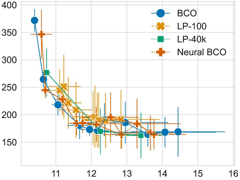
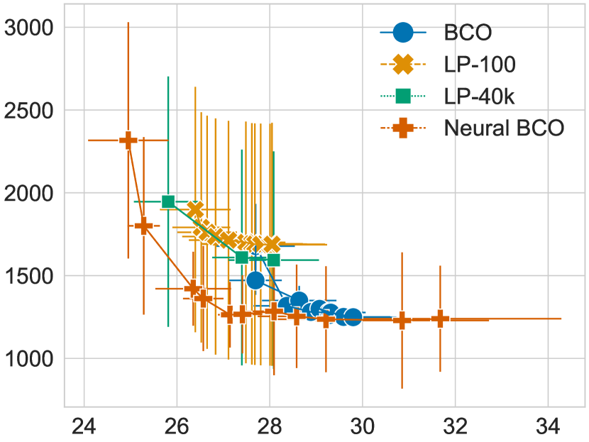
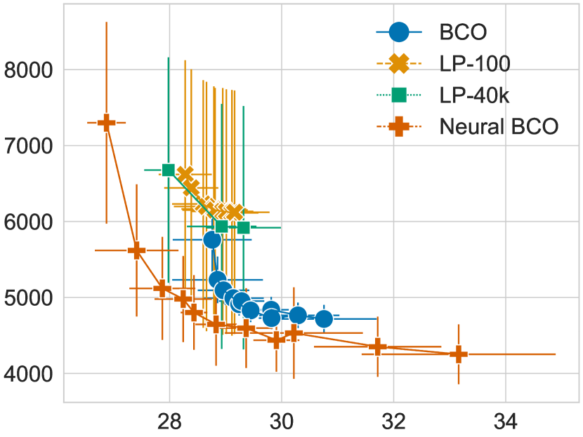
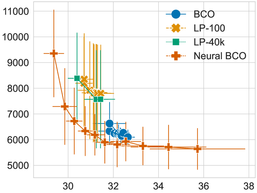
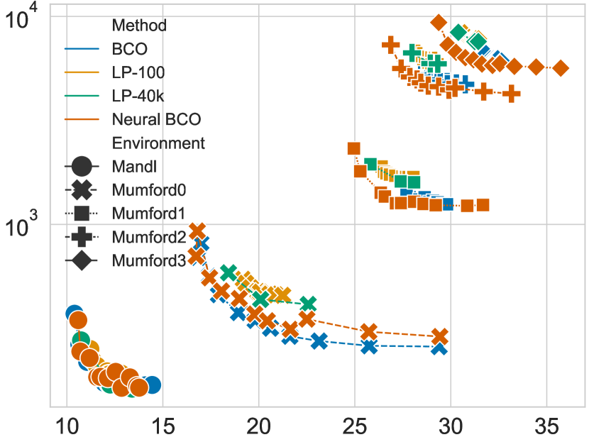
There is a necessary trade-off between minimizing the passenger cost and the operator cost : making transit routes longer increases , but allows more and faster direct connections between stops, and so may decrease . The weight can be set by the user to indicate how much they care about versus , and each algorithm output will change accordingly. Figure 1 illustrates the trade-offs made by the different methods, as we vary over its full range in steps of , except for LP-40k, for which we only plot values for and . For the two smallest cities (sub-figures 1(a) and 1(b)), BCO offers a superior trade-off for most , but for the larger cities Mumford1, 2, and 3, NBCO’s solutions not only dominate those of BCO, they achieve a much wider range of and than either of BCO or LP, which will be more satisfactory if the user cares only about one or the other component.
Both LP and BCO have more narrow ranges of and on the three larger cities, but the ranges are mostly non-overlapping. Some of NBCO’s greater range seems to be due to combining the non-overlapping ranges of the constituent parts, but NBCO’s range is greater than the union of LP’s and BCO’s ranges. This implies that the larger action space of the neural bee versus the type-1 bee allows NBCO to explore a much wider range of solutions by taking wider “steps” in solution space. Meanwhile, LP-40k has about the same range as LP-100, implying that these wide steps must be guided by the metaheuristic to eventually reach a wider space of solutions.

7 Discussion
7.1 Limitations
Bee Colony Optimization is just one instance of the broad class of metaheuristic algorithms, and while the results we present are promising, it remains to be seen whether incorporating learned heuristics into metaheuristic algorithms is a sound algorithmic strategy in general. Furthermore, in this work we consider such a combination in light of only one CO problem, the NDP. This is a very interesting and impactful problem, but evaluating this method on a wider variety of CO problems such as the TSP and VRP would more broadly establish the usefulness of this strategy.
We also note that, while the Mumford dataset is a widely used benchmark, it is still synthetic data. Establishing whether our method would be useful for transit planning in real-world cities will require evaluating on a real-world dataset.
7.2 Conclusions
Ultimately, it is doubtful whether a single-pass generation heuristic like that implemented by the GNN will be capable of outperforming search based methods like metaheuristics on combinatorial optimization problems like the NDP. By these problems’ nature, there is no one-step algorithm for finding optimal solutions, and any fast-to-compute heuristic will necessarily be approximate. Consequently, methods for exploring the solution space on a given instance have a general advantage over such heuristics. But we have shown that the choice of heuristics can have a significant impact on the quality of the solutions found by a metaheuristic, and learned heuristics in particular can significantly benefit metaheuristic algorithms when used as some of their sub-heuristics.
In terms of the applicability of these methods in real cities, we note that both LP and Neural BCO outperform BCO on all three cities - Mumford1, 2, and 3 - that were designed to match a specific real-world city in scale. Furthermore, the gap between BCO and the other methods grows with the size of the city. This suggests that Neural BCO may scale better to much larger problem sizes - which is significant, as some real-world cities have hundreds or even thousands of bus stop locations (Société de transport de Montréal, 2013).
We note that better results could likely be achieved by training a policy directly in a metaheuristic context, rather than training it in isolation and then applying it in a metaheuristic as was done here. It would also be interesting to use multiple separately-trained models as different heuristics within a metaheuristic algorithm, as opposed to the single model used in our experiments. This could be seen as a form of ensemble method, with the metaheuristic intelligently combining the strengths of the different learned models to get the best use out of each.
We would also like to explore the training of a further Machine Learning (ML) component to act as the higher-level metaheuristic, creating an entirely learned method for searching the solution space for particular problem instances. Recent work on few-shot adaptation in RL (Behbahani et al., 2023) may provide a promising starting point.
Beyond studying the relative performance of machine learning and metaheuristic approaches and their combination, we hope by this work to draw the attention of the machine community to the NDP. It is a uniquely challenging combinatorial optimization problem with real-world impact, with much potential for novel and useful study by our discipline.
References
- Ahmed et al. [2019] Leena Ahmed, Christine Mumford, and Ahmed Kheiri. Solving urban transit route design problem using selection hyper-heuristics. European Journal of Operational Research, 274(2):545–559, 2019.
- Ai et al. [2022] Guanqun Ai, Xingquan Zuo, Gang Chen, and Binglin Wu. Deep reinforcement learning based dynamic optimization of bus timetable. Applied Soft Computing, 131:109752, 2022.
- Applegate et al. [2001] David Applegate, Robert E. Bixby, Vašek Chvátal, and William J. Cook. Concorde tsp solver. https://www.math.uwaterloo.ca/tsp/concorde/index.html, 2001.
- Battaglia et al. [2018] Peter W Battaglia, Jessica B Hamrick, Victor Bapst, Alvaro Sanchez-Gonzalez, Vinicius Zambaldi, Mateusz Malinowski, Andrea Tacchetti, David Raposo, Adam Santoro, Ryan Faulkner, et al. Relational inductive biases, deep learning, and graph networks. arXiv preprint arXiv:1806.01261, 2018.
- Behbahani et al. [2023] Feryal Behbahani, Jakob Bauer, Kate Baumli, Satinder Baveja, Avishkar Bhoopchand, Nathalie Bradley-Schmieg, Michael Chang, Natalie Clay, Adrian Collister, et al. Human-timescale adaptation in an open-ended task space. arXiv preprint arXiv:2301.07608, 2023.
- Bengio et al. [2021] Yoshua Bengio, Andrea Lodi, and Antoine Prouvost. Machine learning for combinatorial optimization: a methodological tour d’horizon. European Journal of Operational Research, 290(2):405–421, 2021.
- Brody et al. [2021] Shaked Brody, Uri Alon, and Eran Yahav. How attentive are graph attention networks?, 2021. URL https://arxiv.org/abs/2105.14491.
- Bruna et al. [2013] Joan Bruna, Wojciech Zaremba, Arthur Szlam, and Yann LeCun. Spectral networks and locally connected networks on graphs. arXiv preprint arXiv:1312.6203, 2013.
- Chien et al. [2002] Steven I-Jy Chien, Yuqing Ding, and Chienhung Wei. Dynamic bus arrival time prediction with artificial neural networks. Journal of transportation engineering, 128(5):429–438, 2002.
- Dai et al. [2017] Hanjun Dai, Elias B Khalil, Yuyu Zhang, Bistra Dilkina, and Le Song. Learning combinatorial optimization algorithms over graphs. arXiv preprint arXiv:1704.01665, 2017.
- Darwish et al. [2020] Ahmed Darwish, Momen Khalil, and Karim Badawi. Optimising public bus transit networks using deep reinforcement learning. In 2020 IEEE 23rd International Conference on Intelligent Transportation Systems (ITSC), pages 1–7. IEEE, 2020.
- Defferrard et al. [2016] Michaël Defferrard, Xavier Bresson, and Pierre Vandergheynst. Convolutional neural networks on graphs with fast localized spectral filtering. CoRR, abs/1606.09375, 2016. URL http://arxiv.org/abs/1606.09375.
- Duvenaud et al. [2015] David K Duvenaud, Dougal Maclaurin, Jorge Iparraguirre, Rafael Bombarell, Timothy Hirzel, Alán Aspuru-Guzik, and Ryan P Adams. Convolutional networks on graphs for learning molecular fingerprints. Advances in neural information processing systems, 28, 2015.
- Fortune [1995] Steven Fortune. Voronoi diagrams and delaunay triangulations. Computing in Euclidean geometry, pages 225–265, 1995.
- Gilmer et al. [2017] Justin Gilmer, Samuel S. Schoenholz, Patrick F. Riley, Oriol Vinyals, and George E. Dahl. Neural message passing for quantum chemistry. In Doina Precup and Yee Whye Teh, editors, Proceedings of the 34th International Conference on Machine Learning, volume 70 of Proceedings of Machine Learning Research, pages 1263–1272. PMLR, 06–11 Aug 2017. URL https://proceedings.mlr.press/v70/gilmer17a.html.
- Guan et al. [2006] J.F. Guan, Hai Yang, and S.C. Wirasinghe. Simultaneous optimization of transit line configuration and passenger line assignment. Transportation Research Part B: Methodological, 40:885–902, 12 2006. doi: 10.1016/j.trb.2005.12.003.
- Guihaire and Hao [2008] Valérie Guihaire and Jin-Kao Hao. Transit network design and scheduling: A global review. Transportation Research Part A: Policy and Practice, 42(10):1251–1273, 2008.
- Jeong and Rilett [2004] Ranhee Jeong and R Rilett. Bus arrival time prediction using artificial neural network model. In Proceedings. The 7th international IEEE conference on intelligent transportation systems (IEEE Cat. No. 04TH8749), pages 988–993. IEEE, 2004.
- Jiang et al. [2018] Zhibin Jiang, Wei Fan, Wei Liu, Bingqin Zhu, and Jinjing Gu. Reinforcement learning approach for coordinated passenger inflow control of urban rail transit in peak hours. Transportation Research Part C: Emerging Technologies, 88:1–16, 2018. ISSN 0968-090X. doi: https://doi.org/10.1016/j.trc.2018.01.008. URL https://www.sciencedirect.com/science/article/pii/S0968090X18300111.
- John et al. [2014] Matthew P. John, Christine L. Mumford, and Rhyd Lewis. An improved multi-objective algorithm for the urban transit routing problem. In Christian Blum and Gabriela Ochoa, editors, Evolutionary Computation in Combinatorial Optimisation, pages 49–60, Berlin, Heidelberg, 2014. Springer Berlin Heidelberg. ISBN 978-3-662-44320-0.
- Kepaptsoglou and Karlaftis [2009] Konstantinos Kepaptsoglou and Matthew Karlaftis. Transit route network design problem: Review. Journal of Transportation Engineering, 135(8):491–505, 2009. doi: 10.1061/(ASCE)0733-947X(2009)135:8(491).
- Kipf and Welling [2016] Thomas N Kipf and Max Welling. Semi-supervised classification with graph convolutional networks. arXiv preprint arXiv:1609.02907, 2016.
- Kool et al. [2019] W. Kool, H. V. Hoof, and M. Welling. Attention, learn to solve routing problems! In ICLR, 2019.
- Kılıç and Gök [2014] Fatih Kılıç and Mustafa Gök. A demand based route generation algorithm for public transit network design. Computers & Operations Research, 51:21–29, 2014. ISSN 0305-0548. doi: https://doi.org/10.1016/j.cor.2014.05.001. URL https://www.sciencedirect.com/science/article/pii/S0305054814001300.
- Li et al. [2020] Can Li, Lei Bai, Wei Liu, Lina Yao, and S Travis Waller. Graph neural network for robust public transit demand prediction. IEEE Transactions on Intelligent Transportation Systems, 2020.
- Lu et al. [2019] Hao Lu, Xingwen Zhang, and Shuang Yang. A learning-based iterative method for solving vehicle routing problems. In International Conference on Learning Representations, 2019.
- Mandl [1980] Christoph E Mandl. Evaluation and optimization of urban public transportation networks. European Journal of Operational Research, 5(6):396–404, 1980.
- Mirhoseini et al. [2021] Azalia Mirhoseini, Anna Goldie, Mustafa Yazgan, Joe Wenjie Jiang, Ebrahim Songhori, Shen Wang, Young-Joon Lee, Eric Johnson, Omkar Pathak, Azade Nazi, et al. A graph placement methodology for fast chip design. Nature, 594(7862):207–212, 2021.
- Mumford [2013a] Christine L Mumford. Download link to the mumford dataset. https://users.cs.cf.ac.uk/C.L.Mumford/Research%20Topics/UTRP/CEC2013Supp.zip, 2013a. Accessed: 2023-03-24.
- Mumford [2013b] Christine L Mumford. New heuristic and evolutionary operators for the multi-objective urban transit routing problem. In 2013 IEEE congress on evolutionary computation, pages 939–946. IEEE, 2013b.
- Nikolić and Teodorović [2013] Miloš Nikolić and Dušan Teodorović. Transit network design by bee colony optimization. Expert Systems with Applications, 40(15):5945–5955, 2013.
- Quak [2003] CB Quak. Bus line planning. A passenger-oriented approach of the construction of a global line network and an efficient timetable. Master’s thesis, Delft University, Delft, Netherlands, 2003.
- Rodrigue [1997] Jean-Paul Rodrigue. Parallel modelling and neural networks: An overview for transportation/land use systems. Transportation Research Part C: Emerging Technologies, 5(5):259–271, 1997. ISSN 0968-090X. doi: https://doi.org/10.1016/S0968-090X(97)00014-4. URL https://www.sciencedirect.com/science/article/pii/S0968090X97000144.
- Société de transport de Montréal [2013] Société de transport de Montréal. Everything about the stm, 2013. URL https://web.archive.org/web/20130610123159/http://www.stm.info/english/en-bref/a-toutsurlaSTM.htm. Accessed: 2023-05-17.
- Sörensen et al. [2018] Kenneth Sörensen, Marc Sevaux, and Fred Glover. A history of metaheuristics. In Handbook of heuristics, pages 791–808. Springer, 2018.
- Sykora et al. [2020] Quinlan Sykora, Mengye Ren, and Raquel Urtasun. Multi-agent routing value iteration network. In International Conference on Machine Learning, pages 9300–9310. PMLR, 2020.
- van Nes [2003] Rob van Nes. Multiuser-class urban transit network design. Transportation Research Record, 1835(1):25–33, 2003. doi: 10.3141/1835-04. URL https://doi.org/10.3141/1835-04.
- Vaswani et al. [2017] Ashish Vaswani, Noam Shazeer, Niki Parmar, Jakob Uszkoreit, Llion Jones, Aidan N Gomez, Łukasz Kaiser, and Illia Polosukhin. Attention is all you need. In Advances in neural information processing systems, pages 5998–6008, 2017.
- Vinyals et al. [2015] Oriol Vinyals, Meire Fortunato, and Navdeep Jaitly. Pointer networks. arXiv preprint arXiv:1506.03134, 2015.
- Williams [1992] Ronald J Williams. Simple statistical gradient-following algorithms for connectionist reinforcement learning. Machine learning, 8(3):229–256, 1992.
- Xiong and Schneider [1992] Yihua Xiong and Jerry B Schneider. Transportation network design using a cumulative genetic algorithm and neural network. Transportation Research Record, 1364, 1992.
- Yan et al. [2023] Haoyang Yan, Zhiyong Cui, Xinqiang Chen, and Xiaolei Ma. Distributed multiagent deep reinforcement learning for multiline dynamic bus timetable optimization. IEEE Transactions on Industrial Informatics, 19:469–479, 2023.
- Ying et al. [2018] Rex Ying, Ruining He, Kaifeng Chen, Pong Eksombatchai, William L. Hamilton, and Jure Leskovec. Graph convolutional neural networks for web-scale recommender systems. CoRR, abs/1806.01973, 2018. URL http://arxiv.org/abs/1806.01973.
- Yoo et al. [2023] Sunhyung Yoo, Jinwoo Brian Lee, and Hoon Han. A reinforcement learning approach for bus network design and frequency setting optimisation. Public Transport, pages 1–32, 2023.
- Zou et al. [2006] Liang Zou, Jian-min Xu, and Ling-xiang Zhu. Light rail intelligent dispatching system based on reinforcement learning. In 2006 International Conference on Machine Learning and Cybernetics, pages 2493–2496, 2006. doi: 10.1109/ICMLC.2006.258785.
- Çodur and Tortum [2009] Muhammed Yasin Çodur and Ahmet Tortum. An artificial intelligent approach to traffic accident estimation: Model development and application. Transport, 24(2):135–142, 2009. doi: 10.3846/1648-4142.2009.24.135-142.
- AV
- autonomous vehicle
- TSP
- Travelling Salesman problem
- VRP
- Vehicle Routing Problem
- NDP
- Transit Network Design Problem
- FSP
- Frequency-Setting Problem
- DFSP
- Design and Frequency-Setting Problem
- SP
- Scheduling Problem
- TP
- Timetabling Problem
- NDSP
- Network Design and Scheduling Problem
- BCO
- Bee Colony Optimization
- HH
- hyperheuristic
- GA
- Genetic Algorithm
- SA
- Simulated Annealing
- MoD
- Mobility on Demand
- AMoD
- Autonomous Mobility on Demand
- IMoDP
- Intermodal Mobility-on-Demand Problem
- OD
- Origin-Destination
- CSA
- Connection Scan Algorithm
- CO
- combinatorial optimization
- NN
- neural network
- ML
- Machine Learning
- MLP
- Multi-Layer Perceptron
- RL
- Reinforcement Learning
- DRL
- Deep Reinforcement Learning
- GNN
- Graph Neural Network
- MDP
- Markov Decision Process
- DQN
- Deep Q-Networks
- ACER
- Actor-Critic with Experience Replay
- PPO
- Proximal Policy Optimization
- ARTM
- Metropolitan Regional Transportation Authority