Long time well-posedness and full justification of a Whitham-Green-Naghdi system

Abstract.

We establish the full justification of a “Whitham-Green-Naghdi”  system modeling the propagation of surface gravity waves with bathymetry in the shallow water regime. It is an asymptotic model of the water waves equations with the same dispersion relation. The model under study is a nonlocal quasilinear symmetrizable hyperbolic system without surface tension. We prove the consistency of the general water waves equations with our system at the order of precision $O(\mu^{2}({\varepsilon}+\beta))$, where $\mu$ is the shallow water parameter, ${\varepsilon}$ the nonlinearity parameter, and $\beta$ the topography parameter. Then we prove the long time well-posedness on a time scale $O(\frac{1}{\max\{{\varepsilon},\beta\}})$. Lastly, we show the convergence of the solutions of the Whitham-Green-Naghdi system to the ones of the water waves equations on the later time scale.

1. Introduction

In this article, we study a full dispersion Green-Naghdi system that describes strongly dispersive surface waves over a variable bottom. The system under consideration is described in terms of the unknowns $\zeta$, $v$, and $b$. Here $\zeta(t,x)\in{\mathbb{R}}$ denotes the surface elevation, $v(t,x)\in{\mathbb{R}}$ is related to the velocity field described by the full Euler equations, and $b$ is the elevation of the bathymetry. The system reads,

$$\begin{cases}\partial_{t}\zeta+\partial_{x}(hv)=0\\ (h+\mu h\mathcal{T}[h,\beta b])\big{(}\partial_{t}v+{\varepsilon}v\partial_{x}v\big{)}+h\partial_{x}\zeta+\mu\varepsilon h(\mathcal{Q}[h,v]+\mathcal{Q}_{b}[h,b,v])=0,\end{cases}$$ (1.1)

where $h=1+{\varepsilon}\zeta-\beta b$ and

$$\mathcal{T}[h,\beta b]v =-\frac{1}{3h}\partial_{x}\mathrm{F}^{\frac{1}{2}}\big{(}h^{3}\mathrm{F}^{\frac{1}{2}}\partial_{x}v\big{)}+\frac{1}{2h}\big{(}\partial_{x}\mathrm{F}^{\frac{1}{2}}(h^{2}(\beta\partial_{x}b)v)-h^{2}(\beta\partial_{x}b)\mathrm{F}^{\frac{1}{2}}\partial_{x}v\big{)}$$ (1.2)

$$\hskip 14.22636pt+(\beta\partial_{x}b)^{2}v,$$

and

$$\mathcal{Q}[h,v] =\frac{2}{3h}\partial_{x}\mathrm{F}^{\frac{1}{2}}\big{(}h^{3}(\mathrm{F}^{\frac{1}{2}}\partial_{x}v)^{2}\big{)}$$ (1.3)

$$\mathcal{Q}_{b}[h,\beta b,v] =h(\mathrm{F}^{\frac{1}{2}}\partial_{x}v)^{2}(\beta\partial_{x}b)+\frac{1}{2h}\partial_{x}\mathrm{F}^{\frac{1}{2}}(h^{2}v^{2}\beta\partial_{x}^{2}b)+v^{2}(\beta\partial_{x}^{2}b)(\beta\partial_{x}b),$$ (1.4)

with $\mathrm{F}^{\frac{1}{2}}$ being a Fourier multiplier associated with the dispersion relation of the water waves system. Specifically, if we let $\hat{f}(\xi)$ be the Fourier transform of $f$, then the symbol is defined in frequency by

$$\widehat{\mathrm{F}^{\frac{1}{2}}f}(\xi)=\sqrt{\frac{3}{\mu\xi^{2}}\Big{(}\frac{\sqrt{\mu}\xi}{\tanh(\sqrt{\mu}\xi)}-1\Big{)}}\hat{f}(\xi).$$ (1.5)

The parameters $\mu,{\varepsilon}$, and $\beta$ are defined by the comparison between characteristic quantities of the system under study. Among those are the characteristic water depth $H_{0}$, the characteristic wave amplitude $a_{s}$, the characteristic bathymetry amplitude $a_{b}$, and the characteristic wavelength $L$. From these comparisons appear three adimensional parameters of main importance:

• $\mu:=\frac{H_{0}^{2}}{L^{2}}$ is the shallow water parameter,

• $\varepsilon:=\frac{a_{\mathrm{s}}}{H_{0}}$ is the nonlinearity parameter,

• $\beta:=\frac{a_{b}}{H_{0}}$ is the bathymetry parameter.

Replacing the Fourier multiplier $\mathrm{F}^{\frac{1}{2}}$ by identity in system (1.1) we retrieve the classical Green-Naghdi system. The later system is proved to be consistent with the water waves equations, in the sense of Definition 5.1 in [31], at the order of precision $O(\mu^{2})$ for parameters $(\mu,\varepsilon,\beta)$ in the shallow water regime:

Definition 1.1.

Let $\mu_{\max}>0$, then we define the shallow water regime to be

$$\mathcal{A}_{\mathrm{SW}}:=\{(\mu,\varepsilon,\beta):\mu\in(0,\mu_{\max}],\varepsilon\in[0,1],\beta\in[0,1]\}.$$

Taking ${\varepsilon}$ to be zero in (1.1), we get the linearized water waves equations around the rest state with the following dispersion relation

$$\omega_{WW}(\xi)^{2}=\xi^{2}\frac{\tanh(\sqrt{\mu}\xi)}{\sqrt{\mu}\xi}.$$ (1.6)

This is why we say that system (1.1) is a full dispersion Green-Naghdi model. Moreover, it is proved in the present paper that the water waves equations are consistent, in the sense of Proposition 3.2, with system (1.1) at the order of precision $O(\mu^{2}(\varepsilon+\beta))$. The improved precision compared to the classical Green-Naghdi system allows for a change in the propagation of the waves. Such occurrences have been studied in the Dingemans experiments [7]. In these experiments, they investigated a long wave passing over a submerged obstacle. They observed that waves tend to steepen due to a compression effect from the bottom, where high harmonics generated by topography-induced nonlinear interactions are freely released behind the obstacle. This last phenomenon makes it natural that one wants to improve the frequency dispersion of the classical shallow water models. Deriving such models has been the subject of active research. Here are some references in the case of the Boussinesq model [24, 33, 5]. In the case of the Green-Naghdi model, one can consult [42] and [6], where the authors compared the classical Green-Naghdi model with one-parameter and three-parameters Green-Naghdi models in one case of the Dingemans experiments for which the propagation and interaction of highly dispersive waves are under study. By tuning the parameters, they are able to describe the dispersion relation of the water waves equations for a larger set of frequencies. As an example, the dispersion relation of the three-parameter model is

$$\omega_{GN}(\xi)^{2}=\xi^{2}\frac{(1+\mu\frac{\theta+\gamma}{3}\xi^{2})(1+\mu\frac{\alpha-1}{3}\xi^{2})}{(1+\mu\frac{\gamma}{3}\xi^{2})(1+\mu\frac{\alpha+\theta}{3}\xi^{2})},$$ (1.7)

where the parameters $\alpha,\gamma$ and $\theta$ are chosen such that (1.7) approximates well the dispersion relation of the water waves equations, (1.6), for higher frequencies. In particular, for $(\theta,\alpha,\gamma)=(-1,1,1)$ we obtain the original Green-Naghdi system. Moreover, in the case $(\theta,\alpha,\gamma)=(0.207,1,0.071)$ it was demonstrated in [6], that (1.7) is a better approximation of (1.6) (see Figure 1). This improvement allowed the authors to describe strongly dispersive waves with uneven bathymetry accurately.

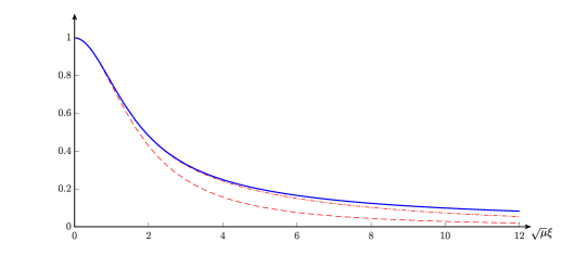
Figure 1. The blue curve is a plot of $\omega_{WW}(\xi)/\xi^{2}$ (line). The red curves plots $\omega_{GN}(\xi)/\xi^{2}$ in the case $(\theta,\alpha,\gamma)=(-1,1,1)$ (dash) and $(\theta,\alpha,\gamma)=(0.207,1,0.071)$ (dash-dots).

In fact, in the case where high frequencies are dominant, the improved Green-Naghdi models tend to describe the propagation of the waves more correctly. However, in general, one can expect to have even higher frequency interactions for which one needs to keep the full dispersion relation of the water waves equations.

The first full dispersion model, called the Whitham equations, was introduced by Whitham in [43] to study breaking waves and Stokes waves of maximal amplitude. The existence of these phenomena for this model has been proved in the recent papers [20, 25, 38, 40]. The Whitham is a classical model in oceanography and can be seen as a modified version of the Kordeweg-de Vries equations with lower frequency dispersion. In addition, the existence of periodic waves was proved in [19], and the existence of Benjamin-Feir instabilities was demonstrated in [26, 37]. See also the series of papers on the stability of traveling waves [2, 17, 29, 39],

The study of bidirectional full dispersion models for a flat bottom has also been the subject of active research. One class of such systems is the Whitham-Boussinesq ones. They are the full dispersion versions of the Boussinesq system, meaning they have the same dispersion relation as the water waves equations (1.6). Like the Whitham equation, these type of systems features solitary waves [8, 34], Benjamin-Feir instabilities [27, 35, 41], high-frequency instabilities of small-amplitude periodic traveling waves [18]. See also some comparative studies between the Boussinesq and the Whitham-Boussinesq models [4, 11].

The full dispersion Whitham-Green-Naghdi models are next order approximations of the water waves equations when compared to the Whitham-Boussinesq systems. These systems were recently derived in [21] for a flat bottom and extended to include bathymetry in [14]. See also [13] where the authors derived a two-layers Whitham-Green-Naghdi system. There is still a lot of research left to be done on the study of qualitative properties of these systems, but we mention the work of Duchene et. al [16], which proved the existence of solitary waves where they consider both surface gravity waves and internal waves.

An important part of the study of the full dispersion systems is the full justification as an asymptotic model of the water waves equations in the shallow water regime. To be more precise, we say a model is fully justified if the following points are proven:

• The solutions of the water waves equations exist on the scale $O(\frac{1}{\max\{{\varepsilon},\beta\}})$.

• The solutions of the asymptotic model exist on the scale $O(\frac{1}{\max\{{\varepsilon},\beta\}})$.

• Solutions of the water waves equations solve the asymptotic model up to remainder terms of a specified order of precision in terms of the adimensional parameters $\mu,\varepsilon$, and $\beta$. This last point is called the consistency of the water waves equations with respect to the asymptotic model.

• By virtue of the previous points, one has to show that the difference between the solutions of the water waves equations and the asymptotic model satisfies an error estimate depending polynomially on $\mu,{\varepsilon}$ and $\beta$.

If we can verify these four points, then we can compare solutions of the water waves equations with solutions of the asymptotic models up to times of order $O(\frac{1}{\max\{{\varepsilon},\beta\}})$. The first point is proved by Alvarez-Samaniego and Lannes in [1].

The three remaining points are specific to the asymptotic model. For instance, in the case of the Whitham equation, the local well-posedness in the relevant time scale follow by classical arguments on hyperbolic systems. The consistency of the water waves equations with this model has been recently proved in [22] at the order of precision $O(\mu\varepsilon)$ in the unidirectional case, but the method supposes well-prepared initial conditions. In the bidirectional case, the author proved an order of precision $O(\mu\varepsilon+\varepsilon^{2})$ and doesn’t suppose well-prepared initial conditions. In conclusion, we have the full justification of the Whitham equation at the order of precision $O(\mu\varepsilon)$ in the unidirectional case under the restriction of well-prepared initial conditions. In the bidirectional case, the order of precision is $O(\mu\varepsilon+\varepsilon^{2})$.

Regarding the Whitham-Boussinesq systems for flat bottoms, the consistency of the water waves equations with the later models has been proved in [21] with an order of precision $O(\mu\varepsilon)$ in the shallow water regime. When nonflat bottoms are considered, it has been proved in [14] to be consistent with the water waves with a precision $O(\mu({\varepsilon}+\beta))$. With respect to the second point of the justification, it has been proved for a large class of Whitham-Boussinesq systems with flat bottoms [36, 23], to be well-posed on the time scale $O(\frac{1}{{\varepsilon}})$. Lastly, we also mention earlier results on the local-well posedness on a fixed time scale given in [9, 10, 12].

For the Whitham-Green-Naghdi systems, it is proved in [21] that for a flat bottom, the water waves equations are consistent with the later systems at the order of precision $O(\mu^{2}\varepsilon)$ in the shallow water regime. Moreover, in the case of uneven bathymetry, it has been proved in [14] that the precision order is $O(\mu^{2}(\varepsilon+\beta))$. In [13], the authors proved the local well-posedness with a relevant time scale for a two-layer full dispersion Green-Naghdi model with surface tension. This system can be seen as a generalization of (1.1). However, their method relies on adding surface tension, where the time of existence tends to zero as the surface tension parameter goes to zero. Moreover, this system has only been proved to be consistent with the water waves equations at the order of precision $O(\mu^{2})$ even if, based on numerical experiments, the expected seems to be $O(\mu^{2}\varepsilon)$.

In the present paper, we prove the full justification of the Whitham-Green-Naghdi system without surface tension (1.1) as an asymptotic model of the water waves equations at the order of precision $O(\mu^{2}(\varepsilon+\beta))$.

1.1. Definition and notations

• We let $c$ denote a positive constant independent of $\mu,{\varepsilon},\beta$ that may change from line to line. Also, as a shorthand, we use the notation $a\lesssim b$ to mean $a\leq c\>b$.

• Let $s\in{\mathbb{R}}$ then the function $\lceil s\rceil$ returns the smallest integer greater than or equal to $s$.

• Let $L^{2}({\mathbb{R}})$ be the usual space of square integrable functions with norm $|f|_{L^{2}}=\sqrt{\int_{{\mathbb{R}}}|f(x)|^{2}\>dx}$. Also, for any $f,g\in L^{2}({\mathbb{R}})$ we denote the scalar product by $\big{(}f,g\big{)}_{L^{2}}=\int_{{\mathbb{R}}}f(x)\overline{g(x)}\>dx$.

• Let $f:\mathbb{R}\to\mathbb{R}$ be a tempered distribution, let $\hat{f}$ or $\mathcal{F}f$ be its Fourier transform. Let $G:\mathbb{R}\to\mathbb{R}$ be a smooth function. Then the Fourier multiplier associated with $G(\xi)$ is denoted $\mathrm{G}$ and defined by the formula:

  $$\widehat{\mathrm{G}f}(\xi)=G(\xi)\hat{f}(\xi).$$

• For any $s\in\mathbb{R}$ we call the multiplier $\widehat{\mathrm{D}^{s}f}(\xi)=|\xi|^{s}\hat{f}(\xi)$ the Riesz potential of order $-s$.

• For any $s\in\mathbb{R}$ we call the multiplier $\mathrm{J}^{s}=(1+\mathrm{D}^{2})^{\frac{s}{2}}=\langle\mathrm{D}\rangle^{s}$ the Bessel potential of order $-s$.

• The Sobolev space $H^{s}(\mathbb{R})$ is equivalent to the weighted $L^{2}-$space with $|f|_{H^{s}}=|\mathrm{J}^{s}f|_{L^{2}}$.

• For any $s\geq 1$ we will denote $\dot{H}^{s}(\mathbb{R})$ the Beppo Levi space with $|f|_{\dot{H}^{s}}=|\mathrm{J}^{s-1}\partial_{x}f|_{L^{2}}$.

• Let $k\in\mathbb{N},l\in\mathbb{N}$ and $m\in\mathbb{N}$. A function $R$ is said to be of order $O(\mu^{k}(\varepsilon^{l}+\beta^{m}))$, denoted $R=O(\mu^{k}(\varepsilon^{l}+\beta^{m})),$ if divided by $\mu^{k}(\varepsilon^{l}+\beta^{m})$ this function is uniformly bounded with respect to $(\mu,\varepsilon,\beta)\in\mathcal{A}_{\mathrm{SW}}$ in the Sobolev norms $|\cdot|_{H^{s}}$, $s\geq 0$.

• We say $f$ is a Schwartz function $\mathscr{S}(\mathbb{R})$, if $f\in C^{\infty}(\mathbb{R})$ and satisfies for all $j,k\in\mathbb{N}$,

  $$\sup\limits_{x}|x^{j}\partial_{x}^{k}f|<\infty.$$

• If $A$ and $B$ are two operators, then we denote the commutator between them to be $[A,B]=AB-BA$.

1.2. Main results

Throughout this paper, we will always make the following fundamental assumption.

Definition 1.2 (Non-cavitation assumption).

Let $s>\frac{1}{2}$, ${\varepsilon}\in(0,1)$ and $\beta\geq 0$. We say the initial surface elevation $\zeta_{0}\in H^{s}(\mathbb{R})$ and the bottom profile $b\in L^{\infty}({\mathbb{R}})$ satisfies the “non-cavitation assumption”  if there exist $h_{0}\in(0,1)$ such that

$$1+{\varepsilon}\zeta_{0}(x)-\beta b(x)\geq h_{0},\quad\text{for all}\>\>\>x\in\mathbb{R}.$$ (1.8)

Next, before we state the main results, we define the energy space associated to (1.1).

Definition 1.3.

We define the complete function space $Y^{s}_{\mu}(\mathbb{R}^{d})=H^{s}({\mathbb{R}})\times X^{s}_{\mu}({\mathbb{R}})$, where $X^{s}_{\mu}({\mathbb{R}})$ is a subspace of $H^{s+\frac{1}{2}}({\mathbb{R}})$ equipped with the norm

$$|v|_{X^{s}_{\mu}}^{2}:=|v|_{H^{s}}^{2}+\sqrt{\mu}|\mathrm{D}^{\frac{1}{2}}v|_{H^{s}}^{2},$$

and we make the definition

$$|(\zeta,v)|_{Y^{s}_{\mu}}^{2}:=|\zeta|_{H^{s}}^{2}+|v|_{X^{s}_{\mu}}^{2}.$$

The following Theorem is one of the main results of the paper and concerns the local well-posedness of (1.1) on the relevant time scale $O(\frac{1}{\max\{{\varepsilon},\beta\}})$ in the energy space.

Theorem 1.4 (Well-posedness).

Let $s>\frac{3}{2}$ and $(\mu,{\varepsilon},\beta)\in\mathcal{A}_{\mathrm{SW}}$. Assume that $(\zeta_{0},v_{0})\in Y^{s}_{\mu}(\mathbb{R})$ satisfies the non-cavitation condition (1.8) and $b\in H^{s+2}({\mathbb{R}})$. Then there exists $T=c\big{(}|(\zeta_{0},v_{0})|_{Y^{s}_{\mu}}\big{)}^{-1}$ such that (1.1) admits a unique solution

$$(\zeta,v)\in C([0,\frac{T}{\max\{{\varepsilon},\beta\}}]:Y^{s}_{\mu}(\mathbb{R}))\cap C^{1}([0,\frac{T}{\max\{{\varepsilon},\beta\}}]:Y^{s-1}_{\mu}(\mathbb{R})),$$

that satisfies

$$\sup\limits_{t\in[0,\frac{T}{\max\{{\varepsilon},\beta\}}]}|(\zeta,v)|_{Y^{s}_{\mu}}\lesssim|(\zeta_{0},v_{0})|_{Y^{s}_{\mu}}.$$ (1.9)

Furthermore, there exists a neighborhood of $(\zeta_{0},v_{0})$ such that the flow map

$$:Y_{\mu}^{s}({\mathbb{R}})\>\rightarrow\>C([0,\tfrac{T}{2\max\{{\varepsilon},\beta\}}];Y^{s}_{\mu}({\mathbb{R}})),\quad(\zeta_{0},v_{0})\>\>\mapsto\>\>(\zeta,v),$$

is continuous.

Remark 1.5.

For the sake of simplicity, we restrict our study to the one-dimensional setting. We comment on the possible extension to two dimensions at the end of Section 3.

For the next Theorem, we will state the full justification of (1.1) as a water waves model. To give the result, we first state the water waves equations:

$$\begin{cases}\partial_{t}\zeta-\frac{1}{\mu}\mathcal{G}^{\mu}[\varepsilon\zeta]\psi=0\\ \partial_{t}\psi+\zeta+\frac{\varepsilon}{2}(\partial_{x}\psi)^{2}-\frac{\mu\varepsilon}{2}\frac{(\frac{1}{\mu}\mathcal{G}^{\mu}[\varepsilon\zeta]\psi+\varepsilon\partial_{x}\zeta\cdot\partial_{x}\psi)^{2}}{1+\varepsilon^{2}\mu(\partial_{x}\zeta)^{2}}=0,\end{cases}$$ (1.10)

where $\mathcal{G}^{\mu}[\varepsilon\zeta]$ stands for the Dirichlet-Neumann operator and $\psi$ is the trace at the surface of the velocity potential $\Phi$, see [31] for more information. To compare solutions between the water waves equations and system (1.1), we define the vertical average of the horizontal component of the velocity field through the formula

$$\overline{V}=\frac{1}{h}\int_{-1+\beta b}^{\varepsilon\zeta}\partial_{x}\Phi\>\mathrm{d}z,$$ (1.11)

where $\Phi$ stands for the velocity potential in the water domain $\Omega_{t}:=\{(x,z)\in\mathbb{R}^{2},-1+\beta b\leq z\leq\varepsilon\zeta\}$. It is the solution of the following elliptic problem

$$\begin{cases}\partial_{z}^{2}\Phi+\mu\partial_{x}^{2}\Phi=0,\ \ \mathrm{in}\ \ \Omega_{t}\\ \Phi|_{z=\varepsilon\zeta}=\psi,\ \ \partial_{n}\Phi|_{z=-1+\beta b}=0,\end{cases}$$ (1.12)

where $\partial_{n}\Phi|_{z=-1+\beta b}=\partial_{z}\Phi-\mu\beta\partial_{x}b\partial_{x}\Phi$. We may now state the final result of this paper.

Theorem 1.6 (Full justification).

Let $s\in{\mathbb{N}}$ such that $s\geq 4$ and $(\mu,{\varepsilon},\beta)\in\mathcal{A}_{\mathrm{SW}}$. Then for $b\in H^{s+2}({\mathbb{R}})$ and any initial data $(\zeta_{0},\psi_{0})\in H^{s}({\mathbb{R}})\times\dot{H}^{s}({\mathbb{R}})$ satisfying the non-cavitation assumption (1.8), there exist a unique classical solution of the water waves equations (1.10) given by

$$\mathbf{U}=(\zeta,\psi)\in C([0,\frac{\tilde{T}}{\max\{{\varepsilon},\beta\}}]:H^{s}({\mathbb{R}})\times\dot{H}^{s}({\mathbb{R}})),$$

from which we define $\overline{V}\in C([0,\frac{\tilde{T}}{\max\{{\varepsilon},\beta\}}]:H^{s}({\mathbb{R}}))$ through (1.12) and (1.11).

Moreover, if we let $v_{0}^{\text{\tiny WGN}}=\overline{V}|_{t=0}$. Then $v_{0}^{\text{\tiny WGN}}\in X^{s}_{\mu}({\mathbb{R}})$ and there exist a unique classical solution, denoted by

$$\mathbf{U}^{\text{\tiny WGN}}=(\zeta^{\text{\tiny WGN}},v^{\text{\tiny WGN}})\in C([0,\frac{T}{\max\{{\varepsilon},\beta\}}]:Y^{s}_{\mu}(\mathbb{R})),$$

of the Whitham-Green-Naghdi system (1.1) sharing the same initial data

$$\mathbf{U}^{\text{\tiny WGN}}|_{t=0}=(\zeta,\overline{V})|_{t=0}.$$

Comparing the two solutions, we have that for $s\in{\mathbb{N}}$ large enough such that for all $0\leq\max\{{\varepsilon},\beta\}t\leq\min\{\tilde{T},T\}$ there holds

$$|\mathbf{U}-\mathbf{U}^{\text{\tiny WGN}}|_{L^{\infty}([0,t]\times{\mathbb{R}})}\leq C(|\zeta_{0}|_{H^{s}},|\overline{V}|_{t=0}|_{H^{s}},|b|_{H^{{s+2}}})\mu^{2}({\varepsilon}+\beta)t,$$

with $\tilde{T},T,C$ positive constants uniform with respect to $(\mu,{\varepsilon},\beta)\in\mathcal{A}_{SW}$.

Remark 1.7.

In the statement of the theorem, we simply let $s$ be large enough. The reason is due to the consistency result given by Theorem $10.5$ in [14], which links the water waves equations with a similar Whitham-Green-Naghdi system. However, it is possible to have a precise range of $s$ if one reproves this theorem and carefully tracks the “loss of derivatives”. See Section 3 for more on this point.

1.3. Outline

In Section 2, we state the technical estimates that will be used throughout the paper. In Subsection 2.1, we state some classical estimates. In Subsection 2.2 we study the properties of the Fourier multiplier $\mathrm{F}^{\frac{1}{2}}$. Lastly, in Subsection (2.3) we establish the properties related to the operator $\mathcal{T}[h,\beta b]$ defined by (1.2).

In Section 3 we prove the consistency of the water waves equations with system (1.1) at the order of precision $O(\mu^{2}(\varepsilon+\beta))$ in the shallow water regime $\mathcal{A}_{\mathrm{SW}}$. The starting point of this proof is the full dispersion Green-Naghdi system derived [14] where the precision with respect to the water waves equations (1.10) is proved to be $O(\mu^{2}(\varepsilon+\beta))$.

Sections, 4 and 5 are about establishing the energy estimates with uniform bounds on the solutions. Then as a result of the energy estimates provided in the aforementioned sections, we are in the position to prove Theorem 1.4 in Section 6. The proof relies on classical hyperbolic theory for quasilinear systems.

In Section 7, we prove the full justification result of system (1.1) resulting from all previous sections.

2. Preliminary results

2.1. Classical estimates

In this section, we state some classical results that will be used throughout the paper. First, recall the embedding results (see, for example, [32]).

Proposition 2.1 (Sobolev embedding).

Let $f\in\mathscr{S}({\mathbb{R}})$ and $s\in(0,\frac{1}{2})$. Then $H^{s}({\mathbb{R}})\hookrightarrow L^{p}({\mathbb{R}})$ with $p=\frac{2}{1-2s}$, and there holds

$$|f|_{L^{p}}\lesssim|\mathrm{D}^{s}f|_{L^{2}}.$$ (2.1)

Moreover, In the case $s>\frac{1}{2}$, then $H^{s}({\mathbb{R}})$ is continuously embedded in $L^{\infty}({\mathbb{R}})$.

Next, we state the Leibniz rule for the Riesz potential.

Proposition 2.2 (Fractional Leibniz rule [30]).

Let $\sigma=\sigma_{1}+\sigma_{2}\in(0,1)$ with $\sigma_{i}\in[0,\sigma]$ and $p,p_{1},p_{2}\in(1,\infty)$ satisfy $\frac{1}{p}=\frac{1}{p_{1}}+\frac{1}{p_{2}}$. Then, for $f,g\in\mathscr{S}({\mathbb{R}})$

$$|\mathrm{D}^{\sigma}(fg)-f\mathrm{D}^{\sigma}g-g\mathrm{D}^{\sigma}f|_{L^{p}}\lesssim|\mathrm{D}^{\sigma_{1}}f|_{L^{p_{1}}}|\mathrm{D}^{\sigma_{2}}g|_{L^{p_{2}}}.$$ (2.2)

Moreover, the case $\sigma_{2}=0$, $p_{2}=\infty$ is also allowed.

Corollary 2.3.

Let $r\in(\frac{1}{2},1)$, $f\in H^{r}({\mathbb{R}})$ and $g\in H^{\frac{1}{2}}({\mathbb{R}})$. Then

$$|fg|_{L^{2}}\lesssim|\mathrm{D}^{r-\frac{1}{2}}f|_{L^{2}}|g|_{H^{\frac{1}{2}}}$$ (2.3)

and

$$|\mathrm{D}^{\frac{1}{2}}(fg)|_{L^{2}}\lesssim|f|_{H^{r}}|g|_{H^{\frac{1}{2}}}.$$ (2.4)

Proof.

To prove (2.3), we first let $\nu\in(0,\frac{1}{2})$ to be fixed later. Then combine Hölder’s inequality with the conjugate pair $\frac{1}{p_{1}}+\frac{1}{p_{2}}=\nu+\frac{1-2\nu}{2}=\frac{1}{2}$ and (2.1) to get that

$$|fg|_{L^{2}}\lesssim|f|_{L^{\frac{1}{\nu}}}|g|_{L^{\frac{2}{1-2\nu}}}\lesssim|\mathrm{D}^{\frac{1-2\nu}{2}}f|_{L^{2}}|\mathrm{D}^{\nu}g|_{L^{2}}.$$

However, for any $r\in(\frac{1}{2},1)$ we observe that we may choose $\nu$ such that $\frac{1-2\nu}{2}=r-\frac{1}{2}$, and the proof follows.

Next, we prove (2.4). We will use Hölder’s inequality, (2.2) with $(\sigma_{1},\sigma_{2})=(\frac{1}{2},0)$, and $\frac{1}{2}=\nu+\frac{1-2\nu}{2}$ with $\nu\in(0,\frac{1}{2})$ as above to deduce

$$|\mathrm{D}^{\frac{1}{2}}(fg)|_{L^{2}} \leq|\mathrm{D}^{\frac{1}{2}}(fg)-f\mathrm{D}^{\frac{1}{2}}g-g\mathrm{D}^{\frac{1}{2}}f|_{L^{2}}+|f\mathrm{D}^{\frac{1}{2}}g|_{L^{2}}+|g\mathrm{D}^{\frac{1}{2}}f|_{L^{2}}$$

$$\lesssim|\mathrm{D}^{\frac{1}{2}}f|_{L^{\frac{1}{\nu}}}|g|_{L^{\frac{2}{1-2\nu}}}+|f|_{L^{\infty}}|\mathrm{D}^{\frac{1}{2}}g|_{L^{2}}$$

$$\lesssim|f|_{H^{r}}|g|_{H^{\frac{1}{2}}},$$

where we used (2.1) in the last line with $\frac{1-2\nu}{2}=r-\frac{1}{2}$, and the Sobolev embedding $H^{r}({\mathbb{R}})\hookrightarrow L^{\infty}({\mathbb{R}})$.

∎

Definition 2.4.

Let $d=1,2$ We say that a Fourier multiplier $\mathrm{G}(\mathrm{D})$ is of order $s$ $(s\in\mathbb{R})$ and write $\mathrm{G}\in\mathcal{S}^{s}$ if $\xi\in\mathbb{R}^{d}\mapsto G(\xi)\in\mathbb{C}$ is smooth and satisfies

$$\forall\xi\in\mathbb{R}^{d},\forall\beta\in\mathbb{N}^{d},\ \ \sup_{\xi\in\mathbb{R}^{d}}\langle\xi\rangle^{|\beta|-s}|\partial^{\beta}G(\xi)|<\infty.$$

We also introduce the seminorm

$$\mathcal{N}^{s}(\mathrm{G})=\sup_{\beta\in\mathbb{N}^{d},|\beta|\leq 2+d+\lceil\frac{d}{2}\rceil}\sup_{\xi\in\mathbb{R}^{d}}\langle\xi\rangle^{|\beta|-s}|\partial^{\beta}G(\xi)|.$$

Proposition 2.5.

Let $d=1,2$, $t_{0}>d/2$, $s\geq 0$ and $\mathrm{G}\in\mathcal{S}^{s}$. If $f\in H^{s}\cap H^{t_{0}+1}(\mathbb{R}^{d})$ then, for all $g\in H^{s-1}(\mathbb{R}^{d})$,

$$|[\mathrm{G},f]g|_{2}\leq\mathcal{N}^{s}(\mathrm{G})|f|_{H^{\max\{t_{0}+1,s\}}}|g|_{H^{s-1}}.$$ (2.5)

Proof.

See Appendix B.2 in [31] for the proof of this proposition. ∎

Next, we will need the following results to run the Bona-Smith argument (provided in the classical paper [3]) on the multiplier $\chi_{\delta}(\mathrm{D})$ defined by:

Definition 2.6.

Let $\chi\in\mathscr{S}(\mathbb{R})$ be a real valued function such that $\chi(0)=1$ and $\int_{\mathbb{R}}\chi(\xi)\mathrm{d}\xi=1$. Then for $\delta>0$ we define the regularisation operators $\mathrm{\chi}_{\delta}(\mathrm{D})$ in frequency by

$$\forall f\in L^{2}(\mathbb{R}),\quad\forall\xi\in\mathbb{R},\quad\widehat{\mathrm{\chi}_{\delta}f}(\xi):=\chi(\delta\xi)\hat{f}(\xi).$$

We give the version of the regularisation estimates as presented in [32] (Proposition $9.1$).

Proposition 2.7.

Let $s>0$, $\delta>0$ and $f\in\mathscr{S}(\mathbb{R})$. Then

$$|\chi_{\delta}(\mathrm{D})f|_{H^{s+\alpha}}\lesssim\delta^{-\alpha}|f|_{H^{s}},\quad\forall\alpha\geq 0,$$ (2.6)

and

$$|\chi_{\delta}(\mathrm{D})f-f|_{H^{s-\beta}}\lesssim\delta^{\beta}|f|_{H^{s}},\quad\forall\beta\in[0,s].$$ (2.7)

Moreover, there holds

$$|\chi_{\delta}(\mathrm{D})f-f|_{H^{s-\beta}}\underset{\delta\rightarrow 0}{=}o(\delta^{\beta}),\>\>\>\quad\forall\beta\in[0,s].$$ (2.8)

Lastly, we need an interpolation inequality. In particular, for any $s,r,t\in{\mathbb{R}}$ such that $r<t$ and $s\in(r,t)$, then for $\theta\in(0,1)$ given by $\theta+(1-\theta)=\frac{t-s}{t-r}+\frac{s-r}{t-r}$, we have by Plancherel’s identity and Hölder’s inequality that

$$|f|_{H^{s}}\leq|f|_{H^{r}}^{\theta}|f|_{H^{t}}^{(1-\theta)}.$$ (2.9)

2.2. Properties of $\mathrm{F}$

In this section, we prove estimates concerning the dispersive properties of the equation.

Proposition 2.8.

Let $s\in{\mathbb{R}}$ and $f\in\mathscr{S}({\mathbb{R}})$, then there exist $c>0$ such that

$$c^{-1}|f|_{X^{s}_{\mu}}^{2}\leq|f|_{H^{s}}^{2}+\mu|\mathrm{F}^{\frac{1}{2}}\partial_{x}f|_{H^{s}}^{2}\leq c|f|_{X^{s}_{\mu}}^{2},$$ (2.10)

$$|\mathrm{F}^{-\frac{1}{2}}f|_{H^{s}}\leq c|f|_{X_{\mu}^{s}},$$ (2.11)

$$\sqrt{\mu}|\mathrm{F}^{1}f|_{H^{s}}\leq c|f|_{H^{s-1}},$$ (2.12)

$$\mu^{\frac{1}{4}}|\mathrm{F}^{\frac{1}{2}}f|_{H^{s}}\leq c|f|_{H^{s-\frac{1}{2}}}.$$ (2.13)

Proof.

The behaviour at low frequency of the three Fourier multipliers $\mathrm{F}^{\frac{1}{2}},\mathrm{F}^{-\frac{1}{2}}$ and $\mathrm{F}^{1}$ at low frequency is

$$F^{\frac{1}{2}}(\xi),F^{-\frac{1}{2}}(\xi),F^{1}(\xi)\underset{0}{\sim}1.$$

At high frequency, their respective behavior is

$$F^{\frac{1}{2}}(\xi)\underset{\infty}{\sim}\dfrac{1}{\mu^{\frac{1}{4}}\sqrt{|\xi|}},\ \ F^{-\frac{1}{2}}(\xi)\underset{\infty}{\sim}\mu^{\frac{1}{4}}\sqrt{|\xi|},\ \ F^{1}(\xi)\underset{\infty}{\sim}\dfrac{1}{\sqrt{\mu}|\xi|}.$$

This gives us (2.11), (2.12), (2.13), and the right-hand side inequality of (2.10). It only remains to prove the left-hand side inequality of (2.10):

$$|f|_{X^{s}_{\mu}}^{2}=|f|_{H^{s}}^{2}+\sqrt{\mu}|\mathrm{D}^{\frac{1}{2}}f|_{H^{s}}^{2}$$

Now, let $\mathcal{F}(\mathbbm{1}_{\{\sqrt{\mu}|\mathrm{D}|\leq 1\}}f)(\xi)=\mathbbm{1}_{\{\sqrt{\mu}|\xi|\leq 1\}}\hat{f}(\xi)$ where $\mathbbm{1}_{\{\sqrt{\mu}|\xi|\leq 1\}}$ is the usual indicator function supported on the frequencies $\sqrt{\mu}|\xi|\leq 1$. Then we get that

$$\sqrt{\mu}|\mathrm{D}^{\frac{1}{2}}f|_{H^{s}}^{2} =\sqrt{\mu}|\mathbbm{1}_{\{\sqrt{\mu}|\mathrm{D}|\leq 1\}}\mathrm{D}^{\frac{1}{2}}\mathrm{J}^{s}f|_{L^{2}}^{2}+\sqrt{\mu}|\mathbbm{1}_{\{\sqrt{\mu}|\mathrm{D}|>1\}}\mathrm{D}^{\frac{1}{2}}\mathrm{J}^{s}f|_{L^{2}}^{2}$$

$$\lesssim\sqrt{\mu}|\mathbbm{1}_{\{\sqrt{\mu}|\mathrm{D}|\leq 1\}}\mathrm{F}^{\frac{1}{2}}\mathrm{D}^{\frac{1}{2}}\mathrm{J}^{s}f|_{L^{2}}^{2}+\mu^{\frac{3}{2}}|\mathbbm{1}_{\{\sqrt{\mu}|\mathrm{D}|>1\}}\mathrm{F}^{1}\mathrm{D}^{\frac{1}{2}}\mathrm{J}^{s}f|_{L^{2}}^{2}$$

$$\lesssim|f|_{H^{s}}^{2}+\mu|\mathrm{F}^{\frac{1}{2}}f|_{H^{s}}^{2}.$$

∎

Proposition 2.9.

Let $f,g\in\mathscr{S}({\mathbb{R}})$ and $t_{0}>\frac{1}{2}$. Then for $s\geq\frac{1}{2}$ there holds,

$$|[\mathrm{J}^{s}\mathrm{F}^{\frac{1}{2}},f]g|_{L^{2}}\lesssim|f|_{H^{\max\{t_{0}+1,s-\frac{1}{2}\}}}|\mathrm{F}^{\frac{1}{2}}g|_{H^{s-1}}.$$ (2.14)

In the case $s\geq 1$, there holds

$$|[\mathrm{J}^{s},\mathrm{F}^{\frac{1}{2}}\partial_{x}(f\cdot)]\partial_{x}g|_{L^{2}}\lesssim|\mathrm{F}^{\frac{1}{2}}\partial_{x}f|_{H^{s}}|\partial_{x}g|_{H^{t_{0}}}+|\mathrm{F}^{\frac{1}{2}}\partial_{x}g|_{H^{s}}|\partial_{x}f|_{H^{t_{0}}}.$$ (2.15)

Moreover, in the case $s=0$ we have that

$$|[\mathrm{F}^{\frac{1}{2}},f]g|_{L^{2}}\lesssim|f|_{X^{t_{0}+1}_{\mu}}|\mathrm{F}^{\frac{1}{2}}g|_{H^{-1}}.$$ (2.16)

Proof.

To prove (2.14) we note that the Fourier multiplier $\mathrm{J}^{s}\mathrm{F}^{\frac{1}{2}}$ is of order $s-\frac{1}{2}$ in the sense of Definition 2.4. Moreover, we observe that

$$\mathcal{N}^{s-\frac{1}{2}}(\mathrm{J}^{s}\mathrm{F}^{\frac{1}{2}})\lesssim\mu^{-\frac{1}{4}}.$$

Thanks to the commutator estimates of Proposition 2.5 and estimate (2.10), we have

$$|[\mathrm{J}^{s}\mathrm{F}^{\frac{1}{2}},f]g|_{L^{2}}\lesssim\mu^{-\frac{1}{4}}|f|_{H^{\max\{t_{0}+1,s-\frac{1}{2}\}}}|g|_{H^{s-\frac{3}{2}}}\lesssim|f|_{H^{\max\{t_{0}+1,s-\frac{1}{2}\}}}|\mathrm{F}^{\frac{1}{2}}g|_{H^{s-1}},$$

and proves estimate (2.14).

For the proof of (2.15), we start by estimating the bilinear form:

$$\mathrm{a}(\mathrm{D})(f,g)=[\mathrm{J}^{s},\mathrm{F}^{\frac{1}{2}}\partial_{x}(f\cdot)]\partial_{x}g,$$

given by

$$|\hat{a}(\xi)(f,g)|\leq\int_{{\mathbb{R}}}F^{\frac{1}{2}}(\xi)|\xi|\big{|}\langle\xi\rangle^{s}-\langle\rho\rangle^{s}\big{|}|\hat{f}(\xi-\rho)|\>|\widehat{\partial_{x}g}(\rho)|\>d\rho.$$

First, if $|\xi|\leq|\rho|$ we can use the mean value theorem to deduce that

$$|\hat{a}(\xi)(f,g)|\lesssim\int_{{\mathbb{R}}}F^{\frac{1}{2}}(\rho)|\rho|\langle\rho\rangle^{s-1}|\xi-\rho||\hat{f}(\xi-\rho)|\>|\widehat{\partial_{x}g}(\rho)|\>d\rho,$$

since both $\omega\mapsto\langle\omega\rangle^{s-1}$ and $\omega\mapsto F^{\frac{1}{2}}(\omega)|\omega|$ are increasing functions. By extension, we make a change of variable $\gamma=\xi-\rho$, apply Minkowski integral inequality and Cauchy-Schwarz to find the estimate

$$|[\mathrm{J}^{s},\mathrm{F}^{\frac{1}{2}}\partial_{x}(f\cdot)]\partial_{x}g|_{L^{2}} \lesssim\Big{|}\int_{{\mathbb{R}}}F^{\frac{1}{2}}(\cdot-\gamma)|\cdot-\gamma|\langle\cdot-\gamma\rangle^{s-1}|\gamma||\hat{f}(\gamma)|\>|\widehat{\partial_{x}g}(\cdot-\gamma)|\>d\gamma\Big{|}_{L^{2}_{\xi}}$$

$$\lesssim|\mathrm{F}^{\frac{1}{2}}\partial_{x}g|_{H^{s}}\int_{{\mathbb{R}}}|\gamma||\hat{f}(\gamma)|\>d\gamma$$

$$\lesssim|\mathrm{F}^{\frac{1}{2}}\partial_{x}g|_{H^{s}}|\partial_{x}f|_{H^{t_{0}}}.$$

On the other hand, when $|\rho|\leq|\xi|$ then we can argue similarly to find that

$$|\hat{a}(\xi)(f,g)| \lesssim\int_{{\mathbb{R}}}F^{\frac{1}{2}}(\xi-\rho)|\xi-\rho|\langle\xi-\rho\rangle^{s-1}|\xi-\rho||\hat{f}(\xi-\rho)|\>|\widehat{\partial_{x}g}(\rho)|\>d\rho$$

$$\hskip 14.22636pt+\int_{{\mathbb{R}}}F^{\frac{1}{2}}(\rho)|\rho|\langle\rho\rangle^{s-1}|\xi-\rho||\hat{f}(\xi-\rho)|\>|\widehat{\partial_{x}g}(\rho)|\>d\rho,$$

and as using the estimate above we conclude in this case that

$$|[\mathrm{J}^{s},\mathrm{F}^{\frac{1}{2}}\partial_{x}(f\cdot)]\partial_{x}g|_{L^{2}} \lesssim\Big{|}\int_{{\mathbb{R}}}F^{\frac{1}{2}}(\cdot-\rho)|\cdot-\rho|\langle\cdot-\rho\rangle^{s-1}|\cdot-\rho||\hat{f}(\cdot-\rho)|\>|\widehat{\partial_{x}g}(\rho)|\>d\rho\Big{|}_{L^{2}_{\xi}}$$

$$\hskip 14.22636pt+|\mathrm{F}^{\frac{1}{2}}\partial_{x}g|_{H^{s}}|\partial_{x}f|_{H^{t_{0}}}$$

$$\lesssim|\mathrm{F}^{\frac{1}{2}}\partial_{x}f|_{H^{s}}|\partial_{x}g|_{H^{t_{0}}}.+|\mathrm{F}^{\frac{1}{2}}\partial_{x}g|_{H^{s}}|\partial_{x}f|_{H^{t_{0}}}.$$

Adding the two cases completes the proof.

Next, we prove (2.16) by estimating the bilinear form:

$$|\hat{a}(\xi)(f,g)|\lesssim\int_{{\mathbb{R}}}\big{|}F^{\frac{1}{2}}(\xi)-F^{\frac{1}{2}}(\rho)\big{|}|\hat{f}(\xi-\rho)||\hat{g}(\rho)|\>d\rho.$$

Clearly, it is enough to prove that

$$k(\xi,\rho):=\big{|}F^{\frac{1}{2}}(\xi)-F^{\frac{1}{2}}(\rho)\big{|}F^{-\frac{1}{2}}(\rho)\langle\rho\rangle\lesssim 1+|\xi-\rho|F^{-\frac{1}{2}}(\xi-\rho).$$ (2.17)

Indeed, assuming the claim (2.17) and using Plancherel, Minkowski integral inequality, the Cauchy-Schwarz inequality and (2.11) we obtain the desired estimate

$$|[\mathrm{F}^{\frac{1}{2}},f]g|_{L^{2}} \leq\Big{|}\int_{{\mathbb{R}}}k(\xi,\rho)\>|\hat{f}(\xi-\rho)|\>F^{\frac{1}{2}}(\rho)\langle\rho\rangle^{-1}|\hat{g}(\rho)|\>d\rho\Big{|}_{L^{2}_{\xi}}$$

$$\lesssim\Big{|}\int_{{\mathbb{R}}}\big{(}1+|\gamma|F^{-\frac{1}{2}}(\gamma)\big{)}\>|\hat{f}(\gamma)|\>F^{\frac{1}{2}}(\xi-\gamma)\langle\xi-\gamma\rangle^{-1}|\hat{g}(\xi-\gamma)|\>d\gamma\Big{|}_{L^{2}_{\xi}}$$

$$\lesssim|f|_{X^{t_{0}+1}_{\mu}}|\mathrm{F}^{\frac{1}{2}}g|_{H^{-1}}.$$

Now, to prove the claim (2.17), we consider three cases. First, in the case $|\rho|\leq 1$ it follows directly that

$$k(\xi,\rho)\lesssim 1,$$

since $\xi\mapsto F^{\frac{1}{2}}(\xi)$ and $\rho\mapsto F^{-\frac{1}{2}}(\rho)\langle\rho\rangle$ is bounded. Next, consider the case $|\rho|>1$ and $|\xi|\leq|\rho|$. Then we note that since $\xi\mapsto F^{\frac{1}{2}}(\xi)$ is decreasing for $\xi>0$, we have the estimate

$$\frac{F(\rho)}{F(\xi)}\leq 1,$$

and moreover since $\xi\mapsto\big{(}\frac{\sqrt{\mu}\xi}{\tanh(\sqrt{\mu}\xi)}-1\big{)}$ is increasing for $\xi>0$, we get that

$$\frac{|\xi|}{|\rho|}\leq\bigg{(}\frac{|\xi|}{|\rho|}\bigg{)}^{\frac{1}{2}}\leq\bigg{(}\frac{F(\rho)}{F(\xi)}\bigg{)}^{\frac{1}{2}}\leq 1.$$ (2.18)

Thus, we obtain the bound

$$k(\xi,\rho) =\bigg{(}1-\bigg{(}\frac{F(\rho)}{F(\xi)}\bigg{)}^{\frac{1}{2}}\bigg{)}\bigg{(}\frac{F(\xi)}{F(\rho)}\bigg{)}^{\frac{1}{2}}\langle\rho\rangle$$

$$\lesssim(|\rho|-|\xi|)\bigg{(}\frac{F(\xi)}{F(\rho)}\bigg{)}^{\frac{1}{2}}.$$

Finally, to conclude this case, we make the observation that if $|\xi|\sim|\rho|$, then

$$\bigg{(}\frac{F(\xi)}{F(\rho)}\bigg{)}^{\frac{1}{2}}\lesssim 1.$$

Otherwise, we obtain

$$\bigg{(}\frac{F(\xi)}{F(\rho)}\bigg{)}^{\frac{1}{2}}\lesssim 1+\mu^{\frac{1}{4}}|\rho|^{\frac{1}{2}}\lesssim 1+\mu^{\frac{1}{4}}|\rho-\xi|^{\frac{1}{2}}.$$

Gathering these estimates allows us to conclude that

$$k(\xi,\rho)\lesssim(|\rho|-|\xi|)\bigg{(}\frac{F(\xi)}{F(\rho)}\bigg{)}^{\frac{1}{2}}\lesssim 1+|\xi-\rho|F^{-\frac{1}{2}}(\xi-\rho).$$

On the other hand, the case $|\xi|>|\rho|>1$ follows directly by changing the role of $\xi$ and $\rho$ in (2.18). Indeed, we obtain that

$$k(\xi,\rho) =\bigg{(}1-\bigg{(}\frac{F(\xi)}{F(\rho)}\bigg{)}^{\frac{1}{2}}\bigg{)}\langle\rho\rangle$$

$$\lesssim(|\xi|-|\rho|),$$

and the proof of (2.16) is complete.

∎

Proposition 2.10.

Let $s\geq 0$, and let $f\in H^{s+2}(\mathbb{R})$, then we have the following estimation on the Fourier multiplier $\mathrm{F}^{\frac{1}{2}}$

$$|(\mathrm{F}^{\frac{1}{2}}-1)f|_{H^{s}}\lesssim\mu|f|_{H^{s+2}}.$$

Proof.

First, remark that it is enough to prove the result only when $s=0$. The function defining the Fourier multiplier $\mathrm{F}^{\frac{1}{2}}$ is a smooth function on $(0,+\infty)$, continuous in $0$ with $F^{\frac{1}{2}}(0)=1$ and its first derivative is zero. Moreover, its second derivative is bounded in $[0,+\infty)$, so that from Plancherel identity and the Taylor-Lagrange formula, we get

$$|(F^{\frac{1}{2}}(\sqrt{\mu}|\xi|)-1)\hat{f}|_{2}\leq\mu||\xi|^{2}\hat{f}|_{L^{2}}.$$

In the end, we have the estimate

$$|(\mathrm{F}^{\frac{1}{2}}-1)f|_{L^{2}}\leq\mu|f|_{H^{2}}.$$

∎

2.3. Properties of $\mathscr{T}[h,\beta b]$

In this section, we study an elliptic operator associated with $\mathcal{T}[h,\beta b]$ given by (1.2). The main result is given in the following proposition where the main reference is [28].

Proposition 2.11.

Let $(\mu,{\varepsilon},\beta)\in\mathcal{A}_{\mathrm{SW}}$, $s\geq 0$, $\zeta\in H^{\max\{1,s\}}({\mathbb{R}})$, $b\in H^{s+2}({\mathbb{R}})$ and let $h=1+{\varepsilon}\zeta-\beta b$ satisfy the non-cavitation condition (1.8). Define the application

$$\mathscr{T}[h,\beta b]\>:\>\begin{cases}H^{1}({\mathbb{R}})&\rightarrow L^{2}({\mathbb{R}})\\ v&\mapsto hv+\mu h\mathcal{T}[h,\beta b]v\end{cases}$$ (2.19)

Then we have the following properties:

• The operator (2.19) is well-defined and for $v\in H^{1}({\mathbb{R}})$ there holds,

  $$|\mathscr{T}[h,\beta b]v|_{L^{2}}\lesssim|v|_{X^{\frac{1}{2}}_{\mu}}.$$ (2.20)

• The operator (2.19) is one-to-one and onto.
  

• For $s\geq 0$ and $f\in H^{s}({\mathbb{R}})$ there holds,

  $$|\mathscr{T}^{-1}[h,\beta b]f|_{X^{s}_{\mu}}\lesssim|f|_{H^{s}}.$$ (2.21)

• For $s\geq 1$ and $f\in H^{s-1}({\mathbb{R}})$ there holds,

  $$\sqrt{\mu}|\mathrm{F}^{\frac{1}{2}}\mathscr{T}^{-1}[h,\beta b]f|_{H^{s}}\lesssim|f|_{H^{s-1}}.$$ (2.22)

Proof.

We give the proof in four steps.

Step 1: The application (2.19) is well-defined. Indeed, by assumption and Sobolev embedding $H^{\frac{1}{2}^{+}}({\mathbb{R}})\hookrightarrow L^{\infty}({\mathbb{R}})$ we have that $h\in L^{\infty}({\mathbb{R}})$. Therefore, by (2.10) we get that

$$|\mathscr{T}[h,\beta b]v|_{L^{2}} \lesssim|hv|_{L^{2}}+\mu|\partial_{x}\mathrm{F}^{\frac{1}{2}}(h^{3}\mathrm{F}^{\frac{1}{2}}\partial_{x}v)|_{L^{2}}+\mu|\partial_{x}\mathrm{F}^{\frac{1}{2}}(h^{2}(\beta\partial_{x}b)v)|_{L^{2}}$$

$$\hskip 14.22636pt+\mu|h^{2}(\beta\partial_{x}b)\mathrm{F}^{\frac{1}{2}}\partial_{x}v|_{L^{2}}+\mu|h(\beta\partial_{x}b)^{2}v|_{L^{2}}$$

$$\lesssim|h|_{L^{\infty}}|v|_{L^{2}}+\mu^{\frac{3}{4}}|\mathrm{D}^{\frac{1}{2}}(h^{3}\mathrm{F}^{\frac{1}{2}}\partial_{x}v)|_{L^{2}}+\mu^{\frac{3}{4}}|\mathrm{D}^{\frac{1}{2}}(h^{2}(\beta\partial_{x}b)v)|_{L^{2}}$$

$$\hskip 14.22636pt+\mu|h^{2}(\beta\partial_{x}b)\mathrm{F}^{\frac{1}{2}}\partial_{x}v|_{L^{2}}+\mu|h|_{L^{\infty}}|(\beta\partial_{x}b)^{2}v|_{L^{2}}$$

$$=:A_{1}+A_{2}+A_{3}+A_{4}+A_{5}.$$

To conclude, we note that $(h-1)\in H^{1}({\mathbb{R}})$ and together with Hölder’s inequality, the Sobolev embedding, and (2.10) we estimate $A_{1}+A_{4}+A_{5}$:

$$A_{1}+A_{4}+A_{5}\leq c(|h-1|_{H^{1}},|h^{2}-1|_{H^{1}},\beta|\partial_{x}b|_{L^{\infty}})|v|_{X^{\frac{1}{2}}_{\mu}}.$$

The remaining terms are treated similarly, after an application of (2.4), and yield the desired estimate

$$|\mathscr{T}[h,\beta b]v|_{L^{2}}\lesssim|v|_{X^{\frac{1}{2}}_{\mu}}.$$

Step 2. The application (2.19) is one-to-one and onto. Equivalently, we prove that there exist a unique solution $v\in H^{1}({\mathbb{R}})$ to the equation

$$\mathscr{T}[h,\beta b]v=f,$$ (2.23)

for $f\in L^{2}({\mathbb{R}})$. To construct a solution, we first consider the variational formulation of (2.23) that is given by

$$a(v,\varphi)=L(\varphi),$$ (2.24)

for any $\varphi\in C^{\infty}_{c}({\mathbb{R}})$ and with

$$\begin{cases}a(v,\varphi):=\big{(}v,h\varphi\big{)}_{L^{2}}+\big{(}v,\mu h\mathcal{T}[h,\beta b]\varphi\big{)}_{L^{2}}\\ L(\varphi):=\big{(}f,\varphi\big{)}_{L^{2}}.\end{cases}$$

Then, through a direct application of the Lax-Milgram lemma, we prove there exists a unique variational solution $v\in\overline{C_{c}^{\infty}({\mathbb{R}})}^{|\cdot|_{H^{\frac{1}{2}}}}=H^{\frac{1}{2}}({\mathbb{R}})$. Indeed, we observe that the application $(u,v)\mapsto a(u,v)$ is continuous on $H^{\frac{1}{2}}({\mathbb{R}})\times H^{\frac{1}{2}}({\mathbb{R}})$:

$$|a(v,\varphi)|\leq c(|h-1|_{H^{1}},\beta|\partial_{x}b|_{L^{\infty}})|v|_{X^{0}_{\mu}}|\varphi|_{X^{0}_{\mu}},$$

by integration by parts, Hölder’s inequality and (2.10). Moreover, the coercivity estimate is deduced by first making the observation:

$$a(v,v) =\big{(}v,hv\big{)}_{L^{2}}+\mu\Big{(}h\big{(}\frac{h}{\sqrt{3}}\mathrm{F}^{\frac{1}{2}}\partial_{x}v-\frac{\sqrt{3}}{2}(\beta\partial_{x}b)v\big{)},\frac{h}{\sqrt{3}}\mathrm{F}^{\frac{1}{2}}\partial_{x}v-\frac{\sqrt{3}}{2}(\beta\partial_{x}b)v\Big{)}_{L^{2}}$$

$$\hskip 14.22636pt+\frac{\mu}{4}\big{(}h(\beta\partial_{x}b)v,(\beta\partial_{x}b)v\big{)}_{L^{2}}$$

$$\geq h_{0}|v|_{L^{2}}^{2}+\mu h_{0}\Big{|}\frac{h}{\sqrt{3}}\mathrm{F}^{\frac{1}{2}}\partial_{x}v-\frac{\sqrt{3}}{2}(\beta\partial_{x}b)v\Big{|}_{L^{2}}^{2}+\frac{\mu\beta^{2}}{4}|\sqrt{h}(\partial_{x}b)v|_{L^{2}}^{2}$$

$$=:I.$$

Now, let $\nu>0$ be chosen later and make the decomposition $I=(1-\nu)I+\nu I$. Then the first term can be bounded below by

$$(1-\nu)I\geq(1-\nu)h_{0}|v|_{L^{2}}^{2}+\frac{(1-\nu)\mu\beta^{2}}{4}|\sqrt{h}(\partial_{x}b)v|_{L^{2}}^{2}.$$

On the other hand, the remaining part is estimated by Cauchy-Schwarz and Young’s inequality:

$$\nu I \geq\frac{\nu\mu h_{0}^{3}}{3}|\mathrm{F}^{\frac{1}{2}}\partial_{x}v|_{L^{2}}^{2}-\mu\nu h_{0}\beta|\sqrt{h}|_{L^{\infty}}|\sqrt{h}(\partial_{x}b)v|_{L^{2}}|\mathrm{F}^{\frac{1}{2}}\partial_{x}v|_{L^{2}}$$

$$\geq\frac{\nu\mu h_{0}^{3}}{3}|\mathrm{F}^{\frac{1}{2}}\partial_{x}v|_{L^{2}}^{2}-\mu\nu h_{0}\Big{(}\dfrac{h_{0}^{2}}{6}|\mathrm{F}^{\frac{1}{2}}\partial_{x}v|_{L^{2}}^{2}+\dfrac{3}{2h_{0}^{2}}|\sqrt{h}|_{L^{\infty}}^{2}\beta^{2}|\sqrt{h}(\partial_{x}b)v|_{L^{2}}\Big{)}.$$

So that

$$I\geq(1-\nu)h_{0}|v|_{L^{2}}^{2}+\dfrac{\nu\mu h_{0}^{3}}{6}|\mathrm{F}^{\frac{1}{2}}\partial_{x}v|_{L^{2}}^{2}+\mu\beta^{2}\Big{(}\dfrac{1}{4}-\nu\Big{(}\dfrac{1}{4}+\dfrac{3|\sqrt{h}|_{L^{\infty}}^{2}}{2h_{0}}\Big{)}\Big{)}|\sqrt{h}(\partial_{x}b)v|_{L^{2}}.$$

Thus, to conclude, simply choose $\nu$ small enough, from which we deduce the desired estimate

$$a(v,v)\geq c|v|_{X^{0}_{\mu}}^{2}.$$ (2.25)

Lastly, the application $\varphi\mapsto L(\varphi)$ is continuous on $\varphi\in H^{\frac{1}{2}}({\mathbb{R}})$ by Cauchy-Schwarz. Consequently, we have a unique variational solution $v\in H^{\frac{1}{2}}({\mathbb{R}})$ satisfying (2.24) for any $\varphi\in H^{\frac{1}{2}}({\mathbb{R}})$. Let us show that this solution is in $H^{1}({\mathbb{R}})$, so that it also satisfies (2.23).

Let $0<\delta\leq 1$ and take $\chi_{\delta}(D)$ as in Definition 2.6 and define a sequence of smooth functions given by $v_{\delta}:=\chi_{\delta}v\in\cap_{s>0}H^{s}({\mathbb{R}})$. Then using $\mathrm{J}^{1}(\chi_{\delta})^{2}v\in H^{\frac{1}{2}}({\mathbb{R}})$ as a test function, we get

$$a(\mathrm{J}^{\frac{1}{2}}v_{\delta},\mathrm{J}^{\frac{1}{2}}v_{\delta}) =a\Big{(}v,\mathrm{J}^{1}(\chi_{\delta})^{2}v\Big{)}-\big{(}[\mathrm{J}^{\frac{1}{2}}\chi_{\delta},h]v,\mathrm{J}^{\frac{1}{2}}v_{\delta}\big{)}_{L^{2}}-\frac{\mu}{3}\big{(}[\mathrm{J}^{\frac{1}{2}}\chi_{\delta},h^{3}]\mathrm{F}^{\frac{1}{2}}\partial_{x}v,\mathrm{J}^{\frac{1}{2}}\mathrm{F}^{\frac{1}{2}}\partial_{x}v_{\delta}\big{)}_{L^{2}}$$

$$\hskip 14.22636pt+\frac{\mu}{2}\big{(}[\mathrm{J}^{\frac{1}{2}}\chi_{\delta},h^{2}(\beta\partial_{x}b)]\mathrm{F}^{\frac{1}{2}}\partial_{x}v,\mathrm{J}^{\frac{1}{2}}v_{\delta}\big{)}_{L^{2}}+\frac{\mu}{2}\big{(}[\mathrm{J}^{\frac{1}{2}}\chi_{\delta},h^{2}(\beta\partial_{x}b)]v,\mathrm{J}^{\frac{1}{2}}\mathrm{F}^{\frac{1}{2}}\partial_{x}v_{\delta}\big{)}_{L^{2}}$$

$$\hskip 14.22636pt-\mu\big{(}[\mathrm{J}^{\frac{1}{2}}\chi_{\delta},h(\beta\partial_{x}b)^{2}]v,\mathrm{J}^{\frac{1}{2}}v_{\delta}\big{)}_{L^{2}}.$$

Then using (2.24) and (2.25), we get

$$c|v_{\delta}|_{X^{\frac{1}{2}}_{\mu}}^{2} \leq a(\mathrm{J}^{\frac{1}{2}}v_{\delta},\mathrm{J}^{\frac{1}{2}}v_{\delta})$$

$$=|\big{(}f,\mathrm{J}^{1}(\chi_{\delta})^{2}v\big{)}_{L^{2}}-\big{(}[\mathrm{J}^{\frac{1}{2}}\chi_{\delta},h]v,\mathrm{J}^{\frac{1}{2}}v_{\delta}\big{)}_{L^{2}}-\frac{\mu}{3}\big{(}[\mathrm{J}^{\frac{1}{2}}\chi_{\delta},h^{3}]\mathrm{F}^{\frac{1}{2}}\partial_{x}v,\mathrm{J}^{\frac{1}{2}}\mathrm{F}^{\frac{1}{2}}\partial_{x}v_{\delta}\big{)}_{L^{2}}$$

$$\hskip 14.22636pt+\frac{\mu}{2}\big{(}[\mathrm{J}^{\frac{1}{2}}\chi_{\delta},h^{2}(\beta\partial_{x}b)]\mathrm{F}^{\frac{1}{2}}\partial_{x}v,\mathrm{J}^{\frac{1}{2}}v_{\delta}\big{)}_{L^{2}}+\frac{\mu}{2}\big{(}[\mathrm{J}^{\frac{1}{2}}\chi_{\delta},h^{2}(\beta\partial_{x}b)]v,\mathrm{J}^{\frac{1}{2}}\mathrm{F}^{\frac{1}{2}}\partial_{x}v_{\delta}\big{)}_{L^{2}}$$

$$\hskip 14.22636pt-\mu\big{(}[\mathrm{J}^{\frac{1}{2}}\chi_{\delta},h(\beta\partial_{x}b)^{2}]v,\mathrm{J}^{\frac{1}{2}}v_{\delta}\big{)}_{L^{2}}|.$$

Now remark that $\mathrm{J}^{\frac{1}{2}}\chi_{\delta}(D)$ is a Fourier multiplier of order $\frac{1}{2}$ in the sense of Definition 2.4, and that $\mathcal{N}^{\frac{1}{2}}(\mathrm{J}^{\frac{1}{2}}\chi_{\delta}(D))\lesssim 1$ uniformly in $\delta$. Hence, from Cauchy-Schwarz inequality, (2.10) and the commutator estimates of Proposition 2.5, we get

$$c|v_{\delta}|_{X^{\frac{1}{2}}_{\mu}}^{2}\leq c(|f|_{L^{2}}+|v|_{L^{2}})|v_{\delta}|_{H^{1}}.$$

We, therefore, deduce the estimate

$$\sqrt{\mu}c|v_{\delta}|_{H^{1}}\lesssim|f|_{L^{2}}+|v|_{L^{2}}.$$ (2.26)

The family $\{v_{\delta}\}_{0<\delta\leq 1}$ is uniformly bounded in $H^{1}({\mathbb{R}})$. Hence, since $H^{1}({\mathbb{R}})$ is a reflexive Banach space, there exists $V\in H^{1}({\mathbb{R}})$ and a subsequence $\{v_{\delta_{n}}\}_{0<\delta_{n}\leq 1}$ with $\delta_{n}\to 0$ such that $v_{\delta_{n}}\rightharpoonup V$. By uniqueness of the limit in $L^{2}({\mathbb{R}})$, we deduce that $v=V\in H^{1}({\mathbb{R}})$.
To conclude, we may now use (2.24) and integration by parts to find that

$$\big{(}\mathscr{T}[h,\beta b]v,\varphi\big{)}_{L^{2}}=\big{(}f,\varphi\big{)}_{L^{2}},$$

for any $\varphi\in C^{\infty}_{c}({\mathbb{R}})$. Hence, we conclude that the variational solution also provides a unique solution of (2.23).

Step 3. The estimate (2.21) holds. To prove the claim, we first consider $v$, the solution of (2.23). From the coercivity estimate (2.25) and Cauchy-Schwarz inequality, we have

$$|v|_{X^{0}_{\mu}}^{2}\lesssim a(v,v)=L(v)\leq|f|_{L^{2}}|v|_{L^{2}}\leq|f|_{L^{2}}|v|_{X^{0}_{\mu}},$$

so that

$$|v|_{X^{0}_{\mu}}\lesssim c|f|_{L^{2}}.$$ (2.27)

Next, we apply $\mathrm{J}^{s}$ to (2.23) and observe that $\mathrm{J}^{s}v$ is a distributional solution of the equation

$$\mathscr{T}[h,\beta b]v_{s} =\mathrm{J}^{s}f-[\mathrm{J}^{s},h]v+\frac{\mu}{3}\partial_{x}\mathrm{F}^{\frac{1}{2}}([\mathrm{J}^{s},h^{3}]\mathrm{F}^{\frac{1}{2}}\partial_{x}v)-\frac{\mu}{2}\partial_{x}\mathrm{F}^{\frac{1}{2}}([\mathrm{J}^{s},h^{2}(\beta\partial_{x}b)]v)$$ (2.28)

$$\hskip 14.22636pt+\frac{\mu}{2}[\mathrm{J}^{s},h^{2}(\beta\partial_{x}b)]\mathrm{F}^{\frac{1}{2}}\partial_{x}v-[\mathrm{J}^{s},h(\beta\partial_{x}b)^{2}]v$$ (2.29)

Moreover, from the coercivity estimate (2.25), the variational solution of (2.28), $v_{s}$, satisfies

$$c|v_{s}|_{X^{0}_{\mu}}^{2}\leq a(v_{s},v_{s}) =\Big{(}\mathrm{J}^{s}f-[\mathrm{J}^{s},h]v+\frac{\mu}{3}\partial_{x}\mathrm{F}^{\frac{1}{2}}([\mathrm{J}^{s},h^{3}]\mathrm{F}^{\frac{1}{2}}\partial_{x}v)-\frac{\mu}{2}\partial_{x}\mathrm{F}^{\frac{1}{2}}([\mathrm{J}^{s},h^{2}(\beta\partial_{x}b)]v)$$

$$\hskip 14.22636pt+\frac{\mu}{2}[\mathrm{J}^{s},h^{2}(\beta\partial_{x}b)]\mathrm{F}^{\frac{1}{2}}\partial_{x}v-[\mathrm{J}^{s},h(\beta\partial_{x}b)^{2}]v,v_{s}\Big{)}_{L^{2}}$$

$$=\big{(}\mathrm{J}^{s}f,v_{s})_{L^{2}}-\big{(}[\mathrm{J}^{s},h]v,v_{s}\big{)}_{L^{2}}-\frac{\mu}{3}\big{(}[\mathrm{J}^{s},h^{3}]\mathrm{F}^{\frac{1}{2}}\partial_{x}v,\mathrm{F}^{\frac{1}{2}}\partial_{x}v_{s}\big{)}_{L^{2}}$$

$$\hskip 14.22636pt+\frac{\mu}{2}\big{(}[\mathrm{J}^{s},h^{2}(\beta\partial_{x}b)]v,\mathrm{F}^{\frac{1}{2}}\partial_{x}v_{s}\big{)}_{L^{2}}+\frac{\mu}{2}\big{(}[\mathrm{J}^{s},h^{2}(\beta\partial_{x}b)]\mathrm{F}^{\frac{1}{2}}\partial_{x}v,v_{s}\big{)}_{L^{2}}$$

$$\hskip 14.22636pt-\big{(}[\mathrm{J}^{s},h(\beta\partial_{x}b)^{2}]v,v_{s}\big{)}_{L^{2}}.$$

Then using Cauchy-Schwarz inequality and the commutator estimates of Proposition 2.5, we get

$$|v_{s}|^{2}_{X^{0}_{\mu}} \lesssim c(|f|_{H^{s}}+|v|_{X^{s-1}_{\mu}})|v_{s}|_{X^{s}_{\mu}}.$$

To conclude, we first consider $s\in\mathbb{N}$ and simply argue by induction using (2.27) as a base case noting that the distributional and variational solutions must coincide, i.e. $v_{s}=\mathrm{J}^{s}v$. Then use the interpolation inequality (2.9) to obtain (2.21) for any $s$ real number $\geq 0$.

Step 4. The estimate (2.22) holds. Arguing as above, we apply $\mathrm{F}^{\frac{1}{2}}\mathrm{J}^{s}$ to (2.23) and get

$$|\mathrm{F}^{\frac{1}{2}}v|_{X^{s}_{\mu}} \lesssim a(\mathrm{F}^{\frac{1}{2}}\mathrm{J}^{s}v,\mathrm{F}^{\frac{1}{2}}\mathrm{J}^{s}v)$$

$$=\big{(}\mathrm{F}^{1}\mathrm{J}^{s}f,\mathrm{J}^{s}v)_{L^{2}}-\big{(}[\mathrm{J}^{s}\mathrm{F}^{\frac{1}{2}},h]v,\mathrm{F}^{\frac{1}{2}}\mathrm{J}^{s}v\big{)}_{L^{2}}-\frac{\mu}{3}\big{(}[\mathrm{J}^{s}\mathrm{F}^{\frac{1}{2}},h^{3}]\mathrm{F}^{\frac{1}{2}}\partial_{x}v,\mathrm{F}^{1}\partial_{x}\mathrm{J}^{s}v\big{)}_{L^{2}}$$

$$\hskip 14.22636pt+\frac{\mu}{2}\big{(}[\mathrm{J}^{s}\mathrm{F}^{\frac{1}{2}},h^{2}(\beta\partial_{x}b)]v,\mathrm{F}^{1}\partial_{x}\mathrm{J}^{s}v\big{)}_{L^{2}}+\frac{\mu}{2}\big{(}[\mathrm{J}^{s}\mathrm{F}^{\frac{1}{2}},h^{2}(\beta\partial_{x}b)]F^{\frac{1}{2}}\partial_{x}v,\mathrm{F}^{\frac{1}{2}}\mathrm{J}^{s}v\big{)}_{L^{2}}$$

$$\hskip 14.22636pt-\big{(}[\mathrm{J}^{s}\mathrm{F}^{\frac{1}{2}},h(\beta\partial_{x}b)^{2}]v,\mathrm{F}^{\frac{1}{2}}\mathrm{J}^{s}v\big{)}_{L^{2}}.$$

Now using Cauchy-Schwarz inequality, the commutator estimates (2.14) and (2.12), we get

$$|\mathrm{F}^{\frac{1}{2}}v|_{X^{s}_{\mu}}^{2} \lesssim(\frac{1}{\sqrt{\mu}}|f|_{H^{s-1}}+|v|_{H^{s-1}})|v|_{H^{s}}.$$

Moreover, for all $s\in{\mathbb{R}}$ there holds,

$$|v|_{H^{s}} \lesssim|\mathbbm{1}_{\{\sqrt{\mu}|D|\leq 1\}}v|_{H^{s}}+|\mathbbm{1}_{\{\sqrt{\mu}|D|>1\}}v|_{H^{s}}$$

$$\lesssim|\mathbbm{1}_{\{\sqrt{\mu}|D|\leq 1\}}\mathrm{F}^{\frac{1}{2}}v|_{H^{s}}+\sqrt{\mu}|\mathbbm{1}_{\{\sqrt{\mu}|D|>1\}}\mathrm{F}^{1}\partial_{x}v|_{H^{s}}$$

$$\lesssim|\mathrm{F}^{\frac{1}{2}}v|_{H^{s}}+\sqrt{\mu}|\mathrm{F}^{1}\partial_{x}v|_{H^{s}}$$

$$\lesssim|\mathrm{F}^{\frac{1}{2}}v|_{X^{s}_{\mu}}.$$

Thus, by gathering these estimates we get

$$\sqrt{\mu}|\mathrm{F}^{\frac{1}{2}}v|_{X^{s}_{\mu}}\lesssim c\big{(}|f|_{H^{s-1}}+\sqrt{\mu}|\mathrm{F}^{\frac{1}{2}}v|_{X^{s-1}_{\mu}}\big{)},$$

and allows us to argue by induction for $s\in\mathbb{N}\backslash\{0\}$, where the base case reads

$$|\mathrm{F}^{\frac{1}{2}}v|_{X^{0}_{\mu}}\lesssim|v|_{X^{0}_{\mu}}\lesssim|f|_{L^{2}}$$

Then use (2.9) to conclude the proof. In the end, we have the estimate

$$\sqrt{\mu}|\mathrm{F}^{\frac{1}{2}}v|_{H^{s}}\leq\sqrt{\mu}|\mathrm{F}^{\frac{1}{2}}v|_{X^{s}_{\mu}}\leq c|f|_{H^{s-1}}.$$

∎

3. Consistency between (1.1) and (1.10)

To derive system (1.1), we start from the full dispersion Green-Naghdi model derived in [14] for which we know the order of precision with respect to the water waves equations (1.10).

Proposition 3.1 (Theorem $10.5$ in [14]).

There exists $n\in\mathbb{N}$ and $T>0$ such that for all $s\geq 0$ and $(\mu,\varepsilon,\beta)\in\mathcal{A}_{\mathrm{SW}}$, with $b\in H^{s+n}({\mathbb{R}})$ and for every solution $(\zeta,\psi)\in C([0,\frac{T}{\varepsilon}];H^{s+n}(\mathbb{R})\times\dot{H}^{s+n}(\mathbb{R}))$ to the water waves equations (1.10) one has

$$\begin{cases}\partial_{t}\zeta+\partial_{x}(h\overline{V})=0\\ \partial_{t}(\overline{V}+\mu\mathcal{T}[h,\beta\partial_{x}b]\overline{V})+\partial_{x}\zeta+{\varepsilon}\overline{V}\partial_{x}\overline{V}+\mu{\varepsilon}\partial_{x}\mathcal{R}[h,\beta\partial_{x}b,\overline{V}]=\mu^{2}(\varepsilon+\beta)R,\end{cases}$$ (3.1)

where $\overline{V}$ is defined through (1.12) and (1.11), and

$$\mathcal{T}[h,\beta b]\overline{V} =-\frac{1}{3h}\partial_{x}\mathrm{F}^{\frac{1}{2}}(h^{3}\mathrm{F}^{\frac{1}{2}}\partial_{x}\overline{V})+\frac{1}{2h}\Big{(}\partial_{x}\mathrm{F}^{\frac{1}{2}}(h^{2}(\beta\partial_{x}b)\overline{V})-h^{2}(\beta\partial_{x}b)\mathrm{F}^{\frac{1}{2}}\partial_{x}\overline{V}\Big{)}$$

$$\hskip 284.52756pt+(\beta\partial_{x}b)^{2}\overline{V},$$

$$\mathcal{R}[h,\beta b,\overline{V}] =-\frac{\overline{V}}{3h}\partial_{x}\mathrm{F}^{\frac{1}{2}}\big{(}h^{3}\mathrm{F}^{\frac{1}{2}}\partial_{x}\overline{V}\big{)}-\frac{1}{2}h^{2}\big{(}\mathrm{F}^{\frac{1}{2}}\partial_{x}\overline{V}\big{)}^{2}$$

$$\hskip 56.9055pt+\frac{1}{2}\Big{(}\frac{\overline{V}}{h}\partial_{x}\mathrm{F}^{\frac{1}{2}}\big{(}h^{2}(\beta\partial_{x}b)\overline{V}\big{)}+h(\beta\partial_{x}b)\overline{V}\mathrm{F}^{\frac{1}{2}}\partial_{x}\overline{V}+(\beta\partial_{x}b)^{2}\overline{V}^{2}\Big{)},$$

and where $|R|_{H^{s}}\leq C(\frac{1}{h_{0}},\mu_{\max},|\zeta|_{H^{s+n)}},|\partial_{x}\psi|_{H^{s+n}},|b|_{H^{s+n}})$.

Furthermore, we say that the water waves equations are consistent with the system (3.1) at the order of precision $O(\mu^{2}(\varepsilon+\beta))$ in the shallow water regime.

Proposition 3.2.

The water waves equations are consistent with the system

$$\begin{cases}\partial_{t}\zeta+\partial_{x}(h\overline{V})=0\\ (h+\mu h\mathcal{T}[h,\beta\partial_{x}b])\big{(}\partial_{t}\overline{V}+{\varepsilon}\overline{V}\partial_{x}\overline{V}\big{)}+h\partial_{x}\zeta+\mu\varepsilon h(\mathcal{Q}[h,\overline{V}]+\mathcal{Q}_{b}[h,b,\overline{V}])=0,\end{cases}$$

at the order of precision $O(\mu^{2}(\varepsilon+\beta))$, where

$$\mathcal{Q}[h,\overline{V}] =\frac{2}{3h}\partial_{x}\mathrm{F}^{\frac{1}{2}}\big{(}h^{3}(\mathrm{F}^{\frac{1}{2}}\partial_{x}\overline{V})^{2}\big{)}$$ (3.2)

$$\mathcal{Q}_{b}[h,\beta b,\overline{V}] =h(\mathrm{F}^{\frac{1}{2}}\partial_{x}\overline{V})^{2}(\beta\partial_{x}b)+\frac{1}{2h}\partial_{x}\mathrm{F}^{\frac{1}{2}}(h^{2}\overline{V}^{2}\beta\partial_{x}^{2}b)+\overline{V}^{2}(\beta\partial_{x}^{2}b)(\beta\partial_{x}b).$$ (3.3)

Proof.

Let us first remark that we only have to work on the second equation of system (3.1) and that the first equation can also be written

$$\partial_{t}h=-\varepsilon\partial_{x}(h\overline{V}).$$ (3.4)

Then multiplying the second equation of (3.1) by $h$ we can write

$$h\partial_{t}\big{(}\overline{V}+\mu\mathcal{T}[h,\beta b]\overline{V}\big{)}=(h+\mu h\mathcal{T}[h,\beta b])\partial_{t}\overline{V}+h[\partial_{t},\mu\mathcal{T}[h,\beta b]]\overline{V}.$$

Now, using (3.4) we observe that the following terms are of order $\mu{\varepsilon}$:

$$h[\partial_{t},\mu\mathcal{T}[h,\beta b]]\overline{V}+\mu\varepsilon h\mathcal{R}[h,v],$$

and so we can use Proposition 2.10 to trade the multiplier $\mathrm{F}^{\frac{1}{2}}$ with identity and terms of order $\mu^{2}{\varepsilon}$. Thus, following the derivation presented in [28] we obtain that

$$(h+\mu h\mathcal{T}[h,\beta\partial_{x}b])\big{(}\partial_{t}\overline{V}+{\varepsilon}\overline{V}\partial_{x}\overline{V}\big{)}+h\partial_{x}\zeta+\mu\varepsilon h(\tilde{\mathcal{Q}}[h,\overline{V}]+\tilde{\mathcal{Q}}_{b}[h,b,\overline{V}])=O(\mu^{2}{\varepsilon})$$

where

$$\tilde{\mathcal{Q}}[h,\overline{V}] =\frac{2}{3h}\partial_{x}\big{(}h^{3}(\partial_{x}\overline{V})^{2}\big{)}$$

$$\tilde{\mathcal{Q}}_{b}[h,\beta b,\overline{V}] =h(\partial_{x}\overline{V})^{2}(\beta\partial_{x}b)+\frac{1}{2h}\partial_{x}(h^{2}\overline{V}^{2}\beta\partial_{x}^{2}b)+\overline{V}^{2}(\beta\partial_{x}^{2}b)(\beta\partial_{x}b).$$

To conclude, we simply apply Proposition 2.10 once more to see that

$$\tilde{\mathcal{Q}}[h,\overline{V}]=\mathcal{Q}[h,\overline{V}]+O(\mu)$$

and

$$\tilde{\mathcal{Q}}_{b}[h,\beta b,\overline{V}]=\mathcal{Q}_{b}[h,\beta b,\overline{V}]+O(\mu).$$

∎

Remark 3.3.

If we consider the two-dimensional case where we let $X=(x_{1},x_{2})$ and $\overline{V},R\in{\mathbb{R}}^{2}$, then system (3.1) reads

$$\begin{cases}\partial_{t}\zeta+\nabla_{X}\cdot(h\overline{V})=0\\ \partial_{t}(\overline{V}+\mu\mathcal{T}[h,\beta b]\overline{V})+\nabla_{X}\zeta+\frac{{\varepsilon}}{2}\nabla_{X}|\overline{V}|^{2}+\mu{\varepsilon}\nabla_{X}\mathcal{R}[h,\beta\partial_{x}b,\overline{V}]=\mu^{2}(\varepsilon+\beta)R.\end{cases}$$ (3.5)

In this case, one can exploit the observation that the quantity

$$U=\overline{V}+\mu\mathcal{T}[h,\beta b]\overline{V}$$ (3.6)

approximates the gradient of the velocity potential at the free surface. Consequently, for regular solutions, one can impose the condition $\mathrm{curl}\>U|_{t=0}=0$ and using the second equation in (3.5), we can deduce that $\mathrm{curl}\>U=0$ whenever the solution is defined. However, this observation does not carry over to (1.1) since the two systems are not equivalent. On the other hand, if $\mathrm{F}=\mathrm{Id}$, then the two systems are equivalent, and one may exploit this insight to deal with the two-dimensional case.

Remark 3.4.

The estimates in Section $2$ can be extended to two dimensions where we note that $F^{\frac{1}{2}}(\xi)$ is a radial function. Also, in light of the previous remark, it could be possible to work on system (3.5) directly where we estimate the variables $\zeta$, $U$ and with $\overline{V}=\overline{V}[h,\beta b,U]$ uniquely defined by (3.6) (see [15] for similar observations). However, doing this change of unknowns would change the mathematical structure of the equations. So that it is not obvious that we can close the energy method in that case.

4. A priori estimates

In this section, we establish a priori bounds on the solutions of (1.1). To this end, we let $\mathbf{U}=(\zeta,v)$ and for simplicity we introduce the notation

$$\mathscr{T}=\mathscr{T}[h,\beta b],\quad\mathcal{Q}=\mathcal{Q}[h,v],\quad\mathcal{Q}_{b}=\mathcal{Q}_{b}[h,\beta b,v],$$

allowing us to write (1.1) on the more compact form:

$$S(\mathbf{U})(\partial_{t}\mathbf{U}+M_{1}(\mathbf{U})\partial_{x}\mathbf{U})+M_{2}(\mathbf{U})\partial_{x}\mathbf{U}+Q(\mathbf{U})+Q_{b}(\mathbf{U})=\mathbf{0},$$ (4.1)

with

$$S(\mathbf{U}):=\begin{pmatrix}1&0\\ 0&\mathscr{T}(\cdot)\end{pmatrix},\quad M_{1}(\mathbf{U}):=\begin{pmatrix}0&0\\ 0&{\varepsilon}v\end{pmatrix},\quad M_{2}(\mathbf{U}):=\begin{pmatrix}{\varepsilon}v&h\\ h&0\end{pmatrix},$$

and where the quadratic terms are

$$Q(\mathbf{U})=\begin{pmatrix}0\\ \mu{\varepsilon}h\mathcal{Q}\end{pmatrix},\quad Q_{b}(\mathbf{U})=\begin{pmatrix}-(\beta\partial_{x}b)v\\ \mu{\varepsilon}h\mathcal{Q}_{b}\end{pmatrix},$$ (4.2)

with $\mathcal{Q}$ as defined by (1.3) and $\mathcal{Q}_{b}$ defined by (1.4). We may now give the energy and the energy estimate of (4.1). In particular, we make the definition:

$$E_{s}(\mathbf{U})=\big{(}\mathrm{J}^{s}\mathbf{U},S(\mathbf{U})\mathrm{J}^{s}\mathbf{U}\big{)}_{L^{2}},$$ (4.3)

allowing us to state the following result.

Proposition 4.1.

Let $s>\frac{3}{2}$, $(\mu,{\varepsilon},\beta)\in\mathcal{A}_{SW}$, and $(\zeta,v)\in C([0,T];Y^{s}_{\mu}(\mathbb{R}))$ be a solution to (4.1) on a time interval $[0,T]$ for some $T>0$. Moreover, assume $b\in H^{s+2}({\mathbb{R}})$ and there exist $h_{0}\in(0,1)$ such that

$$h_{0}-1+\beta b\leq{\varepsilon}\zeta(x,t),\quad\forall(x,t)\in\mathbb{R}\times[0,T],$$ (4.4)

and suppose that

$$N(s):={\varepsilon}\sup\limits_{t\in[0,T]}|(\zeta(t,\cdot),v(t,\cdot))|_{Y^{s}_{\mu}}+\beta|b|_{H^{s+2}}\leq N^{\star},$$ (4.5)

for some $N^{\star}\in{\mathbb{R}}^{+}$. Then, for the energy given by (4.3), there holds,

$$\frac{d}{dt}E_{s}(\mathbf{U})\lesssim N(s)E_{s}(\mathbf{U}),$$ (4.6)

and

$$|(\zeta,v)|^{2}_{Y^{s}_{\mu}}\lesssim E_{s}(\mathbf{U})\lesssim|(\zeta,v)|^{2}_{Y^{s}_{\mu}},$$ (4.7)

for all $0<t<T$.

Proof.

We first prove (4.7). We note that the energy is similar to the bilinear form defined in (2.24). Thus, the estimate is a direct consequence of Step 2. in the proof of Proposition 2.11 and (4.4).

Next, we prove (4.6). Using (4.1), the self-adjointness of $S(\mathbf{U})$ and the invertibility provided by Proposition 2.11 under assumption (4.4), we obtain that

$$\frac{1}{2}\frac{d}{dt}E_{s}(\mathbf{U}) =\frac{1}{2}\big{(}\mathrm{J}^{s}\mathbf{U},(\partial_{t}S(\mathbf{U}))\mathrm{J}^{s}\mathbf{U}\big{)}_{L^{2}}+\big{(}\mathrm{J}^{s}\partial_{t}\mathbf{U},S(\mathbf{U})\mathrm{J}^{s}\mathbf{U}\big{)}_{L^{2}}$$

$$=\frac{1}{2}\big{(}\mathrm{J}^{s}\mathbf{U},(\partial_{t}S(\mathbf{U}))\mathrm{J}^{s}\mathbf{U}\big{)}_{L^{2}}-\big{(}\mathrm{J}^{s}M_{1}(\mathbf{U})\partial_{x}\mathbf{U},S(\mathbf{U})\mathrm{J}^{s}\mathbf{U}\big{)}_{L^{2}}$$

$$\hskip 14.22636pt-\big{(}M_{2}(\mathbf{U})\partial_{x}\mathrm{J}^{s}\mathbf{U},\mathrm{J}^{s}\mathbf{U}\big{)}_{L^{2}}-\big{(}[\mathrm{J}^{s},(S^{-1}M_{2})(\mathbf{U})]\partial_{x}\mathbf{U},S(\mathbf{U})\mathrm{J}^{s}\mathbf{U}\big{)}_{L^{2}}$$

$$\hskip 14.22636pt-\big{(}\mathrm{J}^{s}(S^{-1}Q)(\mathbf{U}),S(\mathbf{U})\mathrm{J}^{s}\mathbf{U}\big{)}_{L^{2}}-\big{(}\mathrm{J}^{s}(S^{-1}Q_{b})(\mathbf{U}),S(\mathbf{U})\mathrm{J}^{s}\mathbf{U}\big{)}_{L^{2}}$$

$$=:I+II+III+IV+V+VI.$$

Control of $I$. We first use the equation for $\partial_{t}\zeta$ in (4.1), together with the Sobolev embedding $H^{s-1}(\mathbb{R})\hookrightarrow L^{\infty}({\mathbb{R}})$ with $s-1>\frac{1}{2}$ and the algebra property to deduce the estimate:

$$|\partial_{t}h|_{L^{\infty}} \leq{\varepsilon}|\partial_{x}(hv)|_{L^{\infty}}$$

$$\lesssim{\varepsilon}(1+{\varepsilon}|\zeta|_{H^{s}}+\beta|b|_{H^{s}})|v|_{H^{s}}.$$ (4.8)

Therefore, by definition (2.19) of $\mathscr{T}[h,\beta b]$, using integration by parts, Hölder’s inequality, (4.5), Sobolev embedding, and (4.7) we obtain the bound

$$|I| \leq\frac{1}{2}|\big{(}\mathrm{J}^{s}v,(\partial_{t}h)\mathrm{J}^{s}v\big{)}_{L^{2}}|+\frac{\mu}{6}|\big{(}\mathrm{F}^{\frac{1}{2}}\partial_{x}\mathrm{J}^{s}v,(\partial_{t}(h^{3}))\mathrm{F}^{\frac{1}{2}}\partial_{x}\mathrm{J}^{s}v\big{)}_{L^{2}}|$$

$$\hskip 14.22636pt+\frac{\mu}{2}|\big{(}\mathrm{F}^{\frac{1}{2}}\partial_{x}\mathrm{J}^{s}v,(\partial_{t}(h^{2}))\beta(\partial_{x}b)\mathrm{J}^{s}v\big{)}_{L^{2}}|+\mu|\big{(}\mathrm{J}^{s}v,(\partial_{t}h)(\beta\partial_{x}b)^{2}\mathrm{J}^{s}v\big{)}_{L^{2}}|$$

$$\lesssim N(s)E_{s}(\mathbf{U}),$$

for $s>\frac{3}{2}$.

Control of $II$. By definition of $\mathscr{T}[h,\beta b]$ we must deal with the terms:

$$II =-{\varepsilon}\big{(}\mathrm{J}^{s}(v\partial_{x}v),h\mathrm{J}^{s}v\big{)}_{L^{2}}+\frac{\mu{\varepsilon}}{3}\big{(}\mathrm{J}^{s}(v\partial_{x}v),\partial_{x}\mathrm{F}^{\frac{1}{2}}(h^{3}\partial_{x}\mathrm{F}^{\frac{1}{2}}\mathrm{J}^{s}v)\big{)}_{L^{2}}$$

$$\hskip 14.22636pt-\frac{\mu{\varepsilon}\beta}{2}\big{(}\mathrm{J}^{s}(v\partial_{x}v),\partial_{x}\mathrm{F}^{\frac{1}{2}}(h^{2}(\partial_{x}b)\mathrm{J}^{s}v)\big{)}_{L^{2}}+\frac{\mu{\varepsilon}\beta}{2}\big{(}\mathrm{J}^{s}(v\partial_{x}v),h^{2}(\partial_{x}b)\partial_{x}\mathrm{F}^{\frac{1}{2}}\mathrm{J}^{s}v\big{)}_{L^{2}}$$

$$\hskip 14.22636pt-\frac{\mu{\varepsilon}\beta}{2}\big{(}\mathrm{J}^{s}(v\partial_{x}v),h(\beta\partial_{x}b)^{2}\mathrm{J}^{s}v\big{)}_{L^{2}}$$

$$=:II_{1}+II_{2}+II_{3}+II_{4}+II_{5}.$$

Using integration by parts, we may decompose $II_{1}$ into two pieces

$$II_{1} =-{\varepsilon}\big{(}hv\mathrm{J}^{s}\partial_{x}v,\mathrm{J}^{s}v\big{)}_{L^{2}}-{\varepsilon}\big{(}[\mathrm{J}^{s},v]\partial_{x}v,h\mathrm{J}^{s}v\big{)}_{L^{2}}$$

$$=\frac{{\varepsilon}}{2}\big{(}(\partial_{x}(hv))\mathrm{J}^{s}v,\mathrm{J}^{s}v\big{)}_{L^{2}}-{\varepsilon}\big{(}[\mathrm{J}^{s},v]\partial_{x}v,h\mathrm{J}^{s}v\big{)}_{L^{2}}.$$

Then by Hölder’s inequality, Sobolev embedding, and the commutator estimate (2.5), we obtain the estimate:

$$|II_{1}|\lesssim{\varepsilon}(1+|h-1|_{H^{s}})|v|_{H^{s}}^{3}.$$

We also note that $II_{5}$ can be estimated in the same way, and we obtain easily that

$$|II_{5}|\lesssim{\varepsilon}(1+|h-1|_{H^{s}})|b|_{H^{s+1}}^{2}|v|_{H^{s}}^{3}.$$

For $II_{2}$, we also use integration by parts to make the observation:

$$II_{2} =-\frac{\mu{\varepsilon}}{3}\big{(}[\mathrm{J}^{s},\mathrm{F}^{\frac{1}{2}}\partial_{x}(v\cdot)]\partial_{x}v,h^{3}\partial_{x}\mathrm{F}^{\frac{1}{2}}\mathrm{J}^{s}v\big{)}_{L^{2}}-\frac{\mu{\varepsilon}}{3}\big{(}\mathrm{F}^{\frac{1}{2}}\partial_{x}(v\mathrm{J}^{s}\partial_{x}v),h^{3}\partial_{x}\mathrm{F}^{\frac{1}{2}}\mathrm{J}^{s}v\big{)}_{L^{2}}$$

$$=:II_{2}^{1}+II_{2}^{2}.$$

Then we treat $II_{2}^{1}$ with Hölder’s inequality, Sobolev embedding, and (2.15) to get

$$|II_{2}^{1}| \lesssim(1+|h^{3}-1|_{H^{s}})|v|_{H^{s}}|v|_{X^{s}_{\mu}}^{2}.$$

On the other hand, we need to decompose $II_{2}^{2}$ further and carefully distribute the $\mu$:

$$II_{2}^{2} =-\frac{\mu{\varepsilon}}{3}\big{(}v\mathrm{F}^{\frac{1}{2}}\mathrm{J}^{s}\partial_{x}^{2}v,h^{3}\partial_{x}\mathrm{F}^{\frac{1}{2}}\mathrm{J}^{s}v\big{)}_{L^{2}}-\frac{\mu{\varepsilon}}{3}\big{(}[\mathrm{F}^{\frac{1}{2}},v]\mathrm{J}^{s}\partial_{x}^{2}v,h^{3}\partial_{x}\mathrm{F}^{\frac{1}{2}}\mathrm{J}^{s}v\big{)}_{L^{2}}$$

$$\hskip 14.22636pt-\frac{\mu{\varepsilon}}{3}\big{(}\mathrm{F}^{\frac{1}{2}}\big{(}(\partial_{x}v)\mathrm{J}^{s}\partial_{x}v\big{)},h^{3}\partial_{x}\mathrm{F}^{\frac{1}{2}}\mathrm{J}^{s}v\big{)}_{L^{2}}$$

$$=:II_{2}^{2,1}+II_{2}^{2,2}+II_{2}^{2,3}.$$

For $II_{2}^{2,1}$, we simply integrate by parts and argue as we did for $II_{1}$ to obtain

$$|II_{2}^{2,1}| \lesssim\mu{\varepsilon}|\partial_{x}(h^{3}v)|_{H^{s-1}}|\mathrm{F}^{\frac{1}{2}}\mathrm{J}^{s}\partial_{x}v|_{H^{s}}^{2}$$

$$\lesssim{\varepsilon}(1+|h^{3}-1|_{H^{s}})|v|_{H^{s}}|v|_{X_{\mu}^{s}}^{2}.$$

For $II_{2}^{2,2}$, we use Hölder’s inequality, Sobolev embedding, and (2.16) to directly obtain that

$$|II_{2}^{2,2}| \lesssim\mu{\varepsilon}(1+|h^{3}-1|_{H^{s}})|v|_{X^{s}_{\mu}}|\mathrm{F}^{\frac{1}{2}}\partial_{x}^{2}v|_{H^{s-1}}|\mathrm{F}^{\frac{1}{2}}\partial_{x}v|_{H^{s}}$$

$$\lesssim{\varepsilon}(1+|h^{3}-1|_{H^{s}})|v|_{X^{s}_{\mu}}^{3}.$$

For $II_{2}^{2,3}$, we also need to be careful in the distribution of $\mu$. In fact, we need to use Plancherel, then Cauchy-Schwarz and (2.11) to get

$$|II_{2}^{2,3}| =\frac{\mu{\varepsilon}}{3}|\big{(}\mathrm{F}^{\frac{1}{2}}\mathrm{J}^{s}\partial_{x}v,\mathrm{F}^{-\frac{1}{2}}\Big{(}(\partial_{x}v)\mathrm{F}^{\frac{1}{2}}\big{(}h^{3}\partial_{x}\mathrm{F}^{\frac{1}{2}}\mathrm{J}^{s}v\big{)}\Big{)}\big{)}_{L^{2}}|$$

$$\lesssim{\varepsilon}|v|_{X^{s}_{\mu}}\big{(}\sqrt{\mu}|(\partial_{x}v)\mathrm{F}^{\frac{1}{2}}\big{(}h^{3}\partial_{x}\mathrm{F}^{\frac{1}{2}}\mathrm{J}^{s}v\big{)}|_{L^{2}}+\mu^{\frac{3}{4}}|\mathrm{D}^{\frac{1}{2}}\Big{(}(\partial_{x}v)\mathrm{F}^{\frac{1}{2}}\big{(}h^{3}\partial_{x}\mathrm{F}^{\frac{1}{2}}\mathrm{J}^{s}v\big{)}\Big{)}|_{L^{2}}\big{)}$$

$$=:{\varepsilon}|v|_{X^{s}_{\mu}}(A+B).$$

Then estimate $A$ by Hölder’s inequality, the Sobolev embedding, and the boundedness of $\mathrm{F}^{\frac{1}{2}}$ on $L^{2}({\mathbb{R}})$ to get

$$A\lesssim|v|_{H^{s}}(1+|h^{3}-1|_{H^{s}})|v|_{X^{s}_{\mu}},$$

while for $B$, we also use (2.4) and (2.13) to get

$$B \lesssim\mu^{\frac{3}{4}}|v|_{H^{s}}|\mathrm{F}^{\frac{1}{2}}\big{(}h^{3}\partial_{x}\mathrm{F}^{\frac{1}{2}}\mathrm{J}^{s}v\big{)}|_{H^{\frac{1}{2}}}$$

$$\lesssim\sqrt{\mu}|v|_{H^{s}}|h^{3}\partial_{x}\mathrm{F}^{\frac{1}{2}}\mathrm{J}^{s}v|_{L^{2}}$$

$$\lesssim|v|_{H^{s}}(1+|h^{3}-1|_{H^{s}})|v|_{X^{s}_{\mu}}.$$

Next, we use integration by parts to decompose $II_{3}$ into several pieces:

$$II_{3} =-\frac{\mu{\varepsilon}\beta}{2}\big{(}[\mathrm{J}^{s},v]\partial_{x}v,\partial_{x}\mathrm{F}^{\frac{1}{2}}(h^{2}(\partial_{x}b)\mathrm{J}^{s}v)\big{)}_{L^{2}}+\frac{\mu{\varepsilon}\beta}{2}\big{(}\mathrm{F}^{\frac{1}{2}}((\partial_{x}v)\mathrm{J}^{s}\partial_{x}v),h^{2}(\partial_{x}b)\mathrm{J}^{s}v\big{)}_{L^{2}}$$

$$\hskip 14.22636pt+\frac{\mu{\varepsilon}\beta}{2}\big{(}\mathrm{F}^{\frac{1}{2}}(v\mathrm{J}^{s}\partial_{x}^{2}v),h^{2}(\partial_{x}b)\mathrm{J}^{s}v\big{)}_{L^{2}}$$

$$=:II_{3}^{1}+II_{3}^{2}+II_{3}^{3}.$$

Then for $II_{3}^{1}$, we apply (2.5), (2.13), and (2.4) to obtain that

$$|II_{3}^{1}| \lesssim{\varepsilon}|v|_{H^{s}}^{2}\mu^{\frac{3}{4}}|\mathrm{D}^{\frac{1}{2}}(h^{2}(\partial_{x}b)\mathrm{J}^{s}v)|_{L^{2}}$$

$$\lesssim{\varepsilon}(1+|h^{2}-1|_{H^{s}})|b|_{H^{s+1}}|v|_{X^{s}_{\mu}}^{3}.$$

For $II_{3}^{2}$, we argue as for $II_{2}^{2,3}$ to get that

$$|II_{3}^{2}| \lesssim{\varepsilon}\mu|\big{(}F^{\frac{1}{2}}\mathrm{J}^{s}\partial_{x}v,F^{-\frac{1}{2}}((\partial_{x}v)\mathrm{F}^{\frac{1}{2}}(h^{2}(\partial_{x}b)\mathrm{J}^{s}v))\big{)}_{L^{2}}|$$

$$\lesssim{\varepsilon}|v|_{X^{s}_{\mu}}\sqrt{\mu}(|(\partial_{x}v)\mathrm{F}^{\frac{1}{2}}(h^{2}(\partial_{x}b)\mathrm{J}^{s}v)|_{L^{2}}+\mu^{\frac{1}{4}}|\mathrm{D}^{\frac{1}{2}}((\partial_{x}v)\mathrm{F}^{\frac{1}{2}}(h^{2}(\partial_{x}b)\mathrm{J}^{s}v))|_{L^{2}})$$

$$\lesssim{\varepsilon}|v|_{X^{s}_{\mu}}(1+|h^{2}-1|_{H^{s}})|b|_{H^{s+1}}|v|_{H^{s}}^{2}.$$

For $II_{3}^{3}$, we first make the decomposition

$$II_{3}^{2} =\frac{\mu{\varepsilon}\beta}{2}\big{(}[\mathrm{F}^{\frac{1}{2}},v]\mathrm{J}^{s}\partial_{x}^{2}v,h^{2}(\partial_{x}b)\mathrm{J}^{s}v\big{)}_{L^{2}}+\frac{\mu{\varepsilon}\beta}{2}\big{(}v\mathrm{F}^{\frac{1}{2}}\mathrm{J}^{s}\partial_{x}^{2}v,h^{2}(\partial_{x}b)\mathrm{J}^{s}v\big{)}_{L^{2}}$$

$$=:II_{3}^{2,1}+II_{3}^{2,2}.$$

For $II_{3}^{2,1}$, we employ Hölder’s inequality, Sobolev embedding, and (2.16) to get that

$$|II_{3}^{2,1}|\lesssim\mu{\varepsilon}|v|_{X^{s}_{\mu}}|\mathrm{F}^{\frac{1}{2}}\partial_{x}v|_{H^{s}}|b|_{H^{s+1}}(1+|h^{2}-1|_{H^{s}})|v|_{H^{s}}.$$

Lastly, for $II_{3}^{2,2}$, we use integration by parts to make the observation that

$$II_{3}^{2,2} =-\frac{\mu{\varepsilon}\beta}{2}\big{(}\mathrm{F}^{\frac{1}{2}}\mathrm{J}^{s}\partial_{x}v,(vh^{2}(\partial_{x}b))v\mathrm{J}^{s}\partial_{x}v\big{)}_{L^{2}}-\frac{\mu{\varepsilon}\beta}{2}\big{(}\mathrm{F}^{\frac{1}{2}}\mathrm{J}^{s}\partial_{x}v,(\partial_{x}(vh^{2}(\partial_{x}b)))\mathrm{J}^{s}v\big{)}_{L^{2}}$$

$$=\frac{\mu{\varepsilon}\beta}{2}\big{(}\mathrm{F}^{\frac{1}{2}}\mathrm{J}^{s}\partial_{x}v,vh^{2}(\partial_{x}b)[\mathrm{J}^{s},v]\partial_{x}v\big{)}_{L^{2}}-II_{4}-\frac{\mu{\varepsilon}\beta}{2}\big{(}\mathrm{F}^{\frac{1}{2}}\mathrm{J}^{s}\partial_{x}v,(\partial_{x}(vh^{2}(\partial_{x}b)))\mathrm{J}^{s}v\big{)}_{L^{2}}.$$

Then we may use Hölder’s inequality, (2.5), (4.5), (4.7), and Sobolev embedding to get that

$$|II_{3}^{2,2}+II_{4}|\lesssim N(s)E_{s}(\mathbf{U}).$$

Gathering all these estimates, using (4.5) and (4.7), allows us to conclude that

$$|II|\lesssim N(s)E_{s}(\mathbf{U}).$$

Control of $III$. Then by definition, we must estimate the terms:

$$III =-{\varepsilon}\big{(}v\partial_{x}\mathrm{J}^{s}\zeta,\mathrm{J}^{s}\zeta\big{)}_{L^{2}}-\big{(}h\partial_{x}\mathrm{J}^{s}v,\mathrm{J}^{s}\zeta\big{)}_{L^{2}}-\big{(}h\partial_{x}\mathrm{J}^{s}\zeta,\mathrm{J}^{s}v\big{)}_{L^{2}}$$

For the estimate on these terms, we integrate by parts and apply Hölder’s inequality, Sobolev embedding, and (4.7) to deduce

$$|III| \leq\frac{{\varepsilon}}{2}|\big{(}(\partial_{x}v)\mathrm{J}^{s}\zeta,\mathrm{J}^{s}\zeta\big{)}_{L^{2}}|+|\big{(}(\partial_{x}h)\mathrm{J}^{s}v,\mathrm{J}^{s}\zeta\big{)}_{L^{2}}|$$

$$\lesssim N(s)E_{s}(\mathbf{U}).$$

Control of $IV$. We decompose each term in $IV$ and estimate them separately. In particular, we must estimate the following terms,

$$IV =-{\varepsilon}\big{(}[\mathrm{J}^{s},v]\partial_{x}\zeta,\mathrm{J}^{s}\zeta\big{)}_{L^{2}}-\big{(}[\mathrm{J}^{s},h]\partial_{x}v,\mathrm{J}^{s}\zeta\big{)}_{L^{2}}-\big{(}[\mathrm{J}^{s},\mathscr{T}^{-1}(h\boldsymbol{\cdot})]\partial_{x}\zeta,\mathscr{T}\mathrm{J}^{s}v\big{)}_{L^{2}}$$

$$=:IV_{1}+IV_{2}+IV_{3}.$$

The first two terms are easily controlled by Cauchy-Schwarz and (2.5):

$$|IV_{1}|+|IV_{2}|\lesssim{\varepsilon}|v|_{L^{\infty}}|\zeta|^{2}_{H^{s}}+({\varepsilon}|\zeta|_{L^{\infty}}+\beta|b|_{L^{\infty}})|\zeta|_{H^{s}}|v|_{H^{s}}.$$

Then use Sobolev embedding and (4.7) to conclude. However, need to decompose the remaining term further. To do so, we make the observation that

$$\mathscr{T}[\mathrm{J}^{s},\mathscr{T}^{-1}(h\boldsymbol{\cdot})]f =-[\mathrm{J}^{s},h]\mathscr{T}^{-1}(hf)+\frac{\mu}{3}\partial_{x}\mathrm{F}^{\frac{1}{2}}[\mathrm{J}^{s},h^{3}]\partial_{x}\mathrm{F}^{\frac{1}{2}}\big{(}\mathscr{T}^{-1}(hf)\big{)}$$ (4.9)

$$\hskip 14.22636pt-\frac{\mu}{2}\partial_{x}\mathrm{F}^{\frac{1}{2}}[\mathrm{J}^{s},h^{2}\beta(\partial_{x}b)]\mathscr{T}^{-1}(hf)+\frac{\mu}{2}[\mathrm{J}^{s},h^{2}\beta(\partial_{x}b)]\partial_{x}\mathrm{F}^{\frac{1}{2}}\mathscr{T}^{-1}(hf)$$

$$\hskip 14.22636pt+\mu[\mathrm{J}^{s},h(\beta\partial_{x}b)^{2}]\mathscr{T}^{-1}(hf)+[\mathrm{J}^{s},h]f.$$

Then by this identity, the self-adjointness of $\mathscr{T}[h,\beta b]$, and integration by parts, we may decompose $IV_{3}$ into six pieces:

$$IV_{3} =\big{(}[\mathrm{J}^{s},h]\mathscr{T}^{-1}(h\partial_{x}\zeta),\mathrm{J}^{s}v\big{)}_{L^{2}}+\frac{\mu}{3}\big{(}[\mathrm{J}^{s},h^{3}]\partial_{x}\mathrm{F}^{\frac{1}{2}}\big{(}\mathscr{T}^{-1}(h\partial_{x}\zeta)\big{)},\partial_{x}\mathrm{F}^{\frac{1}{2}}\mathrm{J}^{s}v\big{)}_{L^{2}}$$

$$\hskip 14.22636pt-\frac{\mu}{2}\big{(}[\mathrm{J}^{s},h^{2}\beta(\partial_{x}b)]\mathscr{T}^{-1}(h\partial_{x}\zeta),\partial_{x}\mathrm{F}^{\frac{1}{2}}\mathrm{J}^{s}v\big{)}_{L^{2}}-\frac{\mu}{2}\big{(}[\mathrm{J}^{s},h^{2}\beta(\partial_{x}b)]\partial_{x}\mathrm{F}^{\frac{1}{2}}\mathscr{T}^{-1}(h\partial_{x}\zeta),\mathrm{J}^{s}v\big{)}_{L^{2}}$$

$$\hskip 14.22636pt-\mu\big{(}[\mathrm{J}^{s},h(\beta\partial_{x}b)^{2}]\mathscr{T}^{-1}(h\partial_{x}\zeta),\mathrm{J}^{s}v\big{)}_{L^{2}}-\big{(}[\mathrm{J}^{s},h]\partial_{x}\zeta,\mathrm{J}^{s}v\big{)}_{L^{2}}$$

$$=:IV_{3}^{1}+IV_{3}^{2}+IV_{3}^{3}+IV_{3}^{4}+IV_{3}^{5}+IV_{3}^{6}.$$

For $IV_{3}^{1}$, use Cauchy-Schwarz inequality, (2.5), Sobolev embedding, (2.21), (4.5), and the algebra property of $H^{s-1}({\mathbb{R}})$ for $s-1>\frac{1}{2}$ to get the bound

$$|IV^{1}_{3}| \lesssim({\varepsilon}|\partial_{x}\zeta|_{L^{\infty}}+\beta|\partial_{x}b|_{L^{\infty}})|h\partial_{x}\zeta|_{H^{s-1}}|v|_{H^{s}}$$

$$\lesssim{\varepsilon}|\zeta|_{H^{s}}^{2}|v|_{H^{s}}+\beta|\partial_{x}b|_{L^{\infty}}|\zeta|_{H^{s}}|v|_{H^{s}}.$$

Similarly, when estimating $IV_{3}^{2}$ we also use (2.10) and the inverse estimate (2.22) to deduce

$$|IV_{3}^{2}| \lesssim{\varepsilon}\mu|\zeta|_{H^{s}}|\mathrm{F}^{\frac{1}{2}}\mathscr{T}^{-1}(h\partial_{x}\zeta)|_{H^{s}}|\partial_{x}\mathrm{F}^{\frac{1}{2}}\mathrm{J}^{s}v|_{H^{s}}$$

$$\lesssim{\varepsilon}|\zeta|_{H^{s}}^{2}|v|_{X^{s}_{\mu}}+\beta|\partial_{x}b|_{L^{\infty}}|\zeta|_{H^{s}}|v|_{X_{\mu}^{s}}.$$

Next, we see that $IV_{3}^{3}+IV_{3}^{4}+IV_{3}^{5}$ offers no other difficulties. In fact, applying the same estimates as above, with (4.5), yields

$$|IV_{3}^{3}|+|IV_{3}^{4}|+|IV_{3}^{5}|\lesssim(1+{\varepsilon}|\zeta|_{H^{s}})\beta|\partial_{x}b|_{L^{\infty}}|\zeta|_{H^{s}}|v|_{X^{s}_{\mu}}.$$

Lastly, $IV_{3}^{6}$ is controlled by Cauchy-Schwarz inequality, (2.5) and Sobolev emebedding:

$$|IV_{3}^{6}|\lesssim{\varepsilon}|\zeta|_{H^{s}}^{2}|v|_{H^{s}}.$$

Control of $V$. We need to make a careful decomposition of the following term

$$\mathscr{T}\big{(}\mathrm{J}^{s}\mathscr{T}^{-1}(h\mathcal{Q})\big{)}=\frac{2}{3}\mathscr{T}\Big{(}\mathrm{J}^{s}\mathscr{T}^{-1}\big{(}\partial_{x}\mathrm{F}^{\frac{1}{2}}(h^{3}(\mathrm{F}^{\frac{1}{2}}\partial_{x}v)^{2})\big{)}\Big{)}.$$

To do so, we use the identity

$$\mathscr{T}\Big{(}\mathrm{J}^{s}\mathscr{T}^{-1}\big{(}\mathrm{F}^{\frac{1}{2}}\partial_{x}(fg)\big{)}\Big{)} =-[\mathrm{J}^{s},\mathscr{T}]\mathscr{T}^{-1}(\mathrm{F}^{\frac{1}{2}}\partial_{x}(fg))+[\mathrm{J}^{s},\mathrm{F}^{\frac{1}{2}}\partial_{x}(f\cdot)]g$$

$$\hskip 14.22636pt+\mathrm{F}^{\frac{1}{2}}\partial_{x}(f\mathrm{J}^{s}g),$$

then use integration by parts to make the decomposition

$$V =\frac{2\mu{\varepsilon}}{3}\Big{[}\big{(}[\mathrm{J}^{s},\mathscr{T}]\mathscr{T}^{-1}(h\mathcal{Q}),\mathrm{J}^{s}v\big{)}_{L^{2}}+\big{(}[\mathrm{J}^{s},h^{3}]\big{(}(\mathrm{F}^{\frac{1}{2}}\partial_{x}v)^{2}\big{)},\mathrm{F}^{\frac{1}{2}}\partial_{x}\mathrm{J}^{s}v\big{)}_{L^{2}}$$

$$\hskip 14.22636pt+\big{(}h^{3}\mathrm{J}^{s}\big{(}(\mathrm{F}^{\frac{1}{2}}\partial_{x}v)^{2}\big{)},\mathrm{F}^{\frac{1}{2}}\partial_{x}\mathrm{J}^{s}v\big{)}_{L^{2}}\Big{]}$$

$$=V_{1}+V_{2}+V_{3}.$$

We treat $V_{1}$ first, where we must control the following terms:

$$V_{1} =\mu{\varepsilon}\big{(}[\mathrm{J}^{s},h]\mathscr{T}^{-1}(h\mathcal{Q}),\mathrm{J}^{s}v\big{)}_{L^{2}}+\frac{\mu^{2}{\varepsilon}}{3}\big{(}[\mathrm{J}^{s},h^{3}]\partial_{x}\mathrm{F}^{\frac{1}{2}}\big{(}\mathscr{T}^{-1}(h\mathcal{Q})\big{)},\partial_{x}\mathrm{F}^{\frac{1}{2}}\mathrm{J}^{s}v\big{)}_{L^{2}}$$

$$\hskip 14.22636pt-\frac{\mu^{2}{\varepsilon}}{2}\big{(}[\mathrm{J}^{s},h^{2}\beta(\partial_{x}b)]\mathscr{T}^{-1}(h\mathcal{Q}),\partial_{x}\mathrm{F}^{\frac{1}{2}}\mathrm{J}^{s}v\big{)}_{L^{2}}-\frac{\mu^{2}{\varepsilon}}{2}\big{(}[\mathrm{J}^{s},h^{2}\beta(\partial_{x}b)]\partial_{x}\mathrm{F}^{\frac{1}{2}}\mathscr{T}^{-1}(h\mathcal{Q}),\mathrm{J}^{s}v\big{)}_{L^{2}}$$

$$\hskip 14.22636pt-\mu^{2}{\varepsilon}\big{(}[\mathrm{J}^{s},h(\beta\partial_{x}b)^{2}]\mathscr{T}^{-1}(h\partial_{x}\mathcal{Q}),\mathrm{J}^{s}v\big{)}_{L^{2}}$$

$$=:V_{1}^{1}+V_{1}^{2}+V_{1}^{3}+V_{1}^{4}+V_{1}^{5}.$$

To estimate the first term, $V_{1}$, we simply argue as above. Indeed, by (2.5), the Sobolev embedding, and using that $X^{s-1}({\mathbb{R}})\subset H^{s-1}({\mathbb{R}})$ with (2.21) yields

$$|V_{1}^{1}| \lesssim\mu{\varepsilon}|[\mathrm{J}^{s},h]\mathscr{T}^{-1}(h\mathcal{Q})|_{L^{2}}|v|_{H^{s}}$$

$$\lesssim\mu{\varepsilon}|h\mathcal{Q}|_{H^{s-1}}|\zeta|_{H^{s}}|v|_{H^{s}}.$$

Then to estimate $|h\mathcal{Q}|_{H^{s-1}}$, we first observe by the interpolation inequality (2.9) and Young’s inequality that

$$\sqrt{\mu}|\mathrm{F}^{\frac{1}{2}}\partial_{x}v|_{H^{s-{\frac{1}{2}}}}^{2} \lesssim|\mathrm{F}^{\frac{1}{2}}\partial_{x}v|_{H^{s-{1}}}\sqrt{\mu}|\mathrm{F}^{\frac{1}{2}}\partial_{x}v|_{H^{s}}$$

$$\lesssim|v|^{2}_{H^{s}}+\mu|\mathrm{F}^{\frac{1}{2}}\partial_{x}v|_{H^{s}}^{2}.$$

Thus, we may estimate $|h\mathcal{Q}|_{H^{s-1}}$ by using (2.21), the algebra property of $H^{s-{\frac{1}{2}}}({\mathbb{R}})$ for $s-\frac{1}{2}>1$ and combined with (2.14) and (2.13):

$$\mu|h\mathcal{Q}|_{H^{s-1}} =\frac{\mu}{3}|\partial_{x}\mathrm{F}^{\frac{1}{2}}\big{(}h^{3}((\mathrm{F}^{\frac{1}{2}}\partial_{x}v)^{2}))|_{H^{s-1}}$$

$$\lesssim\mu|\partial_{x}\mathrm{F}^{\frac{1}{2}}((\mathrm{F}^{\frac{1}{2}}\partial_{x}v)^{2})|_{H^{s-1}}+\mu|\partial_{x}\mathrm{F}^{\frac{1}{2}}\big{(}(h^{3}-1)\mathrm{F}^{\frac{1}{2}}((\partial_{x}v)^{2})\big{)}|_{H^{s-1}}$$

$$\lesssim\sqrt{\mu}|\mathrm{F}^{\frac{1}{2}}\partial_{x}v|^{2}_{H^{s-\frac{1}{2}}}+\mu|[\mathrm{J}^{s}\mathrm{F}^{\frac{1}{2}},h^{3}]((\mathrm{F}^{\frac{1}{2}}\partial_{x}v)^{2})|_{L^{2}}+\mu|(h^{3}-1)\mathrm{F}^{\frac{1}{2}}((\mathrm{F}^{\frac{1}{2}}\partial_{x}v)^{2})|_{H^{s}}$$

$$\lesssim N(s)|v|_{H^{s}}^{2},$$

and using (4.5), we deduce that

$$|V_{1}^{1}| \lesssim N(s)|v|_{H^{s}}^{2}.$$

Next, we consider $V_{1}^{2}$ and observe that we can have a similar bound. Indeed, using (4.5), (2.5), and (2.14) we observe that

$$|V_{1}^{2}| \lesssim\mu^{2}{\varepsilon}|[\mathrm{J}^{s},h^{3}]\partial_{x}\mathrm{F}^{\frac{1}{2}}\mathscr{T}^{-1}(h\mathcal{Q})|_{L^{2}}|\mathrm{F}^{\frac{1}{2}}\partial_{x}v|_{H^{s}}$$

$$\lesssim\mu^{\frac{3}{2}}{\varepsilon}|\mathrm{F}^{\frac{1}{2}}\mathscr{T}^{-1}(h\mathcal{Q})|_{H^{s}}|v|_{X^{s}_{\mu}}$$

$$\lesssim\mu{\varepsilon}|h\mathcal{Q}|_{H^{s-1}}|v|_{X^{s}_{\mu}},$$

and we use the previous estimates to obtain that

$$|V_{1}^{2}|\lesssim N(s)|v|_{X^{s}_{\mu}}^{2}.$$

Moreover, we note that it is straightforward to estimate $|V_{1}^{3}|+...+|V_{1}^{5}|$ arguing as we did for $V_{1}^{1}$ and $V_{1}^{2}$. Thus, gathering all these estimates and using (4.7) yields,

$$|V_{1}|\lesssim N(s)E_{s}(\mathbf{U}).$$

Next, we estimate $V_{2}$ using Hölder’s inequality, (4.5) and (2.5) to obtain

$$|V_{2}| \lesssim\mu{\varepsilon}(1+|h^{3}-1|_{H^{s}})|\mathrm{F}^{\frac{1}{2}}v|_{H^{s}}^{2}|\partial_{x}\mathrm{F}^{\frac{1}{2}}v|_{H^{s}}$$

$$\lesssim N(s)|v|^{2}_{X^{s}_{\mu}}.$$

Lastly, for $V_{3}$, we inject a commutator and use Hölder’s inequality, Sobolev embedding, (4.5) and (2.5) to get

$$|V_{3}| \lesssim\mu{\varepsilon}|\big{(}h^{3}[\mathrm{J}^{s},(\mathrm{F}^{\frac{1}{2}}\partial_{x}v)](\mathrm{F}^{\frac{1}{2}}\partial_{x}v),\mathrm{F}^{\frac{1}{2}}\partial_{x}\mathrm{J}^{s}v\big{)}_{L^{2}}|+\mu{\varepsilon}|\big{(}h^{3}(\mathrm{F}^{\frac{1}{2}}\partial_{x}v)\mathrm{J}^{s}\mathrm{F}^{\frac{1}{2}}\partial_{x}v,\mathrm{F}^{\frac{1}{2}}\partial_{x}\mathrm{J}^{s}v\big{)}_{L^{2}}|$$

$$\lesssim\mu{\varepsilon}|\mathrm{F}^{\frac{1}{2}}\partial_{x}v|_{H^{s}}|\mathrm{F}^{\frac{1}{2}}\partial_{x}v|_{H^{s-1}}|\mathrm{F}^{\frac{1}{2}}\partial_{x}\mathrm{J}^{s}v|_{L^{2}}$$

$$\lesssim N(s)|v|_{X^{s}_{\mu}}^{2}.$$

Control of $VI$. To complete the proof we need to estimate the remaining part:

$$VI =-{\varepsilon}\mu\big{(}[\mathrm{J}^{s},\mathscr{T}]\mathscr{T}^{-1}\mathcal{Q}_{b},\mathrm{J}^{s}v\big{)}_{L^{2}}-{\varepsilon}\mu\big{(}\mathrm{J}^{s}\mathcal{Q}_{b},\mathrm{J}^{s}v\big{)}_{L^{2}}$$

$$\hskip 14.22636pt-\big{(}\mathrm{J}^{s}((\beta\partial_{x}b)v),\mathrm{J}^{s}\zeta\big{)}_{L^{2}}$$

$$=:VI_{1}+VI_{2}+VI_{3}.$$

The estimate in $VI$ is similar to the one of $V$, where we now have to deal with the following terms

$$VI_{1} =-\mu{\varepsilon}\big{(}[\mathrm{J}^{s},h]\mathscr{T}^{-1}\mathcal{Q}_{b},\mathrm{J}^{s}v\big{)}_{L^{2}}+\frac{\mu^{2}{\varepsilon}}{3}\big{(}\mathrm{F}^{\frac{1}{2}}\partial_{x}\big{(}[\mathrm{J}^{s},h^{3}]\mathrm{F}^{\frac{1}{2}}\partial_{x}(\mathscr{T}^{-1}\mathcal{Q}_{b}\big{)},\mathrm{J}^{s}v\big{)}_{L^{2}}$$

$$\hskip 14.22636pt-\frac{\mu^{2}{\varepsilon}}{2}\big{(}\mathrm{F}^{\frac{1}{2}}\partial_{x}\big{(}[\mathrm{J}^{s},h^{2}\beta(\partial_{x}b)]\mathscr{T}^{-1}\mathcal{Q}_{b}\big{)},\mathrm{J}^{s}v\big{)}_{L^{2}}$$

$$\hskip 14.22636pt+\frac{\mu^{2}{\varepsilon}}{2}\big{(}[\mathrm{J}^{s},h^{2}\beta(\partial_{x}b)]\mathrm{F}^{\frac{1}{2}}\partial_{x}(\mathscr{T}^{-1}\mathcal{Q}_{b}),\mathrm{J}^{s}v\big{)}_{L^{2}}$$

$$\hskip 14.22636pt-\mu^{2}{\varepsilon}\big{(}[\mathrm{J}^{s},h(\beta\partial_{x}b)^{2}]\mathscr{T}^{-1}\mathcal{Q}_{b},\mathrm{J}^{s}v\big{)}_{L^{2}}$$

$$=:VI_{1}^{1}+VI_{1}^{2}+VI_{1}^{3}+VI_{1}^{4}+VI_{1}^{5}.$$

Each term is treated similarly. For instance, take $VI_{1}^{2}$, which is the term with the least margin. Arguing as above, we use Cauchy-Schwarz inequality, (2.5), (2.22) and (4.5) to deduce that

$$|VI_{1}^{2}|\lesssim{\varepsilon}\mu|\mathcal{Q}_{b}|_{H^{s-1}}|v|_{X^{s}_{\mu}},$$

where use the algebra property of $H^{s-1}({\mathbb{R}})$ for $s>\frac{3}{2}$ to get:

$$\mu|\mathcal{Q}_{b}|_{H^{s-1}} \lesssim\mu|h^{2}(\partial_{x}\mathrm{F}^{\frac{1}{2}}v)^{2}(\beta\partial_{x}b)|_{H^{s-1}}+\mu|\partial_{x}\mathrm{F}^{\frac{1}{2}}(h^{2}v^{2}\beta\partial_{x}^{2}b)|_{H^{s-1}}+\mu|hv^{2}(\beta\partial_{x}^{2}b)(\beta\partial_{x}b)|_{H^{s-1}}$$

$$\lesssim|v|_{H^{s}}^{2}.$$

Using similar estimates for the remaining terms, it is easy to deduce that

$$|VI_{1}|\lesssim{\varepsilon}|v|_{X^{s}_{\mu}}^{3}.$$

For $IV_{2}$, we use integration by parts to make the decomposition:

$$VI_{2} =-{\varepsilon}\mu\big{(}\mathrm{J}^{s}(h^{2}(\partial_{x}\mathrm{F}^{\frac{1}{2}}v)^{2}(\beta\partial_{x}b)),\mathrm{J}^{s}v\big{)}_{L^{2}}+\frac{{\varepsilon}\mu}{2}\big{(}\mathrm{J}^{s}(h^{2}v^{2}\beta\partial_{x}^{2}b),\partial_{x}\mathrm{F}^{\frac{1}{2}}\mathrm{J}^{s}v\big{)}_{L^{2}}$$

$$\hskip 14.22636pt-{\varepsilon}\mu\big{(}\mathrm{J}^{s}(hv^{2}(\beta\partial_{x}^{2}b)(\beta\partial_{x}b)),\mathrm{J}^{s}v\big{)}_{L^{2}}.$$

Each term is estimated by Hölder’s inequality, Sobolev embedding, the algebra property of $H^{s}({\mathbb{R}})$, and (4.7), leaving us with the estimate

$$|VI_{2}|\lesssim N(s)E_{s}(\mathbf{U}).$$

Lastly, $VI_{3}$ is estimated using the same estimates and gives

$$|VI_{3}|\lesssim\beta|\partial_{x}b|_{H^{s}}|v|_{H^{s}}|\zeta|_{H^{s}}.$$

Consequently, we have the estimate

$$|VI|\lesssim N(s)E_{s}(\mathbf{U}),$$

and thus completes the proof of Proposition 4.1.

∎

Remark 4.2.

Under the provision of Proposition 4.1, using the algebra property of $H^{s-1}({\mathbb{R}})$ for $s>\frac{3}{2}$, (2.21), suitable commutator estimates one can easily obtain that

$$|(M_{1}+S^{-1}M_{2})(\mathbf{U})\partial_{x}\mathbf{U}|_{H^{s-1}}\lesssim|\mathbf{U}|_{H^{s}},$$ (4.10)

and

$$|(S^{-1}(Q+Q_{b})(\mathbf{U})|_{H^{s-1}}\lesssim|\mathbf{U}|_{H^{s}}.$$ (4.11)

5. Estimates on the difference of two solutions

We will now estimate the difference between two solutions of (1.1) given by $\mathbb{U}_{1}=(\zeta_{1},v_{1})^{T}$ and $\mathbb{U}_{2}={\varepsilon}(\zeta_{2},v_{2})^{T}$. For convenience, we define $(\eta,w)=(\zeta_{1}-\zeta_{2},v_{1}-v_{2})$. Then $\mathbb{W}=(\eta,w)^{T}$ solves

$$\partial_{t}\mathbb{W}+(M_{1}+S^{-1}M_{2})(\mathbb{U}_{1})\partial_{x}\mathbb{W}=\mathbb{F},$$ (5.1)

with $S,M_{1},M_{2},Q,Q_{b}$ defined as in (4.1) and

$$\mathbb{F} =-\Big{[}(M_{1}+(S^{-1}M_{2}))(\mathbb{U}_{1})-(M_{1}+S^{-1}M_{2})(\mathbb{U}_{2})\Big{]}\partial_{x}\mathbb{U}_{2}$$

$$\hskip 14.22636pt-\Big{[}(S^{-1}(Q+Q_{b}))(\mathbb{U}_{1})-(S^{-1}(Q+Q_{b}))(\mathbb{U}_{2})\Big{]}$$

$$=:\mathbb{F}_{1}+\mathbb{F}_{2}.$$

The energy associated to (7.1) is given in terms of the symmetrizer $S(\mathbb{U}_{1})$ and reads

$$\tilde{E}_{s}(\mathbb{W}):=\big{(}\mathrm{J}^{s}\mathbb{W},S(\mathbb{U}_{1})\mathrm{J}^{s}\mathbb{W}\big{)}_{L^{2}}.$$ (5.2)

The main result of this section reads:

Proposition 5.1.

Let $s>\frac{3}{2}$, $(\mu,{\varepsilon},\beta)\in\mathcal{A}_{SW}$, and $(\zeta_{1},v_{1}),(\zeta_{2},v_{2})\in C([0,T];Y^{s}_{\mu}(\mathbb{R}))$ be a solution to (4.1) on a time interval $[0,T]$ for some $T>0$. Moreover, assume $b\in H^{s+2}({\mathbb{R}})$ and there exist $h_{0}\in(0,1)$ such that

$$h_{0}-1+\beta b\leq{\varepsilon}\zeta_{i}(x,t),\quad\forall(x,t)\in\mathbb{R}\times[0,T],$$

for $i=1,2$, and suppose also that

$$N(s):={\varepsilon}\sup\limits_{t\in[0,T]}|(\zeta_{i}(t,\cdot),v_{i}(t,\cdot))|_{Y^{s}_{\mu}}+\beta|b|_{H^{s+2}}\leq N^{\star},$$ (5.3)

for some $N^{\star}\in{\mathbb{R}}^{+}$. Define the difference to be $\mathbb{W}=(\eta,w)=(\zeta_{1}-\zeta_{2},v_{1}-v_{2})$. Then, for the energy defined by (5.2), there holds

$$\frac{d}{dt}\tilde{E}_{0}(\mathbb{W})\lesssim N(s)|(\eta,w)|_{Y^{0}_{\mu}}^{2},$$ (5.4)

and

$$|(\eta,w)|^{2}_{Y^{0}_{\mu}}\lesssim\tilde{E}_{0}(\mathbb{W})\lesssim|(\eta,w)|^{2}_{Y^{0}_{\mu}}.$$ (5.5)

Furthermore, we have the following estimate at the $Y^{s}_{\mu}-$ level:

$$\frac{d}{dt}\tilde{E}_{s}(\mathbb{W})\lesssim|\big{(}\mathrm{J}^{s}\mathbb{F},S(\mathbb{U}_{1})\mathrm{J}^{s}\mathbb{W}\big{)}_{L^{2}}|+N(s)|(\eta,w)|_{Y^{s}_{\mu}}^{2},$$ (5.6)

and

$$|(\eta,w)|^{2}_{Y^{s}_{\mu}}\lesssim\tilde{E}_{s}(\mathbb{W})\lesssim|(\eta,w)|^{2}_{Y^{s}_{\mu}}.$$ (5.7)

Proof.

We note that (5.5), (5.6) and (5.7) follow by the same arguments as in the proof of Proposition 4.1 and is therefore omitted.

To prove (5.4), we use (7.1), the self-adjointness $S(\mathbf{U})$, and Proposition 2.11 to obtain

$$\frac{1}{2}\frac{d}{dt}\tilde{E}_{0}(\mathbf{W}) =\frac{1}{2}\big{(}\mathbf{W},(\partial_{t}S(\mathbf{U}_{1}))\mathbf{W}\big{)}_{L^{2}}-\big{(}M_{1}(\mathbf{U}_{1})\partial_{x}\mathbf{W},S(\mathbf{U}_{1})\mathbf{W}\big{)}_{L^{2}}$$

$$\hskip 14.22636pt-\big{(}M_{2}(\mathbf{U}_{1})\partial_{x}\mathbf{W},\mathbf{W}\big{)}_{L^{2}}+\big{(}\mathbf{F}_{1},S(\mathbf{U}_{1})\mathbf{W}\big{)}_{L^{2}}+\big{(}\mathbf{F}_{2},S(\mathbf{U}_{1})\mathbf{W}\big{)}_{L^{2}}$$

$$=:\mathcal{I}+\mathcal{II}+\mathcal{III}+\mathcal{IV}+\mathcal{V}.$$

Control of $\mathcal{I}$. The estimate of $\mathcal{I}$ is a direct consequence of Hölder’s inequality, (5.3), (4.8), and (5.3):

$$|\mathcal{I}|\lesssim N(s)|w|_{X^{0}_{\mu}}^{2},$$

for $s>\frac{3}{2}$.

Control of $\mathcal{II}$. By definition of $\mathcal{II}$, after performing an integration by parts, yields

$$\mathcal{II} =\frac{{\varepsilon}}{2}\big{(}(\partial_{x}(v_{1}h_{1}))w,w\big{)}_{L^{2}}+\frac{\mu{\varepsilon}}{3}\big{(}\partial_{x}\mathrm{F}^{\frac{1}{2}}(v_{1}\partial_{x}w),h_{1}^{3}\partial_{x}\mathrm{F}^{\frac{1}{2}}w\big{)}_{L^{2}}$$

$$\hskip 14.22636pt-\frac{\mu{\varepsilon}\beta}{2}\big{(}v_{1}\partial_{x}w,\partial_{x}\mathrm{F}^{\frac{1}{2}}(h^{2}_{1}(\partial_{x}b)w)\big{)}_{L^{2}}+\frac{\mu{\varepsilon}\beta}{2}\big{(}v_{1}\partial_{x}w,h^{2}_{1}(\partial_{x}b)\partial_{x}\mathrm{F}^{\frac{1}{2}}w\big{)}_{L^{2}}$$

$$\hskip 14.22636pt+\frac{\mu{\varepsilon}\beta}{2}\big{(}v_{1}\partial_{x}w,h_{1}(\beta\partial_{x}b)^{2}w\big{)}_{L^{2}}$$

$$=:\mathcal{II}_{1}+\mathcal{II}_{2}+\mathcal{II}_{3}+\mathcal{II}_{4}+\mathcal{II}_{5}.$$

For $\mathcal{II}_{1}$ and $\mathcal{II}_{5}$, we simply use Hölders inequality and Sobolev embedding to obtain

$$|\mathcal{II}_{1}|+|\mathcal{II}_{5}|\lesssim{\varepsilon}(1+|h_{1}-1|_{H^{s}}+(1+|h_{1}-1|_{H^{s}})|b|^{2}_{H^{s+1}})|v_{1}|_{H^{s}}|w|_{L^{2}}^{2}.$$

For $\mathcal{II}_{2}$, we observe that is similar to $II_{2}^{2}$ in the proof of Proposition 4.1 where $w$ plays the role of $\mathrm{J}^{s}v$. Then reapplying the same estimates yields:

$$|\mathcal{II}_{2}|\lesssim{\varepsilon}(1+|h_{1}^{3}-1|_{H^{s}})|w|_{X^{0}_{\mu}}^{3}.$$

For $\mathcal{II}_{3}$, we integrate by parts to make the decomposition

$$\mathcal{II}_{3} =\frac{\mu{\varepsilon}\beta}{2}\big{(}\mathrm{F}^{\frac{1}{2}}((\partial_{x}v_{1})\partial_{x}w),h^{2}_{1}(\partial_{x}b)w\big{)}_{L^{2}}+\frac{\mu{\varepsilon}\beta}{2}\big{(}\mathrm{F}^{\frac{1}{2}}(v_{1}\partial_{x}^{2}w),h^{2}_{1}(\partial_{x}b)w\big{)}_{L^{2}}$$

$$=:\mathcal{II}_{3}^{1}+\mathcal{II}_{3}^{2}.$$

Here $\mathcal{II}_{3}^{1}$ is similar to $II_{3}^{2}$ in the proof of Proposition 4.1 and applying the estimates yields,

$$|\mathcal{II}_{3}^{1}|\lesssim{\varepsilon}(1+|h_{1}^{2}-1|_{H^{s}})|b|_{H^{s+1}}|v_{1}|_{H^{s}}|w|_{L^{2}}|w|_{X^{0}_{\mu}}.$$

On the other hand, $\mathcal{II}_{3}^{2}$ is similar to $II_{3}^{3}$ and we observe that

$$\mathcal{II}_{3}^{2} =\frac{\mu{\varepsilon}\beta}{2}\big{(}[\mathrm{F}^{\frac{1}{2}},v_{1}]\partial_{x}^{2}w,h^{2}_{1}(\partial_{x}b)w\big{)}_{L^{2}}-\frac{\mu{\varepsilon}\beta}{2}\big{(}v_{1}\mathrm{F}^{\frac{1}{2}}\partial_{x}w,h^{2}_{1}(\partial_{x}b)\partial_{x}w\big{)}_{L^{2}}$$

$$\hskip 14.22636pt-\frac{\mu{\varepsilon}\beta}{2}\big{(}v_{1}\mathrm{F}^{\frac{1}{2}}\partial_{x}w,\big{(}\partial_{x}(h^{2}_{1}(\partial_{x}b))\big{)}w\big{)}_{L^{2}}$$

$$=\mathcal{II}_{3}^{2,1}+\mathcal{II}_{3}^{2,2}+\mathcal{II}_{3}^{2,3}.$$

Then we observe that $\mathcal{II}_{3}^{2,2}=-\mathcal{II}_{4}$, while for $\mathcal{II}_{3}^{2,1}$ and $\mathcal{II}_{3}^{2,3}$ we apply Hölder’s inequality, (2.16), and Sobolev embedding to obtain the bound

$$|\mathcal{II}_{3}^{2,1}|+|\mathcal{II}_{3}^{2,3}|\lesssim{\varepsilon}|v_{1}|_{H^{s}}(1+|h_{1}^{2}-1|_{H^{s}})|b|_{H^{s+1}}|w|_{L^{2}}|w|_{X^{0}_{\mu}}.$$

Gathering these estimates and using (5.3) yields

$$|\mathcal{II}|\lesssim N(s)|w|_{X^{0}_{\mu}}^{2}.$$

Control of $\mathcal{III}$. By definition of $\mathcal{III}$ we must estimate the terms:

$$\mathcal{III} =-{\varepsilon}\big{(}v_{1}\partial_{x}\eta,\eta\big{)}_{L^{2}}-\big{(}h_{1}\partial_{x}w,\eta\big{)}_{L^{2}}-\big{(}h_{1}\partial_{x}\eta,w\big{)}_{L^{2}}$$

$$=:\mathcal{III}_{1}+\mathcal{III}_{2}+\mathcal{III}_{3}.$$

Starting with $\mathcal{III}_{1}$, we simply integrate by parts and use Hölder’s inequality and Sobolev embedding to deduce

$$|\mathcal{III}_{1}|\lesssim{\varepsilon}|v_{1}|_{H^{s}}|\eta|_{L^{2}}^{2}.$$

Similarly, for $\mathcal{III}_{2}+\mathcal{III}_{3}$ we use integration by parts, the Sobolev embedding, and (5.3) to get that

$$|\mathcal{III}_{2}+\mathcal{III}_{3}| \lesssim|\partial_{x}h_{1}|_{L^{\infty}}|w|_{L^{2}}|\eta|_{L^{2}}$$

$$\lesssim N(s)|w|_{L^{2}}|\eta|_{L^{2}}.$$

In conclusion, we obtain the bound

$$|\mathcal{III}|\lesssim N(s)|(\eta,w)|_{Y^{0}_{\mu}}^{2}.$$

Control of $\mathcal{IV}$. First define the notation

$$\mathscr{T}_{i}=\mathscr{T}[h_{i},\beta b],$$

for $i=1,2$ and consider the terms

$$\mathcal{IV} =-{\varepsilon}\big{(}w\partial_{x}\zeta_{2},\eta\big{)}_{L^{2}}-{\varepsilon}\big{(}\eta\partial_{x}v_{2},\eta\big{)}_{L^{2}}-\big{(}(\mathscr{T}_{1}^{-1}(h_{1}\cdot)-\mathscr{T}_{2}^{-1}(h_{2}\cdot))\partial_{x}\zeta_{2},\mathscr{T}_{1}w\big{)}_{L^{2}}$$

$$\hskip 14.22636pt-{\varepsilon}\big{(}w\partial_{x}v_{2},\mathscr{T}_{1}w\big{)}_{L^{2}}$$

$$=:\mathcal{IV}_{1}+\mathcal{IV}_{2}+\mathcal{IV}_{3}+\mathcal{IV}_{4}.$$

For the first two terms, we use Hölder’s inequality and the Sobolev embedding to deduce the bound:

$$|\mathcal{IV}_{1}|+|\mathcal{IV}_{2}|\leq{\varepsilon}|\zeta_{2}|_{H^{s}}|w|_{L^{2}}|\eta|_{L^{2}}+{\varepsilon}|v_{2}|_{H^{s}}|\eta|_{L^{2}}^{2},$$

for $s>\frac{3}{2}$. Next, we make the observation

$$\mathscr{T}_{1}(\mathscr{T}_{1}^{-1}f_{1}-\mathscr{T}_{2}^{-1}f_{2})=(f_{1}-f_{2})-(\mathscr{T}_{1}-\mathscr{T}_{2})\mathscr{T}_{2}^{-1}f_{2}.$$ (5.8)

Using (5.8) and invertability of $\mathscr{T}_{i}$ we observe that

$$\mathcal{IV}_{3} =-{\varepsilon}\big{(}\eta\partial_{x}\zeta_{2},w\big{)}_{L^{2}}+\frac{\mu{\varepsilon}}{3}\big{(}\mathrm{F}^{\frac{1}{2}}\partial_{x}(\eta(h_{1}^{2}+h_{1}h_{2}+h_{2}^{2})\partial_{x}\mathrm{F}^{\frac{1}{2}}\mathscr{T}_{2}^{-1}(h_{2}\partial_{x}\zeta_{2})),w\big{)}_{L^{2}}$$

$$\hskip 14.22636pt-\frac{\mu{\varepsilon}}{2}\big{(}\partial_{x}\mathrm{F}^{\frac{1}{2}}(\eta(h_{1}+h_{2})(\beta\partial_{x}b)\mathscr{T}_{2}^{-1}(h_{2}\partial_{x}\zeta_{2})),w\big{)}_{L^{2}}$$

$$\hskip 14.22636pt+\frac{\mu{\varepsilon}}{2}\big{(}\eta(h_{1}+h_{2})(\beta\partial_{x}b)\partial_{x}\mathrm{F}^{\frac{1}{2}}\mathscr{T}_{2}^{-1}(h_{2}\partial_{x}\zeta_{2}),w\big{)}_{L^{2}}$$

$$\hskip 14.22636pt-\mu{\varepsilon}\big{(}\eta(\beta\partial_{x}b)^{2}\mathscr{T}_{2}^{-1}(h_{2}\partial_{x}\zeta_{2}),w\big{)}_{L^{2}}$$

$$=:\mathcal{IV}_{3}^{1}+\mathcal{IV}_{3}^{2}+\mathcal{IV}_{3}^{3}+\mathcal{IV}_{3}^{4}+\mathcal{IV}_{3}^{5},$$

where $\mathcal{IV}_{3}^{1}=\mathcal{IV}_{1}$ which is already treated. While for the second term, we use integration by parts, Hölder’s inequality, Sobolev embedding, (5.3), and (2.22) to obtain

$$|\mathcal{IV}_{3}^{2}| \leq{\varepsilon}|\eta|_{L^{2}}|(h_{1}^{2}+h_{1}h_{2}+h_{2}^{2})|_{L^{\infty}}|\partial_{x}\mathrm{F}^{\frac{1}{2}}\mathscr{T}_{2}^{-1}(h_{2}\partial_{x}\zeta_{2}))|_{L^{\infty}}|w|_{X^{0}_{\mu}}$$

$$\lesssim N(s)|\eta|_{L^{2}}|w|_{X^{0}_{\mu}}$$

for $s>\frac{3}{2}$. For $II_{3}^{3}$ we apply the same estimates together with (2.21) to deduce

$$|\mathcal{IV}_{3}^{3}| \lesssim{\varepsilon}|(h_{1}+h_{2})|_{L^{\infty}}|\beta\partial_{x}b|_{L^{\infty}}|h_{2}|_{L^{\infty}}|\partial_{x}\zeta_{2}|_{L^{\infty}}|\eta|_{L^{2}}|w|_{X^{0}_{\mu}}$$

$$\lesssim N(s)|\eta|_{L^{2}}|w|_{X^{0}_{\mu}}.$$

Next, we see that $\mathcal{IV}_{3}^{4}$ is estimated similarly to $\mathcal{IV}_{3}^{2}$ and we get that

$$|\mathcal{IV}_{3}^{4}| \lesssim N(s)|\eta|_{L^{2}}|w|_{X^{0}_{\mu}}.$$

The part $\mathcal{IV}_{3}^{5}$ is easily treated with Hölder’s inequality and Sobolev embedding. Thus, gathering these estimates and applying (5.5) yields,

$$|\mathcal{IV}_{3}|\lesssim N(s)|(\eta,w)|_{Y^{0}_{\mu}}^{2}.$$

Lastly, we deal with $\mathcal{IV}_{4}$:

$$\mathcal{IV}_{4} =-{\varepsilon}\big{(}w\partial_{x}v_{2},h_{1}w\big{)}_{L^{2}}+\frac{\mu{\varepsilon}}{3}\big{(}w\partial_{x}v_{2},\partial_{x}\mathrm{F}^{\frac{1}{2}}(h_{1}^{3}\mathrm{F}^{\frac{1}{2}}\partial_{x}w)\big{)}_{L^{2}}$$

$$\hskip 14.22636pt-\frac{\mu{\varepsilon}}{2}\big{(}w\partial_{x}v_{2},\partial_{x}\mathrm{F}^{\frac{1}{2}}(h_{1}^{2}(\beta\partial_{x}b)w)\big{)}_{L^{2}}+\frac{\mu{\varepsilon}}{2}\big{(}w\partial_{x}v_{2},h_{1}^{2}(\beta\partial_{x}b)\partial_{x}\mathrm{F}^{\frac{1}{2}}w\big{)}_{L^{2}}$$

$$\hskip 14.22636pt-\mu{\varepsilon}\big{(}w\partial_{x}v_{2},h_{1}(\beta\partial_{x}b)^{2}w\big{)}_{L^{2}}$$

$$=:\mathcal{IV}_{4}^{1}+\mathcal{IV}_{4}^{2}+\mathcal{IV}_{4}^{3}+\mathcal{IV}_{4}^{4}.$$

Each term is treated similarly, and we only give the details for $\mathcal{IV}_{4}^{2}$ since it is the term with the least margin. In particular, using integration by parts, Hölder’s inequality, Sobolev embedding, (5.3),

$$|\mathcal{IV}_{4}^{2}| \lesssim{\varepsilon}\sqrt{\mu}(1+|h_{1}^{3}-1|_{H^{s}})|\partial_{x}\mathrm{F}^{\frac{1}{2}}(w\partial_{x}v_{2})|_{L^{2}}|w|_{X^{0}_{\mu}}$$

$$\lesssim N(s)\mu^{\frac{1}{4}}|w\partial_{x}v_{2}|_{H^{\frac{1}{2}}}|w|_{X^{0}_{\mu}}.$$

Then we use Hölder’s inequality, Sobolev embedding, and (2.4) to deduce that

$$\mu^{\frac{1}{4}}|w\partial_{x}v_{2}|_{H^{\frac{1}{2}}} \lesssim\mu^{\frac{1}{4}}(|\partial_{x}v_{2}|_{L^{\infty}}|w|_{L^{2}}+|D^{\frac{1}{2}}(w\partial_{x}v_{2})|_{L^{2}})$$

$$\lesssim|v_{2}|_{H^{s}}|w|_{L^{2}}+\mu^{\frac{1}{4}}|v_{2}|_{H^{r+1}}|w|_{H^{\frac{1}{2}}},$$

for any $r>\frac{1}{2}$. Now choose $r$ such that $s>r+1>\frac{3}{2}$ allowing us to conclude that

$$\mu^{\frac{1}{4}}|w\partial_{x}v_{2}|_{H^{\frac{1}{2}}}\lesssim|v_{2}|_{H^{s}}|w|_{X^{0}_{\mu}},$$

and from which we obtain:

$$|\mathcal{IV}_{4}^{2}|\lesssim N(s)|w|_{X^{0}_{\mu}}^{2}.$$

To summarize this part, we can use (5.3) to obtain the estimate

$$|\mathcal{IV}|\lesssim N(s)|(\eta,w)|_{Y^{0}_{\mu}}^{2}.$$

Control of $\mathcal{V}$. Define the notation

$$\mathcal{Q}_{i}=\mathcal{Q}[h_{i},v_{i}],\quad\mathcal{Q}_{b,i}=\mathcal{Q}_{b}[h_{i},\beta b,v_{i}],$$

with $i=1,2$, and using the identity (5.8), then we obtain the following terms:

$$\mathcal{V} =\beta\big{(}\partial_{x}bw,\eta\big{)}_{L^{2}}-\mu{\varepsilon}\big{(}h_{1}\mathcal{Q}_{1}-h_{2}\mathcal{Q}_{2},w\big{)}_{L^{2}}+\mu{\varepsilon}\big{(}(\mathscr{T}_{1}-\mathscr{T}_{2})\mathscr{T}_{2}^{-1}(h_{2}\mathcal{Q}_{2}),w\big{)}_{L^{2}}$$

$$\hskip 14.22636pt-\mu{\varepsilon}\big{(}h_{1}\mathcal{Q}_{b,1}-h_{2}\mathcal{Q}_{b,2},w\big{)}_{L^{2}}+\mu{\varepsilon}\big{(}(\mathscr{T}_{1}-\mathscr{T}_{2})\mathscr{T}_{2}^{-1}(h_{2}\mathcal{Q}_{b,2}),w\big{)}_{L^{2}}$$

$$=:\mathcal{V}_{1}+\mathcal{V}_{2}+\mathcal{V}_{3}+\mathcal{V}_{4}+\mathcal{V}_{5}.$$

The estimate of $\mathcal{V}_{1}$ follows directly by Hölder’s inequality:

$$|\mathcal{V}_{1}|\lesssim\beta|\partial_{x}b|_{L^{\infty}}|w|_{L^{2}}|\eta|_{L^{2}}.$$

For $\mathcal{V}_{2}$, we use the definition of $Q_{i}$ and then integration by parts to make the following decomposition

$$\mathcal{V}_{2} =\frac{2\mu{\varepsilon}}{3}\big{(}\big{(}h_{1}^{3}(\partial_{x}\mathrm{F}^{\frac{1}{2}}v_{1})^{2}-h_{2}^{3}(\partial_{x}\mathrm{F}^{\frac{1}{2}}v_{2})^{2}\big{)},\partial_{x}\mathrm{F}^{\frac{1}{2}}w\big{)}_{L^{2}}$$

$$=\frac{2\mu{\varepsilon}}{3}\big{(}\big{(}\eta(h_{1}+h_{2})\big{)}(\partial_{x}\mathrm{F}^{\frac{1}{2}}v_{1})^{2},\partial_{x}\mathrm{F}^{\frac{1}{2}}w\big{)}_{L^{2}}$$

$$\hskip 14.22636pt+\frac{2\mu{\varepsilon}}{3}\big{(}h_{2}^{3}\big{(}\partial_{x}\mathrm{F}^{\frac{1}{2}}(v_{1}+v_{2})\big{)}(\partial_{x}\mathrm{F}^{\frac{1}{2}}w,),\partial_{x}\mathrm{F}^{\frac{1}{2}}w\big{)}_{L^{2}}.$$

Now, estimate each term by Hölder’s inequality and Sobolev embedding to obtain that

$$|\mathcal{V}_{2}| \lesssim\mu{\varepsilon}\big{(}|h_{1}+h_{2}|_{L^{\infty}}|\partial_{x}\mathrm{F}^{\frac{1}{2}}v_{1}|_{L^{\infty}}^{2}|\eta|_{L^{2}}|\partial_{x}\mathrm{F}^{\frac{1}{2}}w|_{L^{2}}+|h_{2}^{3}|_{L^{\infty}}|\partial_{x}\mathrm{F}^{\frac{1}{2}}(v_{1}+v_{2})|_{L^{\infty}}|\partial_{x}\mathrm{F}^{\frac{1}{2}}w|^{2}_{L^{2}}\big{)}$$

$$\lesssim{\varepsilon}\max_{i=1,2}\big{(}(1+|h_{i}-1|_{{H^{s}}})|v_{1}|_{H^{s}}^{2}|\eta|_{L^{2}}|w|_{X^{0}_{\mu}}+(1+|h_{2}^{3}-1|_{{H^{s}}})|v_{i}|_{H^{s}}|w|^{2}_{X^{0}_{\mu}}\big{)}.$$

Then conclude this estimate by applying (5.3):

$$|\mathcal{V}_{2}|\lesssim N(s)|(\eta,w)|_{Y^{0}_{\mu}}^{2}.$$

For $\mathcal{V}_{3}$, we use the same decomposition as for $\mathcal{IV}_{3}$ and find that

$$\mathcal{V}_{3} =\frac{\mu^{2}{\varepsilon}}{3}\big{(}\mathrm{F}^{\frac{1}{2}}\partial_{x}\big{(}\eta(h_{1}^{2}+h_{1}h_{2}+h_{2}^{2})\partial_{x}\mathrm{F}^{\frac{1}{2}}\mathscr{T}_{2}^{-1}(h_{2}\mathcal{Q}_{2})\big{)},w\big{)}_{L^{2}}$$

$$\hskip 14.22636pt-\frac{\mu^{2}{\varepsilon}}{2}\big{(}\partial_{x}\mathrm{F}^{\frac{1}{2}}\big{(}\eta(h_{1}+h_{2})(\beta\partial_{x}b)\mathscr{T}_{2}^{-1}(h_{2}\mathcal{Q}_{2})\big{)},w\big{)}_{L^{2}}$$

$$\hskip 14.22636pt+\frac{\mu^{2}{\varepsilon}}{2}\big{(}\eta(h_{1}+h_{2})(\beta\partial_{x}b)\partial_{x}\mathrm{F}^{\frac{1}{2}}\mathscr{T}_{2}^{-1}(h_{2}\mathcal{Q}_{2}),w\big{)}_{L^{2}}-\mu^{2}{\varepsilon}\big{(}\eta(\beta\partial_{x}b)^{2}\mathscr{T}_{2}^{-1}(h_{2}\mathcal{Q}_{2}),w\big{)}_{L^{2}}$$

$$=:\mathcal{V}_{3}^{1}+\mathcal{V}_{3}^{2}+\mathcal{V}_{3}^{3}+\mathcal{V}_{3}^{4}.$$

Each term is treated similarly, but the term with the least margin is $\mathcal{V}_{3}^{1}$. In fact, we use integration by parts, Hölder’s inequality, the Sobolev embedding $H^{s-1}({\mathbb{R}})\hookrightarrow L^{\infty}({\mathbb{R}})$, (5.3), and (2.22) to get the following estimate

$$|\mathcal{V}_{3}^{1}| \lesssim\mu^{2}{\varepsilon}|\eta|_{L^{2}}|h_{1}^{2}+h_{1}h_{2}+h_{2}^{2}|_{L^{\infty}}|\mathrm{F}^{\frac{1}{2}}\mathscr{T}_{2}^{-1}(h_{2}\mathcal{Q}_{2})|_{H^{s}}|\mathrm{F}^{\frac{1}{2}}\partial_{x}w|_{L^{2}}$$

$$\lesssim\mu{\varepsilon}|h_{2}\mathcal{Q}_{2}|_{H^{s-1}}|\eta|_{L^{2}}|w|_{X^{0}_{\mu}}.$$

Then using (2.13) and the algebra property of $H^{s}({\mathbb{R}})$ and the boundedness of $\mathrm{F}^{\frac{1}{2}}$, we observe that

$$|h_{2}\mathcal{Q}_{2}|_{H^{s-1}} \lesssim|\mathrm{F}^{\frac{1}{2}}\partial_{x}(h_{2}^{3}(\mathrm{F}^{\frac{1}{2}}\partial_{x}v_{2})^{2})|_{H^{s-1}}\lesssim(1+|h_{2}^{3}-1|_{H^{s}})|\mathrm{F}^{\frac{1}{2}}\partial_{x}v_{2}|_{H^{s}}^{2}.$$

Consequently, we may gather these estimates to deduce the bound

$$|\mathcal{V}_{3}^{1}|+...+|\mathcal{V}_{3}^{4}|\lesssim N(s)|(\eta,w)|_{X^{0}_{\mu}}^{2},$$

where $|\mathcal{V}_{3}^{2}|+...+|\mathcal{V}_{3}^{4}|$ are easier versions of $\mathcal{V}_{3}^{2}$.

To conclude we must estimate $\mathcal{V}_{4}$ and $\mathcal{V}_{5}$. However, since $\mathcal{Q}_{b}$ contains fewer derivatives than $\mathcal{Q}$, these terms could be considered to be of lower order. In fact, $\mathcal{V}_{4}$ is estimated by a similar decomposition to the one of $\mathcal{V}_{2}$, while $\mathcal{V}_{5}$ is a just a simpler version of $\mathcal{V}_{3}$. We may therefore conclude that

$$|\mathcal{V}|\lesssim N(s)|(\eta,w)|_{Y^{0}_{\mu}}^{2}.$$

Gathering all these estimates, we obtain (5.4), and the proof of Proposition 5.1 is complete. ∎

Remark 5.2.

From the proof of the proposition, it is easy to make the rough estimate of the source term in (5.6):

$$|\big{(}\mathrm{J}^{s}\mathbb{F},S(\mathbb{U}_{1})\mathrm{J}^{s}\mathbb{W}\big{)}_{L^{2}}|\lesssim N(s+1)\>|(\eta,w)|_{Y^{s-1}_{\mu}}\Big{(}\tilde{E}_{s}(\mathbf{W}))^{\frac{1}{2}}+N(s)\tilde{E}_{s}(\mathbf{W})\Big{)},$$

combining the estimates used below (see control of $II$) and using the product estimate for $H^{s}({\mathbb{R}})$. The estimate (5.6) serves two purposes. One is to prove the full justification of (1.1) as a water waves model, where we allow for a loss of derivatives (see Section 7).

On the other hand, to get the continuity of the flow, one needs to compensate the norms on the right of (5.6):

$$\max\limits_{i=1,2}|(\zeta_{i},v_{i})|_{Y^{s+1}_{\mu}}|(\eta,w)|_{Y^{s-1}_{\mu}},$$

and is done by regularising the initial data and a Bona-Smith argument [3].

6. Long time Well-posedness of (1.1)

For the proof of Theorem 1.4 we will use the parabolic regularisation method for the existence of solutions and a Bona–Smith regularisation argument [3] to prove the continuous dependence of the solutions with respect to the initial data. This method is classical in the case of quasilinear equations and we will only outline the steps that are unique to system (1.1) and needed to run the argument. In particular, one can read [14] for a similar argument in the case of the classical Green-Naghdi system. Lastly, the reader might also find it useful to read the detailed proof, using these methods, in the case of the Benjamin-Ono equation in [32], and likewise in the case of Whitham-Boussinesq systems demonstrated in [36].

Proof.

Step 1: Existence of solutions for a regularised system. Let $s>\frac{3}{2}$, $\alpha\in(1,\frac{3}{2}]$ and take $\nu>0$ small. Moreover let $\mathbf{U}_{0}=(\zeta_{0},v_{0})^{T}\in Y^{s}_{\mu}({\mathbb{R}})$, $b\in H^{s+2}({\mathbb{R}})$ satisfying (1.2) and define $T_{\nu}>0$ such that

$$T_{\nu}\searrow 0\quad\text{as}\quad\nu\searrow 0,\quad\text{and}\quad T_{\nu}=T_{\nu}(|(\zeta_{0},v_{0})|_{Y^{s}_{\mu}}),$$ (6.1)

with the property that

$$\text{if}\quad a<b\quad\text{then}\quad T_{\nu}(a)>T_{\nu}(b).$$ (6.2)

Then we claim there is a unique solution $\mathbf{U}^{\nu}=(\zeta^{\nu},v^{\nu})^{T}\in C([0,T_{\nu}];Y^{s}_{\mu}({\mathbb{R}}))$ associated to $\mathbf{U}_{0}$ that satisfy the regularised version of (4.1) given by,

$$S(\mathbf{U}^{\nu})(\partial_{t}\mathbf{U}^{\nu}+M_{1}(\mathbf{U}^{\nu})\partial_{x}\mathbf{U}^{\nu})+M_{2}(\mathbf{U}^{\nu})\partial_{x}\mathbf{U}^{\nu}+Q(\mathbf{U}^{\nu})+Q_{b}(\mathbf{U}^{\nu})=-\nu S(\mathbf{U}^{\nu})\mathrm{J}^{\alpha}\mathbf{U}^{\nu}.$$ (6.3)

To prove the claim, we first suppose the non-cavitation condition for $\mathbf{U}^{\nu}$ and use Proposition 2.11 to apply the inverse of $\mathscr{T}[h,\beta b]$ on the second equation in (6.3). Then we study the Duhamel formulation:

$$\mathbf{U}^{\nu}(t)=\mathrm{e}^{-\nu\langle\mathrm{D}\rangle^{\alpha}t}\mathbf{U}_{0}+\int_{0}^{t}\mathrm{e}^{-\nu\langle\mathrm{D}\rangle^{\alpha}(t-s)}\mathcal{N}(\mathbf{U}^{\nu})(s)\>\mathrm{d}s,$$

where $\mathrm{e}^{-\nu\langle\mathrm{D}\rangle^{\alpha}t}$ is the Fourier multiplier defined by

$$\mathcal{F}(\mathrm{e}^{-\nu\langle\mathrm{D}\rangle^{\alpha}t}f)(\xi)=e^{-\nu\langle\xi\rangle^{\alpha}t}\hat{f}(\xi),$$

and with

$$\mathcal{N}(\mathbf{U}^{\nu})=(M_{1}+S^{-1}M_{2})(\mathbf{U}^{\nu})\partial_{x}\mathbf{U}^{\nu}+(S^{-1}(Q+Q_{b}))(\mathbf{U}^{\nu}).$$

In particular, we prove that the application

$$\Phi:\mathbf{U}^{\nu}\mapsto\mathrm{e}^{-\nu\langle\mathrm{D}\rangle^{\alpha}t}\mathbf{U}_{0}+\int_{0}^{t}\mathrm{e}^{-\nu\langle\mathrm{D}\rangle^{\alpha}(t-s)}\mathcal{N}(\mathbf{U}^{\nu})(s)\>\mathrm{d}s,$$ (6.4)

is a contraction map on the subspace

$$B(R,h_{0})=\Big{\{}\mathbf{U}=(\zeta,v)\in C([0,T];Y^{s}_{\mu}({\mathbb{R}}))\>:\>|(\zeta,v)|_{Y^{s}_{\mu}}<R,\>\>\inf\limits_{t\in(0,T)}(1+{\varepsilon}\zeta^{\nu}-\beta b)\geq h_{0}\Big{\}},$$

with $R>0$ to be determined. First, observe by Plancherel’s identity and then splitting in high and low frequencies that

$$|\mathrm{e}^{-\nu\langle\mathrm{D}\rangle^{\alpha}t}\mathbf{U}|_{H^{s}} \lesssim|\mathbf{U}|_{L^{2}}+(\nu t)^{-\frac{1}{\alpha}}|(\nu t)^{\frac{1}{\alpha}}|\xi|e^{-((\nu t)^{\frac{1}{\alpha}}|\xi|)^{\alpha}}\hat{\mathbf{U}}|_{H^{s-1}}$$

$$\lesssim(1+(\nu t)^{-\frac{1}{\alpha}})|\mathbf{U}|_{H^{s-1}},$$

and trivially that

$$|\mathrm{e}^{-\nu\langle\mathrm{D}\rangle^{\alpha}t}\mathbf{U}|_{H^{s}}\leq|\mathbf{U}|_{H^{s}}.$$

Thus, as a consequence of these estimates and Remark 4.2 we obtain that

$$\sup\limits_{t\in[0,T]}|\Phi(\mathbf{U^{\nu}})(t)|_{H^{s}}\leq c|\mathbf{U}_{0}|_{H^{s}}+cT^{1-\frac{1}{\alpha}}\nu^{-\frac{1}{\alpha}}|\mathbf{U}|_{H^{s}}.$$

Now, choose $R$ to be

$$R=2c|(\zeta_{0},v_{0})|_{Y^{s}_{\mu}}.$$

Additionally, since $1-\frac{1}{\alpha}>0$ we may take $T$ positive depending on $\nu$ and $R$ on the form

$$T^{1-\frac{1}{\alpha}}\sim\frac{\nu^{\frac{1}{\alpha}}}{R},$$

small enough, and such that

$$1+{\varepsilon}\zeta^{\nu}(x,t)-\beta b(x) =h_{0}+\int_{0}^{t}\partial_{t}\zeta^{\nu}(x,s)\>\mathrm{d}s\geq h_{0}-cT(R+R^{2})\geq\frac{h_{0}}{2},$$

using the Fundamental theorem of calculus and (4.8). Then the map (6.4) is well-defined on $B(R,\frac{h_{0}}{2})$, and the contraction estimate is obtained similarly after some straightforward algebraic manipulations. We may therefore conclude this step by the Banach fixed point Theorem.

Remark 6.1 (The blow-up alternative).

If we define the maximal time of existence $T_{\text{Max}}^{\nu}$ to be

$$T_{\text{Max}}^{\nu}=\sup\big{\{}T_{\nu}>0\>:\>\exists!\quad\mathbf{U}^{\nu}\quad\text{solution of}\quad\eqref{system parabolic reg}\quad in\quad C([0,T_{\nu}];Y^{s}_{\mu}({\mathbb{R}}))\big{\}},$$

then by a standard contradiction argument, one can deduce that

$$\text{if}\quad T^{\nu}_{\text{Max}}<\infty,\quad\text{then}\quad\lim\limits_{t\nearrow T^{\nu}_{\text{Max}}}|(\zeta^{\nu},v^{\nu})|_{Y^{s}_{\mu}}=\infty\quad\text{or}\quad\lim\limits_{t\nearrow T^{\nu}_{\text{Max}}}\inf\limits_{x\in{\mathbb{R}}}1+{\varepsilon}\zeta^{\nu}+\beta b=0.$$ (6.5)

This is due to the fact that if (6.5) does not hold, one can use Step $1$. and the properties of $T^{\nu}$ given by (6.1) and (6.2) to extend the solution beyond the maximal time.

Step 2: The existence time is independent of $\nu>0$. Let $s>\frac{3}{2}$ and $(\zeta^{\nu},v^{\nu})\in C([0,T_{\text{Max}}^{\nu});Y_{\mu}^{s}(\mathbb{R}))$ be a solution of (6.3) with initial data $(\zeta_{0},v_{0})\in Y^{s}_{\mu}(\mathbb{R})$, defined on its maximal time of existence and satisfying the blow-up alternative (6.5). Moreover, let $\zeta_{0}$ satisfy (1.2). Then for $\tilde{N}=|(\zeta_{0},v_{0})|_{Y^{s}_{\mu}}+|b|_{H^{s+2}}$, there exist a time

$$T=\frac{1}{\tilde{N}},$$ (6.6)

such that $T<T_{\text{Max}}^{\nu}$ and

$$\sup\limits_{t\in[0,\frac{T}{\max\{{\varepsilon},\beta\}}]}|(\zeta^{\nu},v^{\nu})(t)|_{Y^{s}_{\mu}}\lesssim|(\zeta_{0},v_{0})|_{Y^{s}_{\mu}}.$$ (6.7)

Indeed, if the solution of (6.3) also satisfies estimate (4.6), then one could combine this estimate with (6.5) and a bootstrap argument to get the result. However, to obtain the same estimate for (6.3), one has to take into account an additional term:

$$\frac{d}{dt}E_{s}(\mathbf{U}^{\nu})\lesssim N(s)E_{s}(\mathbf{U}^{\nu})-\nu\big{(}\mathrm{J}^{s+\alpha}\mathbf{U}^{\nu},S(\mathbf{U}^{\nu})\mathrm{J}^{s}\mathbf{U}^{\nu}\big{)}_{L^{2}},$$

appearing due to the regularisation. To control this additional term, we make the decomposition

$$\big{(}\mathrm{J}^{s+\alpha}\mathbf{U}^{\nu},S(\mathbf{U}^{\nu})\mathrm{J}^{s}\mathbf{U}^{\nu}\big{)}_{L^{2}} =|\zeta^{\nu}|_{H^{s+\frac{\alpha}{2}}}^{2}+\big{(}\mathscr{T}\mathrm{J}^{s+\frac{\alpha}{2}}v^{\nu},\mathrm{J}^{s+\frac{\alpha}{2}}v^{\nu}\big{)}_{L^{2}}+\big{(}[\mathrm{J}^{\frac{\alpha}{2}},\mathscr{T}]\mathrm{J}^{s}v^{\nu},\mathrm{J}^{s+\frac{\alpha}{2}}v^{\nu}\big{)}_{L^{2}}$$

$$=I_{1}+I_{2}+I_{3}.$$

Then the two first terms will have a positive sign, where

$$I_{2}\geq c(h_{0})|v^{\nu}|_{X^{s+\frac{\alpha}{2}}}^{2},$$

arguing as we did in the proof of Proposition 2.11, step $2$. On the other hand, $I_{3}$ is further decomposed by using integration by parts:

$$I_{3} =-\big{(}[\mathrm{J}^{\frac{\alpha}{2}},h^{\nu}]\mathrm{J}^{s}v^{\nu},\mathrm{J}^{s+\frac{\alpha}{2}}v^{\nu}\big{)}_{L^{2}}-\frac{\mu}{3}\big{(}[\mathrm{J}^{\frac{\alpha}{2}},(h^{\nu})^{3}]\mathrm{J}^{s}\mathrm{F}^{\frac{1}{2}}\partial_{x}v^{\nu},\mathrm{J}^{s+\frac{\alpha}{2}}\mathrm{F}^{\frac{1}{2}}\partial_{x}v^{\nu}\big{)}_{L^{2}}$$

$$\hskip 14.22636pt-\frac{\mu}{2}\big{(}[\mathrm{J}^{\frac{\alpha}{2}},(h^{\nu})^{2}(\beta\partial_{x}b)]\mathrm{J}^{s}v^{\nu},\mathrm{J}^{s+\frac{\alpha}{2}}\mathrm{F}^{\frac{1}{2}}\partial_{x}v^{\nu}\big{)}_{L^{2}}+\frac{\mu}{2}\big{(}[\mathrm{J}^{\frac{\alpha}{2}},(h^{\nu})^{2}(\beta\partial_{x}b)]\mathrm{J}^{s}v^{\nu},\mathrm{J}^{s+\frac{\alpha}{2}}v^{\nu}\big{)}_{L^{2}}$$

$$\hskip 14.22636pt+\mu\big{(}[\mathrm{J}^{\frac{\alpha}{2}},h^{\nu}(\beta\partial_{x}b)^{2}]\mathrm{J}^{s}\mathrm{F}^{\frac{1}{2}}\partial_{x}v^{\nu},\mathrm{J}^{s+\frac{\alpha}{2}}v^{\nu}\big{)}_{L^{2}}.$$

We recall that $\alpha\in(1,\frac{3}{2}]$. We may therefore estimate each term by Hölder’s inequality, (2.5), Sobolev embedding, and then use Young’s inequality to deduce that

$$|I_{3}| \leq N(s)|v^{\nu}|_{X_{\mu}^{s}}|v^{\nu}|_{X^{s+\frac{\alpha}{2}}_{\mu}}$$

$$\leq\frac{N(s)}{c_{1}}|v^{\nu}|_{X_{\mu}^{s}}^{2}+c_{1}N(s)|v^{\nu}|_{X^{s+\frac{\alpha}{2}}_{\mu}}^{2},$$

for $c_{1}>0$ small enough such that

$$-\nu\big{(}\mathrm{J}^{s+\alpha}\mathbf{U}^{\nu},\mathrm{J}^{s}\mathbf{U}^{\nu}\big{)}_{L^{2}} =-\nu(I_{1}+I_{2}+I_{3})\lesssim N(s)|v^{\nu}|_{X_{\mu}^{s}}^{2},$$

and by extension, we obtain that

$$\frac{d}{dt}E_{s}(\mathbf{U}^{\nu})\lesssim N(s)E_{s}(\mathbf{U}^{\nu}),$$

allowing us to conclude this step.

Remark 6.2.

Since $\frac{\alpha}{2}\in(\frac{1}{2},\frac{3}{4})$, one can obtain a similar estimate on $|I_{3}|$ in the case $\mathrm{J}^{s}=\mathrm{Id}$. Indeed, there holds

$$|I_{3}| \leq N(r)|v^{\nu}|_{X_{\mu}^{0}}|v^{\nu}|_{X^{\frac{\alpha}{2}}_{\mu}},$$

for $r>\frac{3}{2}$.

Step 3: Existence of solutions. We claim that for all $0\leq s^{\prime}<s$ there exists a solution $(\zeta,v)\in C([0,\frac{T}{\max\{{\varepsilon},\beta\}}];Y_{\mu}^{s^{\prime}}(\mathbb{R}))\cap L^{\infty}([0,\frac{T}{\max\{{\varepsilon},\beta\}}];Y_{\mu}^{s}(\mathbb{R}))$ of (1.1) with $T$ defined by (6.6).

To prove the claim, we let $0<\nu^{\prime}<\nu<1$ where we take $(\zeta^{\nu^{\prime}},v^{\nu^{\prime}}),(\zeta^{\nu},v^{\nu})$ to be two sets of solutions to system (6.3), obtained in Step $1$, and with the same initial data. Then define the difference to be

$$\mathbb{W}=(\eta,w):=(\zeta^{\nu^{\prime}}-\zeta^{\nu},v^{\nu^{\prime}}-v^{\nu}),$$

with $\alpha\in(1,\frac{3}{2}]$. Observe that $(\eta,w)$ satisfies a regularised version of (7.1):

$$\partial_{t}\mathbb{W}+(S^{-1}M)(\mathbb{U}^{\nu^{\prime}})\mathbb{W}=\mathbb{F}-\nu^{\prime}\mathrm{J}^{\alpha}\mathbf{W}+(\nu-\nu^{\prime})\mathrm{J}^{\alpha}\mathbf{U}^{\nu},$$

where $\mathbf{F}$ is defined by

$$\mathbb{F} =-\Big{[}(M_{1}+(S^{-1}M_{2}))(\mathbb{U}^{\nu^{\prime}})-(M_{1}+S^{-1}M_{2})(\mathbb{U}^{\nu})\Big{]}\partial_{x}\mathbb{U}^{\nu}$$

$$\hskip 14.22636pt-\Big{[}(S^{-1}(Q+Q_{b}))(\mathbb{U}^{\nu^{\prime}})-(S^{-1}(Q+Q_{b}))(\mathbb{U}^{\nu})\Big{]}.$$

Now, we can easily extend the estimates in Proposition 5.1 and use Remark 6.2 to deduce the estimate

$$\frac{d}{dt}\tilde{E}_{0}(\mathbf{W})\lesssim N(s)(\tilde{E}_{0}(\mathbf{W})+(\nu-\nu^{\prime})\big{(}\mathrm{J}^{\alpha}\mathbf{U}^{\nu},S(\mathbf{U}^{\nu})\mathbf{W}\big{)}_{L^{2}},$$

where the last term can be bounded using the definition of $\mathscr{T}$ and the fact that $\alpha\in(1,\frac{3}{2}]$. In particular, we obtain that

$$\frac{d}{dt}\tilde{E}_{0}(\mathbf{W})\lesssim N(s)(\tilde{E}_{0}(\mathbf{W})+(\nu-\nu^{\prime})(\tilde{E}_{0}(\mathbf{W}))^{\frac{1}{2}}).$$ (6.8)

By (6.7) and definition of $N(s)$, we have that $N(s)\lesssim 1$. Moreover, using Grönwall’s inequality on (6.8) and (5.5) yields,

$$\sup\limits_{t\in[0,\frac{T}{\max\{{\varepsilon},\beta\}}]}|(\eta,w)(t)|_{Y^{0}_{\mu}}\lesssim\nu-\nu^{\prime}.$$

Then using this estimate combined with interpolation we get that

$$\sup\limits_{t\in[0,\frac{T}{\max\{{\varepsilon},\beta\}}]}|(\eta,w)|_{Y^{s^{\prime}}_{\mu}}\lesssim(\nu-\nu^{\prime})^{1-\frac{s^{\prime}}{s}}\underset{\nu\rightarrow 0}{\longrightarrow}0,$$ (6.9)

from which we deduce that $\{(\zeta^{\nu},v^{\nu})\}_{0<\nu\leq 1}$ defines a Cauchy sequence in $C([0,\frac{T}{\max\{{\varepsilon},\beta\}}];Y^{s^{\prime}}_{\mu}(\mathbb{R}))\cap L^{\infty}([0,\frac{T}{\max\{{\varepsilon},\beta\}}];Y^{s}_{\mu}(\mathbb{R}))$ for $s^{\prime}\in[0,s)$. Thus, we conclude that there exists a limit by completeness.

Step 4: The solution is bounded by the initial data. We claim that the solution obtained in Step $3$ satisfies (1.9).

Indeed, using the notation from the previous step, we deduce by (6.7) that

$$\{(\zeta^{\nu},u^{\nu})\}_{0<\nu\leq 1}\subset C([0,\frac{T}{\max\{{\varepsilon},\beta\}}];Y^{s}_{\mu}(\mathbb{R})),$$

is a bounded sequence in a reflexive Banach space. As a result, we have by Eberlein-S̆mulian’s Theorem that $(\zeta^{\nu},v^{\nu})\underset{\nu\rightarrow 0}{\rightharpoonup}(\zeta,v)$ weakly in $Y^{s}_{\mu}(\mathbb{R})$ for a.e. $t \in[0,\frac{T}{\max\{{\varepsilon},\beta\}}]$. In particular, we have that

$$\sup\limits_{t\in[0,\frac{T}{\max\{{\varepsilon},\beta\}}]}|(\zeta,v)|_{V^{s}_{\mu}}\leq\liminf\limits_{\nu\searrow 0}\sup\limits_{t\in[0,\frac{T}{\max\{{\varepsilon},\beta\}}]}|(\zeta^{\nu},v^{\nu})|_{Y^{s}_{\mu}}\lesssim|(\zeta_{0},v_{0})|_{Y^{s}_{\mu}}.$$ (6.10)

Step 5: Persistence and continuity of the flow. There is a solution $(\zeta,v)\in C([0,\frac{T}{\max\{{\varepsilon},\beta\}}];V^{s}_{\mu}(\mathbb{R}))$ of (1.1) that depends continuously on the initial data.

For the proof of this step, we define a new sequence of functions $(\zeta^{\delta},v^{\delta})$ solving (1.1), with mollified initial data, i.e.

$$(\zeta^{\delta}_{0},v^{\delta}_{0})=(\chi_{\delta}(\mathrm{D})\zeta_{0},\chi_{\delta}(\mathrm{D})v_{0})\in H^{\infty}(\mathbb{R}):=\cap_{s>0}H^{s}({\mathbb{R}}).$$

Reapplying the arguments of Step 1 and Step 2, combined with Proposition 2.7, one can deduce that

$$(\zeta^{\delta},v^{\delta})\in C([0,\frac{T}{\max\{{\varepsilon},\beta\}}];H^{\infty}(\mathbb{R})),$$

satisfying (6.10). Now that the sequence is well-defined one can again define the difference between two solutions and use Proposition 2.7, together with Proposition 5.1 and Remark 5.2 to deduce the result. As mentioned above, at this stage in the proof, the argument is classical and the details can be found in e.g. [3, 32, 36].

∎

7. Justification of (1.1) as a water waves model

We now give the proof of Theorem 1.6.

Proof.

First, we let $s\geq 4$ and take initial data $(\zeta_{0},\psi_{0})\in H^{s}({\mathbb{R}})\times\dot{H}^{s}({\mathbb{R}})$ and $b\in H^{s+2}({\mathbb{R}})$. Then the solutions of the water waves equations (1.10):

$$(\zeta,\psi)\in C([0,\frac{\tilde{T}}{\max\{{\varepsilon},\beta\}}];H^{s}({\mathbb{R}})\times\dot{H}^{s}({\mathbb{R}})),$$

are given by Theorem $4.16$ in [1]. Moreover, we can define $\overline{V}\in C([0,\frac{\tilde{T}}{\max\{{\varepsilon},\beta\}}];X^{s}_{\mu}({\mathbb{R}}))$. Now, use Proposition 3.2 and formulation (4.1) to say that for some $\tilde{T}>0$ the functions $\mathbf{U}=(\zeta,\overline{V})^{T}$ solves

$$\partial_{t}\mathbf{U}+(M_{1}+(S^{-1}M_{2}))(\mathbf{U})\partial_{x}\mathbf{U}+(S^{-1}Q)(\mathbf{U})+(S^{-1}Q_{b})(\mathbf{U})=\mu^{2}({\varepsilon}+\beta)\mathbf{R},$$

for any $t\in[0,\frac{\tilde{T}}{\max\{{\varepsilon},\beta\}}]$ and with $S,M_{1},M_{2},Q,Q_{b}$ defined as in (4.1) and $\mathbf{R}=(0,R)\in L^{\infty}([0,\frac{\tilde{T}}{\max\{{\varepsilon},\beta\}}];X_{\mu}^{r}({\mathbb{R}}))$ for some $r\in{\mathbb{N}}$.

The next step is to let $v^{\text{\tiny WGN}}_{0}=\overline{V}|_{t=0}\in X^{s}_{\mu}({\mathbb{R}})$ and then use Theorem 1.4 deduce the existence of $T>0$ such that

$$\mathbf{U}^{\text{\tiny WGN}}=(\zeta^{\text{\tiny WGN}},v^{\text{\tiny WGN}})\in C([0,\frac{T}{\max\{{\varepsilon},\beta\}}];Y_{\mu}^{s}({\mathbb{R}})),$$

solves system (4.1):

$$\partial_{t}\mathbf{U}^{\text{\tiny WGN}}+(M_{1}+(S^{-1}M_{2}))(\mathbf{U}^{\text{\tiny WGN}})\partial_{x}\mathbf{U}^{\text{\tiny WGN}}+(S^{-1}Q)(\mathbf{U}^{\text{\tiny WGN}})+(S^{-1}Q_{b})(\mathbf{U}^{\text{\tiny WGN}})=\mathbf{0},$$

for any $t\in[0,\frac{T}{\max\{{\varepsilon},\beta\}}]$. Consequently, taking the difference between the two solutions

$$\mathbf{W}=(\eta,w)^{T}=\mathbf{U}-\mathbf{U}^{\text{\tiny WGN}},$$

we obtain the following system

$$\partial_{t}\mathbb{W}+(M_{1}+S^{-1}M_{2})(\mathbb{U})\partial_{x}\mathbb{W}=\tilde{\mathbb{F}},$$ (7.1)

similar to (7.1) and with

$$\tilde{\mathbb{F}} =-\Big{[}(M_{1}+(S^{-1}M_{2}))(\mathbb{U})-(M_{1}+S^{-1}M_{2})(\mathbb{U}^{\text{\tiny WGN}})\Big{]}\partial_{x}\mathbb{U}^{\text{\tiny WGN}}$$

$$\hskip 14.22636pt-\Big{[}(S^{-1}(Q+Q_{b}))(\mathbb{U})-(S^{-1}(Q+Q_{b}))(\mathbb{U}^{\text{\tiny WGN}})\Big{]}+\mu^{2}({\varepsilon}+\beta)\mathbf{R}$$

$$=\mathbf{F}+\mu^{2}({\varepsilon}+\beta)\mathbf{R},$$

for any $t\in[0,\frac{\min\{\tilde{T},T\}}{\max\{{\varepsilon},\beta\}}]$. Then using the estimates (5.6),(5.7), and Remark 5.2 we deduce for $r>\frac{3}{2}$ that

$$\frac{d}{dt}\tilde{E}_{r}(\mathbb{W}) \lesssim|\big{(}\mathrm{J}^{r}\tilde{\mathbb{F}},S(\mathbf{U})\mathrm{J}^{r}\mathbb{W}\big{)}_{L^{2}}|+N(r)\tilde{E}_{r}(\mathbf{W})$$

$$\lesssim\mu^{2}({\varepsilon}+\beta)|\big{(}\mathrm{J}^{r}R,\mathscr{T}[h,\beta b]\mathrm{J}^{r}w\big{)}_{L^{2}}|+N(r+1)\tilde{E}_{r}(\mathbf{W}).$$

However, by definition of $\mathscr{T}[h,\beta b]$ and using integration by parts, Hölder’s inequality and the Sobolev embedding we easily obtain the estimate

$$|\big{(}\mathrm{J}^{r}R,\mathscr{T}[h,\beta b]\mathrm{J}^{r}w\big{)}_{L^{2}}|\lesssim N(r)|R|_{X^{r}_{\mu}}|w|_{X^{r}_{\mu}}.$$

Gathering these estimates, together with (5.7), we observe

$$\frac{d}{dt}\tilde{E}_{r}(\mathbb{W})\lesssim\mu^{2}({\varepsilon}+\beta)|R|_{X^{r}_{\mu}}(\tilde{E}_{r}(\mathbf{W}))^{\frac{1}{2}}+N(r+1)\tilde{E}_{r}(\mathbf{W}).$$

Now, a simple application of Grönwall’s inequality and (5.7) yields

$$|(\eta,w)|_{Y^{r}_{\mu}}\lesssim\mu^{2}({\varepsilon}+\beta)t\>|R|_{X^{r}_{\mu}}e^{N(r+1)t}.$$ (7.2)

Finally, to conclude we use that $Y^{r}_{\mu}({\mathbb{R}})\subset H^{r}({\mathbb{R}})\hookrightarrow L^{\infty}({\mathbb{R}})$ for $r>\frac{3}{2}$, and (7.2) to get

$$|\mathbf{U}-\mathbf{U}^{\text{\tiny WGN}}|_{L^{\infty}([0,t];{\mathbb{R}})} \lesssim|(\eta,w)|_{L^{\infty}([0,t];Y^{r}_{\mu}({\mathbb{R}}))}$$

$$\lesssim\mu^{2}({\varepsilon}+\beta)t\>|R|_{X_{\mu}^{r}}e^{N(r+1)t}.$$

To conclude, we let $s$ be large enough such that $r+1<s$ to get that

$$|\mathbf{U}-\mathbf{U}^{\text{\tiny WGN}}|_{L^{\infty}([0,t];{\mathbb{R}})}\lesssim\mu^{2}({\varepsilon}+\beta)t,$$

for all $t\in[0,\frac{\min\{\tilde{T},T\}}{\max\{{\varepsilon},\beta\}}]$.

∎

References

• [1] Borys Alvarez-Samaniego and David Lannes. A Nash-Moser theorem for singular evolution equations. Application to the Serre and Green-Naghdi equations. Indiana Univ. Math. J., 57(1):97–131, 2008.
• [2] Mathias Nikolai Arnesen. Existence of solitary-wave solutions to nonlocal equations. Discrete Contin. Dyn. Syst., 36(7):3483–3510, 2016.
• [3] J. L. Bona and R. Smith. The initial-value problem for the Korteweg-de Vries equation. Philos. Trans. Roy. Soc. London Ser. A, 278(1287):555–601, 1975.
• [4] John D. Carter. Bidirectional equations as models of waves on shallow water. Wave Motion, 82:51–61, 2018.
• [5] F. Chazel, M. Benoit, A. Ern, and S. Piperno. A double-layer Boussinesq-type model for highly nonlinear and dispersive waves. Proc. R. Soc. Lond. Ser. A Math. Phys. Eng. Sci., 465(2108):2319–2346, 2009.
• [6] F. Chazel, D. Lannes, and F. Marche. Numerical simulation of strongly nonlinear and dispersive waves using a Green-Naghdi model. J. Sci. Comput., 48(1-3):105–116, 2011.
• [7] M. W. Dingemans. Comparison of computations with Boussinesq-like models and laboratory measurements. Technical report, Deltares, Delft, 1994.
• [8] E. Dinvay and D. Nilsson. Solitary wave solutions of a Whitham-Boussinesq system. Nonlinear Anal. Real World Appl., 60:Paper No. 103280, 24, 2021.
• [9] Evgueni Dinvay. On well-posedness of a dispersive system of the Whitham–Boussinesq type. Applied Mathematics Letters, 88:13–20, 2019.
• [10] Evgueni Dinvay. Well-posedness for a Whitham-Boussinesq system with surface tension. Math. Phys. Anal. Geom., 23(2):Paper No. 23, 27, 2020.
• [11] Evgueni Dinvay, Denys Dutykh, and Henrik Kalisch. A comparative study of bi-directional systems. Appl. Numer. Math., 141:248–262, 2019.
• [12] Evgueni Dinvay, Sigmund Selberg, and Achenef Tesfahun. Well-posedness for a dispersive system of the Whitham-Boussinesq type. arXiv:1902.09438v3, 2019.
• [13] V. Duchêne, S. Israwi, and R. Talhouk. A new class of two-layer Green-Naghdi systems with improved frequency dispersion. Stud. Appl. Math., 137(3):356–415, 2016.
• [14] Vincent Duchêne. Many models for water waves. A unified theoretical approach. Open Math Notes, OMN:202109.111309, 2021.
• [15] Vincent Duchêne and Samer Israwi. Well-posedness of the Green-Naghdi and Boussinesq-Peregrine systems. Ann. Math. Blaise Pascal, 25(1):21–74, 2018.
• [16] Vincent Duchêne, Dag Nilsson, and Erik Wahlén. Solitary Wave Solutions to a Class of Modified Green–Naghdi Systems. J. Math. Fluid Mech., 20(3):1059–1091, 2018.
• [17] Mats Ehrnström, Mark D. Groves, and Erik Wahlén. On the existence and stability of solitary-wave solutions to a class of evolution equations of Whitham type. Nonlinearity, 25(10):2903–2936, 2012.
• [18] Mats Ehrnström, Mathew A. Johnson, and Kyle M. Claassen. Existence of a highest wave in a fully dispersive two-way shallow water model. Arch. Ration. Mech. Anal., 231(3):1635–1673, 2019.
• [19] Mats Ehrnström and Henrik Kalisch. Traveling waves for the Whitham equation. Differential Integral Equations, 22(11-12):1193–1210, 2009.
• [20] Mats Ehrnström and Erik Wahlén. On Whitham’s conjecture of a highest cusped wave for a nonlocal dispersive equation. Ann. Inst. H. Poincaré Anal. Non Linéaire, 36(6):1603–1637, 2019.
• [21] Louis Emerald. Rigorous derivation from the water waves equations of some full dispersion shallow water models. SIAM J. Math. Anal., 53(4):3772–3800, 2021.
• [22] Louis Emerald. Rigorous derivation of the Whitham equations from the water waves equations in the shallow water regime. Nonlinearity, 34(11):7470–7509, 2021.
• [23] Louis Emerald. Local well-posedness result for a class of non-local quasi-linear systems and its application to the justification of whitham-boussinesq systems, 2022.
• [24] Maurício F. Gobbi, James T. Kirby, and Ge Wei. A fully nonlinear Boussinesq model for surface waves. II. Extension to $O(kh)^{4}$. J. Fluid Mech., 405:181–210, 2000.
• [25] Vera Mikyoung Hur. Wave breaking in the Whitham equation. Adv. Math., 317:410–437, 2017.
• [26] Vera Mikyoung Hur and Mathew A. Johnson. Modulational instability in the Whitham equation with surface tension and vorticity. Nonlinear Anal., 129:104–118, 2015.
• [27] Vera Mikyoung Hur and Ashish Pandey. Modulational instability in a full-dispersion shallow water model. Studies in Applied Mathematics, 08 2016.
• [28] Samer Israwi. Large time existence for 1D Green-Naghdi equations. Nonlinear Anal., 74(1):81–93, 2011.
• [29] Mathew A. Johnson and J. Douglas Wright. Generalized solitary waves in the gravity-capillary Whitham equation. Stud. Appl. Math., 144(1):102–130, 2020.
• [30] Carlos E. Kenig, Gustavo Ponce, and Luis Vega. Well-posedness and scattering results for the generalized Korteweg-de Vries equation via the contraction principle. Comm. Pure Appl. Math., 46(4):527–620, 1993.
• [31] Lannes. The water waves problem: mathematical analysis and asymptotics. Mathematical surveys and monographs; volume 188. American Mathematical Society, Rhode Island, United-States, 2013.
• [32] Felipe Linares and Gustavo Ponce. Introduction to nonlinear dispersive equations. Universitext. Springer, New York, second edition, 2015.
• [33] P. A. Madsen, H. B. Bingham, and Hua Liu. A new Boussinesq method for fully nonlinear waves from shallow to deep water. J. Fluid Mech., 462:1–30, 2002.
• [34] Dag Nilsson and Yuexun Wang. Solitary wave solutions to a class of Whitham-Boussinesq systems. Zeitschrift für angewandte Mathematik und Physik, 70(70), 2019.
• [35] Ashish Pandey. The effects of surface tension on modulational instability in full-dispersion water-wave models. European Journal of Mechanics - B/Fluids, 77:177–182, 2019.
• [36] Martin Oen Paulsen. Long time well-posedness of Whitham-Boussinesq systems. Nonlinearity, 35(12):6284–6348, 2022.
• [37] Nathan Sanford, Keri Kodama, John D. Carter, and Henrik Kalisch. Stability of traveling wave solutions to the Whitham equation. Phys. Lett. A, 378(30-31):2100–2107, 2014.
• [38] Jean-Claude Saut and Yuexun Wang. The wave breaking for Whitham-type equations revisited. SIAM J. Math. Anal., 54(2):2295–2319, 2022.
• [39] Atanas Stefanov and J. Douglas Wright. Small amplitude traveling waves in the full-dispersion Whitham equation. J. Dynam. Differential Equations, 32(1):85–99, 2020.
• [40] Tien Truong, Erik Wahlén, and Miles H. Wheeler. Global bifurcation of solitary waves for the Whitham equation. Math. Ann., 383(3-4):1521–1565, 2022.
• [41] R.M. Vargas-Magaña and P. Panayotaros. A Whitham–Boussinesq long-wave model for variable topography. Wave Motion, 65:156–174, 2016.
• [42] Ge Wei, James T. Kirby, Stephan T. Grilli, and Ravishankar Subramanya. A fully nonlinear Boussinesq model for surface waves. I. Highly nonlinear unsteady waves. J. Fluid Mech., 294:71–92, 1995.
• [43] G. B. Whitham. Variational methods and applications to water waves. Royal Society, London, 299:6–25, 1967.