Optimal execution and speculation
with trade signals

Abstract

We propose a price impact model where changes in prices are purely driven by the order flow in the market. The stochastic price impact of market orders and the arrival rates of limit and market orders are functions of the market liquidity process which reflects the balance of the demand and supply of liquidity. Limit and market orders mutually excite each other so that liquidity is mean reverting. We use the theory of Meyer-$\sigma$-fields to introduce a short-term signal process from which a trader learns about imminent changes in order flow. In this setting, we examine an optimal execution problem and derive the Hamilton–Jacobi–Bellman (HJB) equation for the value function. The HJB equation is solved numerically and we illustrate how the trader uses the signal to enhance the performance of execution problems and to execute speculative strategies.

Mathematical Subject Classification (2022)

91B70, 93E20

Keywords

Optimal execution, speculation, trade signal, Meyer $\sigma$-field, stochastic optimal control

1 Introduction

In this paper, we propose a reduced-form model where the evolution of prices is determined by the order flow in the market. In our model, changes in the asset’s price are caused by market order flow, which is modelled as a pure jump process. Thus, we do not require exogenous dynamics for the evolution of the unaffected fundamental price as is generally proposed in standard models including Almgren and Chriss [2000] and Obizhaeva and Wang [2013]. Here, the price impact of a market order depends on the market’s liquidity which is given by the difference between the volume of posted limit orders and the volume of market orders and cancellations. When this difference is high, i.e., when the market is liquid, the price impact of the next market order is low; and when this difference is low, the price impact is high. Our model may be viewed as a permanent price impact model with finite market depth similar to that in Huberman and Stanzl [2004]. However, our impact specification depends on liquidity and we do not require an exogenous fundamental price.

For simplicity, we do not distinguish between the volumes posted on the bid or ask side of the book, a model extension we leave for future research. This allows us to specify the market’s tightness with a constant spread. The market’s resilience is captured by letting the arrival rates of market orders, cancellations and limit orders depend on the liquidity in the market: when the level of liquidity is low, the arrival rate of further market orders is low and the arrival rate of limit orders is high, and vice-versa when liquidity is high, see Cartea et al. [2020] who provide empirical evidence of this effect based on data from the Nasdaq stock exchange. As a consequence, resilience is an endogenous feature in our model as opposed to models such as the one by Obizhaeva and Wang [2013] where resilience is an exponential relaxation of price impact towards zero.

We introduce a trader who uses market orders to complete an execution programme, where her objective is to maximize expected utility of terminal wealth and the trader does not provide liquidity to the book. She receives a private signal about the arrival of other limit and market orders and uses it to execute informed trades ahead of other orders arrive in the book.

In our model, the trader’s market orders affect the price of the asset and the liquidity in the market in the same way as the external orders sent by other market participants. Due to the resilience of the book in our model, the trader’s orders will trigger liquidity provision which may incentivise pump-and-dump schemes. In such cases, to ensure a well-functioning market, we introduce a circuit breaker that imposes a minimum liquidity requirement for the market to continue operating so that the profitability of pump-and-dump schemes is limited. When a liquidity taking order exhausts liquidity below the minimum liquidity requirement, the circuit breaker is triggered, trading is halted, and positions are executed in an auction where the price is randomly drawn from a Gaussian distribution.

In a market with a circuit breaker, the trader’s optimal execution problem is well-posed and the value function is non-degenerate. The optimization problem is a singular stochastic control problem when trading is continuous and it results in an impulse control problem when trading at a minimum lot size. We give a direct prove of continuity for the value function which is non-trivial here because of the unbounded state-space and controls in a setting with Hawkes-like jump dynamics. We apply the dynamic programming approach to derive the Hamilton–Jacobi–Bellman Quasi-Variational Inequality (HJBQVI) for both continuous and discrete trading. As a novelty, our HJBQVI contains a double integral straddling a sup-operator that yields the optimal signal-based trade.

Mathematically, the trader’s information flow with signal is modelled as a Meyer-$\sigma$-field, see Lenglart [1980]. The technique of Meyer-$\sigma$-fields was first applied in stochastic optimization by El Karoui [1981] in the context of optimal stopping. Bank and Besslich [2020] apply the theory of Meyer-$\sigma$-fields in a singular stochastic control problem which is solved with convex analysis tools. In Merton’s optimal investment problem, Bank and Körber [2022] use a Meyer-$\sigma$-field to incorporate a short-term signal about jumps in the price of the asset and use dynamic programming methods to solve for the optimal investment strategy.

We use simulations to study the trader’s execution strategies. The trader uses signals about liquidity taking orders to optimize the times of execution and the trading volume. Specifically, upon receiving the signal of an imminent arrival of a liquidity taking order, the trader may submit a market order before the external order arrives and impacts the price. As the bid-ask spread widens, a signal about liquidity provision becomes irrelevant for the execution programme of a trader because there is no incentive to execute a market order before liquidity increases in the book, so price impact of market orders decreases.

For a narrow bid-ask spread, we find that the trader uses the signal about liquidity provision to start speculative roundtrip trades when liquidity is low and completes the roundtrip after liquidity has recovered upon receiving a signal about a liquidity taking order.

Trading on information from signals increases the average terminal wealth and it also increases the variance of the distribution of terminal wealth. In other words, to extract value from the signal, the trader uses strategies that increase the expected gain and that increase the risk of the financial performance of the execution programme.

There exists a broad range of literature on informed trading. Important seminal works are those by Kyle [1985] and Back [1992]. More recent work on optimal trading with market signals is in Cartea and Jaimungal [2016] who examine optimal execution with a general Markovian signals and derive closed form optimal strategies; see also Casgrain and Jaimungal [2019] who incorporate latent factors. Similarly, Lehalle and Neuman [2019] and Neuman and Voß [2022] study optimal trading with signals when there is transient price impact and Belak et al. [2018] use non-Markovian finite variation signals. For a market maker, Cartea and Wang [2020] show how to use a signal of the trend of the price of an asset in optimal liquidity provision strategies; similarly Lehalle and Mounjid [2017] study optimal market maker strategies with a signal on liquidity imbalance. More recently, Cartea et al. [2022] use signatures of the market to generate signals and Cartea and Sánchez-Betancourt [2022] study how a broker provides liquidity to informed and uninformed traders.

The feature that the trader’s market orders influence the arrival rate of other limit and market orders in the same way as external orders is a novelty compared with the existing literature on stochastic optimal control with Hawkes processes. For instance, Alfonsi and Blanc [2016] solve an optimal execution problem in a modified version of the model in Obizhaeva and Wang [2013] where the external order flow is modelled as a Hawkes process that is not influenced by the trader. Similarly, Cartea et al. [2018] study a framework where the fill rates of the trader’s controlled limit order flow are driven by an external, uncontrolled Hawkes process. The work of Cayé and Muhle-Karbe [2014] proposes a modification of the Almgren and Chriss [2000] model where the past orders of the trader have a self-exciting effect on the price impact. In Horst et al. [2020], the trader influences the base intensity of the mutually exciting external market order dynamics so that the order flow of the trader influences the intensity process in a different way from the external order flow.

The remainder of this paper is organized as follows: Section 2 presents the market model and introduces a trader who receives signals on the order flow. Section 3 examines the problem of optimal investment and execution in a market with a circuit breaker and illustrates the performance of the optimal strategy with trading signals. Results and proofs are collected in the Appendix.

2 The model

In this section, we present a model of stock prices where innovations in prices are driven by the flow of market orders. First, we introduce a market model where the arrival of market orders and limit orders is driven by a marked Poisson point process. The arrival rate of orders is a function of the liquidity in the market. At times of high liquidity, market orders arrive more frequently, while at times of low liquidity, the arrival rate of limit orders increases. This feature of the model introduces resilience in the supply and demand of liquidity. Next, we introduce a strategic trader who receives signals about order flow and executes market orders. In our model, all orders arriving in the market, external or those of the trader, have the same effect on the dynamics of liquidity and prices.

2.1 The uncontrolled model

In the following, we present a model for the price dynamics $(P_{t})_{t\geq 0}$ of a single asset where price changes are driven by the market order flow $(M_{t})_{t\geq 0}$. Market liquidity $\lambda_{t}$ measures the capacity of the market to fill an incoming market order at every point in time $t\geq 0$. The change in liquidity is the difference between the volume of incoming and cancellations of limit orders $(L_{t})_{t\geq 0}$ and the volume of incoming market orders. For simplicity, we assume that the liquidity of the buy and sell side are the same. Specifically, the liquidity process $(\lambda_{t})_{t\geq 0}$ satisfies the dynamics

$$d\lambda_{t} =dL_{t}-|dM_{t}|,$$ (1)

where the limit order flow satisfies

$$dL_{t} =\int_{E\times\mathbb{R}_{+}}\mathbbm{1}_{\{y\leq g(\lambda_{t-})\}}\rho(e)N(dt,de,dy),$$ (2)

and the market order flow satisfies

$$dM_{t} =\int_{E\times\mathbb{R}_{+}}\mathbbm{1}_{\{y\leq f(\lambda_{t-})\}}\eta(e)N(dt,de,dy).$$ (3)

Here, $N$ is a a marked Poisson point process on $[0,\infty)\times E\times\mathbb{R}_{+}$ with compensator $dt\otimes\nu(de)\otimes dy$ where we assume $\nu(E)=1$. The mappings $\eta,\rho\in L^{1}(\nu)$ determine the volume of the order associated with a mark $e$ that the point process $N$ sets in the Polish mark space $E$, and $\nu(de)$ is the probability distribution for this mark. When $\rho(e)>0$, a new limit order of size $\rho(e)$ is posted, and $\rho(e)<0$ corresponds to a cancellation of limit orders of size $|\rho(e)|$. Similarly, $\eta(e)>0$ corresponds to a buy market order of size $\eta(e)$ and $\eta(e)<0$ is a sell market order of size $|\eta(e)|$. Modelling the dynamics of limit and market orders with the same marked Poisson point process allows us to specify the dependence structure between the arrival of orders in a tractable way. To exclude the simultaneous arrival of limit orders and market orders (which would be cumbersome for bookkeeping), we assume $\eta(e)\rho(e)=0$ for all $e\in E$.

The functions $f$ and $g$ are of at most linear growth, i.e.,

$$|f(\lambda)|+|g(\lambda)|\leq c_{1}+c_{2}|\lambda|,\quad\lambda\in\mathbb{R},$$ (4)

for finite constants $c_{1},c_{2}\geq 0$, so the market dynamics $(\lambda,L,M)$ admit a unique solution.

Lemma 2.1.

Suppose the functions $f$ and $g$ are of at most linear growth, i.e., they satisfy (4). Then, the market dynamics (1), (2), (3) admit a unique solution $(\lambda,L,M)$.

For a proof, see the Appendix.

The continuous, strictly positive functions $f$ and $g$ specify how the arrival rates of the orders depend on the liquidity $\lambda$ of the market. We assume that $f$ is increasing and $g$ is decreasing, and assume

$$\int_{E}\rho(e)\nu(de)>0$$ (5)

to introduce resilience of liquidity provision in a market with the Hawkes-like liquidity dynamics in (1). More precisely, as liquidity decreases, fewer market orders will arrive and limit orders will arrive more frequently — and vice versa when liquidity increases, where (5) guarantees that liquidity provision dominates cancellations of limit orders.

Next, we specify the price dynamics of the asset as

$$dP_{t}=I(\Delta_{t}M,\lambda_{t-}),$$ (6)

with the price impact function $I(\cdot\,,\cdot)$ defined by

$$I(\Delta,\lambda):=\operatorname*{sgn}(\Delta)\int_{0}^{|\Delta|}\iota(\lambda-z)dz,\quad\lambda\in\mathbb{R},$$ (7)

where $\operatorname*{sgn}(\,\cdot\,)$ denotes the sign function. Here, the function $I(\Delta,\lambda)$ describes the price impact of a market order of size $\Delta\in\mathbb{R}$ that arrives when the liquidity of the market is $\lambda$. The sign of $I(\Delta,\lambda)$ is determined by that of $\Delta$: buy orders increase the price and sell orders decrease it. The function $\iota:\mathbb{R}\rightarrow\mathbb{R}_{+}$ is non-increasing to ensure that market orders have less impact when liquidity is high. Similarly, the absolute value of the function $I$ is increasing in the size $|\Delta|$ because, everything else being equal, as the volume of market orders increases, so does the impact of the order on the price of the asset. Finally, definition (7) makes the price dynamics (6) consistent when orders are split, i.e., $I(\Delta,\lambda)=I(\Delta_{1},\lambda)+I(\Delta_{2},\lambda-|\Delta_{1}|)$ for $\Delta_{1}+\Delta_{2}=\Delta$ with $\operatorname*{sgn}(\Delta_{1})=\operatorname*{sgn}(\Delta_{2})$.

Our model exhibits a direct link between price volatility and market liquidity because price volatility is determined by the arrival rate and the size of price changes which both depend on the liquidity in the market. More precisely, market liquidity affects the arrival rate of market orders, i.e., the arrival rate of price changes, through the dynamics as in (3) and the size of price changes in (6) through the price impact function $I$ as in (7). For instance, when liquidity in the market decreases, the arrival rate of market orders decreases and the size of the price impact of market orders increases. The next lemma makes this link between volatility and liquidity explicit and states an elasticity condition under which the volatility of prices decreases with market liquidity.

Lemma 2.2.

The predictable quadratic variation of the price $P$ is given by

$$d\langle P\rangle_{t}=\sigma^{2}(\lambda_{t-})dt,$$ (8)

where

$$\sigma(\lambda):=\left(f(\lambda)\int_{E}I(\eta(e),\lambda)^{2}\nu(de)\right)^{1/2}.$$ (9)

The function in (9) is strictly decreasing in $\lambda$ under the elasticity condition

$$0<\left.\frac{\partial_{\lambda}f(\lambda)}{f(\lambda)}\middle/\middle(-\frac{\partial_{\lambda}\mathbb{I}^{2}(\lambda)}{\mathbb{I}^{2}(\lambda)}\right)<1,$$ (10)

where $\mathbb{I}(\lambda):=\big{(}\int_{E}I(\eta(e),\lambda)^{2}\nu(de)\big{)}^{1/2}$ is the $L^{2}$-norm of the price impact size from market orders at liquidity level $\lambda$.

For a proof, see the Appendix.

The elasticity condition compares the relative change in the arrival rate $f$ of market orders with the absolute value of the relative change in the impact size of market orders under the $L^{2}$-norm. Thus, condition (10) says that when liquidity decreases, the price impact increases at a higher rate than the arrival rate of market orders decreases. Hence, price volatility rises with low liquidity because the increase of the price impact of market orders at low liquidity compensates for the decrease in the arrival rate of market orders.

2.2 The controlled model with trading signal

Next, we introduce a trader who follows an optimal execution programme. For simplicity, we assume that the trader sends market orders and does not provide liquidity to the market.

To describe the trader’s information structure, we introduce the (right-continuous) filtration

$$\mathcal{F}_{t}=\sigma(N([0,s]\times E\times[0,y]),s\in[0,t],E\in\mathcal{E},y\in\mathbb{R}_{+}),\quad t\geq 0$$

generated by the point process $N$. The usual information framework of the predictable information flow $\mathcal{P}(\mathcal{F})$ contains only past information about the order flow and a trader with information $\mathcal{P}(\mathcal{F})$ can only trade after the arrival of external limit and market orders are revealed. Thus, she can only react to market events after they have happened.

Here, however, the trader receives a short-term signal about imminent changes in the order flow. She uses this information to anticipate jumps in liquidity and in prices, and executes signal-based trades before the external order arrives in the market. The signal is given by the process

$$Z_{t}=\int_{[0,t]\times E\times\mathbb{R}_{+}}z(e,y)N(ds,de,dy),\quad t\geq 0,$$ (11)

where $N$ is the same marked Poisson point process that also drives the external order flows (2) and (3). The function $z\in L^{1}(\nu(de)\otimes dy)$ determines what the trader learns about any mark $(e,y)$ set by $N$. We introduce the Meyer-$\sigma$-field (cf.[Lenglart, 1980, Def. 2])

$$\Lambda:=\mathcal{P}(\mathcal{F})\vee\sigma(Z),$$ (12)

which adds the information $\sigma(Z)$ of the signal $Z$ to the predictable information $\mathcal{P}(\mathcal{F})$.

The trader’s strategy is described by a process $(C_{t})_{t\geq 0}$ of locally bounded variation starting at $C_{0-}=0$ and whose changes represent changes in the trader’s inventory so that at any time $t$ the net number of shares sold or bought up to this moment is given by $C_{t}$. Trades can be of any size, i.e., $D=\mathbb{R}$, or — in line with market practice — a multiple of a minimal lot size $\delta>0$, so $D=\{...,-2\delta,-\delta,0,\delta,2\delta,...\}$. The set of admissible controls is therefore

$$\mathcal{C}=\Big{\{}C\;\Lambda\text{-measurable of bounded total variation, with $C_{0-}=0$, and }\Delta^{l}C,\Delta^{r}C\text{ D-valued}\Big{\}}.$$ (13)

Here, $\Delta^{l}_{t}C=C_{t}-C_{t-}$ and $\Delta^{r}_{t}C=C_{t+}-C_{t}$ denote, respectively, the ‘left’ and the ‘right’ jumps of $C$ at time $t\geq 0$. They correspond to the proactive signal-based trades and reactive state-based trades we introduce shortly.

The following lemma provides a representation of the trader’s strategy and clarifies how to use the signal $\Delta_{t}Z$ in her strategy.

Lemma 2.3.

A process $C$ is a $\Lambda$-measurable process of locally bounded variation if and only if it admits the decomposition

$$C_{t} =C^{c}_{t}+\sum_{0\leq s\leq t}\Delta^{l}_{s}C+\sum_{0\leq s<t}\Delta^{r}_{s}C,$$ (14)

where $C^{c}$ is a continuous, adapted process of bounded variation, $\Delta^{r}C$ is an adapted process of bounded variation, and where

$$\Delta^{l}_{t}C =\int_{\{t\}\times E\times\mathbb{R}_{+}}\Gamma_{s}(z(e,y))N(ds,de,dy)$$ (15)

for some $\mathcal{P}(\mathcal{F})\otimes\mathcal{B}(\mathbb{R})$- measurable field $\Gamma$ satisfying both $\Gamma_{s}(0)=0$ and the integrability condition

$$\int_{[0,t]\times E\times\mathbb{R}_{+}}|\Gamma_{s}(z(e,y))|N(ds,de,dy)<\infty\quad a.s.\qquad\text{for all }t\geq 0.$$ (16)

Thus, upon observing a signal $\Delta_{t}Z$, the trader sends the order $\Delta^{l}_{t}C=\Gamma^{l}_{t}(\Delta_{t}Z)$ before the full information about external orders becomes known to all market participants and its effect materialises, i.e., liquidity and prices change as a result. Hence, we call $\Delta^{l}_{t}C$ the signal-based trade.

In contrast, the right jump $\Delta^{r}_{t}C$ is the trader’s action after the arrival of an external order in the market and incorporates the full information about the post-shock market state, i.e., the market state after the arrival of external orders. In addition, $\Delta^{r}_{t}C$ can also represent an order sent out of the trader’s own volition, typically motivated by the state of her execution programme. Therefore, we call $\Delta^{r}_{t}C$ the state-based trade.

Remark 2.4.

In our model, the controlled orders $\Delta^{l}_{t}C$, $\Delta^{r}_{t}C$, $dC^{c}_{t}$ affect market liquidity $\lambda$, and thus affect the arrival rate of external shocks, in the same way as the external limit orders, market orders and cancellations. This is a key difference between our model and those proposed in the existing literature on stochastic control for Hawkes processes, see e.g. Alfonsi and Blanc [2016], Cartea et al. [2018], and Horst et al. [2020].

Next, we introduce the controlled dynamics of the state process

$$S^{C}_{t}:=(\lambda^{C}_{t},Q^{C}_{t},P^{C}_{t},X^{C}_{t}),\quad t\geq 0,$$

starting at $S^{C}_{0-}:=(\lambda,q,p,x)$. Here, $\lambda^{C}_{t}$ is the current level of market liquidity, $Q^{C}_{t}$ is the trader’s current inventory, $P^{C}_{t}$ is the current asset price, and $X^{C}_{t}$ is the trader’s cash process resulting from her strategy $C$.

When no external market and limits orders arrive in the market and when there are no jumps in the trader’s strategy, the state process satisfies the continuous dynamics

$$dS^{C}_{t}=(-|dC^{c}_{t}|,dC^{c}_{t},\iota(\Lambda^{C}_{t})dC_{t},-P^{C}_{t}dC^{c}_{t}-\zeta|dC^{c}_{t}|)\text{ when }\Delta^{l}_{t}C=\Delta^{r}_{t}C=0,N(\{t\}\times E\times\mathbb{R}_{+})=0,$$ (17)

where $\zeta\geq 0$ is the half-spread quoted in the book.

Next, we describe how the state changes when there are jumps in the order flow. A jump can result, for instance, from the trader sending an order of size $\Delta>0$. Thus, the asset price changes by $I(\Delta,\lambda)$ where $\lambda$ denotes the pre-trade liquidity level, see (6). When the trader sends an order of size $\Delta>0$, the price impact from her trade affects the trader’s post-trade cash position in a nonlinear way. To describe this, it is convenient to introduce the function

$$\Xi(\Delta,\lambda):=\int\limits_{0}^{|\Delta|}I\left(z,\lambda\right)dz,$$ (18)

which reflects the impact costs of the trade $\Delta$ when liquidity is $\lambda$. So the total cost of buying $\Delta\geq 0$ shares at price $p$ is $(p+\zeta)\Delta+\Xi(\Delta,\lambda)$; similarly, the revenue from selling $\Delta\geq 0$ shares is $(p-\zeta)\Delta-\Xi(\Delta,\lambda)$. As in the definition of $I$ in (7), the function $\Xi$ is consistent with order splitting, i.e., $\Xi(\Delta,\lambda)=\Xi(\Delta_{1},\lambda)+\Xi(\Delta_{2},\lambda-|\Delta_{1}|)$ for $\Delta_{1}+\Delta_{2}=\Delta$ with $\operatorname*{sgn}(\Delta_{1})=\operatorname*{sgn}(\Delta_{2})$.

Finally, the precise timing when market orders, limit orders, and cancellations arrive is important and not interchangeable. This is because the different orders arrive when the level of liquidity is $\lambda^{C}_{t-}$, $\lambda^{C}_{t-}-|\Gamma_{t}(\Delta_{t}Z)|$ and $\lambda^{C}_{t}$, respectively, and so the impact on the price of the asset varies and the effect on the trader’s cash process is different, too. We explain this step-by-step and refer to Figure 1 for an illustration.

Figure 1: Evolution of state processes

From pre-trade state $S^{C}_{t-}$ to post-shock state $S^{C}_{t}$

We assume the pre-trade state $\mathbf{s}_{-}:=S^{C}_{t-}$ is

$$\mathbf{s}_{-}=(\boldsymbol{\lambda}_{-},\mathbf{q}_{-},\mathbf{p}_{-},\mathbf{x}_{-}):=(\lambda^{C}_{t-},Q^{C}_{t-},P^{C}_{t-},X^{C}_{t-}).$$ (19)

The impending external limit and market orders at time $t$ are

$$\rho:=\Delta_{t}L^{C} =\int_{\{t\}\times E\times\operatorname*{\mathbb{R}}_{+}}\mathbbm{1}_{\{y\leq g(\lambda^{C}_{s-})\}}\rho(e)N(ds,de,dy),$$ (20)

$$\eta:=\Delta_{t}M^{C} =\int_{\{t\}\times E\times\mathbb{R}_{+}}\mathbbm{1}_{\{y\leq f(\lambda^{C}_{s-})\}}\eta(e)N(ds,de,dy).$$ (21)

The trader receives private information about $\Delta_{t}M^{C}$ or $\Delta_{t}L^{C}$ from the signal ${z:=\Delta_{t}Z}$ and thus trades the quantity $\gamma:=\Gamma_{t}(z)$. Market liquidity updates to

$$\boldsymbol{\lambda}(\gamma,\eta,\rho;\mathbf{s}_{-}):=\boldsymbol{\lambda}_{-}-|\gamma|-|\eta|+\rho,$$ (22)

and the trader’s inventory becomes

$$\mathbf{q}(\gamma,\eta,\rho;\mathbf{s}_{-}):=\mathbf{q}_{-}+\gamma.$$ (23)

Due to price impact, the price changes to

$$\mathbf{p}(\gamma,\eta,\rho;\mathbf{s}_{-}):=\mathbf{p}_{-}+I\left(\gamma,\boldsymbol{\lambda}_{-}\right)+I\left(\eta,\boldsymbol{\lambda}_{-}-|\gamma|\right),$$ (24)

where the market order of size $\eta$ arrives when liquidity is $\boldsymbol{\lambda}_{-}-|\gamma|$. The trader’s cash position becomes

$$\mathbf{x}(\gamma,\eta,\rho;\mathbf{s}_{-}):=\mathbf{x}_{-}-\mathbf{p}_{-}\gamma-\zeta|\gamma|-\Xi(\gamma,\boldsymbol{\lambda}_{-}).$$ (25)

Thus, we define the state-update function $\mathfrak{s}$ as

$$\mathfrak{s}(\gamma,\eta,\rho;\mathbf{s}_{-}):=(\boldsymbol{\lambda},\mathbf{q},\mathbf{p},\mathbf{x})(\gamma,\eta,\rho;\mathbf{s}_{-}),$$ (26)

to write the post-shock state as

$$S^{C}_{t}:=\mathfrak{s}(\Gamma_{t}(\Delta_{t}Z),\Delta_{t}M^{C},\Delta_{t}L^{C};S^{C}_{t-}).$$ (27)

From post-shock state $S^{C}_{t}$ to post-trade state $S^{C}_{t+}$

After the realised external shock and the post-shock state $S^{C}_{t}$ become fully known to the trader, she executes the state-based trade $\Delta^{r}_{t}C$ and the post-trade state is defined as

$$S^{C}_{t+}:=\mathfrak{s}(\Delta^{r}_{t}C,0,0;S^{C}_{t}),$$ (28)

where $\mathfrak{s}$ is as in (26).

Immediate roundtrip trades are not profitable in our model because the price impact of every order includes the effect of previous orders on liquidity. For instance, consider buying $\Delta$ shares and immediately selling $\Delta$ shares at some time $t\in[0,T]$. Assuming no other orders arrive in between, the price impact $I(-\Delta,\lambda-\Delta)$ of the sell trade includes the liquidity depleting effect of the first leg of the roundtrip trade. Due to the monotonicity of $I$ in the liquidity component $\lambda$, the change in price as a result of selling $\Delta$ shares is higher than the change in price when first buying the same amount of shares. Consequently, the revenue received from selling the shares is less than the initial purchase cost; hence, instantaneous roundtrips result in a loss.

Moreover, the resilience in market liquidity encourages market participants to wait for a recovery in liquidity before sending another market order because low liquidity in the market leads to higher execution costs and increases the arrival frequency of orders that provide liquidity. Therefore, there is an incentive to split large orders into child orders to minimize execution costs, i.e., minimize slippage.

3 The optimal investment and execution problem

In this section, we show how a trader who receives the private signal $Z$ executes a position with market orders over some finite time horizon $[0,T]$. The trader’s performance criterion is the expected utility of terminal wealth.

The self-exciting nature of our system requires special care to avoid blow-ups. Thus, we introduce a lower bound on liquidity so that liquidity taking orders (i.e., market orders and limit order cancellations) are limited by the supply of liquidity in the market. The lower bound on liquidity can be interpreted as a circuit breaker that is imposed by the exchange to ensure a well-functioning market. As we show, the circuit breaker ensures that the value function of the optimization problem is non-degenerate. Finally, we illustrate the market model with signals and showcase the performance of the optimal strategy.

3.1 A circuit breaker for liquidity

In practice, we observe that markets are temporarily shut down if prices become too volatile or prices undergo an abrupt change exceeding a predefined level; see, e.g., Chen et al. [2023]. We use the connection between high volatility in prices and low market liquidity from Lemma 2.2 to impose a circuit breaker for price volatility by introducing a lower bound for liquidity:

$$\lambda^{C}_{t}\geq\underline{\lambda},\quad t\geq 0.$$ (29)

We refer to $\underline{\lambda}$ as the liquidity trigger that activates the circuit breaker when a market participant executes an order that depletes liquidity beyond $\underline{\lambda}$. In this case, the market order or the cancellation of a limit order that reduces liquidity to the level $\underline{\lambda}$ is partially executed with the available liquidity in the market $\lambda_{t}-\underline{\lambda}$ and the market is shut down. Orders that are sent thereafter cannot be executed. In the following, we denote by $\tau^{C}\in[0,\infty]$ the stopping time when the circuit breaker is triggered, where $\tau^{C}=\infty$ corresponds to the case when liquidity remains above $\underline{\lambda}$ for the entire time horizon.

When the trader’s inventory at market shutdown is $Q^{C}_{\tau^{C}+}\neq 0$, she executes the outstanding inventory at a price determined in an auction. For simplicity, we assume that the auction price is $P^{C}_{\tau^{C}+}+\sigma Y$, where $Y\sim N(0,1)$, $\sigma>0$ and $P^{C}_{\tau^{C}+}$ is the price when trading was halted. Clearly, as the trader’s level of risk aversion increases, the incentives to avoid a market shutdown are stronger.

For notational simplicity, we denote $\tilde{S}^{C}_{t}:=(\lambda^{C}_{t},Q^{C}_{t},P^{C}_{t},X^{C}_{t})$ the state process in the market with circuit breaker and $\tilde{\mathcal{C}}$ the class of admissible strategies $C$ with circuit breaker, see Section 4.1 below for a detailed description.

Finally, for a trader with trading horizon $[0,T]$, the terminal wealth $\tilde{X}^{C}_{T}$ is the cash position $X^{C}_{T}$ plus the cash from executing any remaining position $Q^{C}_{T}$ at time $T$, i.e.,

$$\tilde{X}^{C}_{T}:=X^{C}_{T}+P^{C}_{T}Q^{C}_{T}+\sigma Y\operatorname*{sgn}(Q^{C}_{T})(|Q^{C}_{T}|-(\lambda^{C}_{T}-\underline{\lambda})^{+})^{+}-\zeta|Q^{C}_{T}|-\Xi(-Q^{C}_{T},\lambda^{C}_{T}),$$ (30)

where $\sigma Y\operatorname*{sgn}(Q^{C}_{T})(|Q^{C}_{T}|-(\lambda^{C}_{T}-\underline{\lambda})^{+})^{+}$ is the additional cash from executing at the auction price when the circuit breaker has been triggered before $T$ or when $|Q^{C}_{T}|$ exceeds the available liquidity at time $T$.

The lower bound (29) requires a sufficient supply of liquidity in the market and thus ensures that market orders and cancellations cannot deplete liquidity in an excessive way. This leads to an upper bound for the expected trade volume of liquidity taking orders, including the trader’s market orders. Here, we denote by $\tilde{M}^{C}$ the external market order flow in the market with circuit breaker, by $\tilde{L}^{C,+}$ the posted limit order flow and by $\tilde{L}^{C,-}$ the cancellations of limit orders, see Section 4.1 below.

Lemma 3.1.

Consider a market with circuit breaker and liquidity trigger (29) and suppose the integrability condition ${\int_{E}|\rho(e)|^{n}\nu(de)<\infty}$, for some $n\in\mathbb{N}$. Then, for admissible trading strategies $C\in\tilde{\mathcal{C}}$, the $n$-th moment of the total variation of the liquidity taking order flows is uniformly bounded from above:

$$\mathbb{E}\left[\left(V_{[0,T]}(Q^{C})+V_{[0,T]}(\tilde{M}^{C})+V_{[0,T]}(\tilde{L}^{C,-})\right)^{n}\right]$$

$$\leq(n+1)(\lambda_{0}-\underline{\lambda})^{n}+(n+1)(Tg(\underline{\lambda}))^{n}\nu(E)^{n-1}\int_{E}\rho^{+}(e)^{n}\nu(de),$$

where $\rho^{+}(e)=\max(\rho(e),0)$.

Hence, the expected total variation of the trader’s inventory is uniformly bounded over a finite trading horizon $[0,T]$.

3.2 Well-posedness of the optimization problem

The trader maximises the expected utility from terminal wealth over the trading horizon $[0,T]$, so her performance criterion is

$$J(C):=\mathbb{E}[U_{\alpha}(\tilde{X}^{C}_{T})],$$ (31)

for any admissible control $C\in\tilde{\mathcal{C}}$, and the utility function is

$$U_{\alpha}(x)=\begin{cases}-\exp(-\alpha x),&\alpha>0,\\ \hfill x,&\alpha=0,\end{cases}$$ (32)

where $\alpha\geq 0$ is the risk aversion parameter. The terminal cash position is denoted by $\tilde{X}^{C}_{T}$, including any trades that are required to complete the execution programme at the terminal time $T$.

The value function is

$$v(T,s):=\max_{C\in\tilde{\mathcal{C}}}\operatorname*{\mathbb{E}}\left[U_{\alpha}(\tilde{X}^{C}_{T})\right],$$ (33)

with $\tilde{X}^{C}_{T}$ as in (30) and for $S^{C}_{0-}=s=(\lambda,q,p,x)\in\mathbb{S}$, where $\mathbb{S}:=\operatorname*{\mathbb{R}}^{4}$.

Next, we assume that all moments of $\eta$ are finite

$$\int_{E}|\eta(e)|^{n}\nu(de)<\infty\quad\text{ for all }n\in\mathbb{N},$$ (34)

and that $\rho$ has the following finite exponential moments

$$\int_{E}\exp(n|\rho(e)|)\nu(de)<\infty,\quad\int_{E}\exp(n|\rho(e)|^{2})\nu(de)<\infty\quad\text{ for all }n\in\mathbb{N}.$$ (35)

Proposition 3.2.

Assume conditions (29), (34), and (35) hold. Then, the value function $v$ in (33) is non-degenerate, i.e., ${v<U_{\alpha}(+\infty)}$, where $U_{\alpha}(+\infty)=0$ for $\alpha>0$ respectively $U_{\alpha}(+\infty)=+\infty$ for $\alpha=0$.

Now, for $f$, $g$, $\iota$ Lipschitz continuous, the following theorem shows continuity of the value function $v$ as in (33).

Theorem 3.3 (Continuity of the value function).

Assume conditions (29), (34), and (35) hold, and assume $f$, $g$, $\iota$ are Lipschitz continuous. Then, the value function $v$ in (33) is continuous in $(T,s)=(T,\lambda,q,p,x)\in[0,\infty)\times[\underline{\lambda},\infty)\times\mathbb{R}\times\operatorname*{\mathbb{R}}\times\operatorname*{\mathbb{R}}\times\operatorname*{\mathbb{R}}$.

For the proofs of Proposition 3.2 and Theorem 3.3, see the Appendix.

Finally, in the Appendix, we show that one can use standard techniques from dynamic programming and the theory of Hamilton-Jacobi-Bellman equations to derive numerical approximations of solutions to the trader’s problem.

3.3 Performance of signal-based trading strategies

In the following, we implement a numerical scheme to solve the HJB (67) from Subsection 4.2 below and illustrate the trader’s signal-based strategy in an optimal acquisition problem — Subsection 4.3 provides details of the numerical scheme.

In our benchmark, the trader receives a private signal about limit orders, market orders, and cancellations of limit orders with probability $p$. Compared to a trader without the signal, the trader with the signal optimizes her execution times and trading volumes by splitting the parent order into fewer and larger child orders than the trader without signal. She executes her orders when a signal about a liquidity taking order arrives. Signals about liquidity provision are not relevant for the execution programme of a risk averse trader because there is no incentive to execute before the liquidity providing order increases the liquidity in the book and price impact of market orders decreases.

Speculative trades are not profitable in the benchmark due to the size of the bid-ask spread. Whereas when the bid-ask spread is narrow, speculation based on signals is more profitable and the trader generally initiates speculative trades upon receiving a signal about liquidity provision when the level of liquidity is currently low. After waiting for liquidity to improve and the cost of price impact to decline, she unwinds the speculative position upon receiving a signal about the imminent arrival of a liquidity taking order.

Parameter specification — Benchmark case.

In the simulations, we consider six types of external market orders: buy orders of one, two, and three lots; and sell orders of one, two and three lots. Similarly, limit orders and their cancellations are of size one, two, and three lots.

We choose the arrival rates $f$ and $g$ as

$$f(\lambda)=\theta_{f}\exp(\kappa_{f}\,\lambda)\quad\text{and}\quad g(\lambda)=\theta_{g}\exp(-\kappa_{g}\,\lambda),$$ (36)

where $\theta_{f}=20$, $\theta_{g}=40$ and $\kappa_{f}=\kappa_{g}=0.01$, i.e., if liquidity $\lambda$ is at level 0, the market expects to receive 20 external market orders, 30 limit orders, and 10 cancellations of limit orders over the trading horizon of length $T=1$.

The price impact function is given by

$$\iota(\lambda)=\theta_{\iota}+\kappa_{\iota}\lambda,$$

where $\theta_{\iota}=0.01$ and $\kappa_{\iota}=-0.0002$. With these parameter values, the elasticity condition (10) holds.

For numerical reasons, we introduce an upper bound $\overline{\lambda}$ for the liquidity parameter $\lambda$ so that we obtain a bounded domain $[\underline{\lambda},\overline{\lambda}]$ for $\lambda$, where $\underline{\lambda}$ is the lower bound from (29). We set the lower bound at $\underline{\lambda}=-40$ and the upper bound at $\overline{\lambda}=40$, such that $\iota(\lambda)\geq 0$ for every $\lambda\in[\underline{\lambda},\overline{\lambda}]$.

The volatility of the auction price in (30) is $\sigma=0.3$. The bid-ask spread is set to one cent, i.e. $2\zeta=0.01$.

Finally, the trader’s risk aversion is $\alpha=0.1$, see (32).

Signal design.

The signal is given by the variable $\Delta_{t}Z$. A value of $\Delta_{t}Z=1$ signals an incoming limit order and a value of $\Delta_{t}Z=-1$ signals liquidity taking, i.e., an incoming market order or the cancellation of a limit order. With fixed probability $\hat{p}\in[0,1]$, the signal alerts the trader of an imminent order and so an external order has a $1-\hat{p}$ chance of taking the trader by surprise.

Thus, the signal informs the trader about the sign of the imminent change in liquidity, but does not provide any information about the size of an order, i.e., the trader anticipates the direction, but not the magnitude of changes in liquidity. Particularly, in the case of a signal $\Delta_{t}Z=-1$ about liquidity taking, the trader does not know whether a buy market order, a sell market order, or the cancellation of a limit order will be posted.

Note that definition (11) allows for a huge variety of conceivable signals and the above specification is considered to simplify the implementation.

Value function and certainty equivalent.

We implement the numerical scheme from subsection 4.3 to solve the HJB (67). Figure 3 shows the value function $v$ as in (33) for $p=x=0$ and when the probability of receiving a signal is $\hat{p}=0.2$.

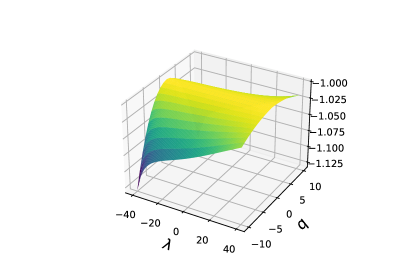
Figure 2: Value function $v$ as in (33) for $p=x=0$.

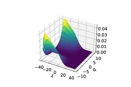
Figure 3: Certainty Equivalent for a trader who receives a signal with probability $\hat{p}=0.2$ compared to a trader without signal for spread $0.01$.

The value function is symmetric about $q=0$ due to the symmetry of (7) and (18) with respect to buy and sell orders. Hence, the expected utility of terminal wealth for an acquisition or liquidation programme is the same — everything else being equal.

Moreover, the value function is increasing in the liquidity $\lambda$ because execution costs decrease as the liquidity in the market increases. When liquidity approaches the liquidity trigger $\underline{\lambda}$, the value function is the steepest because of the additional risk of entering an auction through a market shutdown.

Similarly, the value function is particularly steep for large values of $|q|$ because a large execution programme is linked to higher risk in price and liquidity changes.

Figure 3 illustrates the signal specific certainty equivalent of the value function when the probability of receiving a signal is $\hat{p}=0.2$. It corresponds to the additional amount of initial wealth that is needed when the trader does not receive a signal to achieve the same expected utility as in the case with signal, i.e., the certainty equivalent $CE$ is such that

$$v_{\hat{p}=0}(t,q,\lambda,p,x+CE)=v_{\hat{p}=0.2}(t,q,\lambda,p,x).$$ (37)

We rearrange (37) to write

$$CE=-\frac{1}{\gamma}\log\left(\frac{v_{p=0.2}(t,q,\lambda,p,x)}{v_{p=0}(t,q,\lambda,p,x)}\right).$$ (38)

The certainty equivalent is symmetric about $q$ and does not depend on $p$ or $x$. Moreover, we see that the signal is worth the most for large $|q|$, i.e., the signal is more valueable for larger values of inventory. At most, the trader can make up to four cents from the information of the signal which corresponds to four times the bid-ask spread, see Figure 3.

The certainty equivalent is decreasing in the liquidity component $\lambda$ because as liquidity decreases, the execution times become more relevant as price impact is more costly.

Moreover, the certainty equivalent slightly increases towards the liquidity trigger $\underline{\lambda}=-40$. Here, the signal warns the trader of potentially reaching the lower bound $\underline{\lambda}$ and reduces the risk of executing a final trade in an auction.

For liquidity greater than twenty, the certainty equivalent is zero, i.e., the signal does not add any value because, with and without a signal, a trader will immediately complete the execution programme.

Benchmark — The signal optimises times of execution and trading volume.

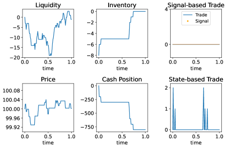
Figure 4: Optimal acquisition of eight lots. Pathwise plot when trader does not receive a signal and with spread 0.01.

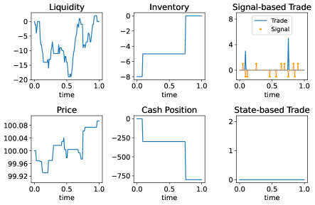
Figure 5: Optimal acquisition of eight lots. Pathwise plot when trader receives signal with probability $\hat{p}=0.2$ and with spread 0.01.

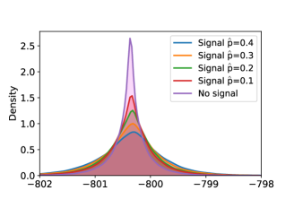
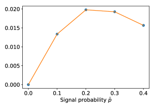
Figure 6: Optimal acquisition of eight lots. Performance of trader without signal compared to a trader who receives a signal with probability $\hat{p}\in\{0,1,0.2,0.3,0.4\}$ and with spread 0.01.
Left: Distribution of terminal wealth.  Right: Signal-Sharpe-ratio.

In the benchmark with spread 0.01, we look at the optimal acquisition problem where the trader acquires eight lots of the asset over the time horizon $[0,T]$, so the initial inventory is $q=-8$. The trader can buy and sell any multiple of lots and can execute speculative trades by trading away from the target of buying only eight lots over the trading window.

When there is no private signal, the trader sends child orders of at most two lots when liquidity is sufficiently high, see Figure 4. However, when the trader receives private signals, she times her execution times with those of the signal with information about liquidity taking orders and optimizes the trading volume of her trades, see Figure 5 (simulated with same seed as that for results in Figure 4). Here, she executes her acquisition programme by sending two child orders of sizes three and five lots upon receiving a signal about liquidity taking when the level of liquidity is high. When liquidity is low during $t\in[0.15,0.7]$, the trader does not act upon the signal and prefers to wait for liquidity to increase. Note that only the signals about liquidity taking orders are relevant in her execution programme.

More signals lead to less execution costs and riskier strategies.

Figure 6 illustrates the performance of signal-based strategies depending on the probability of receiving a signal.

Figure 6 (left) shows the distribution of terminal wealth for different probabilities of receiving a signal compared to the distribution without signal. When the probability of receiving a signal increases, the densities shift to the right, i.e., the signal increases the expected terminal wealth by optimizing the execution. On the other hand, as the probability of receiving a signal increases, also the variance of terminal wealth increases because the trader takes more risks due to the additional information through the private signal. More precisely, knowing that she will be informed about liquidity shocks through the signal, the trader waits longer for liquidity to recover from shocks before trading to minimize price impact costs. However, this is linked to more risk because unsignaled external orders can still arrive which increases the variance of the trader’s terminal wealth.

To quantify the value of the private signal $Z$, we introduce the Signal-Sharpe-ratio (SSR)

$$SSR(Z):=\frac{\bar{X}(Z)-\bar{X}(0)}{\sigma(Z)},$$ (39)

where

$$\bar{X}(Z):=\frac{1}{n_{sim}}\sum_{j=1}^{n_{sim}}\tilde{X}^{j}_{T}(Z),\text{ }\bar{X}(0):=\frac{1}{n_{sim}}\sum_{j=1}^{n_{sim}}\tilde{X}^{j}_{T}(0)\text{ and }\sigma(Z):=\sqrt{\frac{1}{n_{sim}}\sum_{j=1}^{n_{sim}}(\tilde{X}^{j}_{T}(Z)-\bar{X}(Z))^{2}}.$$

Here, $\tilde{X}^{j}_{T}(Z)$ resp. $\tilde{X}^{j}_{T}(Z0)$ denote the terminal wealth for scenario $j\in\{1,...,n_{sim}\}$ with signal $Z$ and without signal.

Precisely, the SSR is the excess return $\bar{X}(Z)-\bar{X}(0)$ for a trader with signal $Z$ compared to a trader without signal weighted by the risk $\sigma(Z)$ of a trader with signal $Z$.

Figure 6 (right) shows the SSR as a function of the probability $p$ of receiving a signal. The SSR increases up to $\hat{p}=0.2$ and slowly decreases thereafter because the increase in variance dominates the increase in expected terminal wealth which leads to a non-monotonicity in Figure 6 (left). Note that the mean-variance-optimization is not the objective of the trader who maximizes expected utility of terminal wealth, see (33).

Signal is more valuable for speculation as bid-ask spread narrows.

Next, consider a bid-ask spread of size 0.002, i.e., the bid-ask spread is one fifth of that in the benchmark. In this case, the signal incentivises speculative trades because, everything else being equal, the costs to execute roundtrip trades are lower.

The speculative roundtrip trades start after receiving a signal on liquidity provision, i.e., when the trader knows through the signal that the speculation can be unwound at better liquidity, see Figure 7. After triggering liquidity provision through her own market order, the trader waits for liquidity to arrive in the market to unwind the speculative position with better liquidity upon receiving a signal about a liquidity taking order.

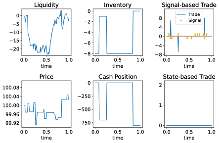
Figure 7: Optimal acquisition of eight lots. Pathwise plot when trader receives a signal with probability $\hat{p}=0.2$ and with spread $0.002$.

Next, we study the number of paths with speculative trades among $n_{sim}=100,000$ simulated paths with bid-ask spread 0.01 and 0.002 in the acquisition ($q=-8$) and pure speculation ($q=0$) scenario where the paths for wide and narrow spreads are simulated with the same seed.

When the spread is wide, i.e., when the spread is $0.01$, there is no speculation because roundtrip trades are too costly. On the other hand, when the spread is narrow, i.e., when the spread is $0.002$, there is speculation in about $21\%$ of paths in the acquisition problem ($q=-8$) and in about $11\%$ of paths in the pure speculation scenario ($q=0$). There are more speculative paths in the execution example because the trader’s execution of trades triggers liquidity provision and speculative trades become profitable. Especially, when the trader trades towards a position close to zero very early in the trading window, i.e., completes the acquisition problem early on, the remaining time horizon is long enough so that a speculative roundtrip starting close to zero is profitable; and vice versa if the trader completes the acquisition at a later point in the trading window.

Finally, without signal, there is no speculation for both the wide and the narrow bid-ask spread.

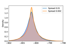
Figure 8: Optimal acquisition of eight lots. Distribution of terminal wealth when trader receives a signal with probability $\hat{p}=0.2$ with a spread of $0.01$ and $0.002$.

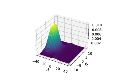
Figure 9: Certainty equivalent for a small spread of $0.002$ minus the certainty equivalent for a spread of $0.01$.

Figure 9 shows the distribution of terminal wealth in the optimal acquisition problem of $q=-8$ when the trader receives a private signal with probability $p=0.2$, and the bid-ask spread is 0.01 and 0.002. With a narrow spread, the terminal wealth is, on average, higher because the trader pays less spread and profits from speculative trades. The terminal wealth increases the most in the interval $[-801,-800.5]$, see Figure 9, because low level of liquidity, which cause smaller values of terminal wealth for a spread of $0.01$ due to price impact costs, can lead to profitable roundtrips when the spread is at $0.002$. Similarly, the variance of terminal wealth decreases because in general, the trader executes more orders to bring her inventory to zero and only deviates from this target in about $21\%$ of cases.

Similarly, Figure 9 illustrates the certainty equivalent as in (38) for spread 0.002 minus the certainty equivalent as in (38) for spread 0.01. The certainty equivalent improves when liquidity is low and when the trader’s inventory is close to zero which is when speculative trades are executed.

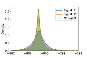
Figure 10: Optimal acquisition of eight lots. Distribution of terminal wealth for trader who receives a signal on liquidity taking (LT) with probability $\hat{p}=0.2$ vs a trader who receives a signal on liquidity provision (LP) with probability $\hat{p}=0.2$; spread is 0.01.

Signal on liquidity taking orders vs signal on liquidity providing orders.

Finally, we compare the performance of the strategy of a trader who receives a signal about the arrival of liquidity taking orders against the strategy of a trader who receives a signal about the arrival of liquidity provision.

The trader with a signal on liquidity taking uses the signal to optimize the execution times and trading volumes which increases the terminal wealth and its variance, see Figure 10. Whereas, similarly to Figure 5, the trader does not use the signal about liquidity provision for her execution so her terminal wealth coincides with that of the trader who receives no signal, see Figure 10.

4 Appendix

In this Appendix, we present the definition of the state process in the market with circuit breaker, the derivation of the HJB, the numerical scheme, and other more detailed model specifications. Moreover, we also give the proofs that were skipped in the main part of the paper.

4.1 State process in the market with circuit breaker

First, recall the specification of the state process $S^{C}_{t}=(\lambda^{C},Q^{C}_{t},P^{C}_{t},X^{C}_{t})$ and the set of admissible strategies $\mathcal{C}$ as defined in Section 2.2 for the market without circuit breaker. When introducing a circuit breaker, we denote the new state process by $\tilde{S}^{C}_{t}=(\tilde{\lambda}^{C},\tilde{Q}^{C}_{t},\tilde{P}^{C}_{t},\tilde{X}^{C}_{t})$ and the new set of admissible strategies by $\tilde{\mathcal{C}}$ which are defined as follows:

First, the set of admissible strategies in the market with circuit breaker is

$$\tilde{\mathcal{C}}=\Big{\{} C_{t}\in\mathcal{C}:\;\Delta^{l}_{t}C\text{ is }D(\lambda^{C}_{t-})\text{-valued},\;\Delta^{r}_{t}C\text{ is }D(\lambda^{C}_{t})\text{-valued},\text{ and }C_{t}=C_{\tau^{C}+}\text{ for }t>\tau^{C}\Big{\}},$$ (40)

where $\mathcal{C}$ is as in (13) and where the stopping time $\tau^{C}$ describes the point in time when the circuit breaker is triggered, i.e.,

$$\tau^{C}:=\inf\Big{\{}t\geq 0:\min\{\lambda^{C}_{t-}-|\Delta^{l}_{t}C|,\lambda^{C}_{t}\}<\underline{\lambda}\Big{\}},$$ (41)

with $\inf\emptyset=+\infty$. Moreover, we denote the set of admissible actions for liquidity level $\lambda$ as

$$D(\lambda):=D\cup\{\lambda-\underline{\lambda},\underline{\lambda}-\lambda\}.$$ (42)

Here, the enlargement by $\{\lambda-\underline{\lambda},\underline{\lambda}-\lambda\}$ ensures that the trader always has the possibility to deplete the available liquidity in the market without activating the circuit breaker, even if this deviates from trading in multiples of a lot size $\delta>0$.

Note that in (40) the condition $C_{t}=C_{\tau^{C}+}\text{ for }t>\tau^{C}$ ensures that the circuit breaker cannot be triggered by the trader’s continuous trades $dC^{c}$, but only by a signal-based trade $\Delta^{l}_{\tau^{C}}C$, a state-based trade $\Delta^{r}_{\tau^{C}}C$ or by an external market order or a cancellation of limit orders.

Next, we define the operator $\Upsilon$ for market liquidity $\lambda$ and trade size $\Delta\in\mathbb{R}$ as

$$\Upsilon(\Delta,\lambda):=\begin{cases}\hfill\Delta,&\text{if }\lambda-|\Delta|\geq\underline{\lambda},\\ \operatorname*{sgn}(\Delta)(\lambda-\underline{\lambda})^{+},&\text{if }\lambda-|\Delta|<\underline{\lambda}.\end{cases}$$ (43)

It returns $\Delta$ if the liquidity is sufficient to fill the order $\Delta$, but it returns $\lambda-\underline{\lambda}$ if $\Delta$ depletes liquidity below the level $\underline{\lambda}$ and zero if the circuit breaker has already been triggered. Here, we denote $(x)^{+}:=\max(x,0)$ for $x\in\operatorname*{\mathbb{R}}$.

Thus, we denote $\tilde{S}^{C}_{t}:=(\tilde{\lambda}^{C}_{t},\tilde{Q}^{C}_{t},\tilde{P}^{C}_{t},\tilde{X}^{C}_{t})$ the state process in the market with with circuit breaker which starts in $\tilde{S}^{C}_{0-}:=(\tilde{\lambda}^{C}_{0-},\tilde{Q}^{C}_{0-},\tilde{P}^{C}_{0-},\tilde{X}^{C}_{0-})$ and which updates according to

$$\tilde{S}^{C}_{t}:=\tilde{\mathfrak{s}}(\tilde{\lambda}^{C}_{t-},\tilde{Q}^{C}_{t-},\tilde{P}^{C}_{t-},\tilde{X}^{C}_{t-}),\quad\tilde{S}^{C}_{t+}:=\tilde{\mathfrak{s}}(\tilde{\lambda}^{C}_{t},\tilde{Q}^{C}_{t},\tilde{P}^{C}_{t},\tilde{X}^{C}_{t}),\qquad\text{ for }0\leq t\leq\tau^{C}$$ (44)

$$\text{ and }\tilde{S}^{C}_{t}=\tilde{S}^{C}_{\tau^{C}+},\qquad\text{ for }t>\tau^{C},$$ (45)

where, similarly to $\mathfrak{s}$ as in Section 2.2, the state update function $\tilde{\mathfrak{s}}$ is defined as

$$\tilde{\mathfrak{s}}(\Delta,\eta,\rho;\textbf{s}_{-}):=(\boldsymbol{\lambda},\textbf{q},\textbf{p},\textbf{x}),$$ (46)

with $$\boldsymbol{\lambda}=\begin{cases}\boldsymbol{\lambda}_{-}-|\Delta|+\mathbbm{1}_{\{\boldsymbol{\lambda}_{-}-|\Delta|\geq\underline{\lambda}\}}(-|\eta|+\rho),&\text{ if }\boldsymbol{\lambda}_{-}\geq\underline{\lambda},\\ \hfill\boldsymbol{\lambda}_{-},&\text{ if }\boldsymbol{\lambda}_{-}<\underline{\lambda},\\ \end{cases}$$ (47)

$$\textbf{q}=\textbf{q}_{-}+\Upsilon(\Delta,\boldsymbol{\lambda}_{-})$$ (48)

$$\textbf{p}=\textbf{p}_{-}-I\left(\Upsilon(\Delta,\boldsymbol{\lambda}_{-}),\boldsymbol{\lambda}_{-}\right)+\mathbbm{1}_{\{\boldsymbol{\lambda}_{-}-|\Delta|\geq\underline{\lambda}\}}I\left(\Upsilon(\eta,\boldsymbol{\lambda}_{-}-|\Delta|),\boldsymbol{\lambda}_{-}-|\Delta|\right)$$ (49)

$$\textbf{x}=\textbf{x}_{-}-\textbf{p}_{-}\Upsilon(\Delta,\boldsymbol{\lambda}_{-})-\zeta|\Upsilon(\Delta,\boldsymbol{\lambda}_{-})|-\Xi(\Upsilon(\Delta,\boldsymbol{\lambda}_{-}),\boldsymbol{\lambda}_{-}).$$ (50)

Here, $\tilde{\mathfrak{s}}(\Delta,\eta,\rho;\textbf{s}_{-})$ coincides with $\mathfrak{s}(\Delta,\eta,\rho;\textbf{s}_{-})$ when $\boldsymbol{\lambda}_{-},\boldsymbol{\lambda}\geq\underline{\lambda}$. Else, the order that pushes $\boldsymbol{\lambda}$ below $\underline{\lambda}$ is executed only partially via the function $\Upsilon$ as in (43) and trading is halted for $\boldsymbol{\lambda}$ below $\underline{\lambda}$.
Hence, as long as the circuit breaker has not been triggered yet, the state process in the market with and without circuit breaker coincide so that $\tilde{S}^{C}_{t}=S^{C}_{t}$ for $0\leq t<\tau^{C}$.

Note that for simplicity of notation, we will in the following write $\tilde{S}^{C}_{t}=(\lambda^{C}_{t},Q^{C}_{t},P^{C}_{t},X^{C}_{t})$ for the components of the state process in the market with circuit breaker.

Finally, we define the external market order flow $\tilde{M}^{C}_{t}$ in the market with circuit breaker as

$$\tilde{M}^{C}_{t} =\int_{[0,t]\times E\times\operatorname*{\mathbb{R}}_{+}}\Upsilon(\eta(e),\lambda^{C}_{s-}-|\Gamma_{s}(z(e,y))|)\mathbbm{1}_{\{y\leq f(\lambda^{C}_{s-})\}}N(ds,de,dy).$$ (51)

Similarly, the limit orders in the market with circuit breaker are

$$\tilde{L}^{C,+}_{t} =\int_{[0,t]\times E\times\operatorname*{\mathbb{R}}_{+}}\rho^{+}(e)\mathbbm{1}_{\{\lambda^{C}_{s-}-|\Gamma_{s}(z(e,y))|\geq\underline{\lambda}\}\cap\{y\leq g(\lambda^{C}_{s-})\}}N(ds,de,dy),$$ (52)

and the cancellations of limit orders in the market with circuit breaker are

$$d\tilde{L}^{C,-}_{t} =\int_{[0,t]\times E\times\operatorname*{\mathbb{R}}_{+}}\Upsilon(\rho^{-}(e),\lambda^{C}_{s-}-|\Gamma_{s}(z(e,y))|)\mathbbm{1}_{\{y\leq g(\lambda^{C}_{s-})\}}N(ds,de,dy).$$ (53)

Here, the function $\Upsilon$ in (51) and (53) as well as the indicator in (52) ensure that trading is halted after circuit breaker activation and that the order flow remains constant after $\tau^{C}$.

4.2 The Hamilton–Jacobi–Bellman equation

In the following, we derive the HJB equation that is satisfied by the value function $v$ as in (33). Particularly, we investigate for which conditions the value process $V^{C}_{t}:=v(T-t,\tilde{S}^{C}_{t+})$, $t\in[0,T]$ with arbitrary, but fixed time horizon $T$, satisfies super-martingale dynamics for every admissible $C\in\tilde{\mathcal{C}}$ and martingale dynamics for some optimal strategy $C^{*}\in\tilde{\mathcal{C}}$.

Recall the decomposition of admissible strategies from Lemma 2.3 and suppose that the value function $v(T,\lambda,q,p,x)$ is sufficiently smooth to apply Itô’s formula so that we write at least formally for $0\leq t\leq\tau^{C}\wedge T$

$$dV^{C}_{t}=-\frac{\partial v}{\partial T}(T-t,S^{C}_{t-})dt+\left(\frac{\partial v}{\partial p}(T-t,S^{C}_{t-})\iota(\lambda)-\frac{\partial v}{\partial x}(T-t,S^{C}_{t-})P^{C}_{t-}+\frac{\partial v}{\partial q}(T-t,S^{C}_{t-})\right)d\tilde{C}^{c}_{t}$$ (54)

$$+\left(\frac{\partial v}{\partial x}(T-t,S^{C}_{t-})\zeta-\frac{\partial v}{\partial\lambda}(T-t,S^{C}_{t-})\right)|d\tilde{C}^{c}_{t}|$$

$$+\int\limits_{E\times\operatorname*{\mathbb{R}}_{+}}\Big{[}v\!\left(T\!-\!t,\tilde{\mathfrak{s}}\left(\Gamma_{t}(z(e,y)),\eta(e)\mathbbm{1}_{\{y\leq f(\lambda^{C}_{t-})\}},\rho(e)\mathbbm{1}_{\{y\leq g(\lambda^{C}_{t-})\}};S^{C}_{t-}\right)\right)\!-\!v\!\left(T\!-\!t,S^{C}_{t-}\right)\Big{]}\bar{N}(dt,de,dy)$$

$$+\int\limits_{E\times\operatorname*{\mathbb{R}}_{+}}\Big{[}v\!\left(T\!-\!t,\tilde{\mathfrak{s}}\left(\Gamma_{t}(z(e,y)),\eta(e)\mathbbm{1}_{\{y\leq f(\lambda^{C}_{t-})\}},\rho(e)\mathbbm{1}_{\{y\leq g(\lambda^{C}_{t-})\}};S^{C}_{t-}\right)\!\right)\!-\!v\!\left(T\!-\!t,S^{C}_{t-}\right)\!\Big{]}(\nu(de)\otimes dy)dt$$

$$+\left[v\left(T-t,\tilde{\mathfrak{s}}(\Delta^{r}_{t}\tilde{C},0,0;S^{C}_{t})\right)-v\left(T-t,S^{C}_{t}\right)\right],$$

where $\bar{N}(dt,de,dy)=N(dt,de,dy)-dt\otimes\nu(de)\otimes dy$ is the compensated Poisson measure and $\partial v/\partial T$ denotes the derivative of $v$ with respect to the first component.

For $V^{C}$ to be a supermartingale for any admissible $C$, the impulse condition

$$\sup\limits_{\Delta\in D(\lambda)}\Big{\{}v(T,\tilde{\mathfrak{s}}(\Delta,0,0;s))-v(T,s)\Big{\}}\leq 0,\quad(T,s)\in[0,\infty)\times[\underline{\lambda},\infty)\times\mathbb{R}^{3},$$ (55)

must be satisfied. We decompose the $\nu(de)\otimes dy)$-integral in (54) into

$$\int\limits_{\hskip 30.0pt(E\times\operatorname*{\mathbb{R}}_{+})\cap\{z(e,y)=0\}}\left[v\!\left(T-t,\tilde{\mathfrak{s}}\left(0,\eta(e)\mathbbm{1}_{\{y\leq f(\lambda^{C}_{t-})\}},\rho(e)\mathbbm{1}_{\{y\leq g(\lambda^{C}_{t-})\}};S^{C}_{t-}\right)\right)\!-\!v\!\left(T-t,S^{C}_{t-}\right)\right]\nu(de)\otimes dy$$ (56)

$$+\int\limits_{\hskip 30.0pt(E\times\operatorname*{\mathbb{R}}_{+})\cap\{z(e,y)\neq 0\}}\Big{[}v\!\left(T\!-\!t,\tilde{\mathfrak{s}}\left(\Gamma_{t}(z(e,y)),\eta(e)\mathbbm{1}_{\{y\leq f(\lambda^{C}_{t-})\}},\rho(e)\mathbbm{1}_{\{y\leq g(\lambda^{C}_{t-})\}};S^{C}_{t-}\right)\right)\!-\!v\!\left(T\!-\!t,S^{C}_{t-}\right)\Big{]}\nu(de)\otimes dy,$$ (57)

where by Lemma 2.3 $\Gamma_{t}(z(e,y))=0$ in (56) where we have $z(e,y)=0$. For (57), we use the desintegration

$$\nu(de)\otimes dy=\int_{z(E\times\operatorname*{\mathbb{R}}_{+})\setminus\{0\}}K(\bar{z};de\otimes dy)\mu(d\bar{z}),$$

with $\mu=(\nu\otimes Leb)\circ(z)^{-1}$ to estimate the expression in (57) as follows:

$$\int\limits_{\hskip 44.0pt(E\times\operatorname*{\mathbb{R}}_{+})\cap\{z(e,y)\neq 0\}}\left[v\!\left(T\!-\!t,\tilde{\mathfrak{s}}\left(\Gamma_{t}(z(e,y)),\eta(e)\mathbbm{1}_{\{y\leq f(\lambda^{C}_{t-})\}},\rho(e)\mathbbm{1}_{\{y\leq g(\lambda^{C}_{t-})\}};S^{C}_{t-}\right)\right)\!-\!v\!\left(T\!-\!t,S^{C}_{t-}\right)\right]\nu(de)\otimes dy$$

$$=\int\limits_{z(E\times\operatorname*{\mathbb{R}}_{+})\setminus\{0\}}\int\limits_{\hskip 30.0pt(E\times\operatorname*{\mathbb{R}}_{+})\cap\{z(e,y)=\bar{z}\}}\Big{[}v\left(T-t,\tilde{\mathfrak{s}}\left(\Gamma_{t}(\bar{z}),\eta(e)\mathbbm{1}_{\{y\leq f(\lambda^{C}_{t-})\}},\rho(e)\mathbbm{1}_{\{y\leq g(\lambda^{C}_{t-})\}};S^{C}_{t-}\right)\right)$$

$$\hskip 156.49014pt-v\left(T-t,S^{C}_{t-}\right)\Big{]}K(\bar{z};de\otimes dy)\mu(d\bar{z})$$

$$\leq\int\limits_{z(E\times\operatorname*{\mathbb{R}}_{+})\setminus\{0\}}\sup_{\gamma\in D(\lambda)}\int\limits_{(E\times\operatorname*{\mathbb{R}}_{+})\cap\{z(e,y)=\bar{z}\}}\Big{[}v\left(T-t,\tilde{\mathfrak{s}}\left(\gamma,\eta(e)\mathbbm{1}_{\{y\leq f(\lambda^{C}_{t-})\}},\rho(e)\mathbbm{1}_{\{y\leq g(\lambda^{C}_{t-})\}};S^{C}_{t-}\right)\right)$$

$$\hskip 199.16928pt-v\left(T-t,S^{C}_{t-}\right)\Big{]}K(\bar{z};de\otimes dy)\mu(d\bar{z}).$$

Finally, we collect all the $dt$-terms from the dynamics of $dV^{C}_{t}$ and have the tight upper bound

$$-\frac{\partial v}{\partial T}(T-t,S^{C}_{t-})$$

$$+\!\!\!\!\int\limits_{(E\times\operatorname*{\mathbb{R}}_{+})\cap\{z(e,y)=0\}}\left[v\left(T-t,\tilde{\mathfrak{s}}\left(0,\eta(e)\mathbbm{1}_{\{y\leq f(\lambda^{C}_{t-})\}},\rho(e)\mathbbm{1}_{\{y\leq g(\lambda^{C}_{t-})\}};S^{C}_{t-}\right)\right)-v\left(T-t,S^{C}_{t-}\right)\right](\nu(de)\otimes dy)$$

$$+\!\!\!\!\int\limits_{z(E\times\operatorname*{\mathbb{R}}_{+})\setminus\{0\}}\sup_{\gamma\in D(\lambda)}\int\limits_{(E\times\operatorname*{\mathbb{R}}_{+})\cap\{z(e,y)=\bar{z}\}}\Big{[}v\left(T-t,\tilde{\mathfrak{s}}\left(\gamma,\eta(e)\mathbbm{1}_{\{y\leq f(\lambda^{C}_{t-})\}},\rho(e)\mathbbm{1}_{\{y\leq g(\lambda^{C}_{t-})\}};S^{C}_{t-}\right)\right)$$ (58)

$$\hskip 170.71652pt-v\left(T-t,S^{C}_{t-}\right)\Big{]}K(\bar{z};de\otimes dy)\mu(d\bar{z}).$$

To satisfy the martingale optimality principle, the terms in (58) must be smaller than or equal to zero for any admissible strategy $C\in\tilde{\mathcal{C}}$ and zero for some (optimal) strategy $C^{*}$. With (55), we thus obtain the following HJBQVI,

$$\max\bigg{\{}-\frac{\partial v}{\partial T}(T,s)+\int\limits_{(E\times\operatorname*{\mathbb{R}}_{+})\cap\{z(e,y)=0\}}\left[v\left(T,\tilde{\mathfrak{s}}\left(0,\eta(e)\mathbbm{1}_{\{y\leq f(\lambda)\}},\rho(e)\mathbbm{1}_{\{y\leq g(\lambda)\}};s\right)\right)-v\left(T,s\right)\right]\nu(de)\otimes dy$$

$$\quad+\int\limits_{z(E\times\operatorname*{\mathbb{R}}_{+})\setminus\{0\}}\sup_{\gamma\in D(\lambda)}\int\limits_{\hskip 30.0pt(E\times\operatorname*{\mathbb{R}}_{+})\cap\{z(e,y)=\bar{z}\}}\left[v\left(T,\tilde{\mathfrak{s}}\left(\gamma,\eta(e)\mathbbm{1}_{\{y\leq f(\lambda)\}},\rho(e)\mathbbm{1}_{\{y\leq g(\lambda)\}};s\right)\right)\!-\!v\left(T,s\right)\right]K(\bar{z};de\otimes dy)\mu(d\bar{z});$$

$$\quad\sup\limits_{\Delta\in D(\lambda)}\Big{\{}v(T,\tilde{\mathfrak{s}}(\Delta,0,0;s))-v(T,s)\Big{\}}\bigg{\}}=0,$$ (59)

for $(T,s)=(T,\lambda,q,p,x)\in[0,\infty)\times[\underline{\lambda},\infty)\times\mathbb{R}\times\operatorname*{\mathbb{R}}\times\operatorname*{\mathbb{R}}$. Due to the circuit breaker being activated when liquidity falls below $\underline{\lambda}$, the value function evaluated in $\lambda<\underline{\lambda}$ is

$$v(T,\lambda,q,p,x)=U_{\alpha}\left(x+pq-\zeta|q|-\Xi(q,\underline{\lambda})\right)\exp\left(\frac{1}{2}\alpha^{2}\sigma^{2}|q|^{2}\right),$$

$\text{for }(T,q,p,x)\in[0,\infty)\times\mathbb{R}\times\operatorname*{\mathbb{R}}\times\operatorname*{\mathbb{R}}$, and the initial condition for $s=(\lambda,q,p,x)\in\mathbb{S}$ with zero time to go $T=0$ is

$$v(0,s)=\begin{cases}U_{\alpha}\left(x+pq-\zeta|q|-\Xi(q,\lambda)\right)\exp\left(\frac{1}{2}\alpha^{2}\sigma^{2}((|q|-(\lambda-\underline{\lambda}))^{+})^{2}\right),&\text{ if }\lambda\geq\underline{\lambda},\\ U_{\alpha}\left(x+pq-\zeta|q|-\Xi(q,\underline{\lambda})\right)\exp\left(\frac{1}{2}\alpha^{2}\sigma^{2}|q|^{2}\right),&\text{ if }\lambda<\underline{\lambda}.\end{cases}$$ (60)

To reduce the dimensions of the HJB equation, we use the Ansatz

$$v(T,s)=\begin{cases}w(T,\lambda,q)|U_{\alpha}(x+pq)|,&\alpha>0,\\ \hfill w(T,\lambda,q)+x+pq,&\alpha=0,\end{cases}\qquad\forall(T,s)=(T,\lambda,q,p,x)\in[0,\infty)\times\mathbb{S}.$$ (61)

For simplicity, we introduce the notations

$$\gamma^{\lambda} :=\Upsilon(\gamma,\lambda),$$ (62)

$$\eta^{\lambda,\gamma}(e,y) :=\Upsilon(\eta(e),\lambda-|\gamma^{\lambda}|)\mathbbm{1}_{\{y\leq f(\lambda)\}},$$ (63)

$$\rho^{\lambda,\gamma}(e,y) :=\Big{(}\rho^{+}(e)\mathbbm{1}_{\{\lambda-|\gamma^{\lambda}|\geq\underline{\lambda}\}}+\Upsilon(\rho^{-}(e),\lambda-|\gamma^{\lambda}|)\Big{)}\mathbbm{1}_{\{y\leq g(\lambda)\}},$$ (64)

$$\lambda^{\lambda,\gamma}(e,y) :=\hfill\lambda-|\gamma|-|\eta(e)|\mathbbm{1}_{\{y\leq f(\lambda)\}}+\rho(e)\mathbbm{1}_{\{y\leq g(\lambda)\}},$$ (65)

$$\Delta^{\lambda} :=\Upsilon(\Delta,\lambda).$$ (66)

This allows us to write the reduced HJB for $w(T,\lambda,q)$ with $(T,\lambda,q)\in[0,\infty)\times[\underline{\lambda},\infty)\times\operatorname*{\mathbb{R}}$ when $\alpha>0$ as

$$\max \bigg{\{}-\frac{\partial w}{\partial T}(T,\lambda,q)+\int\limits_{(E\times\operatorname*{\mathbb{R}}_{+})\cap\{z(e,y)=0\}}\bigg{[}w\Big{(}T,\lambda^{\lambda,0}(e,y),q\Big{)}\Big{|}U_{\alpha}\Big{(}I(\eta^{\lambda,0}(e,y),\lambda)q\Big{)}\Big{|}-w(T,\lambda,q)\bigg{]}\nu(de)\otimes dy$$ (67)

$$+\int\limits_{z(E\times\operatorname*{\mathbb{R}}_{+})\setminus\{0\}}\sup_{\gamma\in D(\lambda)}\bigg{\{}\int\limits_{\hskip 50.0pt(E\times\operatorname*{\mathbb{R}}_{+})\cap\{z(e,y)=\bar{z}\}}\bigg{[}w\Big{(}T,\lambda^{\lambda,\gamma}(e,y),q+\gamma^{\lambda}\Big{)}\cdot$$

$$\hskip 85.35826pt\Big{|}U_{\alpha}\Big{(}\!\!-\zeta|\gamma^{\lambda}|-\Xi(\gamma^{\lambda},\lambda)+\Big{(}I\left(\gamma^{\lambda},\lambda\right)+I\big{(}\eta^{\lambda,\gamma}(e,y),\lambda-|\gamma^{\lambda}|\big{)}\Big{)}(q+\gamma^{\lambda})\Big{)}\Big{|}$$

$$\hskip 113.81102pt-w(T,\lambda,q)\bigg{]}K(\bar{z};de\otimes dy)\bigg{\}}\mu(d\bar{z});$$

$$\sup\limits_{\Delta\in D(\lambda)}\Big{\{}w(T,\lambda,q,\Delta)-w(T,\lambda,q)\Big{\}}\bigg{\}}=0.$$

For $\lambda<\underline{\lambda}$, the function $w(T,\lambda,q)$ takes the value

$$w(T,\lambda,q)=U_{\alpha}\left(-\zeta|q|-\Xi(q,\underline{\lambda})\right)\exp\left(\frac{1}{2}\alpha^{2}\sigma^{2}|q|^{2}\right),\quad(T,q)\in[0,\infty)\times\mathbb{R},$$ (68)

and the initial condition for $(\lambda,q)\in\operatorname*{\mathbb{R}}\times\operatorname*{\mathbb{R}}$ with zero time to go is

$$w(0,\lambda,q)=\begin{cases}U_{\alpha}\left(-\zeta|q|-\Xi(q,\lambda)\right)\exp\left(\frac{1}{2}\alpha^{2}\sigma^{2}((|q|-(\lambda-\underline{\lambda}))^{+})^{2}\right),&\text{ if }\lambda\geq\underline{\lambda},\\ U_{\alpha}\left(-\zeta|q|-\Xi(q,\underline{\lambda})\right)\exp\left(\frac{1}{2}\alpha^{2}\sigma^{2}|q|^{2}\right),&\text{ if }\lambda<\underline{\lambda}.\end{cases}$$ (69)

Similarly, one obtains the reduced HJB for $w$ when $\alpha=0$.
The suggested optimal strategy can as usual be constructed in feedback form by determining the maximizer in the suprema of the HJB (67).

4.3 The Numerical Scheme

In the following, we present a numerical scheme to approximate the solution of the dimension reduced HJB equation in (67) for $\alpha>0$; a similar scheme can be derived for $\alpha=0$.
First, we introduce a discretized, bounded subset of the space $[0,T]\times\mathbb{R}\times[\underline{\lambda},\infty)$:
For the time dimension $T^{\prime}\in[0,T]$, we take $\mathbb{T}_{\delta T}$ as the grid on $[0,T]$ with step size $\delta T>0$, where $T=N\delta T$ for some $N_{1}\in\mathbb{N}$.
For the liquidity component $\lambda\in[\underline{\lambda},\infty)$, we denote $\mathbb{R}_{\delta\lambda}^{\overline{\lambda}}$ the bounded grid on $[\underline{\lambda}-\delta\lambda,\overline{\lambda}]$ with stepsize $\delta\lambda>0$ where $\overline{\lambda}=\underline{\lambda}+N\delta\lambda$ for some $N_{2}\in\mathbb{N}$. To remain within a bounded domain, we assume $\lambda$ equals $\underline{\lambda}-\delta\lambda$ after the circuit breaker is triggered and define the numerical scheme below accordingly.
For inventory $q\in\mathbb{R}$, we introduce the bounded grid $\mathbb{R}_{\delta q}^{\underline{Q},\overline{Q}}$ on $[\underline{Q},\overline{Q}]$ with step size $\delta q>0$ where $\underline{Q}=N_{3}\delta q$ and $\overline{Q}=N_{4}\delta_{q}$ for some constants $N_{3},N_{4}\in\mathbb{Z}$, $N_{3}<N_{4}$.
For the inventory $q$ to remain within the grid $\mathbb{R}_{\delta q}^{\underline{Q},\overline{Q}}$ and for $\lambda$ to remain above $\underline{\lambda}-\delta\lambda$, we define the set of actions

$$D^{\underline{Q},\overline{Q}}(q,\lambda):=\Big{\{}n\cdot\delta q\text{ with }n\in\mathbb{Z}:q+n\,\delta q\in\mathbb{R}_{\delta q}^{\underline{Q},\overline{Q}}\text{ and }\lambda-|n\delta|\geq\underline{\lambda}-\delta\lambda\Big{\}},\qquad q\in\mathbb{R}_{\delta q}^{\underline{Q},\overline{Q}},\lambda\in\mathbb{R}_{\delta\lambda}^{\overline{\lambda}}.$$

For any function $h^{T^{\prime}}:\mathbb{R}_{\delta\lambda}^{\overline{\lambda}}\times\mathbb{R}_{\delta q}^{\underline{Q},\overline{Q}}\rightarrow\mathbb{R}$ with $T^{\prime}\in\mathbb{T}_{\delta T}$, we introduce the operator

$$\mathcal{L}^{\delta T,\delta\lambda}(q,\lambda,h^{T^{\prime}}):=h^{T^{\prime}}(\lambda,q)+\delta t\bigg{(}\Delta_{z=0}h^{T^{\prime}}(\lambda,q)+\int\limits_{z(E\times\mathbb{R}_{+})\setminus\{0\}}\sup\limits_{\gamma\in D^{\underline{Q},\overline{Q}}(q,\lambda)}\Delta_{\text{z=}\bar{z}}h^{T^{\prime}}(\lambda,q,\gamma,\psi)\;\;\mu(d\bar{z})\bigg{)},$$

where we use the notations

$$\Delta_{\text{z=0}}h^{T^{\prime}}(\lambda,q):=\int\limits_{(E\times\mathbb{R}_{+})\cap\{z(e,y)=0\}}\Big{[}\bar{h}^{T^{\prime}}\big{(}\lambda^{\lambda,0}(e,y)\vee(\underline{\lambda}-\delta\lambda),q\big{)}\big{|}U_{\alpha}\big{(}I(\eta^{\lambda,0}(e,y),\lambda)q\big{)}\big{|}-h^{T^{\prime}}(\lambda,q)\Big{]}\nu(de)\otimes dy,$$

$$\Delta_{\text{z=}\bar{z}}h^{t}(\lambda,q,\gamma):=$$

$$\int\limits_{\hskip 30.0pt(E\times\mathbb{R}_{+})\cap\{z(e,y)=\bar{z}\}}\bigg{[}\bar{h}^{T^{\prime}}\big{(}\lambda^{\lambda,\gamma}(e,y)\vee(\underline{\lambda}-\delta\lambda),q+\gamma^{\lambda}\big{)}\cdot\;$$

$$\hskip 17.07182pt\Big{|}U_{\alpha}\Big{(}-\zeta|\gamma^{\lambda}|-\Xi(\gamma^{\lambda},\lambda)-\big{(}I(\gamma^{\lambda},\lambda)+I\big{(}\eta^{\lambda,\gamma}(e,y),\lambda-|\gamma^{\lambda}|\big{)}\big{)}(q+\gamma^{\lambda})\Big{)}\Big{|}-h^{T^{\prime}}(\lambda,q)\bigg{]}K(\bar{z};de,dy),$$

and we interpolate for $\lambda\notin\mathbb{R}_{\delta\lambda}^{\overline{\lambda}}$

$$\bar{h}^{T^{\prime}}(q,\lambda):= h^{T^{\prime}}\left(q,\left\lceil\frac{\lambda}{\delta\lambda}\right\rceil\delta\lambda\right)-\left(\left\lceil\frac{\lambda}{\delta\lambda}\right\rceil\delta\lambda-\lambda\right)\left(h^{T^{\prime}}\left(q,\left\lceil\frac{\lambda}{\delta\lambda}\right\rceil\delta\lambda\right)-h^{T^{\prime}}\left(q,\left\lfloor\frac{\lambda}{\delta\lambda}\right\rfloor\delta\lambda\right)\right).$$

Here, $\lfloor\cdot\rfloor$ and $\lceil\cdot\rceil$ denotes rounding to the closest integer below and above. Similarly, we define

$$\mathcal{M}^{\delta T,\delta\lambda}(\lambda,q,h^{T^{\prime}}):=\sup\limits_{\Delta\in D^{\underline{Q},\overline{Q}}(q,\lambda)}\!\bigg{\{}\bar{h}^{T^{\prime}}\big{(}(\lambda-|\Delta|)\vee(\lambda-\delta\lambda),q+\Delta\big{)}\cdot$$

$$\hskip 142.26378pt\big{|}U\big{(}-\zeta|\Delta^{\lambda}|-\Xi(\Delta^{\lambda},\lambda)-I(\Delta^{\lambda},\lambda)(q+\Delta^{\lambda})\big{)}\big{|}\bigg{\}}.$$

Finally, we use the following numerical scheme to compute an approximate solution $w$ to (67)

$$w^{0}(q,\lambda) :=\begin{cases}U_{\alpha}\left(-\zeta|q|-\Xi(q,\lambda)\right)\exp\left(-\frac{1}{2}\alpha^{2}\sigma^{2}((|q|-(\lambda-\underline{\lambda}))^{+})^{2}\right),&\text{ if }\lambda\geq\underline{\lambda},\\ \hfill U_{\alpha}\left(-\zeta|q|-\Xi(q,\underline{\lambda})\right)\exp\left(-\frac{1}{2}\alpha^{2}\sigma^{2}|q|^{2}\right),&\text{ if }\lambda=\underline{\lambda}-\delta\lambda,\\ \end{cases}$$

$$\tilde{w}^{T^{\prime}+\delta T}(q,\lambda) :=\mathcal{L}^{\delta T,\delta\lambda}(q,\lambda,w^{t}),\qquad\lambda\geq\underline{\lambda},$$

$$w^{T^{\prime}+\delta T}(q,\lambda) :=\max(\tilde{w}^{T^{\prime}+\delta T}(q,\lambda),\mathcal{M}^{\delta t,\delta\lambda}(q,\lambda,\tilde{w}^{T^{\prime}+\delta T})),\qquad\lambda\geq\underline{\lambda},$$

$$w^{T^{\prime}+\delta t}(q,\lambda-\delta\lambda) :=U_{\alpha}\left(-\zeta|q|-\Xi(q,\underline{\lambda})\right)\exp\left(-\tfrac{1}{2}\alpha^{2}\sigma^{2}|q|^{2}\right)\quad\text{for}\;T^{\prime}\in\{0,\delta t,...,T-2\delta t,T-\delta t\}.$$

4.4 Formal Model Specification of Section 3.3

In this part, we link the model specification in Section 3.3 to the notations in Chapter 2. For simplicity, we only treat the benchmark; the specification of the remaining settings in Section 3.3 are similar.
First, the space $E$ is given by $E=\{-3,-2,-1,1,2,3\}\times\{1,2,3\}\times\{0,1\}$. The mappings $\eta$ and $\rho$ are

$$\eta(e)=e_{1}(1-e_{3})\quad\text{and}\quad\rho(e)=e_{2}e_{3}.$$

The model is driven by the homogenous Poisson point process $N(dt,de,dy)$ with compensator $dt\otimes\nu(de)\otimes dy$, where $\nu(de)=P^{1}(de_{1})\otimes P^{2}(de_{2})\otimes P^{3}(de_{3})$ with

$$P^{1}(\{-3\})=P^{1}(\{3\})=0.1,\quad P^{1}(\{-2\})=P^{1}(\{2\})=P^{1}(\{-1\})=P^{1}(\{1\})=0.2,$$ (70)

$$P^{2}(\{1\})=P^{2}(\{1\})=0.4,\quad P^{2}(\{3\})=0.2,$$ (71)

$$P^{3}(\{0\})=P^{3}(\{1\})=0.5.$$ (72)

The signal $Z_{t}\in(\{-1,1\}\times\mathbb{R}_{+})^{\mathbb{N}}$ is given as the vector $Z_{t}=(Z_{t}^{n})_{n\in\mathbb{N}}$, with $Z^{n}=(Z^{n,1}_{t},Z^{n,2}_{t})\in\{-1,1\}\times\mathbb{R}_{+}$, defined as

$$Z^{n}_{t}:=\int_{[0,T]\times E\times\operatorname*{\mathbb{R}}_{+}}z^{n}(e,y)N(ds,de,dy),$$ (73)

$$\text{where }z^{n}(e,y)=(-\mathbbm{1}_{\{e_{3}=0\}}+\mathbbm{1}_{\{e_{3}=1\}},y\mathbbm{1}_{[n-1,n]}(y)).$$ (74)

We disintegrate for $\bar{z}=(\bar{z}^{n})_{n\in\mathbb{N}}\in(\{-1,1\}\times\mathbb{R}_{+})^{\mathbb{N}}$, with $\bar{z}^{n}=(\bar{z}^{n,1},\bar{z}^{n,2})$,

$$\nu(de)\otimes dy=\int_{z(E\times\operatorname*{\mathbb{R}}_{+})}K(\bar{z};de,dy)\mu(d\bar{z}),$$ (75)

where

$$\mu(d\bar{z}) =\sum_{n\in\mathbb{N}}\mu^{n}(d\bar{z}^{n}),$$ (76)

$$\mu^{n}(d\bar{z}) =(\nu\otimes Leb_{\big{|}[n-1,n]}\,)\circ z^{-1}(\bar{z}^{n}),$$ (77)

$$K(\bar{z};de,dy) =\mathbbm{1}_{\{\bar{z}_{1}=-1\}}(P^{1}\otimes P^{2}\otimes\text{Dirac}_{\{0\}})(de)\otimes\text{Dirac}_{\sum_{n\in\mathbb{N}}\bar{z}^{n,2}}(dy)$$ (78)

$$\quad+\mathbbm{1}_{\{\bar{z}_{1}=1\}}(P^{1}\otimes P^{2}\otimes\text{Dirac}_{\{1\}})(de)\otimes\text{Dirac}_{\sum_{n\in\mathbb{N}}\bar{z}^{n,2}}(dy).$$ (79)

Here, $\bar{z}_{1}$ and $\bar{z}_{2}$ denote the first and second component of the signal.

4.5 Proofs

Lemma 2.1 - The uncontrolled model dynamics admit a unique solution

Proof of Lemma 2.1.

It suffices to rule out that the mutually-exciting dynamics lead to blow-ups.
To this end, we prove that the expectation of the total variation $V_{[0,t]}(\lambda)$ of the liquidity process $\lambda$ on $[0,t]$ is bounded for each $t\in[0,T]$.
Let $c_{1},c_{2}$ be the constants as in (4). We use that $\eta,\rho\in L^{1}(\nu)$ to bound the expected variation of $\lambda$ for every $t\in[0,T]$ from above

$$\mathbb{E}[V_{[0,t]}(\lambda)]$$

$$\leq\mathbb{E}\left[\int_{[0,t]\times E\times\mathbb{R}_{+}}\!\!\mathbbm{1}_{\{y\leq g(\lambda_{s-})\}}|\rho(e)|N(ds,de,dy)+\int_{[0,t]\times E\times\mathbb{R}_{+}}\!\!\mathbbm{1}_{\{y\leq f(\lambda_{s-})\}}|\eta(e)|N(ds,de,dy)\right]$$

$$=\int_{E}|\rho(e)|\nu(de)\mathbb{E}\left[\int_{0}^{t}g(\lambda_{s})ds\right]+\int_{E}|\eta(e)|\nu(de)\mathbb{E}\left[\int_{0}^{t}f(\lambda_{s})ds\right]$$

$$\leq\left(\int_{E}|\rho(e)|\nu(de)+\int_{E}|\eta(e)|\nu(de)\right)\left(Tc_{1}+c_{2}T|\lambda_{0}|+\mathbb{E}\left[\int_{0}^{t}V_{[0,s]}(\lambda)ds\right]\right).$$

Apply Gronwall’s inequality to obtain the uniform upper bound for all $t\in[0,T]$

$$\mathbb{E}[V_{[0,t]}(\lambda)]$$

$$\leq \left(\int_{E}|\rho(e)|\nu(de)+\int_{E}|\eta(e)|\nu(de)\right)\left(Tc_{1}+c_{2}T|\lambda_{0}|\right)\exp\left(T\int_{E}|\rho(e)|\nu(de)+T\int_{E}|\eta(e)|\nu(de)\right).$$

∎

Lemma 2.2 — Link between price volatility and liquidity of the market

Proof.

The quadratic variation of the price process has dynamics

$$d[P]_{t}= \int_{E}\mathbbm{1}_{\{y\leq f(\lambda_{t-})\}}I(\eta(e),\lambda_{t-})^{2}N(dt,de,dy),\quad[P]_{0}=0.$$ (80)

Hence, the dynamics of its predictable compensator coincide with (8). The derivative of the expression in (9) with respect to $\lambda$ is negative if condition (10) holds; this proves the monotonicity claim. ∎

Lemma 2.3 — Decomposition of $C$

Proof of Lemma 2.3.

It is easy to see that $C$ of the form (14) is $\Lambda$-measurable and has bounded expected total variation.
To prove the reverse, we have to show that for a $\Lambda$-measurable process $C$ of bounded expected variation, there exists a $\mathcal{P}(\mathcal{F})\otimes\mathcal{B}(\mathbb{R})$-measurable field $\Gamma$ which satisfies the integrability condition (16) and vanishes at zero such that (15) holds.
From a monotone class argument, see [Bank and Körber, 2022, Lemma 2.2], we know that there exists a $\mathcal{P}(\mathcal{F})\otimes\mathcal{B}(\mathbb{R})$-measurable field $\Gamma$ such that $\Delta^{l}_{t}C=\Gamma_{t}(\Delta_{t}Z)$, $t\in[0,T]$. Next, because $C$ is of bounded variation, we conclude that $\Gamma_{t}(0)=0$ for all $t\in[0,T]$. Moreover, $\Gamma$ satisfies (16) because $C$ is of bounded total variation and $\Delta Z_{s}=0$ for all but countably many times. We finish the proof by

$$\Delta^{l}_{t}C=\Gamma_{t}(\Delta_{t}Z)=\int_{E\times\mathbb{R}_{+}}\Gamma_{t}(z(e,y))N(dt,de,dy),\quad t\in[0,T].$$ (81)

∎

An upper bound for the available liquidity in the market with circuit breaker

Let us note that

$$\bar{V}(T):=\lambda_{0}-\underline{\lambda}+\int_{[0,T]\times E\times\mathbb{R}_{+}}\mathbbm{1}_{\{y\leq g(\underline{\lambda})\}}|\rho(e)|N(dt,de,dy)$$ (82)

yields an upper bound for the liquidity to arrive at the market over the time period $[0,T]$. Here, $g(\underline{\lambda})$ is an upper bound for $g(\lambda)$ because we have $\lambda\geq\underline{\lambda}$ and because the function $g$ is decreasing.

Lemma 3.1 - Finite expected $n$-th moment of the total variation of liquidity taking orders in the market with circuit breaker

Proof of Lemma 3.1.

Let $\rho\in L^{n}(\nu)$ for some $n\in\mathbb{N}$. First, use that market orders and cancellations are executed as long as liquidity remains greater than $\underline{\lambda}$ to write

$$\underline{\lambda}\leq\lambda_{T}=\lambda_{0}-V_{[0,T]}(Q^{C})-V_{[0,T]}(\tilde{M}^{C})-V_{[0,T]}(\tilde{L}^{C,-})+V_{[0,T]}(\tilde{L}^{C,+}),$$ (83)

with $\tilde{M}^{C}$, $\tilde{L}^{C,+}$, $\tilde{L}^{C,-}$ as in (51), (52) and (53). By rearranging (83), we find the uniform upper bound

$$V_{[0,T]}(Q^{C})+V_{[0,T]}(\tilde{M}^{C})+V_{[0,T]}(\tilde{L}^{C,-})$$

$$\leq\lambda_{0}-\underline{\lambda}+V_{[0,T]}(\tilde{L}^{C,+})$$

$$\leq´\lambda_{0}-\underline{\lambda}+\int_{[0,T]\times E\times\mathbb{R}_{+}}\mathbbm{1}_{\{y\leq g(\underline{\lambda})\}}|\rho(e)|N(dt,de,dy)=\overline{V}(T),$$

with $\bar{V}(T)$ as in (82). We apply the Cauchy Schwarz inequality and finish the proof:

$$\mathbb{E}\left[\left(V_{[0,T]}(Q^{C})+V_{[0,T]}(\tilde{M}^{C})+V_{[0,T]}(\tilde{L}^{C,-})\right)^{n}\right]\leq\mathbb{E}\left[\overline{V}(T)^{n}\right]$$

$$\leq(n+1)(\lambda_{0}-\underline{\lambda})^{n}+(n+1)(T\nu(E)g(\underline{\lambda}))^{n-1}\mathbb{E}\left[\int_{[0,T]\times E\times[0,g(\underline{\lambda})]}|\rho(e)|^{n}N(dt,de,dy)\right]$$

$$=(n+1)(\lambda_{0}-\underline{\lambda})^{n}+(n+1)(Tg(\underline{\lambda}))^{n}\nu(E)^{n-1}\int_{E}|\rho(e)|^{n}\nu(de).$$

∎

Preliminaries for the proofs of Proposition 3.2 and Theorem 3.3

Here, we provide an overview of estimates that are used to prove Lemma 3.1, Proposition 3.2 and Theorem 3.3. First, with $\bar{V}$ as in (82) and by Lemma 3.1, we conclude that for every admissible strategy $Q\in\mathcal{Q}$

$$V_{[0,T]}(Q^{C})\leq\overline{V}(T)\quad\text{ and }\quad\sup_{t\in[0,T]}|Q^{C}_{t}|\leq|q|+\overline{V}(T).$$ (84)

Because $\iota$ is decreasing, we have for every $\lambda\in\mathbb{R}$ and $\Delta\in\mathbb{R}$

$$|I(\Delta,\lambda)|\leq\iota(\underline{\lambda})|\Delta|,\quad|\Xi(\Delta,\lambda)|\leq\iota(\underline{\lambda})|\Delta|^{2}.$$ (85)

Thus, we conclude

$$V_{[0,T]}(P^{C})\leq\iota(\underline{\lambda})\overline{V}(T)\quad\text{ and }\quad\sup_{t\in[0,T]}|P^{C}_{t}|\leq|p|+\iota(\underline{\lambda})\overline{V}(T).$$ (86)

Next, for $\lambda_{1},\lambda_{2}>\underline{\lambda}$ and $\Delta,\Delta_{1},\Delta_{2}\in\mathbb{R}$, we suppose Lipschitz continuity of $\iota$ with Lipschitz constant $c_{\iota}$ to bound the difference of $I$ as in (7) from above

$$|I(|\Delta|,\lambda_{1})-I(|\Delta|,\lambda_{2})|\leq c_{\iota}|\Delta||\lambda_{1}-\lambda_{2}|,$$ (87)

$$|I(|\Delta_{1}|,\lambda_{1})-I(|\Delta_{2}|,\lambda_{2})|\leq c_{\iota}\min(|\Delta_{1}|,|\Delta_{2}|)|\lambda_{1}-\lambda_{2}|+\iota(\underline{\lambda})|\Delta_{1}-\Delta_{2}|.$$

Similarly, we have for $\Xi$ as in (18)

$$|\Xi(\Delta,\lambda_{1})-\Xi(\Delta,\lambda_{2})|\leq c_{\iota}|\Delta|^{2}|\lambda_{1}-\lambda_{2}|,$$ (88)

$$|\Xi(\Delta_{1},\lambda_{1})-\Xi(\Delta_{2},\lambda_{2})|\leq c_{\iota}\min(|\Delta_{1}|,|\Delta_{2}|)|\lambda_{1}-\lambda_{2}|+\iota(\underline{\lambda})\max(|\Delta_{1}|,|\Delta_{2}|)|\Delta_{1}-\Delta_{2}|.$$

Lemma 4.1.

Let $\rho\in L^{2}(\nu)$ and assume starting values $(\lambda,q,p,x)$ for $(\lambda^{C},Q^{C},P^{C},X^{C})$. There exists a uniform constant $c=c(T,\lambda,q,p,x)>-\infty$ that depends continuously on its arguments such that

$$\inf_{C\in\tilde{\mathcal{C}}}\mathbb{E}\left[U_{\alpha}(\tilde{X}^{C}_{T})\right]\geq c.$$ (89)

Proof.

Let $(\lambda,q,p,x)$ be a set of starting values for $(\lambda^{C},Q^{C},P^{C},X^{C})$. For simplicity, we denote by $c=c(T,q,\lambda,p,x)>0$ a generic constant that depends continuously on $T,q,\lambda,p,x$ and that may change from line to line.
First, with (84) and (86), we write for the cash position $X^{C}_{T}$ from trading over the time horizon $[0,T]$:

$$X^{C}_{T} \geq x-\sup_{t\in[0,T]}|P^{C}_{t}|V_{[0,T]}(Q^{C})-\zeta V_{[0,T]}(Q^{C})-\iota(\underline{\lambda})V_{[0,T]}(Q^{C})^{2}.$$ (90)

Similarly, we have for the cash from completing the execution programme at time $T$:

$$\qquad-P^{C}_{T}Q^{C}_{T}-\sigma Y\operatorname*{sgn}(Q^{C}_{T})(|Q^{C}_{T}|-(\lambda^{C}_{T}-\underline{\lambda})^{+})^{+}-\zeta|Q^{C}_{T}|-\Xi(|Q^{C}_{T}|,\lambda_{T})$$ (91)

$$\geq-(\sup_{t\in[0,T]}|P^{C}_{t}|+\sigma|Y|+\zeta)(|q|+V_{[0,T]}(Q^{C}))-\iota(\underline{\lambda})(|q|+V_{[0,T]}(Q^{C}))^{2}.$$

We aggregate (90) and (91) and apply the estimates from (84) and (86) to bound $\tilde{X}^{C}_{T}$ from below

$$\tilde{X}^{C}_{T}\geq-c(|Y|+\overline{V}(T)+|Y|\overline{V}(T)+\overline{V}(T)^{2}).$$ (92)

For $\alpha=0$, the claim follows using Lemma 3.1 for $n=2$.
For $\alpha>0$, we use the monotonocity of $U_{\alpha}$ together with (92) to estimate

$$\mathbb{E}[U_{\alpha}(\tilde{X}^{C}_{T})] \geq-\mathbb{E}\bigg{[}\exp\Big{(}\alpha c(|Y|+\overline{V}(T)+|Y|\overline{V}(T)+\overline{V}(T)^{2})\Big{)}\bigg{]}$$ (93)

$$=-\mathbb{E}\bigg{[}\mathbb{E}\Big{[}\exp\Big{(}\alpha c(|Y|+|Y|\overline{V}(T))\Big{)}\Big{|}\overline{V}(T)\Big{]}\exp\Big{(}\alpha c(\overline{V}(T)+\overline{V}(T)^{2})\Big{)}\bigg{]}$$ (94)

$$=-\mathbb{E}\bigg{[}2\Phi(\alpha c(1+\overline{V}(T)))\exp\Big{(}\frac{\alpha^{2}c^{2}}{2}(1+\overline{V}(T))^{2}\Big{)}\exp\Big{(}\alpha c(\overline{V}(T)+\overline{V}(T)^{2})\Big{)}\bigg{]},$$ (95)

where we use the moment generating function of a folded normal distribution and where $\Phi$ is the cumulative distribution function of a Gaussian distribution. Next, use that $\Phi\leq 1$ to write for some constant $c$

$$\mathbb{E}[U_{\alpha}(\tilde{X}^{C}_{T})] \geq-c\>\mathbb{E}\bigg{[}\exp\Big{(}c(1+\overline{V}(T)^{2})\Big{)}\bigg{]}$$ (96)

To estimate this expresssion, we write

$$\mathbb{E}\Big{[}\exp\Big{(}c\overline{V}(T)^{2}\Big{)}\Big{]} =\mathbb{E}\left[\exp\Big{(}c\Big{(}(\lambda-\underline{\lambda})+\int_{[0,T]\times E\times[0,g(\underline{\lambda})]}|\rho(e)|N(dt,de,dy)\Big{)}^{2}\Big{)}\right]$$ (97)

$$\leq\mathbb{E}\left[\exp\Big{(}3c\Big{(}(\lambda-\underline{\lambda})^{2}+\Big{(}\int_{[0,T]\times E\times[0,g(\underline{\lambda})]}|\rho(e)|N(dt,de,dy)\Big{)}^{2}\Big{)}\Big{)}\right].$$ (98)

Next, we apply the Cauchy Schwarz inequality and have with the Lévy-Khintchine formula

$$\mathbb{E}\left[\exp\Big{(}3c\Big{(}(\lambda-\underline{\lambda})^{2}+\Big{(}\int_{[0,T]\times E\times[0,g(\underline{\lambda})]}|\rho(e)|N(dt,de,dy)\Big{)}^{2}\Big{)}\Big{)}\right]$$ (99)

$$\leq\exp\left(3c(\lambda-\underline{\lambda})^{2}\right)\mathbb{E}\left[\exp\Big{(}3cTg(\underline{\lambda})\nu(E)\int_{[0,T]\times E\times[0,g(\underline{\lambda})]}|\rho(e)|^{2}N(dt,de,dy)\Big{)}\right]$$ (100)

$$=\exp\left(3c(\lambda-\underline{\lambda})^{2}\right)\exp\left(Tg(\underline{\lambda})\int_{E}\Big{[}\exp(3cTg(\underline{\lambda})\nu(E)|\rho(e)|^{2})-1\Big{]}\nu(de)\right)<\infty,$$ (101)

where we use (35). This finishes the proof. ∎

Proposition 3.2 - The value function is non-degenerate

We use Lemma 3.1 to prove that the value function as in (33) is non-degenerate, i.e., $v<U_{\gamma}(+\infty)$.

Proof of Proposition 3.2.

Let $(\lambda,q,p,x)$ be a set of starting values for $(\lambda^{C},Q^{C},P^{C},X^{C})$.
By the concavity of $U_{\alpha}$ and with Jensen’s inequality, the claim follows if there exists a uniform, finite constant $c=c(T,q,\lambda,p,x)$ such that

$$\sup_{C\in\tilde{\mathcal{C}}}\mathbb{E}\Big{[}|\tilde{X}^{C}_{T}|\Big{]}\leq c.$$ (102)

By the triangle inequality, it is hence sufficient to prove

$$\sup_{C\in\tilde{\mathcal{C}}}\Big{(}\mathbb{E}\left[|X^{C}_{T}|\right]+\mathbb{E}\left[|P^{C}_{T}||Q^{C}_{T}|\right]+\mathbb{E}\left[|\sigma Y||Q^{C}_{T}|\right]+\mathbb{E}\left[\zeta|Q^{C}_{T}|\right]+\mathbb{E}\left[\Xi(|Q^{C}_{T}|,\lambda_{T})\right]\Big{)}\leq c.$$ (103)

For simplicity, we denote by $c=c(T,q,\lambda,p,x)>0$ a generic constant that depends continuously on $T,q,\lambda,p,x$ and that my change from line to line. We apply Lemma 3.1 with $n=1,2$ to write

$$\mathbb{E}\left[V_{[0,T]}(Q^{C})+V_{[0,T]}(M^{C})\right]+\mathbb{E}\left[\left(V_{[0,T]}(Q^{C})+V_{[0,T]}(M^{C})\right)^{2}\right]\leq c.$$ (104)

Next, by (84) and (104), we know for every $C\in\tilde{\mathcal{C}}$

$$\mathbb{E}[|Q^{C}_{T}|]+\mathbb{E}[|Q^{C}_{T}|^{2}]\leq c.$$ (105)

Similarly, by (85), (84) and by independence of $Y$, we write

$$\mathbb{E}[\sigma|Y||Q^{C}_{T}|]+\mathbb{E}[\zeta|Q^{C}_{T}|]+\mathbb{E}[|\Xi(|Q^{C}_{T}|,\lambda_{T})|]\leq c.$$ (106)

With (86) and (104), we have

$$\mathbb{E}\left[\sup_{t\in[0,T]}|P^{C}_{t}|\right]+\mathbb{E}\left[\sup_{t\in[0,T]}|P^{C}_{t}|^{2}\right]\leq c.$$ (107)

Next, we use the Cauchy Schwarz inequality together with (105) and (107) to write

$$\mathbb{E}[|P^{C}_{T}||Q^{C}_{T}|]\leq\mathbb{E}[|P^{C}_{T}|^{2}]^{\frac{1}{2}}\mathbb{E}[|Q^{C}_{T}|^{2}]^{\frac{1}{2}}\leq c.$$

Finally, by (84), (85), (104), (107), and the Cauchy Schwarz inequality, we have

$$\mathbb{E}[|X^{C}_{T}|] \leq x+\mathbb{E}\left[\sup_{t\in[0,T]}|P^{C}_{t}|V_{[0,T]}(Q^{C})+\zeta V_{[0,T]}(Q^{C})+\iota(\underline{\lambda})V_{[0,T]}(Q^{C})^{2}\right]\leq c.$$

Aggregating the above estimates, we conclude (103). ∎

Theorem 3.3 - The value function is continuous

Proving continuity of the value function is rather involved in the present problem because neither the state nor the control space is bounded at any point in time, rendering standard arguments inapplicable. Also the circuit breaker and the Hawkes-like jump structures pose a challenge for the proof continuity.

First, consider two sets of starting values $(\lambda^{\prime},q^{\prime},p,x)$ and $(\lambda^{\prime\prime},q^{\prime\prime},p,x)$ for $(\lambda^{C}_{t},Q^{C}_{t},P^{C}_{t},X^{C}_{t})$ and let $T^{\prime},T^{\prime\prime}\geq 0$. For simplicity and without loss of generality, we treat the case where p=x=0, a generalization is straight forward using (61). Let $\varepsilon>0$ and let $C^{\prime}$ be an $\varepsilon$-optimal strategy for the values $(T^{\prime},\lambda^{\prime},q^{\prime},p,x)$, and $C^{\prime\prime}$ some strategy for $(T^{\prime\prime},\lambda^{\prime\prime},q^{\prime\prime},p,x)$.
By concavity of the utility function $U_{\alpha}$, the first Taylor approximation is an upper bound for the difference of the value functions for $\alpha>0$:

$$\Big{(}w(T^{\prime},\lambda^{\prime},q^{\prime})-w(T^{\prime\prime},\lambda^{\prime\prime},q^{\prime\prime})\Big{)}=v(T^{\prime},\lambda^{\prime},q^{\prime},p,x)-v(T^{\prime\prime},\lambda^{\prime\prime},q^{\prime\prime},p,x)$$ (108)

$$\leq\mathbb{E}\left[U_{\alpha}(\tilde{X}^{C^{\prime}}_{T^{\prime}})\right]+\varepsilon-\mathbb{E}\left[U_{\alpha}(\tilde{X}^{C^{\prime\prime}}_{T^{\prime\prime}})\right]\leq\mathbb{E}\left[\alpha\exp(-\alpha\tilde{X}^{C^{\prime\prime}}_{T^{\prime\prime}})(\tilde{X}^{C^{\prime}}_{T^{\prime}}-\tilde{X}^{C^{\prime\prime}}_{T^{\prime\prime}})\right]+\varepsilon.$$ (109)

We rearrange the terms and apply the Cauchy Schwarz inequality to write

$$w(T^{\prime},\lambda^{\prime},q^{\prime})-w(T^{\prime\prime},\lambda^{\prime\prime},q^{\prime\prime})\leq\exp(\alpha(x+pq))\alpha\mathbb{E}\left[\exp(-2\alpha\tilde{X}^{C^{\prime\prime}}_{T^{\prime\prime}})\right]^{1/2}\mathbb{E}\left[(\tilde{X}^{C^{\prime}}_{T^{\prime}}-\tilde{X}^{C^{\prime\prime}}_{T^{\prime\prime}})^{2}\right]^{1/2}+\varepsilon,$$ (110)

From Lemma 4.1, we know that there exists a finite constant $c>0$ depending continuously on $(T^{\prime\prime},\lambda^{\prime\prime},q^{\prime\prime})$ such that

$$\mathbb{E}\left[\exp(-2\alpha\tilde{X}^{C^{\prime\prime}}_{T^{\prime\prime}})\right]\leq c.$$

Consequently, we obtain the estimate

$$w(T^{\prime},\lambda^{\prime},q^{\prime})-w(T^{\prime\prime},\lambda^{\prime\prime},q^{\prime\prime})\leq c\mathbb{E}\left[(\tilde{X}^{C^{\prime}}_{T^{\prime}}-\tilde{X}^{C^{\prime\prime}}_{T^{\prime\prime}})^{2}\right]^{1/2}+\varepsilon,$$ (111)

where $c>0$ is a finite constant depending continuously on $(T^{\prime\prime},\lambda^{\prime\prime},q^{\prime\prime})$.
For $\alpha=0$, we have the estimate

$$w(T^{\prime},\lambda^{\prime},q^{\prime})-w(T^{\prime\prime},\lambda^{\prime\prime},q^{\prime\prime}) \leq\mathbb{E}\left[\tilde{X}^{C^{\prime}}_{T^{\prime}}-\tilde{X}^{C^{\prime\prime}}_{T^{\prime\prime}}\right]+\varepsilon.$$ (112)

Lemma 4.2 (Continuity in $q$).

Let the conditions of Theorem 3.3 hold. Then, for $T,\lambda$ in a compact set, the value function $w(T,\lambda,q)$ as in (61) is locally Lipschitz continuous in $q$, i.e., for $q^{\prime},q^{\prime\prime}$ in a compact set, we have $|w(T,\lambda,q^{\prime})-w(T,\lambda,q^{\prime\prime})|\leq c|q^{\prime}-q^{\prime\prime}|$ where the Lipschitz constant $c$ does not depend of $T,\lambda,q^{\prime},q^{\prime\prime}$.

Proof.

For simplicity, we treat the case $\alpha>0$; the case $\alpha=0$ is proven analogously.
Let $T,\lambda$ be from some compact set and without loss of generality we consider two different starting values $q^{\prime}$ and $q^{\prime\prime}$ such that $\max(|q^{\prime}|,|q^{\prime\prime}|)\leq c_{max}$ and assume as above that $p=x=0$.
Let $\varepsilon>0$ and let $C^{\prime}$ be an $\varepsilon$-optimal strategy for starting value $q^{\prime}$. We define strategy $C^{\prime\prime}$ for starting value $q^{\prime\prime}$ to copy the trades of $C^{\prime}$, i.e., $C^{\prime\prime}:=C^{\prime}$ so that the trader with strategy $C^{\prime\prime}$ executes the additional amount of $q^{\prime\prime}-q^{\prime}$ at terminal time $T$.
Consequently, the liquidity processes $\lambda^{C^{\prime}}$,$\lambda^{C^{\prime\prime}}$, the hitting times $\tau^{C^{\prime}}$,$\tau^{C^{\prime\prime}}$, the price processes $P^{C^{\prime}}$, $P^{C^{\prime\prime}}$ and the cash processes $X^{C^{\prime}}$, $X^{C^{\prime\prime}}$ coincide and we have $Q^{C^{\prime\prime}}=Q^{C^{\prime}}+(q^{\prime\prime}-q^{\prime})$.
For simplicity, we denote by $c=c(T,\lambda,c_{max})>0$ a generic constant that depends continuously on $T,\lambda,c_{max}$ and that may change from line to line. With the Taylor estimate in (111), we have

$$w(T,\lambda,q^{\prime})-w(T,\lambda,q^{\prime\prime})$$

$$\leq c\>\mathbb{E}\Big{[}\Big{(}X^{C^{\prime}}_{T}+P^{C^{\prime}}_{T}Q^{C^{\prime}}_{T}+\sigma Y\operatorname*{sgn}(Q^{C^{\prime}}_{T})(|Q^{C^{\prime}}_{T}|-(\lambda^{C^{\prime}}_{T}-\underline{\lambda})^{+})^{+}-\zeta|Q^{C^{\prime}}_{T}|-\Xi(Q^{C^{\prime}}_{T},\lambda^{C^{\prime}}_{T})$$

$$\;\>-\!\left(X^{C^{\prime\prime}}_{T}\!+P^{C^{\prime\prime}}_{T}Q^{C^{\prime\prime}}_{T}\!+\sigma Y\operatorname*{sgn}(Q^{C^{\prime\prime}}_{T})(|Q^{C^{\prime\prime}}_{T}|-(\lambda^{C^{\prime\prime}}_{T}-\underline{\lambda})^{+})^{+}\!-\zeta|Q^{C^{\prime\prime}}_{T}|-\Xi(Q^{C^{\prime\prime}}_{T},\lambda^{C^{\prime\prime}}_{T})\right)\Big{)}^{2}\Big{]}^{1/2}\!\!+\varepsilon$$

$$\leq 4c\>\mathbb{E}\Big{[}(P^{C^{\prime}}_{T})^{2}(q^{\prime\prime}-q^{\prime})^{2}+\sigma^{2}Y^{2}(q^{\prime}-q^{\prime\prime})^{2}$$

$$\quad\qquad+\zeta^{2}(q^{\prime\prime}-q^{\prime})^{2}+\left(\Xi(Q^{C^{\prime}}_{T}+(q^{\prime\prime}-q^{\prime}),\lambda^{C^{\prime}}_{T})-\Xi(Q^{C^{\prime}}_{T},\lambda^{C^{\prime}}_{T})\right)^{2}\Big{]}^{1/2}\!\!+\varepsilon.$$

By (86) and Lemma 3.1 with $n=2$, we have

$$\mathbb{E}\Big{[}(P^{C^{\prime}}_{T})^{2}(q^{\prime\prime}-q^{\prime})^{2}\Big{]}\leq(q^{\prime\prime}-q^{\prime})^{2}\left(p^{2}+\iota(\underline{\lambda})^{2}\mathbb{E}\left[\overline{V}(T)^{2}\right]\right)\leq c(q^{\prime}-q^{\prime\prime})^{2}.$$

Similarly, we know $\mathbb{E}\Big{[}Y^{2}(q^{\prime\prime}-q^{\prime})^{2}\Big{]}\leq c(q^{\prime\prime}-q^{\prime})^{2}$.
Finally, by (88) and with Lemma (3.1) for $n=2$, we write

$$\mathbb{E}\Big{[}\Big{(}\Xi(Q^{C^{\prime}}_{T}+(q^{\prime\prime}-q^{\prime}),\lambda^{C^{\prime}}_{T})-\Xi(Q^{C^{\prime}}_{T},\lambda^{C^{\prime}}_{T})\Big{)}^{2}\Big{]} \leq c(q^{\prime}-q^{\prime\prime})^{2}.$$

Aggregating the above estimates, we obtain

$$w(t,\lambda,q^{\prime})-w(t,\lambda,q^{\prime\prime})\leq c|q^{\prime}-q^{\prime\prime}|+\varepsilon,$$ (113)

for some finite constant $c=c(T,\lambda,c_{max})>0$ that is continuous in the variables, i.e., does not depend on $T,\lambda$ as long as these are from some compact set.
Because $\varepsilon$ was chosen arbitrarily and because the local Lipschitz constant $c$ does not depend on $\varepsilon$, we finish the proof by exchanging the roles of $q^{\prime}$ and $q^{\prime\prime}$. ∎

Lemma 4.3.

Let the conditions of Theorem 3.3 hold. For $T,q$ in a compact set, the function $w(T,\lambda,q)$ as in (61) is locally $\smash{\frac{1}{2}}$-Hölder continuous in $\lambda\in[\underline{\lambda},\infty)$, i.e., for $\lambda^{\prime},\lambda^{\prime\prime}$ in a compact set with $|\lambda^{\prime}-\lambda^{\prime\prime}|<1$, we have $|w(T,\lambda^{\prime},q)-w(T,\lambda^{\prime\prime},q)|\leq c|\lambda^{\prime}-\lambda^{\prime\prime}|^{1/2}$, where $c$ does not depend on $T,q,\lambda^{\prime},\lambda^{\prime\prime}$.

Proof.

The argument for $\alpha=0$ being similar, we treat the case $\alpha>0$.
Let $T,q$ be fixed and let $\lambda^{\prime},\lambda^{\prime\prime}>\underline{\lambda}$ be two starting values, where we can assume without loss of generality that $\max(|\lambda^{\prime}|,|\lambda^{\prime\prime}|)\leq c_{max}$ and as before that $p=x=0$.
For simplicity, we denote by $c=c(T,c_{max},q)>0$ a generic constant that depends continuously on $T,c_{max},q$ and that may change from line to line.
For the starting value $\lambda^{\prime}$, we fix $\varepsilon>0$ and choose $C^{\prime}$ an $\varepsilon$-optimal strategy with predictable field $\Gamma^{\prime}_{s}$, and impulses $\Delta^{r}_{s}\tilde{C}^{\prime}$, see Lemma 2.3. We denote $(\lambda^{C^{\prime}}_{s})_{s\in[0,T]}$ the respective liquidity processes for starting value $\lambda^{\prime}$ and strategies $C^{\prime}$.
Next, we denote by $C^{\prime\prime}$ a strategy for starting value $\lambda^{\prime\prime}$ with the corresponding liquidity process $(\lambda^{C^{\prime\prime}}_{s})_{s\in[0,T]}$, that is defined by the predictable field $\Gamma^{\prime\prime}_{s}$ and impulses $\Delta^{r}_{s}C^{\prime\prime}$ that are as follows:

Strategy $C^{\prime\prime}$ copies the trades of $C^{\prime}$ as long as $\lambda^{C^{\prime}}$ and $\lambda^{C^{\prime\prime}}$ remain above the lower bound $\underline{\lambda}$, i.e.,

$$\Gamma^{\prime\prime}_{s}:=\Gamma^{\prime}_{s},\qquad\text{ if }\lambda^{C^{\prime}}_{s-}-|\Gamma^{\prime}_{s}(\Delta_{s}Z)|\geq\underline{\lambda}\text{ and }\lambda^{C^{\prime\prime}}_{s-}-|\Gamma^{\prime}_{s}(\Delta_{s}Z)|\geq\underline{\lambda}$$ (114)

and similarly for the impulse $\Delta^{r}_{s}C^{\prime\prime}$. If the trade of $C^{\prime}$ would trigger the circuit breaker for the trader with strategy $C^{\prime\prime}$, i.e., if $\lambda^{C^{\prime\prime}}-|\Gamma^{\prime}_{s}(\Delta_{s}Z)|<\underline{\lambda}$, but $C^{\prime}$ does not trigger it, $C^{\prime\prime}$ depletes the available liquidity $\lambda^{C^{\prime\prime}}_{s-}-\underline{\lambda}$ without triggering the circuit breaker:

$$\Gamma^{\prime\prime}_{s}:=\operatorname*{sgn}(\Gamma^{\prime}_{s})(\lambda^{C^{\prime\prime}}_{s-}-\underline{\lambda}),\qquad\text{ if }\lambda^{C^{\prime}}_{s-}-|\Gamma^{\prime}_{s}|\geq\underline{\lambda},\text{ and }\lambda^{C^{\prime\prime}}_{s-}-|\Gamma^{\prime}_{s}|<\underline{\lambda},$$ (115)

and similarly for the impulse $\Delta^{r}_{s}C^{\prime\prime}$. Note that this is an admissible action by (40).
Finally, in the case where the trader with strategy $C^{\prime}$ triggers the circuit breaker, the trader with $C^{\prime\prime}$ triggers the circuit breaker as well, i.e.,

$$\Gamma^{\prime\prime}_{s}:=\operatorname*{sgn}(\Gamma^{\prime}_{s})(\lambda^{C^{\prime\prime}}_{s-}-\underline{\lambda}+\delta^{*}),\qquad\text{ if }\lambda^{C^{\prime}}_{s-}-|\Gamma^{\prime}_{s}|<\underline{\lambda},$$ (116)

where we w.l.o.g. set $\delta^{*}=\delta$ when the tarder trades in multiples of some lot size $\delta$ and $\delta^{*}=1$ for continuous trading. The impulse $\Delta^{r}_{s}C^{\prime\prime}$ is defined analogously.
The respective hitting times are $\tau^{C^{\prime}}$ and $\tau^{C^{\prime\prime}}$, the inventory processes are $Q^{C^{\prime}}$, $Q^{C^{\prime\prime}}$, the price processes are $P^{C^{\prime}}$, $P^{C^{\prime\prime}}$, and the cash processes are $X^{C^{\prime}}$, $X^{C^{\prime\prime}}$.

Next, we consider the set $A$ where the external shocks in $\lambda^{C^{\prime}}_{s}$ and $\lambda^{C^{\prime\prime}}_{s}$ are different:

$$A:=\Bigg{\{}\int_{[0,\tau^{C^{\prime}}]\times E\times\mathbb{R}_{+}}\Big{[} \mathbbm{1}_{\{f(\lambda^{C^{\prime}}_{s-})\wedge f(\lambda^{C^{\prime\prime}}_{s-})<y\leq f(\lambda^{C^{\prime}}_{s-})\vee f(\lambda^{C^{\prime\prime}}_{s-})\}}$$ (117)

$$\qquad+\mathbbm{1}_{\{g(\lambda^{C^{\prime}}_{s-})\wedge g(\lambda^{C^{\prime\prime}}_{s-})<y\leq g(\lambda^{C^{\prime}}_{s-})\vee g(\lambda^{C^{\prime\prime}}_{s-})\}}\Big{]}N(ds,de,dy)\geq 1\Bigg{\}}.$$

By definition of $C^{\prime\prime}$, we conclude that on its complement $A^{c}$, both liquidity processes $\lambda^{C^{\prime}}_{s}$ and $\lambda^{C^{\prime}}_{s}$ reach the lower bound at the same time, i.e., we have $\mathbbm{1}_{A^{c}}\tau^{C^{\prime}}=\mathbbm{1}_{A^{c}}\tau^{C^{\prime\prime}}$. Similarly, we have

$$\mathbbm{1}_{A^{c}}|\lambda^{C^{\prime}}_{s+}-\lambda^{C^{\prime\prime}}_{s+}|\leq\mathbbm{1}_{A^{c}}|\lambda^{C^{\prime}}_{s-}-\lambda^{C^{\prime\prime}}_{s-}|\leq|\lambda^{\prime}-\lambda^{\prime\prime}|,\qquad s\in[0,\tau^{C^{\prime}}).$$ (118)

For the general case, using (118) and the Lipschitz continuity of $f$ and $g$, we have for $t\leq T$

$$\mathbb{E}\left[\sup_{s\in[0,t\wedge\tau^{C^{\prime}}\wedge\tau^{C^{\prime\prime}}]}|\lambda_{s-}^{C^{\prime}}-\lambda_{s-}^{C^{\prime\prime}}|\right]$$

$$\leq|\lambda^{\prime}-\lambda^{\prime\prime}|+\mathbb{E}\bigg{[}\int_{[0,t\wedge\tau^{C^{\prime}}\wedge\tau^{C^{\prime\prime}}]\times E\times\mathbb{R}_{+}}\Big{[}\mathbbm{1}_{\{f(\lambda^{C^{\prime}}_{s-})\wedge f(\lambda^{C^{\prime\prime}}_{s-})<y\leq f(\lambda^{C^{\prime}}_{s-})\vee f(\lambda^{C^{\prime\prime}}_{s-})\}}|\eta(e)|$$

$$\hskip 85.35826pt+\mathbbm{1}_{\{g(\lambda^{C^{\prime}}_{s-})\wedge g(\lambda^{C^{\prime\prime}}_{s-})<y\leq g(\lambda^{C^{\prime}}_{s-})\vee g(\lambda^{C^{\prime\prime}}_{s-})\}}|\rho(e)|\Big{]}N(ds,de,dy)\bigg{]}$$

$$\leq|\lambda^{\prime}-\lambda^{\prime\prime}|+\mathbb{E}\bigg{[}\int_{[0,t\wedge\tau^{C^{\prime}}\wedge\tau^{C^{\prime\prime}}]}\Big{(}|f(\lambda^{C^{\prime}}_{s-})-f(\lambda^{C^{\prime\prime}}_{s-})|\int_{E}|\eta(e)|\nu(de)$$

$$\hskip 139.41832pt+|g(\lambda^{C^{\prime}}_{s-})-g(\lambda^{C^{\prime\prime}}_{s-})|\int_{E}|\rho(e)|\nu(de)\Big{)}ds\bigg{]}$$

$$\leq|\lambda^{\prime}-\lambda^{\prime\prime}|+c\Big{(}\int_{E}|\eta(e)|\nu(de)+\int_{E}|\rho(e)|\nu(de)\Big{)}\mathbb{E}\bigg{[}\int_{[0,t\wedge\tau^{C^{\prime}}\wedge\tau^{C^{\prime\prime}}]}|\lambda^{C^{\prime}}_{s-}-\lambda^{C^{\prime\prime}}_{s-}|ds\bigg{]}$$

$$\leq|\lambda^{\prime}-\lambda^{\prime\prime}|+c\Big{(}\int_{E}|\eta(e)|\nu(de)+\int_{E}|\rho(e)|\nu(de)\Big{)}\int_{[0,t]}\mathbb{E}\bigg{[}\sup_{r\in[0,s\wedge\tau^{C^{\prime}}\wedge\tau^{C^{\prime\prime}}]}|\lambda_{r-}^{C^{\prime}}-\lambda_{r-}^{C^{\prime\prime}}|\bigg{]}ds.$$

Applying Gronwall’s inequality, we obtain

$$\mathbb{E}\left[\sup_{s\in[0,T\wedge\tau^{C^{\prime}}\wedge\tau^{C^{\prime\prime}}]}|\lambda_{s-}^{C^{\prime}}-\lambda_{s-}^{C^{\prime\prime}}|\right]\leq c^{*}|\lambda^{\prime}-\lambda^{\prime\prime}|,$$ (119)

for some finite constant $c^{*}>0$ that is independent of $T$, $q$, $\lambda^{\prime}$, and $\lambda^{\prime\prime}$ for $T,q,\lambda^{\prime},\lambda^{\prime\prime}$ from a compactum.
With the Taylor estimate (111), we write with $A$ as in (117)

$$w(T,\lambda^{\prime},q)-w(T,\lambda^{\prime\prime},q)$$

$$\leq c\mathbb{E}\bigg{[}\Big{(}X^{C^{\prime}}_{T}-X^{C^{\prime\prime}}_{T}+P^{C^{\prime}}_{T}Q^{C^{\prime}}_{T}-P^{C^{\prime\prime}}_{T}Q^{C^{\prime\prime}}_{T}+\zeta(|Q^{C^{\prime}}_{T}-Q^{C^{\prime\prime}}_{T}|)+(\Xi(Q^{C^{\prime}}_{T},\lambda^{C^{\prime}}_{T})-\Xi(Q^{C^{\prime\prime}}_{T},\lambda^{C^{\prime\prime}}_{T}))$$

$$\;+\sigma Y\big{(}\operatorname*{sgn}(Q^{C^{\prime}}_{T})(|Q^{C^{\prime}}_{T}|\!-\!(\lambda^{C^{\prime}}_{T}-\underline{\lambda})^{+})^{+}\!\!-\operatorname*{sgn}(Q^{C^{\prime\prime}}_{T})(|Q^{C^{\prime\prime}}_{T}|\!-\!(\lambda^{C^{\prime\prime}}_{T}-\underline{\lambda})^{+})^{+}\big{)}\Big{)}^{2}\!\Big{(}\mathbbm{1}_{A}+\mathbbm{1}_{A^{c}}\Big{)}\bigg{]}^{1/2}\!\!\!+\varepsilon.$$

For the expectation over $A$, we use the Cauchy Schwarz inequality to obtain the upper bound

$$\mathbb{E}\bigg{[}\Big{(}X^{C^{\prime}}_{T}-X^{C^{\prime\prime}}_{T}+P^{C^{\prime}}_{T}Q^{C^{\prime}}_{T}-P^{C^{\prime\prime}}_{T}Q^{C^{\prime\prime}}_{T}+\zeta(|Q^{C^{\prime}}_{T}-Q^{C^{\prime\prime}}_{T}|)+(\Xi(Q^{C^{\prime}}_{T},\lambda^{C^{\prime}}_{T})-\Xi(Q^{C^{\prime\prime}}_{T},\lambda^{C^{\prime\prime}}_{T}))$$ (120)

$$\quad+\sigma Y\big{(}\operatorname*{sgn}(Q^{C^{\prime}}_{T})(|Q^{C^{\prime}}_{T}|-(\lambda^{C^{\prime}}_{T}-\underline{\lambda})^{+})^{+}-\operatorname*{sgn}(Q^{C^{\prime\prime}}_{T})(|Q^{C^{\prime\prime}}_{T}|-(\lambda^{C^{\prime\prime}}_{T}-\underline{\lambda})^{+})^{+}\big{)}\Big{)}^{4}\bigg{]}^{1/2}\operatorname*{\mathbb{E}}\Big{[}\mathbbm{1}_{A}\Big{]}^{1/2}$$

We apply Lemma 3.1 for $n=8$ to conclude

$$\mathbb{E}\bigg{[}\Big{(}X^{C^{\prime}}_{T}-X^{C^{\prime\prime}}_{T}+P^{C^{\prime}}_{T}Q^{C^{\prime}}_{T}-P^{C^{\prime\prime}}_{T}Q^{C^{\prime\prime}}_{T}+\zeta(|Q^{C^{\prime}}_{T}-Q^{C^{\prime\prime}}_{T}|)+(\Xi(Q^{C^{\prime}}_{T},\lambda^{C^{\prime}}_{T})-\Xi(Q^{C^{\prime\prime}}_{T},\lambda^{C^{\prime\prime}}_{T}))$$

$$\quad+\sigma Y\big{(}\operatorname*{sgn}(Q^{C^{\prime}}_{T})(|Q^{C^{\prime}}_{T}|-(\lambda^{C^{\prime}}_{T}-\underline{\lambda})^{+})^{+}-\operatorname*{sgn}(Q^{C^{\prime\prime}}_{T})(|Q^{C^{\prime\prime}}_{T}|-(\lambda^{C^{\prime\prime}}_{T}-\underline{\lambda})^{+})^{+}\big{)}\Big{)}^{4}\bigg{]}\leq c.$$

Next, we use Markov’s inequality, the Lipschitz continuity of $f$ and $g$ and (119) to write

$$\operatorname*{\mathbb{E}}\Big{[}\mathbbm{1}_{A}\Big{]}$$

$$\leq\mathbb{E}\Bigg{[}\!\int_{[0,T]\times E\times\mathbb{R}_{+}}\!\!\!\!\!\!\![\mathbbm{1}_{\{f(\lambda^{C^{\prime}}_{s-})\wedge f(\lambda^{C^{\prime\prime}}_{s-})<y\leq f(\lambda^{C^{\prime}}_{s-})\vee f(\lambda^{C^{\prime\prime}}_{s-})\}}\!+\!\mathbbm{1}_{\{g(\lambda^{C^{\prime}}_{s-})\wedge g(\lambda^{C^{\prime\prime}}_{s-})<y\leq g(\lambda^{C^{\prime}}_{s-})\vee g(\lambda^{C^{\prime\prime}}_{s-})\}}]N(ds,de,dy)\Bigg{]}$$

$$=\nu(E)\mathbb{E}\left[\int_{[0,T]}\Big{[}|f(\lambda^{C^{\prime}}_{s-})-f(\lambda^{C^{\prime\prime}}_{s-})|+|g(\lambda^{C^{\prime}}_{s-})-g(\lambda^{C^{\prime\prime}}_{s-})|\Big{]}ds\right]$$

$$\leq c\mathbb{E}\left[\sup_{s\in[0,T]}|\lambda^{C^{\prime}}_{s-}-\lambda^{C^{\prime\prime}}_{s-}|\right]\leq c|\lambda^{\prime}-\lambda^{\prime\prime}|.$$

Consequently, (120) is bounded from above by $c|\lambda^{\prime}-\lambda^{\prime\prime}|^{1/2}$.

Next, on the set $A^{c}$, recall that $\tau^{C^{\prime}}=\tau^{C^{\prime\prime}}$ and that we know with (118)

$$\mathbbm{1}_{A^{c}}|\lambda^{C^{\prime}}_{s}-\lambda^{C^{\prime\prime}}_{s}|\leq|\lambda^{\prime}-\lambda^{\prime\prime}|\quad\text{ for }s\in[0,T\wedge\tau^{C^{\prime}}].$$ (121)

Moreover, by definition of $C^{\prime\prime}$, the differences of the trades in $\tilde{C}^{\prime}$ and $\tilde{C}^{\prime\prime}$ sum up to at most $|\lambda^{C^{\prime}}_{s}-\lambda^{C^{\prime\prime}}_{s}|$ so that with (121) we have

$$\mathbbm{1}_{A^{c}}\bigg{(}\sum_{0\leq s\leq T}|\Upsilon(\Delta^{l}_{s}\tilde{C}^{\prime},\lambda^{C^{\prime}}_{s-})-\Upsilon(\Delta^{l}_{s}\tilde{C}^{\prime\prime},\lambda^{C^{\prime\prime}}_{s-})|+\sum_{0\leq s<T}|\Upsilon(\Delta^{r}_{s}\tilde{C}^{\prime},\lambda^{C^{\prime}}_{s})-\Upsilon(\Delta^{r}_{s}\tilde{C}^{\prime\prime},\lambda^{C^{\prime\prime}}_{s})|\bigg{)}\leq|\lambda^{\prime}-\lambda^{\prime\prime}|.$$ (122)

With (84), (121), (122) and (87), we conclude

$$\mathbbm{1}_{A^{c}}\sup_{s\in[0,T]}|P^{C^{\prime}}_{s}-P^{C^{\prime\prime}}_{s}|^{2}\leq c|\lambda^{\prime}-\lambda^{\prime\prime}|^{2}\left(1+\overline{V}^{2}\right).$$ (123)

Now, use the triangle inequality to estimate

$$\mathbb{E}[\mathbbm{1}_{A^{c}}|X^{C^{\prime}}_{T}-X^{C^{\prime\prime}}_{T}|^{2}]$$

$$\leq\mathbb{E}\bigg{[}\mathbbm{1}_{A^{c}}\Big{(}\sup_{s\in[0,T]}|P^{C^{\prime}}_{s}-P^{C^{\prime\prime}}_{s}|\overline{V}$$

$$\quad+(\sup_{s\in[0,T]}|P^{C^{\prime}}_{s}|+\zeta)\sum_{0\leq s\leq T}\left(|\Upsilon(\Delta^{l}_{s}\tilde{C}^{\prime},\lambda^{C^{\prime}}_{s-})\!-\!\Upsilon(\Delta^{l}_{s}\tilde{C}^{\prime\prime},\lambda^{C^{\prime\prime}}_{s-})|+|\Upsilon(\Delta^{r}_{s}\tilde{C}^{\prime},\lambda^{C^{\prime}}_{s})\!-\!\Upsilon(\Delta^{r}_{s}\tilde{C}^{\prime\prime},\lambda^{C^{\prime\prime}}_{s})|\right)$$

$$\quad+\sum_{0\leq s\leq T}|\Xi(\Upsilon(\Delta^{l}_{s}\tilde{C}^{\prime},\lambda^{C^{\prime}}_{s-}),\lambda^{C^{\prime}}_{s-})-\Xi(\Upsilon(\Delta^{l}_{s}\tilde{C}^{\prime\prime},\lambda^{C^{\prime\prime}}_{s-}),\lambda^{C^{\prime\prime}}_{s-})|$$

$$\quad+\sum_{0\leq s<T}|\Xi(\Upsilon(\Delta^{r}_{s}\tilde{C}^{\prime},\lambda^{C^{\prime}}_{s}),\lambda^{C^{\prime}}_{s})-\Xi(\Upsilon(\Delta^{r}_{s}\tilde{C}^{\prime\prime},\lambda^{C^{\prime\prime}}_{s}),\lambda^{C^{\prime\prime}}_{s})|\Big{)}^{2}\bigg{]}.$$

With (88), (119), (121),(122), and Lemma 3.1 for $n=2,4$, we thus have

$$\mathbb{E}[\mathbbm{1}_{A^{c}}|X^{C^{\prime}}_{T}-X^{C^{\prime\prime}}_{T}|^{2}] \leq c|\lambda^{\prime}-\lambda^{\prime\prime}|^{2}\mathbb{E}\Big{[}\overline{V}(T)^{2}+\overline{V}(T)^{4}\Big{]}\leq c|\lambda^{\prime}-\lambda^{\prime\prime}|^{2},$$ (124)

With Lemma 3.1 for $n=4$ and (122), we write

$$\mathbbm{1}_{A^{c}}|Q^{C^{\prime}}_{T}-Q^{C^{\prime\prime}}_{T}|^{4}\leq c|\lambda^{\prime}-\lambda^{\prime\prime}|^{4},$$ (125)

$$\mathbbm{1}_{A^{c}}(|Q^{C^{\prime}}_{T}|^{4}+|Q^{C^{\prime\prime}}_{T}|^{4})\leq c(q^{4}+\overline{V}(T)^{4}),$$ (126)

and by (85) and (87), we know

$$\mathbbm{1}_{A^{c}}|P^{C^{\prime}}_{T}-P^{C^{\prime\prime}}_{T}|^{4}\leq c|\lambda^{\prime}-\lambda^{\prime\prime}|^{4}(1+\overline{V}(T)^{4}),$$ (127)

$$\mathbbm{1}_{A^{c}}(|P^{C^{\prime}}_{t}|^{4}+|P^{C^{\prime\prime}}_{t}|^{4})\leq c(p^{4}+\overline{V}(T)^{4}).$$ (128)

Hence, we have with the Cauchy Schwarz inequality

$$\mathbb{E}\Big{[}\mathbbm{1}_{A^{c}}(P^{C^{\prime}}_{T}Q^{C^{\prime}}_{T}-P^{C^{\prime\prime}}_{T}Q^{C^{\prime\prime}}_{T})^{2}$$

$$\qquad+\mathbbm{1}_{A^{c}}\mathbbm{1}_{\{\tau^{C^{\prime}}\leq T\}}\sigma^{2}Y^{2}\big{(}(|Q^{C^{\prime}}_{T}|-(\lambda^{C^{\prime}}_{T}-\underline{\lambda})^{+})^{+}-(|Q^{C^{\prime\prime}}_{T}|-(\lambda^{C^{\prime\prime}}_{T}-\underline{\lambda})^{+})^{+}\big{)}^{2}\Big{]}$$

$$\leq\mathbb{E}\bigg{[}\mathbbm{1}_{A^{c}}\Big{[}\max(Q^{C^{\prime}}_{T},Q^{C^{\prime\prime}}_{T})^{2}(P^{C^{\prime}}_{T}-P^{C^{\prime\prime}}_{T})^{2}\!+\max(P^{C^{\prime}}_{T},P^{C^{\prime\prime}}_{T})^{2}(Q^{C^{\prime}}_{T}-Q^{C^{\prime\prime}}_{T})^{2}$$

$$\hskip 56.9055pt+\mathbbm{1}_{\{\tau^{C^{\prime}}\leq T\}}\sigma^{2}Y^{2}(Q^{C^{\prime}}_{T}-Q^{C^{\prime\prime}}_{T})^{2}+\mathbbm{1}_{\{\tau^{C^{\prime}}=T\}\cap\{\lambda^{C^{\prime}}_{T}\geq\underline{\lambda},\lambda^{C^{\prime}}_{T}\geq\underline{\lambda}\}}\sigma^{2}Y^{2}(\lambda^{C^{\prime}}_{T}-\lambda^{C^{\prime\prime}}_{T})^{2}\Big{]}\bigg{]}$$

$$\leq c(|\lambda^{\prime}-\lambda^{\prime\prime}|^{2}+|\lambda^{\prime}-\lambda^{\prime\prime}|^{4}),$$

where we use Lemma 3.1 for $n=2,4$ and where $\{\tau^{C^{\prime}}=T\}\cap\{\lambda^{C^{\prime}}_{T}\geq\underline{\lambda},\lambda^{C^{\prime}}_{T}\geq\underline{\lambda}\}$ accounts for the case when the circuit breaker is triggered by the final execution at terminal time $T$ and not through a possible signal-base trade $\Delta^{l}_{T}C$. Similarly, by (88), Lemma 3.1 for $n=2$ and (122), we have

$$\mathbb{E}\left[\mathbbm{1}_{A^{c}}\Big{(}\Xi(Q^{C^{\prime}}_{T},\lambda^{C^{\prime}}_{T}))-\Xi(Q^{C^{\prime\prime}}_{T},\lambda^{C^{\prime\prime}}_{T}))\Big{)}^{2}\right]\leq c|\lambda^{\prime}-\lambda^{\prime\prime}|^{2}.$$ (129)

Finally, we aggregate the above estimates to obtain the upper bound

$$\mathbb{E}\bigg{[}\Big{(}X^{C^{\prime}}_{T}-X^{C^{\prime\prime}}_{T}+P^{C^{\prime}}_{T}Q^{C^{\prime}}_{T}-P^{C^{\prime\prime}}_{T}Q^{C^{\prime\prime}}_{T}+\zeta(|Q^{C^{\prime}}_{T}-Q^{C^{\prime\prime}}_{T}|)+(\Xi(Q^{C^{\prime}}_{T},\lambda^{C^{\prime}}_{T})-\Xi(Q^{C^{\prime\prime}}_{T},\lambda^{C^{\prime\prime}}_{T}))$$

$$\quad+\sigma Y\big{(}\operatorname*{sgn}(Q^{C^{\prime}}_{T})(|Q^{C^{\prime}}_{T}|-(\lambda^{C^{\prime}}_{T}-\underline{\lambda})^{+})^{+}-\operatorname*{sgn}(Q^{C^{\prime\prime}}_{T})(|Q^{C^{\prime\prime}}_{T}|-(\lambda^{C^{\prime\prime}}_{T}-\underline{\lambda})^{+})^{+}\big{)}\Big{)}^{2}\mathbbm{1}_{A^{c}}\bigg{]}^{1/2}$$

$$\leq c(|\lambda^{\prime}-\lambda^{\prime\prime}|^{2}+|\lambda^{\prime}-\lambda^{\prime\prime}|^{4}).$$

Together with the estimate for (120), we have

$$w(T,\lambda^{\prime},q)-w(T,\lambda^{\prime\prime},q)\leq c(|\lambda^{\prime}-\lambda^{\prime\prime}|+|\lambda^{\prime}-\lambda^{\prime\prime})^{4}|^{1/2}+\varepsilon.$$ (130)

We use that $\varepsilon$ was chosen arbitrarily and that $c$ does not depend on $\varepsilon$ and exchange the roles of $\lambda^{\prime}$ and $\lambda^{\prime\prime}$ to conclude

$$|w(T,\lambda^{\prime},q)-w(T,\lambda^{\prime\prime},q)|\leq c(|\lambda^{\prime}-\lambda^{\prime\prime}|+|\lambda^{\prime}-\lambda^{\prime\prime}|^{4})^{1/2}.$$

Here, for $T,q$ in some compactum, the constant $c=c(T,c_{max},q)$ does not depend on the values of $T,q$ because it is continuous in its variables. This finishes the proof. ∎

Next, we observe monotonicity of the value function with respect to $t$.

Lemma 4.4.

Let the conditions of Theorem 3.3 hold. The function $w(T,\lambda,q)$ as in (61) is monotonously increasing in the remaining time horizon $T$.

Proof.

Let $0\leq T^{\prime}\leq T^{\prime\prime}$. Let $C^{\prime}$ be some strategy for time horizon $T^{\prime}$. We define the strategy $C^{\prime\prime}$ for time horizon $T^{\prime\prime}$ as $\Gamma^{\prime\prime}_{s}:=\Gamma^{\prime}_{s}$ for $s\in[0,T^{\prime}]$ and $\Delta^{r}_{s}C^{\prime\prime}:=\Delta^{r}_{s}C^{\prime\prime}$ for $s\in[0,T^{\prime})$. At time $T^{\prime}$, the trader with strategy $C^{\prime\prime}$ executes her remaining position through an impulse trade of $\Delta^{r}_{T^{\prime}}C^{\prime\prime}:=-Q^{C^{\prime\prime}}_{T^{\prime}}$. Both strategies result in the same utility from terminal wealth so that we conclude

$$w(T^{\prime},\lambda,q)\leq w(T^{\prime\prime},\lambda,q).$$

∎

Lemma 4.5.

Let the conditions of Theorem 3.3 hold. Then, for $\lambda,q$ in a compact set, the value function $w(T,\lambda,q)$ as in (33) is locally Lipschitz continuous in $T$, i.e., for $T^{\prime}$, $T^{\prime\prime}$ in a compact set, we have $|w(T^{\prime},\lambda,q)-w(T^{\prime\prime},\lambda,q)|\leq c|T^{\prime}-T^{\prime\prime}|$, where the Lipschitz constant $c$ does not depend on $T^{\prime},T^{\prime\prime},\lambda,q$.

Proof.

For simplicity, we prove the claim for $\alpha>0$; the case $\alpha=0$ is treated analogously.
Let $\lambda,q$ be starting values from some compact set, let $0<T^{\prime\prime},T^{\prime}\leq\hat{T}$. Without loss of generality, we consider the case where $T^{\prime\prime}\leq T^{\prime}$ and assume as before that $p=x=0$.
For simplicity, we denote by $c=c(\hat{T},\lambda,q)>0$ a generic constant that depends continuously on $\hat{T},\lambda,q$ and that may change from line to line.
For some arbitrary $\varepsilon>0$ and for time to go $T^{\prime}$, let $C^{\prime}$ be a $\varepsilon$-optimal strategy. By a density argument, it suffices to prove the claim for $C^{\prime}$ which only changes in jumps, i.e., for which $(C^{\prime})^{c}=0$.

For the time horizon $T^{\prime\prime}$, we define the strategy $C^{\prime\prime}$ by $C^{\prime\prime}_{s}:=C^{\prime}_{s}$ for $s\in[0,T^{\prime\prime}]$ so that the trader with strategy $C^{\prime\prime}$ copies the trades of strategy $C^{\prime}$. At time $T^{\prime\prime}$, the trader with strategy $C^{\prime\prime}$ executes the remaining position $Q^{C^{\prime\prime}}_{T^{\prime\prime}}=Q^{C^{\prime}}_{T^{\prime\prime}}$ all at once, while the trader with strategy $C^{\prime}$ liquidates the same position over the time horizon $[T^{\prime\prime},T^{\prime}]$. With the monotonicity from Lemma 4.4, we have

$$0\leq|w(T^{\prime},\lambda,q)-w(T^{\prime\prime},\lambda,q)|=w(T^{\prime},\lambda,q)-w(T^{\prime\prime},\lambda,q)\leq\mathbb{E}\left[U_{\alpha}(\tilde{X}_{T^{\prime}}^{C^{\prime}})\right]+\varepsilon-\mathbb{E}\left[U_{\alpha}(\tilde{X}_{T^{\prime\prime}}^{C^{\prime\prime}})\right].$$ (131)

We start by recalling the definition from (30)

$$\tilde{X}_{T^{\prime}}^{C^{\prime}} =X_{T^{\prime\prime}}^{C^{\prime}}+\sum_{T^{\prime\prime}<s\leq T^{\prime}}\left(-P^{C^{\prime}}_{s-}\Delta^{l}_{s}Q^{C^{\prime}}-\zeta|\Delta^{l}_{s}Q^{C^{\prime}}|-\Xi(\Delta^{l}_{s}Q^{C^{\prime}},\lambda^{C^{\prime}}_{s-})\right)$$ (132)

$$+\sum_{T^{\prime\prime}\leq s<T^{\prime}}\left(-P^{C^{\prime}}_{s}\Delta^{r}_{s}Q^{C^{\prime}}-\zeta|\Delta^{r}_{s}Q^{C^{\prime}}|-\Xi(\Delta^{r}_{s}Q^{C^{\prime}},\lambda^{C^{\prime}}_{s})\right)$$ (133)

$$+P^{C^{\prime}}_{T^{\prime}}Q^{C^{\prime}}_{T^{\prime}}-\zeta\left|Q^{C^{\prime}}_{T^{\prime}}\right|-\Xi\left(Q^{C^{\prime}}_{T^{\prime}},\lambda^{C^{\prime}}_{T^{\prime}}\right)+\sigma Y\operatorname*{sgn}(Q^{C^{\prime}}_{T^{\prime}})\left(\left|Q^{C^{\prime}}_{T^{\prime}}\right|-(\lambda^{C^{\prime}}_{T^{\prime}}-\underline{\lambda})^{+}\right)^{+}.$$ (134)

$\rightarrow$

$\rightarrow$

$\dots$

$\rightarrow$

Figure 11: Example trajectory of the trader’s inventory; stepwise separation of roundtrips from monotone strategy.

Next, as illustrated in Figure 11, we note that we can decompose the strategy $C^{\prime}$ that executes the position $Q^{C^{\prime}}_{T^{\prime\prime}}$ over the time interval $[T^{\prime\prime},T^{\prime}]$ into a strategy that executes the position $Q^{C^{\prime}}_{T^{\prime\prime}}$ in a monotone way (red dashed line) and into roundtrip trades (gray areas). Here, we consider a roundtrip trade to be a trade which is reversed by (parts of) the next one. Particularly, we know that the trades that are part of the monotone strategy are of the opposite sign as $Q^{C^{\prime}}_{T^{\prime\prime}}$ and sum up to $-Q^{C^{\prime}}_{T^{\prime\prime}}$. Moreover, for a roundtrip trade that is started at some time $s\in[T^{\prime\prime},T^{\prime}]$, we know that its trade is of the same sign as the current inventory $Q^{C^{\prime}}_{s}$ respectively any sign if $Q^{C^{\prime}}_{s}=0$.

To bound $\tilde{X}_{T^{\prime}}^{C^{\prime}}$ pathwise from above, we start by considering the best possible price development over the time horizon $[T^{\prime\prime},T^{\prime}]$ with respect to a trader’s market order of sign $\pm$. On the one hand, the favorable price impacts can come from external market orders that trade in the opposite direction, i.e., that are of sign $\mp$. The absolute value of the price impact of such market orders is bounded by

$$|I(\mp V_{[T^{\prime\prime},T^{\prime}]}(\tilde{M}^{C^{\prime}}),\underline{\lambda})|\leq\iota(\underline{\lambda})V_{[T^{\prime\prime},T^{\prime}]}(\tilde{M}^{C^{\prime}}).$$ (135)

On the other hand, favorable price impacts can come from the trader’s own roundtrip trades. Particularly, this is the case if the price impact from unwinding a roundtrip trade is in absolute value less than the price impact of the trade starting the roundtrip. For a trader’s market order of sign $\pm$ that is sent at some point in time $t\in[T^{\prime\prime},T^{\prime}]$, this means that her own roundtrip from before time $t$ have a favorable price impact if

$$\Big{|}I\Big{(}\mp\sum_{\Delta^{l/r}_{s}Q^{C^{\prime}}\in\mathcal{R}_{[T^{\prime\prime},t]}}|\Delta^{l/r}_{s}Q^{C^{\prime}}|,\;\lambda-\sum_{\Delta^{l/r}_{s}Q^{C^{\prime}}\in\mathcal{R}_{[T^{\prime\prime},t]}}|\Delta^{l/r}_{s}Q^{C^{\prime}}|+V_{[T^{\prime\prime},t]}(L^{C^{\prime},+})\Big{)}\Big{|}$$ (136)

$$\leq\Big{|}I\Big{(}\pm\sum_{\Delta^{l/r}_{s}Q^{C^{\prime}}\in\mathcal{R}_{[T^{\prime\prime},t]}}|\Delta^{l/r}_{s}Q^{C^{\prime}}|,\lambda\Big{)}\Big{|},$$ (137)

where we denote by $\mathcal{R}_{[T^{\prime\prime},t]}$ the set of trades $\Delta^{l/r}_{s}Q^{C^{\prime}}$, $s\in[T^{\prime\prime},t]$, that start a roundtrip which is unwound before time $t$, i.e., the size of such a roundtrip. Because by definition (7), the price impact function $|I(\Delta,\lambda)|$ is decreasing in $\lambda$ and symmetric in $\Delta$, inequality (136) is equivalent to

$$\sum_{\Delta^{l/r}_{s}Q^{C^{\prime}}\in\mathcal{R}_{[T^{\prime\prime},t]}}|\Delta^{l/r}_{s}Q^{C^{\prime}}|\leq V_{[T^{\prime\prime},t]}(L^{C^{\prime},+}).$$ (138)

Consequently, the favorable price changes due to roundtrip trades are linearly bounded by the liquidity provision over the time interval $[T^{\prime\prime},T^{\prime}]$

$$|I(\mp V_{[T^{\prime\prime},t]}(\tilde{L}^{C^{\prime},+}),\underline{\lambda})|\leq\iota(\underline{\lambda})V_{[T^{\prime\prime},T^{\prime}]}(\tilde{L}^{C^{\prime},+}).$$ (139)

Hence, when considering the monotone part of $C^{\prime}$, we know that the corresponding $P^{C^{\prime}}$ terms in (133) are pathwise bounded from above by

$$\left(P^{C^{\prime}}_{T^{\prime\prime}}+I(\operatorname*{sgn}(Q^{C^{\prime}}_{T^{\prime\prime}})V_{[T^{\prime\prime},T^{\prime}]}(\tilde{M}^{C^{\prime}}),\underline{\lambda})+I(\operatorname*{sgn}(Q^{C^{\prime}}_{T^{\prime\prime}})V_{[T^{\prime\prime},T^{\prime}]}(\tilde{L}^{C^{\prime},+}),\underline{\lambda})\right)Q^{C^{\prime}}_{T^{\prime\prime}}$$ (140)

$$\leq\left(P^{C^{\prime}}_{T^{\prime\prime}}+\iota(\underline{\lambda})\operatorname*{sgn}(Q^{C^{\prime}}_{T^{\prime\prime}})V_{[T^{\prime\prime},T^{\prime}]}(\tilde{M}^{C^{\prime}})+\iota(\underline{\lambda})\operatorname*{sgn}(Q^{C^{\prime}}_{T^{\prime\prime}})V_{[T^{\prime\prime},T^{\prime}]}(\tilde{L}^{C^{\prime},+})\right)Q^{C^{\prime}}_{T^{\prime\prime}},$$ (141)

where with (135) and (139) we assume favorable price impacts for trades of sign $-\operatorname*{sgn}(Q^{C^{\prime}}_{T^{\prime\prime}})$.

Next, we consider the terms in (133) that correspond to roundtrip trades in $C^{\prime}$. For this we consider a toy example of a roundtrip over some time interval $[\tau_{1},\tau_{2}]\subset[T^{\prime\prime},T^{\prime}]$ that starts with a trade of size $\Delta$ at time $\tau_{1}$ at price $p_{1}$ and at liquidity level $\lambda_{1}$. The profit $x(\Delta)$ from the roundtrip is bounded from above by

$$x(\Delta) \leq-p_{1}\Delta-\zeta|\Delta|-\Xi(\Delta,\lambda_{1})-\Xi(\Delta,\lambda_{1}-|\Delta|)+\Xi(\Delta,\lambda_{1}-|\Delta|)$$ (142)

$$\quad+\left(p_{1}+I(\Delta,\lambda_{1})+I(-\operatorname*{sgn}(\Delta)V_{[\tau_{1},\tau_{2}]}(\tilde{M}),\underline{\lambda})+I(-\operatorname*{sgn}(\Delta)V_{[\tau_{1},\tau_{2}]}(\tilde{L}^{C^{\prime},+}),\underline{\lambda})\right)\Delta$$ (143)

$$-\zeta|\Delta|-\Xi(\Delta,\lambda_{1}-\Delta+V_{[\tau_{1},\tau_{2}]}(\tilde{L}^{C^{\prime},+}))-\Xi(\Delta,\lambda-|\Delta|)+\Xi(\Delta,\lambda-|\Delta|).$$ (144)

Here, we apply (135) and (139) to bound the best possible price for the completion of the roundtrip. Moreover, in $\Xi(\Delta,\lambda-\Delta+V_{[\tau_{1},\tau_{2}]}(\tilde{L}^{C^{\prime},+}))$, we assume the best possible liquidity developement over $[\tau_{1},\tau_{2}]$ and we artificially added the terms $-\Xi(\Delta,\lambda-|\Delta|)+\Xi(\Delta,\lambda-|\Delta|)=0$. Next, we note that the terms

$$-p_{1}\Delta-2\zeta|\Delta|-\Xi(\Delta,\lambda)+p_{!}\Delta+I(\Delta,\lambda)\Delta-\Xi(\Delta,\lambda-\Delta)$$

correspond to the profit from an immediate roundtrip and are thus smaller than or equal to zero. Hence, we obtain the estimate

$$x(\Delta) \leq\Big{(}I(V_{[\tau_{1},\tau_{2}]}(\tilde{M}^{C^{\prime}}),\underline{\lambda})+I(V_{[\tau_{1},\tau_{2}]}(\tilde{L}^{C^{\prime},+}),\underline{\lambda})\Big{)}|\Delta|$$ (145)

$$+|\Xi(\Delta,\lambda-|\Delta|)-\Xi(\Delta,\lambda-|\Delta|+V_{[\tau_{1},\tau_{2}]}(\tilde{L}^{C^{\prime},+}))|$$ (146)

$$\leq\iota(\underline{\lambda})\Big{(}V_{[\tau_{1},\tau_{2}]}(\tilde{M}^{C^{\prime}})+V_{[\tau_{1},\tau_{2}]}(\tilde{L}^{C^{\prime},+})\Big{)}|\Delta|+c_{\iota}V_{[T^{\prime\prime},T^{\prime}]}(\tilde{L}^{C^{\prime},+})|\Delta|^{2}$$ (147)

$$\leq\iota(\underline{\lambda})\Big{(}V_{[T^{\prime\prime},T^{\prime}]}(\tilde{M}^{C^{\prime}})+V_{[T^{\prime\prime},T^{\prime}]}(\tilde{L}^{C^{\prime},+})\Big{)}|\Delta|+c_{\iota}V_{[T^{\prime\prime},T^{\prime}]}(\tilde{L}^{C^{\prime},+})|\Delta|^{2}.$$ (148)

where we apply (88) to bound the $\Xi$ terms, with $c_{\iota}$ the Lipschitz constant of $\iota$, and where $\bar{V}(\hat{T})$ is as in (82). Consequently, the total contributions from roundtrips in (133) are pathwise bounded from above by

$$\iota(\underline{\lambda})\Big{(}V_{[T^{\prime\prime},T^{\prime}]}(\tilde{M}^{C^{\prime}})+V_{[T^{\prime\prime},T^{\prime}]}(\tilde{L}^{C^{\prime},+}\Big{)}\sum_{\Delta^{l/r}_{s}Q^{C^{\prime}}\in\mathcal{R}_{[T^{\prime\prime},T^{\prime}]}}|\Delta^{l/r}_{s}Q^{C^{\prime}}|\;+c_{\iota}V_{[T^{\prime\prime},T^{\prime}]}(\tilde{L}^{C^{\prime},+})\sum_{\Delta^{l/r}_{s}Q^{C^{\prime}}\in\mathcal{R}_{[T^{\prime\prime},T^{\prime}]}}|\Delta^{l/r}_{s}Q^{C^{\prime}}|^{2}$$ (149)

$$\leq\iota(\underline{\lambda})\Big{(}V_{[T^{\prime\prime},T^{\prime}]}(\tilde{M}^{C^{\prime}})+V_{[T^{\prime\prime},T^{\prime}]}(\tilde{L}^{C^{\prime},+}\Big{)}\bar{V}(\hat{T})+c_{\iota}V_{[T^{\prime\prime},T^{\prime}]}(\tilde{L}^{C^{\prime},+})\bar{V}(\hat{T})^{2},$$ (150)

where $\bar{V}(\hat{T})$ is as in (82).

Consequently, with (140) and (150), we obtain the following pathwise estimate

$$\tilde{X}_{T^{\prime}}^{C^{\prime}} \leq\left(P^{C^{\prime}}_{T^{\prime\prime}}+\iota(\underline{\lambda})\operatorname*{sgn}(Q^{C^{\prime}}_{T^{\prime\prime}})\Big{(}V_{[T^{\prime\prime},T^{\prime}]}(\tilde{M}^{C^{\prime}})+V_{[T^{\prime\prime},T^{\prime}]}(\tilde{L}^{C^{\prime},+})\Big{)}\right)Q^{C^{\prime}}_{T^{\prime\prime}}$$ (151)

$$\quad-\zeta|Q^{C^{\prime}}_{T^{\prime\prime}}|-\Xi\left(Q^{C^{\prime}}_{T^{\prime\prime}},\lambda^{C^{\prime}}_{T^{\prime\prime}}+V_{[T^{\prime\prime},T^{\prime}]}(\tilde{L}^{C^{\prime},+})\right)$$ (152)

$$\quad+\iota(\underline{\lambda})\Big{(}V_{[T^{\prime\prime},T^{\prime}]}(\tilde{M}^{C^{\prime}})+V_{[T^{\prime\prime},T^{\prime}]}(\tilde{L}^{C^{\prime},+}\Big{)}\bar{V}(\hat{T})+c_{\iota}V_{[T^{\prime\prime},T^{\prime}]}(\tilde{L}^{C^{\prime},+})\bar{V}(\hat{T})^{2}$$ (153)

$$\quad+\sigma Y\operatorname*{sgn}(Q^{C^{\prime}}_{T^{\prime}})\left(\left|Q^{C^{\prime}}_{T^{\prime}}\right|-(\lambda^{C^{\prime}}_{T^{\prime}}-\underline{\lambda})^{+}\right)^{+},$$ (154)

where we neglect the remaining $\zeta$ terms and where for the $\Xi$ terms (which are just transaction costs from crossing the spread) in (133) that correspond to the monotone part of $C^{\prime}$, we assume the best possible liquidity developement to obtain the pathwise bound

$$-\Xi(Q^{C^{\prime}}_{T^{\prime\prime}},\lambda^{C^{\prime}}_{T^{\prime\prime}}+V_{[T^{\prime\prime},T^{\prime}]}(\tilde{L}^{C^{\prime},+})).$$ (155)

Finally, we need to consider the $\sigma Y$ terms in $\tilde{X}^{C^{\prime}}_{T^{\prime}}$ and $\tilde{X}^{C^{\prime}}_{T^{\prime\prime}}$, i.e., the additional price term when the circuit breaker is activated.

In the case when we have $\tau^{C^{\prime}},\tau^{C^{\prime\prime}}>T^{\prime\prime}$ , there is no circuit breaker term in $\operatorname*{\mathbb{E}}[U_{\alpha}(\tilde{X}^{C^{\prime\prime}}_{T^{\prime\prime}})]$, but potentially one in $\operatorname*{\mathbb{E}}[U_{\alpha}(\tilde{X}^{C^{\prime}}_{T^{\prime}})]$. We note that in general, for any $\mathcal{F}_{T^{\prime}}$ measurable random variable $X$, we have

$$\operatorname*{\mathbb{E}}\Big{[}U_{\alpha}\Big{(}X+\sigma Y\left(\left|Q^{C^{\prime}}_{T^{\prime}}\right|-(\lambda^{C^{\prime}}_{T^{\prime}}-\underline{\lambda})^{+}\right)^{+}\Big{)}\Big{|}\mathcal{F}_{T^{\prime\prime}}\Big{]}$$ (156)

$$=\operatorname*{\mathbb{E}}\Big{[}-\operatorname*{\mathbb{E}}\Big{[}\exp\Big{(}-\alpha X-\alpha\sigma Y\left(\left|Q^{C^{\prime}}_{T^{\prime}}\right|-(\lambda^{C^{\prime}}_{T^{\prime}}-\underline{\lambda})^{+}\right)^{+}\Big{)}\;\Big{|}\mathcal{F}_{T^{\prime}}\Big{]}\Big{|}\mathcal{F}_{T^{\prime\prime}}\Big{]}$$ (157)

$$=\operatorname*{\mathbb{E}}\Big{[}-\exp\Big{(}-\alpha X)\exp\Big{(}\frac{\alpha^{2}}{2}\sigma^{2}\Big{(}\Big{(}\left|Q^{C^{\prime}}_{T^{\prime}}\right|-(\lambda^{C^{\prime}}_{T^{\prime}}-\underline{\lambda})^{+}\Big{)}^{+}\Big{)}^{2}\Big{)}\;\Big{|}\mathcal{F}_{T^{\prime\prime}}\Big{]}$$ (158)

$$\leq\operatorname*{\mathbb{E}}\Big{[}-\exp\Big{(}-\alpha X)\Big{|}\mathcal{F}_{T^{\prime\prime}}\Big{]}=\operatorname*{\mathbb{E}}\Big{[}U_{\alpha}(X)\Big{|}\mathcal{F}_{T^{\prime\prime}}\Big{]},$$ (159)

so that due to $\mathcal{F}_{T^{\prime\prime}}$-measurability of $\mathbbm{1}_{\{\tau^{C^{\prime}},\tau^{C^{\prime\prime}}>T^{\prime}\}}$, we can omit the circuit breaker term in the case $\operatorname*{\mathbb{E}}[\mathbbm{1}_{\{\tau^{C^{\prime}},\tau^{C^{\prime\prime}}>T^{\prime}\}}U_{\alpha}(\tilde{X}^{C^{\prime}}_{T^{\prime}})]$ to obtain a bound from above.

In the case when $\tau^{C^{\prime}},\tau^{C^{\prime\prime}}\leq T^{\prime\prime}$, the terminal cash positions and the circuit breaker terms in $\tilde{X}^{C^{\prime}}_{T^{\prime}}$ and $\tilde{X}^{C^{\prime}}_{T^{\prime\prime}}$ coincide and we have

$$\operatorname*{\mathbb{E}}[\mathbbm{1}_{\{\tau^{C^{\prime}},\tau^{C^{\prime\prime}}\leq T^{\prime\prime}\}}U_{\alpha}(\tilde{X}^{C^{\prime}}_{T^{\prime}})]-\operatorname*{\mathbb{E}}[\mathbbm{1}_{\{\tau^{C^{\prime}},\tau^{C^{\prime\prime}}\leq T^{\prime\prime}\}}U_{\alpha}(\tilde{X}^{C^{\prime\prime}}_{T^{\prime\prime}})]=0.$$ (160)

Hence, it remains to consider the case when for the trader with strategy $C^{\prime\prime}$, the circuit breaker is triggered at time $T^{\prime\prime}$ when she has to execute her remaining position. Meanwhile, for the trader with time horizon $T^{\prime}$, it is not triggered at time $T^{\prime\prime}$ and she can continue trading. We denote this event as $A:=\{\tau^{C^{\prime\prime}}=T^{\prime\prime},\tau^{C^{\prime}}>T^{\prime}\}$. More precisely, the trader with strategy $C^{\prime\prime}$ who finishes at time $T^{\prime\prime}$ executes

$$\lambda^{C^{\prime}}_{T^{\prime\prime}}-\underline{\lambda}$$

shares regularly in the market and

$$\left|Q^{C^{\prime}}_{T^{\prime\prime}}\right|-(\lambda^{C^{\prime}}_{T^{\prime\prime}}-\underline{\lambda})$$

shares in the auction after the circuit breaker activation. Because liquidity taking relies on liquidity provision, the trader with time horizon $T^{\prime}$ can buy at most

$$\lambda^{C^{\prime}}_{T^{\prime}}+V_{[T^{\prime\prime},T^{\prime}]}(\tilde{L}^{C^{\prime},+})-\underline{\lambda}$$

shares regularly in the market. If this is not sufficient to execute the position of $Q^{C^{\prime}}_{T^{\prime\prime}}$, she will have to execute at least

$$\left|Q^{C^{\prime}}_{T^{\prime\prime}}\right|-V_{[T^{\prime\prime},T^{\prime}]}(\tilde{L}^{C^{\prime},+})-(\lambda^{C^{\prime}}_{T^{\prime\prime}}-\underline{\lambda})$$ (161)

shares in an auction after circuit breaker activation. Thus, in the event of $A$, the amount of shares to be executed in an auction for traders with strategies $C^{\prime}$ and $C^{\prime\prime}$ differ by at most $V_{[T^{\prime\prime},T^{\prime}]}(\tilde{L}^{C^{\prime},+})$.

With (152) and with the above argumentation for the circuit breaker term, we bound (131) from above by

$$|w (T^{\prime},\lambda,q)-w(T^{\prime\prime},\lambda,q)|$$ (162)

$$\leq\mathbb{E}\bigg{[}U_{\alpha}\Big{(}X_{T^{\prime\prime}}^{C^{\prime}}+P^{C^{\prime}}_{T^{\prime}}Q^{C^{\prime}}_{T^{\prime\prime}}+\Big{(}\iota(\underline{\lambda})V_{[T^{\prime\prime},T^{\prime}]}(\tilde{M}^{C^{\prime}})+\iota(\underline{\lambda})V_{[T^{\prime\prime},T^{\prime}]}(\tilde{L}^{C^{\prime},+})\Big{)}\left|Q^{C^{\prime}}_{T^{\prime\prime}}\right|-\zeta\left|Q^{C^{\prime}}_{T^{\prime\prime}}\right|$$ (163)

$$-\Xi\left(Q^{C^{\prime}}_{T^{\prime\prime}},\lambda^{C^{\prime}}_{T^{\prime\prime}}+V_{[T^{\prime\prime},T^{\prime}]}(\tilde{L}^{C^{\prime},+})\right)+\mathbbm{1}_{\{\tau^{C^{\prime}},\tau^{C^{\prime\prime}}<T^{\prime\prime}\}\cup A}\sigma Y\operatorname*{sgn}(Q^{C^{\prime}}_{T^{\prime}})\left(\left|Q^{C^{\prime}}_{T^{\prime}}\right|-(\lambda^{C^{\prime}}_{T^{\prime}}-\underline{\lambda})^{+}\right)^{+}$$ (164)

$$+\iota(\underline{\lambda})(V_{[T^{\prime\prime},T^{\prime}]}(\tilde{M}^{C^{\prime}})+V_{[T^{\prime\prime},T^{\prime}]}(\tilde{L}^{C^{\prime},+}))\bar{V}(\hat{T})+c_{\iota}V_{[T^{\prime\prime},T^{\prime}]}(\tilde{L}^{C^{\prime},+})\bar{V}(\hat{T})^{2}\Big{)}\bigg{]}+\varepsilon-\mathbb{E}\left[U_{\alpha}(\tilde{X}_{T^{\prime\prime}}^{C^{\prime\prime}})\right].$$ (165)

We use (161), estimate $|Q^{C^{\prime}}_{T^{\prime\prime}}|\leq\bar{V}(\hat{T})$ and use an analogous estimate as in (111) to write

$$|w (T^{\prime},\lambda,q)-w(T^{\prime\prime},\lambda,q)|$$ (166)

$$\leq c\mathbb{E}\Big{[}\iota(\underline{\lambda})^{2}V_{[T^{\prime\prime},T^{\prime}]}(\tilde{M}^{C^{\prime}})^{2}\bar{V}(\hat{T})^{2}+\iota(\underline{\lambda})^{2}V_{[T^{\prime\prime},T^{\prime}]}(\tilde{L}^{C^{\prime},+})^{2}\bar{V}(\hat{T})^{2}$$ (167)

$$+\Big{(}\Xi\left(Q^{C^{\prime}}_{T^{\prime\prime}},\lambda^{C^{\prime}}_{T^{\prime\prime}}+V_{[T^{\prime\prime},T^{\prime}]}(\tilde{L}^{C^{\prime},+})\right)-\Xi\left(Q^{C^{\prime}}_{T^{\prime\prime}},\lambda^{C^{\prime}}_{T^{\prime\prime}}\right)\Big{)}^{2}+\mathbbm{1}_{A}\sigma^{2}Y^{2}V_{[T^{\prime\prime},T^{\prime}]}(\tilde{L}^{C^{\prime},+})^{2}$$ (168)

$$+\iota(\underline{\lambda})^{2}V_{[T^{\prime\prime},T^{\prime}]}(\tilde{M}^{C^{\prime}})^{2}\bar{V}(\hat{T})^{2}+\iota(\underline{\lambda})^{2}V_{[T^{\prime\prime},T^{\prime}]}(\tilde{L}^{C^{\prime},+})^{2}\bar{V}(\hat{T})^{2}+c_{\iota}V_{[T^{\prime\prime},T^{\prime}]}(\tilde{L}^{C^{\prime},+})^{2}\bar{V}(\hat{T})^{4}\Big{]}^{1/2}+\varepsilon.$$ (169)

To bound the $\Xi$ terms in (168) from above , we apply (88) to write

$$\operatorname*{\mathbb{E}}\Big{[}\Big{(}\Xi\left(Q^{C^{\prime}}_{T^{\prime\prime}},\lambda^{C^{\prime}}_{T^{\prime\prime}}+V_{[T^{\prime\prime},T^{\prime}]}(\tilde{L}^{C^{\prime},+})\right)-\Xi\left(Q^{C^{\prime}}_{T^{\prime\prime}},\lambda^{C^{\prime}}_{T^{\prime\prime}}\right)\Big{)}^{2}\Big{]}$$ (170)

$$\leq\operatorname*{\mathbb{E}}\Big{[}c_{\iota}^{2}V_{[T^{\prime\prime},T^{\prime}]}(\tilde{L}^{C^{\prime},+})^{2}\bar{V}(\hat{T})^{4}\Big{]}.$$ (171)

We plug the estimate (170) into (168) and have

$$|w (T^{\prime},\lambda,q)-w(T^{\prime\prime},\lambda,q)|$$ (172)

$$\leq c\mathbb{E}\Big{[}V_{[T^{\prime\prime},T^{\prime}]}(\tilde{M}^{C^{\prime}})^{2}\bar{V}(\hat{T})^{2}+V_{[T^{\prime\prime},T^{\prime}]}(\tilde{L}^{C^{\prime},+})^{2}\bar{V}(\hat{T})^{2}$$ (173)

$$\qquad+V_{[T^{\prime\prime},T^{\prime}]}(\tilde{L}^{C^{\prime},+})^{2}\bar{V}(\hat{T})^{4}+Y^{2}V_{[T^{\prime\prime},T^{\prime}]}(\tilde{L}^{C^{\prime},+})^{2}\Big{]}^{1/2}+\varepsilon$$ (174)

$$\leq\Big{(}\mathbb{E}\Big{[}V_{[T^{\prime\prime},T^{\prime}]}(\tilde{M}^{C^{\prime}})^{4}\Big{]}^{1/4}\operatorname*{\mathbb{E}}\Big{[}\bar{V}(\hat{T})^{4}\Big{]}^{1/4}+\operatorname*{\mathbb{E}}\Big{[}V_{[T^{\prime\prime},T^{\prime}]}(\tilde{L}^{C^{\prime},+})^{4}\Big{]}^{1/4}\operatorname*{\mathbb{E}}\Big{[}\bar{V}(\hat{T})^{4}\Big{]}^{1/4}$$ (175)

$$+\operatorname*{\mathbb{E}}\Big{[}V_{[T^{\prime\prime},T^{\prime}]}(\tilde{L}^{C^{\prime},+})^{4}\Big{]}^{1/4}\operatorname*{\mathbb{E}}\Big{[}\bar{V}(\hat{T})^{8}\Big{]}^{1/4}+\operatorname*{\mathbb{E}}[Y^{2}]^{1/2}\operatorname*{\mathbb{E}}\Big{[}V_{[T^{\prime\prime},T^{\prime}]}(\tilde{L}^{C^{\prime},+})^{2}\Big{]}^{1/2}\Big{)}+\varepsilon,$$ (176)

where we use the independence of $Y$ and apply the Cauchy Schwarz inequality to bound the expectation of the repective products from above.

In the next step, to estimate the moments of $V_{[T^{\prime\prime},T^{\prime}]}(\tilde{M}^{C^{\prime}})$ and $V_{[T^{\prime\prime},T^{\prime}]}(\tilde{L}^{C^{\prime},+})$, we introduce the maximum liquidity for the time horizon $[0,\hat{T}]$

$$\overline{\lambda}(\hat{T}):=\lambda+\int_{[0,\hat{T}]\times E\times\operatorname*{\mathbb{R}}_{+}}\mathbbm{1}_{\{y\leq g(\underline{\lambda})\}}|\rho(e)|N(ds,de,dy),$$ (177)

for which we know by the Cauchy Schwarz inequality

$$\mathbb{E}[\overline{\lambda}(\hat{T})^{4}] \leq 3\lambda^{4}+3\hat{T}^{4}g(\underline{\lambda})^{4}\nu(E)^{3}\int_{E}|\rho(e)|^{4}\nu(de).$$ (178)

Again by the Cauchy Schwarz inequality, we bound the fourth moment of the variation of external market orders over $[T^{\prime\prime},T^{\prime}]$ from above by

$$\mathbb{E}\left[V_{[T^{\prime\prime},T^{\prime}]}(\tilde{M}^{C^{\prime}})^{4}\right]\leq\mathbb{E}\left[\Big{(}\int_{[T^{\prime\prime},T^{\prime}]\times E\times\operatorname*{\mathbb{R}}_{+}}\mathbbm{1}_{\{y\leq f(\overline{\lambda}(\hat{T}))\}}|\eta(e)|N(ds,de,dy)\Big{)}^{4}\right]$$ (179)

$$\leq\mathbb{E}\left[|T^{\prime}-T^{\prime\prime}|^{3}f(\overline{\lambda}(\hat{T}))^{3}\nu(E)^{3}\int_{[T^{\prime\prime},T^{\prime}]\times E\times\operatorname*{\mathbb{R}}_{+}}\mathbbm{1}_{\{y\leq f(\overline{\lambda}(\hat{T}))\}}|\eta(e)|^{4}N(ds,de,dy)\right]$$ (180)

$$\leq|T^{\prime}-T^{\prime\prime}|^{4}\underbrace{\mathbb{E}[f(\overline{\lambda}(\hat{T}))^{4}]}_{\leq c_{f}\cdot\eqref{eq:fourthmoment_upperliq}}\nu(E)^{3}\left(\int_{E}|\eta(e)|^{4}\nu(de)\right)$$ (181)

$$\leq c|T^{\prime}-T^{\prime\prime}|^{4},$$ (182)

where we use Lipschitz continuity of $f$ with Lipschitz constant $c_{f}$. Again with the Cauchy Schwarz inequality, we write for the $n$-th moment, $n\in\{2,4\}$, of the variation of limit orders over $[T^{\prime\prime},T^{\prime}]$,

$$\mathbb{E}\left[V_{[T^{\prime\prime},T^{\prime}]}(L^{C^{\prime},+})^{n}\right] \leq\operatorname*{\mathbb{E}}\left[\left(\int_{[T^{\prime\prime},T^{\prime}]\times E\times\operatorname*{\mathbb{R}}_{+}}\mathbbm{1}_{\{y\leq g(\underline{\lambda})\}}|\rho(e)|N(ds,de,dy)\right)^{n}\right]$$ (183)

$$\leq|T^{\prime}-T^{\prime\prime}|^{n}g(\underline{\lambda})^{n}\nu(E)^{n-1}\int_{E}|\rho(e)|^{n}\nu(de).$$ (184)

Finally, we combine the estimates (182) and (184) with Lemma 3.1 for $n=4,8$ for the finiteness of the $n$-th moments of $\bar{V}(\hat{T})$ to bound (176) from above by

$$|w(T^{\prime},\lambda,q)-w(T^{\prime\prime},\lambda,q)|$$ (185)

$$\leq c\Big{(}\mathbb{E}\Big{[}V_{[T^{\prime\prime},T^{\prime}]}(\tilde{M}^{C^{\prime}})^{4}\Big{]}^{1/4}\operatorname*{\mathbb{E}}\Big{[}\bar{V}(\hat{T})^{4}\Big{]}^{1/4}+\operatorname*{\mathbb{E}}\Big{[}V_{[T^{\prime\prime},T^{\prime}]}(\tilde{L}^{C^{\prime},+})^{4}\Big{]}^{1/4}\operatorname*{\mathbb{E}}\Big{[}\bar{V}(\hat{T})^{4}\Big{]}^{1/4}$$ (186)

$$+\operatorname*{\mathbb{E}}\Big{[}V_{[T^{\prime\prime},T^{\prime}]}(\tilde{L}^{C^{\prime},+})^{4}\Big{]}^{1/4}\operatorname*{\mathbb{E}}\Big{[}\bar{V}(\hat{T})^{8}\Big{]}^{1/4}+\operatorname*{\mathbb{E}}[Y^{2}]^{1/2}\operatorname*{\mathbb{E}}\Big{[}V_{[T^{\prime\prime},T^{\prime}]}(\tilde{L}^{C^{\prime},+})^{2}\Big{]}^{1/2}\Big{)}+\varepsilon$$ (187)

$$\leq c|T^{\prime}-T^{\prime\prime}|,$$ (188)

which finishes the proof. ∎

Finally, we conclude continuity of the value function $v$ as stated in Theorem 3.3:

Proof of Theorem 3.3.

By (61), it is sufficient to prove continuity of the dimension reduced value function $w(T,\lambda,q)$ as in (61). Let $(T^{\prime},\lambda^{\prime},q^{\prime})$ and $(T^{\prime\prime},\lambda^{\prime\prime},q^{\prime\prime})$ be from a compact set so that $\lambda^{\prime},\lambda^{\prime\prime}\geq\underline{\lambda}$ and $|\lambda^{\prime}-\lambda^{\prime\prime}|<1$. We use the triangle inequality to write

$$|w(T^{\prime},\lambda^{\prime},q^{\prime})-w(T^{\prime\prime},\lambda^{\prime\prime},q^{\prime\prime})|$$

$$\leq|w(T^{\prime},\lambda^{\prime},q^{\prime})-w(T^{\prime},\lambda^{\prime\prime},q^{\prime})|+|w(T^{\prime},\lambda^{\prime\prime},q^{\prime})-w(T^{\prime\prime},\lambda^{\prime\prime},q^{\prime})|+|w(T^{\prime\prime},\lambda^{\prime\prime},q^{\prime})-w(T^{\prime\prime},\lambda^{\prime\prime},q^{\prime\prime})|.$$

By Lemmata 4.2, 4.3 and 4.5, we know the existence of a constant fixed constant $c$ so that

$$|w(T^{\prime},\lambda^{\prime},q^{\prime})-w(T^{\prime\prime},\lambda^{\prime\prime},q^{\prime\prime})|\leq c(|T^{\prime}-T^{\prime\prime}|+|\lambda^{\prime}-\lambda^{\prime\prime}|^{1/2}+|T^{\prime}-T^{\prime\prime}|),$$ (189)

which finishes the proof. ∎

References

- Alfonsi and Blanc [2016] A. Alfonsi and P. Blanc. Dynamic optimal execution in a mixed-market-impact hawkes price model. Finance and Stochastics, 20:183–218, 2016.
- Almgren and Chriss [2000] R. Almgren and N. Chriss. Optimal execution of portfolio transactions. Journal of Risk, pages 5–39, 2000.
- Back [1992] K. Back. Insider trading in continuous time. Review of Financial Studies, 5:387–409, 1992.
- Bank and Besslich [2020] P. Bank and D. Besslich. Modelling information flows by meyer--fields in the singular stochastic control problem of irreversible investment. The Annals of Applied Probability, 2020.
- Bank and Körber [2022] P. Bank and L. Körber. Merton’s optimal investment problem with jump signals. SIAM Journal on Financial Mathematics, 13(4):1302–1325, 2022.
- Belak et al. [2018] C. Belak, J. Muhle-Karbe, and K. Ou. Optimal trading with general signals and liquidation in target zone models. 2018.
- Cartea and Jaimungal [2016] Á. Cartea and S. Jaimungal. Incorporating order-flow into optimal execution. Mathematics and Financial Economics, 10(3):339–364, 2016.
- Cartea and Sánchez-Betancourt [2022] Á. Cartea and L. Sánchez-Betancourt. Brokers and informed traders: Dealing with toxic flow and extracting trading signals. 2022. URL https://ssrn.com/abstract=4265814.
- Cartea and Wang [2020] Á. Cartea and Y. Wang. Market making with alpha signals. International Journal of Theoretical and Applied Finance, 23(2):2050016, 2020.
- Cartea et al. [2018] Á. Cartea, S. Jaimungal, and J. Ricci. Algorithmic trading, stochastic control, and mutually exciting processes. SIAM Review, 60(3):673–703, 2018. doi: 10.1137/18M1176968. URL https://doi.org/10.1137/18M1176968.
- Cartea et al. [2020] Á. Cartea, S. Jaimungal, and Y. Wang. Spoofing and price manipulation in order-driven markets. Applied Mathematical Finance, 27(1-2):67–98, 2020. doi: 10.1080/1350486X.2020.1726783.
- Cartea et al. [2022] Á. Cartea, I. P. Arribas, and L. Sánchez-Betancourt. Double-execution strategies using path signatures. SIAM Journal on Financial Mathematics, 13(4):1379–1417, 2022. doi: 10.1137/21M1456467. URL https://doi.org/10.1137/21M1456467.
- Casgrain and Jaimungal [2019] P. Casgrain and S. Jaimungal. Trading algorithms with learning in latent alpha models. Mathematical Finance, 29(3):735–772, 2019. doi: 10.1111/mafi.12194. URL https://ideas.repec.org/a/bla/mathfi/v29y2019i3p735-772.html.
- Cayé and Muhle-Karbe [2014] T. Cayé and J. Muhle-Karbe. Liquidation with Self-Exciting Price Impact. Swiss Finance Institute Research Paper Series 14-74, Swiss Finance Institute, Dec. 2014. URL https://ideas.repec.org/p/chf/rpseri/rp1474.html.
- Chen et al. [2023] H. Chen, A. Petukhov, H. Xing, and J. Wang. The dark side of circuit breakers. Journal of Finance, Forthcoming, 2023.
- El Karoui [1981] N. El Karoui. Les aspects probabilistes du controle stochastique. Hennequin P.L. (eds) Ecole d’Eté de Probabilités de Saint-Flour IX-1979. Lecture Notes in Mathematics, 876, 1981. Springer, Berlin, Heidelberg .
- Horst et al. [2020] U. Horst, G. Fu, and X. Xia. Portfolio liquidation games with self-exciting order flow. Mathematical Finance, 32:1020 – 1065, 2020.
- Huberman and Stanzl [2004] G. Huberman and W. Stanzl. Price manipulation and quasi-arbitrage. Econometrica, 72(4):1247–1275, 2004. ISSN 00129682, 14680262. URL http://www.jstor.org/stable/3598784.
- Kyle [1985] A. S. Kyle. Continuous auctions and insider trading. Econometrica, 53:1315–1335, 1985.
- Lehalle and Mounjid [2017] C.-A. Lehalle and O. Mounjid. Limit order strategic placement with adverse selection risk and the role of latency. Market Microstructure and Liquidity, 3(1):1750009, 2017.
- Lehalle and Neuman [2019] C.-A. Lehalle and E. Neuman. Incorporating signals into optimal trading. Finance and Stochastics, 23(1):275–311, 2019.
- Lenglart [1980] E. Lenglart. Tribus de Meyer et théorie des processus. Séminaire de probabilités de Strasbourg, 14:500–546, 1980.
- Neuman and Voß [2022] E. Neuman and M. Voß. Optimal signal-adaptive trading with temporary and transient price impact. SIAM Journal on Financial Mathematics, 13(2):551–575, 2022. doi: 10.1137/20M1375486. URL https://doi.org/10.1137/20M1375486.
- Obizhaeva and Wang [2013] A. A. Obizhaeva and J. Wang. Optimal trading strategy and supply/demand dynamics. Journal of Financial Markets, 16(1):1–32, 2013. ISSN 1386-4181. doi: https://doi.org/10.1016/j.finmar.2012.09.001. URL https://www.sciencedirect.com/science/article/pii/S1386418112000328.