Approximate Stein Classes for Truncated Density Estimation

Abstract

Estimating truncated density models is difficult, as these models have intractable normalising constants and hard to satisfy boundary conditions. Score matching can be adapted to solve the truncated density estimation problem, but requires a continuous weighting function which takes zero at the boundary and is positive elsewhere. Evaluation of such a weighting function (and its gradient) often requires a closed-form expression of the truncation boundary and finding a solution to a complicated optimisation problem. In this paper, we propose approximate Stein classes, which in turn leads to a relaxed Stein identity for truncated density estimation. We develop a novel discrepancy measure, truncated kernelised Stein discrepancy (TKSD), which does not require fixing a weighting function in advance, and can be evaluated using only samples on the boundary. We estimate a truncated density model by minimising the Lagrangian dual of TKSD. Finally, experiments show the accuracy of our method to be an improvement over previous works even without the explicit functional form of the boundary.

1 Introduction

In truncated density estimation, we are unable to view a full picture of our dataset. We are instead given access to a smaller subsample of data artificially truncated by a boundary. Examples of truncation boundaries include limited number of medical tests resulting in under-reported disease counts, and a country’s borders preventing discoveries of habitat locations. In either case, a complex boundary causes truncation which introduces difficulties in statistical parameter estimation. Regular estimation techniques such as maximum likelihood estimation (MLE) are ill-suited, as we will explain.

When data are truncated, many typical statistical assumptions break down. One fundamental problem with estimation in a truncated space is that the probability density function (PDF), given by

$$p_{\boldsymbol{\theta}}(\boldsymbol{x})=\frac{\bar{p}_{\boldsymbol{\theta}}(\boldsymbol{x})}{Z(\boldsymbol{\theta})},\;\;Z(\boldsymbol{\theta})=\int_{V}\bar{p}_{\boldsymbol{\theta}}(\boldsymbol{x})d\boldsymbol{x},$$

cannot be fully evaluated. In this setup, $V$ is the truncated domain which can be highly complex and thus the integration to obtain the normalising constant, $Z(\boldsymbol{\theta})$, is intractable. This normalising constant could be approximated via numerical integration, such as with Monte Carlo methods (Kalos & Whitlock, 2009), but this comes with a significant computational expense. Recent attention has turned to estimation methods which bypass the calculation of the normalising constant entirely by working with the score function for $p_{\boldsymbol{\theta}}(\boldsymbol{x})$,

$$\boldsymbol{\psi}_{p_{\boldsymbol{\theta}}}=\boldsymbol{\psi}_{p_{\boldsymbol{\theta}}}(\boldsymbol{x}):=\boldsymbol{\nabla}_{\boldsymbol{x}}\log p_{\boldsymbol{\theta}}(\boldsymbol{x})=\boldsymbol{\nabla}_{\boldsymbol{x}}\log\bar{p}_{\boldsymbol{\theta}}(\boldsymbol{x}).$$

which uniquely represents a probability distribution. Score-based estimation methods include score matching (Hyvärinen, 2005, 2007), noise-contrastive estimation (Gutmann & Hyvärinen, 2010, 2012) and minimum Stein discrepancies (Stein, 1972; Barp et al., 2019). These methods are computationally fast and accurate, and usually rely on minimising a discrepancy between the score functions for the model density $p_{\boldsymbol{\theta}}(\boldsymbol{x})$ and the unknown data density $q(\boldsymbol{x})$, whose score function is $\boldsymbol{\psi}_{q}:=\boldsymbol{\nabla}_{\boldsymbol{x}}\log q(\boldsymbol{x})$.

Score-based methods have been applied across many domains, including hypothesis testing (Liu et al., 2016; Chwialkowski et al., 2016; Xu, 2022; Wu et al., 2022), generative modelling (Song & Ermon, 2019; Song et al., 2021; Pang et al., 2020), energy based modelling (Song & Kingma, 2021), and Bayesian posterior estimation (Sharrock et al., 2022). Recently, two lines of work have been proposed for the truncated domain; truncated density estimation via score matching (Yu et al., 2021; Liu et al., 2022; Williams & Liu, 2022), called TruncSM, and truncated goodness-of-fit testing via the kernelised Stein discrepancy (KSD), denoted bounded-domain KSD (bd-KSD) (Xu, 2022).

These two lines of work both use a distance function as a weighting function on the objective. Such a function is chosen in advance such that the boundary conditions required for deriving score matching or KSD hold when the domain is truncated. The computation of this distance function can be challenging when the boundary is complex and high-dimensional, which we will demonstrate later in experiments. Further, these methods rely on knowing a functional form of the boundary, which is not always available.

In this paper, we consider a situation where the functional form of the boundary is not available to us. We can only access the boundary information through a finite set of random samples. As an example, suppose we want to estimate a density model for submissions at an academic conference. We can only observe the accepted papers but not the rejected ones. Furthermore, it is difficult to provide a functional definition of the truncation boundary that distinguishes between the accepted and rejected submissions. However, we can easily identify borderline submissions from the review scores which can be seen as samples of the boundary. In this case, TruncSM and bd-KSD are not applicable due to the lack of a functional definition of the boundary, and classical methods such as MLE are intractable. To our knowledge, there exists no method to estimate a truncated density when there is no functional form of the boundary. To solve this problem, we first define approximate Stein classes and its corresponding Stein discrepancies, which we refer to as truncated kernelised Stein discrepancy (TKSD), which is computationally tractable with only samples from the boundary. By minimising the TKSD, we obtain a truncated density estimator when the boundary’s functional form is unavailable. In experiments, we show that despite the approximate nature of the Stein class, density models can be accurately estimated from truncated observations. We also provide a theoretical justification of the estimator consistency.

Our main contributions are:

• We introduce approximate Stein classes, which in turn define approximate Stein discrepancies. Unlike earlier approaches, these Stein discrepancies are more relaxed and applicable to a truncated setting.

• These discrepancies enable density estimation on truncated datasets. This estimator is an extension of earlier Stein discrepancy estimators. We include theoretical and experimental results showing that the TKSD estimator is a consistent and competitive estimator with previous works.

2 Problem Setup

The Problem.  We assume the data density, $q$, has support on $V\subseteq\mathbb{R}^{d}$, whose boundary is denoted as $\partial V$. We aim to find a model, given by $p_{\boldsymbol{\theta}}$, which best estimates $q$. However, there are some significant challenges for the truncated setting: the normalising constant in $p_{\boldsymbol{\theta}}$ is intractable, and score-based methods rely on a boundary condition which breaks down in this situation. Previous works (Xu, 2022; Liu et al., 2022) do address these issues. However, in this work, we assume we have no functional form of $\partial V$, and instead, a finite set of samples, $\{\boldsymbol{x}^{\prime}_{i}\}^{m}_{i=1}$, which are drawn randomly from the boundary. To our best knowledge, no existing density estimation methods can be applied directly.

The Aims.  We aim to use unnormalised models to estimate a truncated density, bypassing the evaluation of the normalising constant. We also aim to construct an estimator that does not require a functional form of the boundary, but can still adjust to the boundary and the dataset adaptively. This will lead to an estimator which is data-driven and flexible, not relying on a pre-defined weighting function, unlike previous works by Xu (2022) and Liu et al. (2022).

Before explaining our proposed solution, we introduce prior methods for measuring discrepancies for unnormalised densities.

3 Background

Statistical density estimation is often performed by minimising a divergence between the data density, $q(\boldsymbol{x})$, and the model density, $p_{\boldsymbol{\theta}}(\boldsymbol{x})$. Since truncated densities have intractable normalising constants, we introduce divergence measures suited for unnormalised densities and discuss their generalizations to truncated supports. These methods rely on Stein’s identity, which we will introduce foremost.

3.1 Stein’s Identity

Originating from Stein’s method (Stein, 1972; Chen et al., 2011), a Stein class of functions enables the construction of a family of discrepancy measures (Barp et al., 2019).

Definition 3.1.

Let $q=q(\boldsymbol{x})$ be any smooth probability density supported on $\mathbb{R}^{d}$ and let $\mathcal{S}_{q}:\mathcal{F}^{d}\to\mathbb{R}$ be a map. $\mathcal{F}^{d}$ is a Stein class of functions, if for any $\boldsymbol{f}\in\mathcal{F}^{d}$,

$$\mathbb{E}_{q}[\mathcal{S}_{q}\boldsymbol{f}(\boldsymbol{x})]=0,$$ (1)

where $\mathcal{S}_{q}$ is called a Stein operator (Gorham & Mackey, 2015).

We refer to (1) as the Stein identity, which underpins a lot of existing work in unnormalised modelling. The Langevin Stein operator (Gorham & Mackey, 2015) on $p_{\boldsymbol{\theta}}(\boldsymbol{x})$,

$$\mathcal{S}_{p_{\boldsymbol{\theta}}}\boldsymbol{f}(\boldsymbol{x})=\mathcal{T}_{p_{\boldsymbol{\theta}}}\boldsymbol{f}(\boldsymbol{x}):=\sum^{d}_{l=1}\psi_{p_{\boldsymbol{\theta}},l}(\boldsymbol{x})f_{l}(\boldsymbol{x})+\partial_{x_{l}}f_{l}(\boldsymbol{x}),$$

where $\psi_{p_{\boldsymbol{\theta}},l}(\boldsymbol{z}):=\partial_{z_{l}}\log p_{\boldsymbol{\theta}}(\boldsymbol{z})$, is independent of the normalising constant, $Z(\boldsymbol{\theta})$. $p_{\boldsymbol{\theta}}$ is involved in the Stein operator only via its ‘proxy’, the score function, $\boldsymbol{\psi}_{p_{\boldsymbol{\theta}}}$. When this Langevin Stein operator is used, it is straightforward to see that (1) holds:

$$\mathbb{E}_{q}[\mathcal{T}_{q}\boldsymbol{f}(\boldsymbol{x})] =\int_{\mathbb{R}^{d}}q(\boldsymbol{x})\Big{(}{\sum^{d}_{l=1}\psi_{q,l}f_{l}(\boldsymbol{x})+\partial_{x_{l}}f_{l}(\boldsymbol{x})}\Big{)}d\boldsymbol{x}$$

$$=\sum^{d}_{l=1}\int_{\mathbb{R}^{d}}\partial_{x_{l}}q(\boldsymbol{x})f_{l}(\boldsymbol{x})+q(\boldsymbol{x})\partial_{x_{l}}f_{l}(\boldsymbol{x})d\boldsymbol{x}$$

$$=0,$$

where the last equality holds due to integration by parts and the fact that $q(\boldsymbol{x})$ vanishes at infinity:

$$\lim_{\|\boldsymbol{x}\|\to\infty}q(\boldsymbol{x})=0.$$ (2)

This assumption is critical, and is a key focus of research for this paper. It holds for many densities supported on $\mathbb{R}^{d}$, such as the Gaussian distribution or the Gaussian mixture distribution. In the rest of this paper, we refer to this condition as the boundary condition, as it describes the behaviour of $q(\boldsymbol{x})$ at the boundary of its domain.

3.2 Divergence for Unnormalised Densities

When $\boldsymbol{x}\in\mathbb{R}^{d}$, and the boundary condition (2) holds, we describe two computationally tractable discrepancy measures for unnormalised density models $p_{\mathbf{\theta}}(\boldsymbol{x})$: the Stein discrepancy and the score matching divergence. Both divergences rely on Stein’s identity to derive a tractable form.

3.2.1 Classical Stein Discrepancy

Gorham & Mackey (2015) use Stein’s identity to define a Stein discrepancy: the supremum of the differences between expected Stein operators for two densities $q(\boldsymbol{x})$ and $p_{\boldsymbol{\theta}}(\boldsymbol{x})$,

$$\mathcal{D}_{SD}(p_{\boldsymbol{\theta}}|q): =\sup_{\boldsymbol{f}\in\mathcal{F}^{d}}\left(\mathbb{E}_{q}[\mathcal{T}_{p_{\boldsymbol{\theta}}}\boldsymbol{f}(\boldsymbol{x})]-\mathbb{E}_{p_{\boldsymbol{\theta}}}[\mathcal{T}_{p_{\boldsymbol{\theta}}}\boldsymbol{f}(\boldsymbol{x})]\right)$$

$$=\sup_{\boldsymbol{f}\in\mathcal{F}^{d}}\mathbb{E}_{q}[\mathcal{T}_{p_{\boldsymbol{\theta}}}\boldsymbol{f}(\boldsymbol{x})],$$ (3)

where the second line holds as $\mathcal{F}^{d}$ is a Stein class. The Stein discrepancy can be interpreted as the maximum violation of Stein’s identity. $\boldsymbol{f}$ is referred to as the discriminatory function, as it discriminates between $q(\boldsymbol{x})$ and $p_{\boldsymbol{\theta}}(\boldsymbol{x})$. However, the supremum in (3) across $\mathcal{F}^{d}$ is a challenging problem for optimisation (Gorham & Mackey, 2015).

Stein discrepancies have seen a lot of recent development, including extensions to non-Euclidean domains (Shi et al., 2021; Xu & Matsuda, 2021), discrete operators (Yang et al., 2018), stochastic operators (Gorham et al., 2020) and diffusion-based operators (Gorham & Mackey, 2015; Gorham et al., 2020).

3.2.2 Kernelised Stein Discrepancy (KSD)

When we restrict the function class over which the supremum is taken to a Reproducing Kernel Hilbert Space (RKHS), we can derive the Kernelised Stein discrepancy (KSD), for which we follow a similar definition to Chwialkowski et al. (2016) and Liu et al. (2016).

First, let $\mathcal{G}$ be an RKHS equipped with positive definite kernel $k$, and let $\mathcal{G}^{d}$ denote the product RKHS with $d$ elements, where $\boldsymbol{g}=(g_{1},\dots,g_{d})\in\mathcal{G}^{d}$, and is defined with inner product $\langle\boldsymbol{g},\boldsymbol{g^{\prime}}\rangle_{\mathcal{G}^{d}}=\sum^{d}_{i=1}\langle g_{i},g^{\prime}_{i}\rangle_{\mathcal{G}}$ and norm $\|\boldsymbol{g}\|_{\mathcal{G}^{d}}=\sqrt{\sum^{d}_{i=1}\langle g_{i},g_{i}\rangle_{\mathcal{G}}}$ . By the reproducing property, any evaluation of $\boldsymbol{g}\in\mathcal{G}^{d}$ can be written as

$$\boldsymbol{g}(\boldsymbol{x})=\left\langle\boldsymbol{g},k(\boldsymbol{x},\cdot)\right\rangle_{\mathcal{G}^{d}}=\sum^{d}_{i=1}\langle g_{i},k(\boldsymbol{x},\cdot)\rangle_{\mathcal{G}}.$$ (4)

Taking the supremum over $\mathcal{G}^{d}$, and including the restriction of $\boldsymbol{g}$ to the RKHS unit ball, i.e. $\|\boldsymbol{g}\|_{\mathcal{G}^{d}}\leq 1$, gives rise to the KSD

$$\mathcal{D}_{\text{KSD}}(p_{\boldsymbol{\theta}}|q) :=\sup_{\begin{subarray}{c}\boldsymbol{g}\in\mathcal{G}^{d},\|\boldsymbol{g}\|_{\mathcal{G}^{d}}\leq 1\end{subarray}}\mathbb{E}_{q}[\mathcal{T}_{p_{\boldsymbol{\theta}}}\boldsymbol{g}(\boldsymbol{x})]$$

$$=\|\mathbb{E}_{q}[\mathcal{T}_{p_{\boldsymbol{\theta}}}k(\boldsymbol{x},\cdot)]\|_{\mathcal{G}^{d}}.$$ (5)

The KSD has a closed-form expression as indicated by (5). Moreover, the squared KSD can be expanded to a double expectation

$$\mathcal{D}_{\text{KSD}}(p_{\boldsymbol{\theta}}|q)^{2} =\|\mathbb{E}_{q}[\mathcal{T}_{p_{\boldsymbol{\theta}}}k(\boldsymbol{x},\cdot)]\|_{\mathcal{G}^{d}}^{2}$$

$$=\mathbb{E}_{\boldsymbol{x}\sim q}\mathbb{E}_{\boldsymbol{y}\sim q}\left[\sum_{l=1}^{d}u_{l}(\boldsymbol{x},\boldsymbol{y})\right]$$ (6)

where

$$u_{l}(\boldsymbol{x},\boldsymbol{y}) =\psi_{p,l}(\boldsymbol{x})\psi_{p,l}(\boldsymbol{y})k(\boldsymbol{x},\boldsymbol{y})+\psi_{p,l}(\boldsymbol{x})\partial_{y_{l}}k(\boldsymbol{x},\boldsymbol{y})$$

$$+\psi_{p,l}(\boldsymbol{y})\partial_{x_{l}}k(\boldsymbol{x},\boldsymbol{y})+\partial_{x_{l}}\partial_{y_{l}}k(\boldsymbol{x},\boldsymbol{y}).$$ (7)

This divergence can be fully evaluated using samples from $q(\boldsymbol{x})$ to approximate the expectation in (6). Further, Chwialkowski et al. (2016) showed that $\mathcal{D}_{\text{KSD}}(p_{\boldsymbol{\theta}}|q)=0$ if and only if $p_{\boldsymbol{\theta}}=q$, making $\mathcal{D}_{\text{KSD}}(p_{\boldsymbol{\theta}}|q)$ a good discrepancy measure between distributions.

3.2.3 Score Matching

The score matching (or the Fisher-Hyvärinen) divergence, initially developed by Hyvärinen (2005), is the expected squared difference between the score functions for the two densities $p_{\boldsymbol{\theta}}(\boldsymbol{x})$ and $q(\boldsymbol{x})$:

$$\mathcal{D}_{SM}(p_{\boldsymbol{\theta}}|q)=\mathbb{E}_{q}\Big{[}\big{\|}\boldsymbol{h}(\boldsymbol{x})^{1/2}\odot(\boldsymbol{\psi}_{q}-\boldsymbol{\psi}_{p})\big{\|}^{2}\Big{]},$$ (8)

where $\odot$ denotes element-wise multiplication. The inclusion of the weighting function $\boldsymbol{h}(\boldsymbol{x})$ yields the generalised score matching divergence (Lin et al., 2016; Yu et al., 2016, 2019), and $\boldsymbol{h}(\boldsymbol{x})=\boldsymbol{1}$ yields the classic score matching divergence.

It can be seen that $\mathcal{D}_{SM}(p_{\boldsymbol{\theta}}|q)$ is simply the squared difference between two Langevin Stein operators $\mathcal{T}_{p_{\boldsymbol{\theta}}}h_{l}(\boldsymbol{x})$ and $\mathcal{T}_{q}h_{l}(\boldsymbol{x})$. Using (1), $\mathcal{D}_{SM}(p_{\boldsymbol{\theta}}|q)$ can be rewritten as

$$\mathbb{E}_{q}\Big{[}\sum^{d}_{l=1}h_{l}(\boldsymbol{x})({\psi_{p,l}}^{2}+2\partial_{x_{l}}\psi_{p,l})+\partial_{x_{l}}h_{l}(\boldsymbol{x})\psi_{p,l}\Big{]}+C_{q},$$

where $C_{q}=\mathbb{E}_{q}[\boldsymbol{\psi}_{q}^{\top}\boldsymbol{\psi}_{q}]$ can be considered a constant which can be safely ignored when minimising with respect to $\boldsymbol{\theta}$.

3.3 Divergence for Densities with a Truncated Support

Let $V\subset\mathbb{R}^{d}$ be a domain whose boundary is denoted by $\partial V$. The boundary condition of the density $q(\boldsymbol{x})$ given in (2) needs to hold on the boundary $\partial V$, i.e., the truncated density $q(\boldsymbol{x}^{\prime})=0,\forall\boldsymbol{x}^{\prime}\in\partial V$. However, this is, in general, not true for truncated densities. For example, a 1D truncated unit Gaussian distribution within the interval $[-1,1]$ has non-zero density at the boundary of the support at exactly $x=-1$ and $x=1$. When the boundary condition breaks down, the function families presented for classical SD, KSD and score matching are no longer Stein classes, and these divergences are no longer computationally tractable.

We outline two recent methods for circumventing this issue by modifying the KSD and the score matching divergence.

3.3.1 Bounded-Domain KSD (bd-KSD)

Motivated by performing goodness-of-fit testing on truncated domains, Xu (2022) propose a modified Stein operator, given by

$$\mathcal{T}_{p,h}\boldsymbol{g}(\boldsymbol{x})=\sum^{d}_{l=1}\psi_{p,l}g_{l}(\boldsymbol{x})h(\boldsymbol{x})+\partial_{x_{l}}(g_{l}(\boldsymbol{x})h(\boldsymbol{x}))$$ (9)

for $\boldsymbol{g}\in\mathcal{G}^{d}$, where $h(\boldsymbol{x})$ is a weighting function for which $h(\boldsymbol{x}^{\prime})=0\;\forall\boldsymbol{x}^{\prime}\in\partial V$. This modified Stein operator relies on the boundary conditions on $h$ instead of $q$. This condition can be satisfied by choosing $h$ carefully.

Using the Stein operator in (3) and taking the supremum over $\boldsymbol{g}\in\mathcal{G}^{d}$ gives an alternative definition to KSD for bounded domains, called bounded-domain kernelised Stein discrepancy (bd-KSD):

$$\mathcal{D}_{\text{bd-KSD}}(p_{\boldsymbol{\theta}}|q)^{2}=\|\mathbb{E}_{q}[\mathcal{T}_{p_{\boldsymbol{\theta}},h}k(\boldsymbol{x},\cdot)]\|_{\mathcal{G}^{d}}^{2}.$$

The form of $h$ is not explicitly defined, but the authors recommend a distance function. For example, if $V$ is the unit ball, $h(\boldsymbol{x})=1-\|\boldsymbol{x}\|^{b}$ for a chosen power $b$.

3.3.2 Truncated Score Matching (TruncSM)

When the support of $q$ is the non-negative orthant, $\mathbb{R}^{d}_{+}$, Hyvärinen (2007) and Yu et al. (2019) impose restrictions on the weighting function $\boldsymbol{h}$ in the score matching divergence, given in (8), such that $\boldsymbol{h}(\boldsymbol{x})\to 0$ as $\|\boldsymbol{x}\|\to 0$, for example $\boldsymbol{h}(\boldsymbol{x})=\boldsymbol{x}$. Yu et al. (2021) and Liu et al. (2022) generalised this constraint on $\boldsymbol{h}$ to any bounded domain $V$, imposing the restrictions $h_{l}(\boldsymbol{x})>0\;\forall l$ and $\boldsymbol{h}(\boldsymbol{x}^{\prime})=\boldsymbol{0}$ for all $\boldsymbol{x}^{\prime}\in\partial V$.

Liu et al. (2022) showed that maximising a Stein discrepancy with respect to $\boldsymbol{h}$ gives a solution $\boldsymbol{h}_{0}=(h_{0},\dots,h_{0}),$ where

$$h_{0}=\min_{\boldsymbol{x}^{\prime}\in\partial V}\text{dist}(\boldsymbol{x},\boldsymbol{x^{\prime}}),$$ (10)

the smallest distance between $\boldsymbol{x}$ and the boundary $\partial V$. Liu et al. (2022) proposed the use of several distance functions such as the $\ell_{1}$ and $\ell_{2}$ distance. The generalised score matching divergence with $h_{0}$ is referred to as TruncSM.

4 Approximate Stein Classes

So far, previous works have assumed a functional form of the truncation boundary, so that $h$ can be precisely designed and Stein’s identity holds exactly. In our setting, the functional form of the truncation boundary is unavailable, making the design of a Stein class infeasible; we cannot design a class of functions with appropriate boundary conditions that satisfy Stein’s identity exactly. However, the truncation boundary is known to us approximately as a set of boundary points, and so we can design a set of functions such that Stein’s identity holds ‘approximately’, as we will show below.

Let us first define an approximate Stein class and an approximate Stein identity.

Definition 4.1.

Let $q=q(\boldsymbol{x})$ be a smooth probability density function on $V\subseteq\mathbb{R}^{d}$. $\widetilde{\mathcal{F}}_{m}^{d}$ is an approximate Stein class of $q$, if for all $\boldsymbol{\tilde{f}}\in\widetilde{\mathcal{F}}_{m}^{d}$,

$$\mathbb{E}_{q}[\mathcal{S}_{q,m}\boldsymbol{\tilde{f}}(\boldsymbol{x})]=O_{P}(\varepsilon_{m}),$$ (11)

where $\varepsilon_{m}$ is a monotonically decreasing function of $m$, and $\mathcal{S}_{q,m}$ is a Stein operator that depends on $m$ in some way. $O_{P}(\varepsilon_{m})$ denotes a sequence indexed by $m$ which is bounded in probability by $\varepsilon_{m}$.

We denote (11) as the approximate Stein identity, and the approximate Stein class $\widetilde{\mathcal{F}}_{m}^{d}$ can be written more simply as

$$\widetilde{\mathcal{F}}_{m}^{d}=\{\boldsymbol{\tilde{f}}:V\to\mathbb{R}\;|\;\mathbb{E}_{q}[\mathcal{S}_{q,m}\boldsymbol{\tilde{f}}(\boldsymbol{x})]=O_{P}(\varepsilon_{m})\}.$$ (12)

The classical Stein class of functions given by Equation 1 requires Stein’s identity to hold, whereas this approximate Stein class (12) defines a set of functions for which $\mathbb{E}_{q}[\mathcal{S}_{q,m}\boldsymbol{\tilde{f}}(\boldsymbol{x})]$ is bounded by a decreasing sequence. Similarly to the classical Stein discrepancy, we propose the use of the Langenvin Stein operator, i.e. $\mathcal{S}_{q,m}=\mathcal{T}_{q,m}$. We aim to show this is a flexible class which can be used across various applications, of which we provide two examples below.

Example: Latent Variable Models.

Kanagawa et al. (2019) presented a variation of KSD for testing the goodness-of-fit of models with unobserved latent variables $\boldsymbol{z}$, where the density of $\boldsymbol{x}$ is given by $q(\boldsymbol{x})=\int_{\mathbb{R}^{d}}q(\boldsymbol{x}|\boldsymbol{z})q(\boldsymbol{z})d\boldsymbol{z},$ and thus the score function can be written as

$$\boldsymbol{\psi}_{q}(\boldsymbol{x})=\frac{\boldsymbol{\nabla}_{\boldsymbol{x}}q(\boldsymbol{x})}{q(\boldsymbol{x})} =\int_{\mathbb{R}^{d}}\frac{\boldsymbol{\nabla}_{\boldsymbol{x}}q(\boldsymbol{x}|\boldsymbol{z})}{q(\boldsymbol{x}|\boldsymbol{z})}\cdot\frac{q(\boldsymbol{x}|\boldsymbol{z})q(\boldsymbol{z})}{q(\boldsymbol{x})}d\boldsymbol{z}$$

$$=\mathbb{E}_{q(\boldsymbol{z}|\boldsymbol{x})}[\boldsymbol{\psi}_{q}(\boldsymbol{x}|\boldsymbol{z})].$$ (13)

We show that this existing modification of KSD gives rise to an Approximate Stein Class. To evaluate the expectation over $q(\boldsymbol{z}|\boldsymbol{x})$, Kanagawa et al. (2019) recommend approximating the expectation with a Monte Carlo estimate

$$\mathbb{E}_{q(\boldsymbol{z}|\boldsymbol{x})}[\boldsymbol{\psi}_{q}(\boldsymbol{x}|\boldsymbol{z})]{\color[rgb]{0,0,0}=\frac{1}{m}\sum^{m}_{i=1}\boldsymbol{\psi}_{q}(\boldsymbol{x}|\boldsymbol{z}_{i})+O_{P}(\varepsilon_{m})},$$ (14)

where we assume we have access to $m$ unbiased samples $\{\boldsymbol{z}_{i}\}^{m}_{i=1}\sim q(\boldsymbol{z}|\boldsymbol{x})$ , and $O_{P}(\varepsilon_{m})$ is the Monte Carlo approximation error. This approximation leads to

$$\mathbb{E}_{q}[\mathcal{T}_{q}\boldsymbol{g}(\boldsymbol{x})]=O_{P}(\varepsilon_{m})\neq 0$$

and therefore this variation of KSD uses an Approximate Stein Class. See Section A.1 for more details.

Example: KSD with Truncated Support.

Let $q$ be a smooth probability density function with truncated support $V\subseteq\mathbb{R}^{d}$ with boundary $\partial V$. As described in Section 3.3, $\mathcal{G}^{d}$ is not a Stein class when $q$ has truncated support. To show this, let $\boldsymbol{g}\in\mathcal{G}^{d}$, then Stein’s identity can be written as

$$\mathbb{E}_{q}\left[\mathcal{T}_{q}\boldsymbol{g}(\boldsymbol{x})\right] =\int_{V}q(\boldsymbol{x})\Big{(}{\sum^{d}_{l=1}\psi_{q,l}g_{l}(\boldsymbol{x})+\partial_{x_{l}}g_{l}(\boldsymbol{x})}\Big{)}d\boldsymbol{x}$$

$$=\oint_{\partial V}q(\boldsymbol{x})\sum^{d}_{l=1}g_{l}(\boldsymbol{x})\hat{\mathrm{u}}_{l}(\boldsymbol{x})ds,$$ (15)

where $\oint_{\partial V}$ is the surface integral over the boundary $\partial V$, $(\hat{\mathrm{u}}_{1}(\boldsymbol{x}),\dots,\hat{\mathrm{u}}_{d}(\boldsymbol{x}))$ is the unit outward normal vector on $\partial V$ and $ds$ is the surface element on $\partial V$.

In the untruncated setting, (15) is zero due to the boundary condition (2), but the density is significantly nonzero at $\partial V$ when truncated. As described in Section 3.3.1 and 3.3.2, Xu (2022) and Liu et al. (2022) choose a $\boldsymbol{g}(\boldsymbol{x})$ for which (15) is exactly zero at the boundary, but $\boldsymbol{g}$ is chosen in advance. We instead aim for an approximate Stein class of functions which tend to zero across all $\partial V$ as we collect more information about the boundary.

This example will become the focus of the remainder of the paper, and we will outline our proposed solution to this problem in the next section.

5 KSD for Truncated Density Estimation

5.1 Approximate Stein Class for Truncated Densities

Let us first consider a setting where the boundary $\partial V$ is known analytically. Define a modified product RKHS as

$$\mathcal{G}^{d}_{0}=\{\boldsymbol{g}\in\mathcal{G}^{d}\;|\;\boldsymbol{g}(\boldsymbol{x}^{\prime})=\boldsymbol{0}\>\forall\boldsymbol{x}^{\prime}\in\partial V,\|\boldsymbol{g}\|^{2}_{\mathcal{G}^{d}}\leq 1\}.$$ (16)

Lemma 5.1.

Let $q$ be a smooth density supported on $V$. For any $\boldsymbol{g}\in\mathcal{G}^{d}_{0}$, then

$$\mathbb{E}_{q}[\mathcal{T}_{q}\boldsymbol{g}(\boldsymbol{x})]=0.$$ (17)

Similar to the classic Stein’s identity, the proof follows from applying a simple integration by parts, see Section A.2. Lemma 5.1 shows that $\mathcal{G}^{d}_{0}$ is a proper Stein class of $q$. $\mathcal{G}^{d}_{0}$ defines a large class of functions, for which the proposed operator by Xu (2022) given in (9) is one such example of a function from this family.

Let us now consider the setting where $\partial V$ is not known exactly. The information about the boundary is provided by $\widetilde{\partial V}=\{\boldsymbol{x}^{\prime}_{i^{\prime}}\}_{i^{\prime}=1}^{m}$, a finite set of points randomly sampled from $\partial V$. Define

$$\mathcal{G}^{d}_{0,m}=\{\boldsymbol{g}\in\mathcal{G}^{d}\;|\;\boldsymbol{g}(\boldsymbol{x}^{\prime})=\boldsymbol{0}\>\forall\boldsymbol{x}^{\prime}\in\widetilde{\partial V},\|\boldsymbol{g}\|^{2}_{\mathcal{G}^{d}}\leq 1\},$$ (18)

which can be considered as an approximate version of $\mathcal{G}^{d}_{0}$ using the finite set $\widetilde{\partial V}$. The benefit of using $\mathcal{G}^{d}_{0,m}$ over $\mathcal{G}^{d}_{0}$ is that this class can be constructed using only ‘partial’ boundary information, i.e., $\widetilde{\partial V}$, without knowing the explicit expression of $\partial V$.

First, we show specific properties of the relationship between $\widetilde{\partial V}$ and $\partial V$.

Lemma 5.2.

Let $\boldsymbol{g}\in\mathcal{G}^{d}_{0}$ and $\tilde{\boldsymbol{g}}\in\mathcal{G}^{d}_{0,m}$. Assume that $\widetilde{\partial V}$ is $\varepsilon_{m}$-dense in $\partial V$. Further assume that $g_{l}$ and $\tilde{g}_{l}$ are $C$-Lipschitz continuous for all $l=1,\dots,d$. Then

$$|g_{l}(\boldsymbol{x}^{\prime})-\tilde{g}_{l}(\boldsymbol{x}^{\prime})|=O_{P}(\varepsilon_{m})$$

for any $\boldsymbol{x}^{\prime}\in\partial V$.

The proof follows from applying the Lipschitz continuous property on $g_{l}$ and $\tilde{g}_{l}$ and then the triangle inequality, see Section A.3. Lemma 5.2 establishes a connection between $\mathcal{G}^{d}_{0}$ and $\mathcal{G}^{d}_{0,m}$, relying on the assumption that $\widetilde{\partial V}$ is $\varepsilon_{m}$-dense in $\partial V$. We now show under some mild conditions this assumption holds with high probability.

Proposition 5.3.

Assume $\{\boldsymbol{x}_{i}^{\prime}\}_{i=1}^{m}$ are samples drawn from the uniform distribution defined on $\partial V$. Let $\mathrm{L}(V)$ denote the $(d-1)$-surface area of a bounded domain $V\subset\mathbb{R}^{d}$ and $\mathrm{L}(V)<\infty$. Let $B_{\varepsilon_{m}}(\boldsymbol{x}^{\prime})$ denote a ball of radius $\varepsilon_{m}$ centred on $\boldsymbol{x}^{\prime}$, and let $\xi(d)=\pi^{d/2}/\Gamma(\frac{d}{2}+1)$. For all $\varepsilon_{m}>0$ such that

$$\varepsilon_{m}\leq\left(\frac{\mathrm{L}(V)}{\xi(d)}\left[1-\left(\frac{0.05}{n_{\varepsilon_{m}}}\right)^{1/m}\right]\right)^{1/d},$$ (19)

we have

$$\mathbb{P}\left(\widetilde{\partial V}\text{ is }\varepsilon_{m}\text{-dense}\text{ in }\partial V\right)=0.95,$$

where $n_{\varepsilon_{m}}$ is the smallest number of $\varepsilon_{m}$-balls that cover $\partial V$, i.e., $(\bigcup_{\boldsymbol{x}^{\prime}\in A}B_{\varepsilon_{m}}(\boldsymbol{x}^{\prime}))\cap\partial V=\partial V$.

For proof, see Section A.4. $\varepsilon_{m}$, as defined in (19), shows the relationship between $m$, and the complexity of the boundary which can be quantified by $n_{\varepsilon_{m}}$.

Remark 5.4.

Our numerical investigation (Section B.2) shows, $\varepsilon_{m}$, as defined in (19), is a decreasing function of $m$, and is not sensitive to the value of $n_{\varepsilon_{m}}$.

Proposition 5.3 shows that Lemma 5.2 holds with high probability, which in turn enables us to show that indeed $\mathcal{G}^{d}_{0,m}$ is an approximate Stein class.

Theorem 5.5.

Assume the conditions specified in Lemma 5.2 hold. Let $q$ be a smooth density supported on $V$. For any $\tilde{\boldsymbol{g}}\in\mathcal{G}^{d}_{0,m}$, then

$$\mathbb{E}_{q}[\mathcal{T}_{q}\tilde{\boldsymbol{g}}(\boldsymbol{x})]=O_{P}(\varepsilon_{m}).$$ (20)

The proof again follows from integration by parts, then applying Lemma 5.2, see Section A.5. This result paves the way for designing a new type of Stein divergence that measures differences between two distributions when their domain $V$ is truncated.

5.2 Truncated Kernelised Stein Discrepancy (TKSD) and Density Estimation

Let $q$ and $p_{\boldsymbol{\theta}}$ be two smooth densities supported on $V$. We can construct a Stein discrepancy measure, called the truncated Kernelised Stein Discrepancy (TKSD), given by

$$\mathcal{D}_{\text{TKSD}}(p_{\boldsymbol{\theta}}|q):=\sup_{\boldsymbol{g}\in\mathcal{G}^{d}_{0,m}}\mathbb{E}_{q}[\mathcal{T}_{p_{\boldsymbol{\theta}}}\boldsymbol{g}(\boldsymbol{x})].$$ (21)

Similarly to classical SD and KSD, TKSD can still be intuitively thought as the maximum violation of Stein’s identity with respect to an approximate Stein class $\mathcal{G}^{d}_{0,m}$. It can be used to distinguish two distributions when their domain $V$ is truncated, but the boundary is not known analytically.

$\mathcal{D}_{\text{TKSD}}(p_{\boldsymbol{\theta}}|q)$ serves as the discrepancy measure between densities. Later, we propose to estimate a truncated density function by minimising this discrepancy.

Next, we show that there is an analytic solution to the constrained optimisation problem in (21).

Theorem 5.6.

$\mathcal{D}_{\text{TKSD}}(p_{\boldsymbol{\theta}}|q)^{2}$ can be written as

$$\sum^{d}_{l=1}\mathbb{E}_{\boldsymbol{x}\sim q}\mathbb{E}_{\boldsymbol{y}\sim q}\left[u_{l}(\boldsymbol{x},\boldsymbol{y})-\mathbf{v}_{l}(\boldsymbol{x})^{\top}(\mathbf{K}^{\prime})^{-1}\mathbf{v}_{l}(\boldsymbol{y})\right]$$ (22)

where $u_{l}(\boldsymbol{x},\boldsymbol{y})$ is given by (7), $\mathbf{v}_{l}(\boldsymbol{z})=\psi_{p,l}(\boldsymbol{z})\boldsymbol{\varphi}_{\boldsymbol{z},\mathbf{x}^{\prime}}^{\top}+(\partial_{z_{l}}\boldsymbol{\varphi}_{\boldsymbol{z},\mathbf{x}^{\prime}})^{\top}$, $\boldsymbol{\varphi}_{\boldsymbol{z},\mathbf{x}^{\prime}}=[k(\boldsymbol{z},\boldsymbol{x}_{1}^{\prime}),\dots,k(\boldsymbol{z},\boldsymbol{x}_{m}^{\prime})]$, $\boldsymbol{\phi}_{\mathbf{x}^{\prime}}=[k(\boldsymbol{x}_{1}^{\prime},\cdot),\dots,k(\boldsymbol{x}_{m}^{\prime},\cdot)]^{\top}$ and $\mathbf{K}^{\prime}=\boldsymbol{\phi}_{\mathbf{x}^{\prime}}\boldsymbol{\phi}_{\mathbf{x}^{\prime}}^{\top}$.

The proof relies on solving a Lagrangian dual problem, see Section A.6. This result gives a closed form loss function for $\mathcal{D}_{\text{TKSD}}(p_{\boldsymbol{\theta}}|q)$, and is not straightforward to obtain since the constraints in $\mathcal{G}^{d}_{0,m}$ are enforced on a finite set of points in $\mathbb{R}^{d}$. (22) can be decomposed into the ‘KSD part’, given by the $u_{l}(\boldsymbol{x},\boldsymbol{y})$ term, and the ‘truncated part’, given by $\mathbf{v}_{l}(\boldsymbol{x})^{\top}(\mathbf{K}^{\prime})^{-1}\mathbf{v}_{l}(\boldsymbol{y})$, which comes from solving for the Lagrangian dual parameter. (22) is also linear in $d$, so its evaluation cost only increases linearly with $d$.

Next, we show that the TKSD can be approximated with samples from $q$.

Theorem 5.7.

Let $\{\boldsymbol{x}_{i}\}^{n}_{i=1}$ be a set of samples from $q(\boldsymbol{x})$, then

$$\widehat{\mathcal{D}}_{\text{TKSD}}(p_{\boldsymbol{\theta}}|q)^{2}=\frac{2}{n(n-1)}\sum^{n}_{i=1}\sum^{n}_{\begin{subarray}{c}j=1\\ i\neq j\end{subarray}}h(\boldsymbol{x}_{i},\boldsymbol{x}_{j}),$$ (23)

is an unbiased estimate of $\mathcal{D}_{\text{TKSD}}(p_{\boldsymbol{\theta}}|q)^{2}$, where

$$h(\boldsymbol{x}_{i},\boldsymbol{x}_{j})=\sum^{d}_{l=1}u_{l}(\boldsymbol{x}_{i},\boldsymbol{x}_{j})-\mathbf{v}_{l}(\boldsymbol{x}_{i})^{\top}(\mathbf{K}^{\prime})^{-1}\mathbf{v}_{l}(\boldsymbol{x}_{j}),$$ (24)

assuming that $\mathbb{E}_{\boldsymbol{x}\sim q}\mathbb{E}_{\boldsymbol{y}\sim q}[h(\boldsymbol{x},\boldsymbol{y})^{2}]\leq\infty$.

The proof follows directly from the definition of a $U$-statistic (Serfling, 2009). Additionally, we could define a biased estimate of $\mathcal{D}_{\text{TKSD}}(p_{\boldsymbol{\theta}}|q)^{2}$ via a $V$-statistic

$$\widehat{\mathcal{D}}_{\text{TKSD}}(p_{\boldsymbol{\theta}}|q)^{2}=\frac{1}{n^{2}}\sum^{n}_{i=1}\sum^{n}_{j=1}h(\boldsymbol{x}_{i},\boldsymbol{x}_{j}),$$ (25)

which has the additional guarantee of being always nonnegative. The $U$-statistic and $V$-statistic for TKSD allow us to evaluate $\mathcal{D}_{\text{TKSD}}(p_{\boldsymbol{\theta}}|q)^{2}$ via $n$ samples from $q$. In empirical experiments, the $V$-statistic seems to give better performance overall compared to the $U$-statistic.

Finally, we define our proposed estimator for unnormalised truncated density by minimising TKSD over the density parameter $\boldsymbol{\theta}$.

$$\hat{\boldsymbol{\theta}}_{n,m}:=\operatorname*{arg\,min}_{\boldsymbol{\theta}}\widehat{\mathcal{D}}_{\text{TKSD}}(p_{\boldsymbol{\theta}}|q)^{2}.$$ (26)

In the next section, we study the theoretical properties of (26).

5.3 Consistency Analysis

Since $\widehat{\mathcal{D}}_{\text{TKSD}}(p_{\boldsymbol{\theta}}|q)^{2}$ is a function of $m$, for the simplicity of the theorem, let us study (26) at the limit of $m$. Let $\hat{L}(\boldsymbol{\theta}):=\lim_{m\to\infty}\widehat{\mathcal{D}}_{\text{TKSD}}(p_{\boldsymbol{\theta}}|q)$ and define

$$\hat{\boldsymbol{\theta}}_{n}:=\operatorname*{arg\,min}_{\boldsymbol{\theta}}\hat{L}(\boldsymbol{\theta}).$$

We now prove that $\hat{\boldsymbol{\theta}}_{n}$ converges to the true parameter under mild conditions:

Assumption 5.8 (Accurate Boundary Prediction).

Let

$$\boldsymbol{t}:=\mathbb{E}_{\boldsymbol{y}}\left[(\boldsymbol{\varphi}_{\boldsymbol{y},\mathbf{x}^{\prime}}^{\top}[\boldsymbol{\nabla}_{\boldsymbol{\theta}}\psi_{p,l}(\boldsymbol{y}))^{\top}]\big{|}_{\boldsymbol{\theta}=\boldsymbol{\theta}^{\star}}\right]\in\mathbb{R}^{m\times\mathrm{dim}(\boldsymbol{\theta})},$$

$$\boldsymbol{t}(\boldsymbol{x}):=\mathbb{E}_{\boldsymbol{y}}\left[(\boldsymbol{\varphi}^{\top}_{\boldsymbol{y},\boldsymbol{x}}[\boldsymbol{\nabla}_{\boldsymbol{\theta}}\psi_{p,l}(\boldsymbol{y}))^{\top}]\big{|}_{\boldsymbol{\theta}=\boldsymbol{\theta}^{\star}}\right]\in\mathbb{R}^{\mathrm{dim}(\boldsymbol{\theta})}.$$

Assume the following holds:

$$\begin{split}&\left[\oint_{\partial V}q(\boldsymbol{x})\boldsymbol{\varphi}_{\boldsymbol{x},\mathbf{x}^{\prime}}(\mathbf{K}^{\prime})^{-1}\boldsymbol{t}\hat{\mathrm{u}}_{l}(\boldsymbol{x})ds\right]_{i}\\ =&\left[\oint_{\partial V}q(\boldsymbol{x})\boldsymbol{t}(\boldsymbol{x})\hat{\mathrm{u}}_{l}(\boldsymbol{x})ds\right]_{i}+O_{P}(\hat{\varepsilon}_{m}),\\ \forall i&\in\{1,\dots,\mathrm{dim}(\boldsymbol{\theta})\},l\in\{1,\dots,d\}\end{split}$$ (27)

where $\hat{\varepsilon}_{m}$ is a positive decaying sequence with respect to $m$ and $\lim_{m\to\infty}\hat{\varepsilon}_{m}=0$.

One can see that $\boldsymbol{\varphi}_{\boldsymbol{x},\mathbf{x}^{\prime}}(\mathbf{K}^{\prime})^{-1}\boldsymbol{t}$ is the kernel least-square regression prediction of $\boldsymbol{t}(\boldsymbol{x}^{\prime})$, for a $\boldsymbol{x}^{\prime}\in\partial V$. 5.8 essentially states that the least squares ‘trained’ on our boundary samples, $\{\boldsymbol{x}^{\prime}_{i^{\prime}}\}_{i^{\prime}=1}^{m}$, should be asymptotically accurate in terms of a testing error computed over a surface integral as $m$ increases.

Assumption 5.9.

The smallest eigenvalue of the Hessian of $\hat{L}(\boldsymbol{\theta})$ is lower bounded, i.e., $\lambda_{\mathrm{min}}\left[\nabla^{2}_{\boldsymbol{\theta}}\hat{L}(\boldsymbol{\theta})\right]\geq\Lambda_{\mathrm{{min}}}>0$ with high probability.

In fact, we could make the same assumption on the population version of the objective function, and the convergence of the sample hessian matrix would guarantee Assumption 5.9 holds with high probability. To simplify our theoretical statement we stick to the simpler version.

Theorem 5.10.

Suppose there exists a unique $\boldsymbol{\theta}^{\star}$ such that $q=p_{\boldsymbol{\theta}^{\star}}$, 5.8 and 5.9 hold, Then

$$\|\hat{\boldsymbol{\theta}}_{n}-\boldsymbol{\theta}^{\star}\|=O_{P}\left(\frac{1}{\sqrt{n}}\right).$$

For proof, see Section A.7. This result shows, although our TKSD is an approximate version of KSD, the density estimator derived from TKSD is still a consistent estimator. We empirically verify this consistency in Section B.3.

6 Experimental Results

To show the validity of our proposed method, we experiment on benchmark settings against TruncSM and an adaptation of bd-KSD for truncated density estimation. We also provide additional empirical experiments in the appendices; empirical consistency (Section B.3), a demonstration on the Gaussian mixture distribution (Section B.4), an implementation for truncated regression (Section B.5) and a investigation into the effect of the distribution of the boundary points (Section B.6).

6.1 Computational Considerations

TKSD requires the selection of hyperparameters: the number of boundary points, $m$, the choice of kernel function, $k$, and the corresponding kernel hyperparameters. For this work, we focus on the Gaussian kernel, $k(\boldsymbol{x},\boldsymbol{y})=\exp\{-(2\sigma^{2})^{-1}\|\boldsymbol{x}-\boldsymbol{y}\|^{2}\}$, and the bandwidth parameter $\sigma$ is chosen heuristically as the median of pairwise distances on the data matrix.

In choosing $m$, there is a trade-off between accuracy and computational expense, since $\mathbf{K}^{\prime}$ in (24) is an $m\times m$ matrix which requires inversion. In experiments, we let $m$ scale with $d^{2}$. We provide more computational details of the method in Section B.8.

When the boundary’s functional form is unknown, the recommended distance functions by Xu (2022) and Liu et al. (2022) cannot be used, and instead TruncSM and bd-KSD must use approximate boundary points. This approximation to the distance function is given by

$$\min_{\boldsymbol{x}^{\prime}\in\widetilde{\partial V}}\|\boldsymbol{x}-\boldsymbol{x}^{\prime}\|_{\alpha}^{\gamma},$$ (28)

for each dataset point $\boldsymbol{x}$, where $\gamma$ and $\alpha$ are chosen based on the application. This may not provide an accurate approximation to the true distance function when $m$ is small.

6.2 Density Truncated by the Boundary of the United States

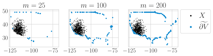
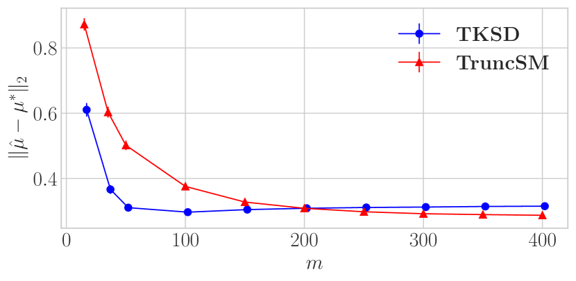
Figure 1: Density estimation when the truncation boundary is the border of the U.S., as described in Section 6.2. Top: example of increasing the number of boundary points $m$. Bottom: across 256 seeds for each value of $m$, mean estimation error with standard error bars for the mean of a 2D Gaussian, for TKSD and TruncSM as $m$ increases.

Let us consider the complicated boundary of the United States (U.S.). Let $V$ be the interior of the U.S. and let $\widetilde{\partial V}$ be a set of coordinates (longitude and latitude) which define the country’s borders. The boundary of the U.S. is a highly irregular shape, and as such, there is no explicit expression of the boundary in this case. TruncSM and bd-KSD must use an approximate distance function (given by (28)), whereas TKSD can readily use the set of coordinates that give rise to the boundary.

The experiment is set up as follows. Let $\boldsymbol{\mu}^{\star}=[-115,35]$ and $\boldsymbol{\Sigma}=10\cdot I_{d}$. Samples are simulated from $\mathcal{N}(\boldsymbol{\mu}^{\star},\boldsymbol{\Sigma})$ and we select only those which are in the interior of the U.S. until we reach $n=400$ points. Assuming $\boldsymbol{\Sigma}$ is known, we estimate $\boldsymbol{\mu}^{\star}$ with $\boldsymbol{\hat{\mu}}$ using TKSD and compare it to the estimation using TruncSM. We also vary $m$ by uniformly sampling from the perimeter of the U.S., demonstrated in Figure 1 (top).

Figure 1 (bottom) shows the mean and standard error of the $\ell_{2}$ estimation error between $\boldsymbol{\mu}^{\star}$ and $\boldsymbol{\hat{\mu}}$, measured over 256 trials for each value of $m$. TruncSM improves with higher values of $m$ as the approximate distance function increases in accuracy, whilst TKSD performs significantly better with fewer boundary points.

6.3 Estimation Error and Dimensionality

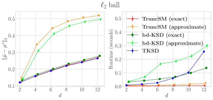
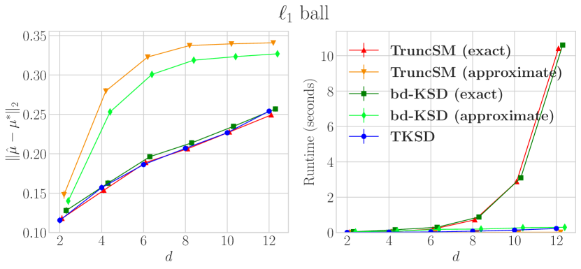
Figure 2: Mean estimation error across 256 seeds, with standard error bars, as dimension $d$ increases (left) and runtime for each method (right). The truncation domain is the $\ell_{2}$ ball of radius $d^{0.53}$ (top) and $\ell_{1}$ ball of radius $d$ (bottom).

Consider a simple experiment setup where $\boldsymbol{\mu}_{d}^{\star}=\boldsymbol{1}_{d}\cdot 0.5$, samples are simulated from $\mathcal{N}(\boldsymbol{\mu}_{d}^{\star},\boldsymbol{I}_{d})$ and are truncated be within the $\ell_{c}$ ball for $c=1$ and $c=2$, each of radius $r$, until we reach $n=300$ data points. We choose radii $r=d^{0.53}$ for $c=1$ and $r=d$ for $c=2$, chosen so that the amount of points truncated across dimension is roughly 50% (see Section B.7 for details). We estimate $\boldsymbol{\mu}_{d}^{\star}$ with $\boldsymbol{\hat{\mu}}$, and measure the $\ell_{2}$ estimation error against $\boldsymbol{\mu}_{d}^{\star}$ as $d$ increases. Each boundary point $\boldsymbol{x}^{\prime}\in\widetilde{\partial V}$ is simulated from $\mathcal{N}(\boldsymbol{0}_{d},\boldsymbol{I}_{d})$, normalized by $\|\boldsymbol{x}^{\prime}\|_{c}$, and multiplied by $r$, resulting in a set of random points on the boundary.

Figure 2 shows the error and computation time for the following estimators:

• TKSD: our method as described in Section 5, using a randomly sampled $\widetilde{\partial V}$.

• TruncSM/bd-KSD (exact): the implementation by Liu et al. (2022)/Xu (2022) respectively, where the distance function is computed exactly using the known boundaries.

• TruncSM/bd-KSD (approximate): the implementation by Liu et al. (2022)/Xu (2022) respectively with distance function given by (28), using the same $\widetilde{\partial V}$ as given to TKSD.

For the $\ell_{2}$ case, TKSD marginally outperforms all competitors across all dimensions, at only a slight computational expense. For the $\ell_{1}$ case, TKSD, bd-KSD and TruncSM have similar estimation errors across all dimensions. However, TruncSM (exact) and bd-KSD (exact) have an increasing computation time due to the costly evaluation of the distance function. In this implementation, we follow the advice of Liu et al. (2022), Section 7, where the distance function to the $\ell_{1}$ ball is calculated via a closed-form expression, for which the computational complexity increases combinatorically with dimension.

TruncSM (approximate) and bd-KSD (approximate) have significantly higher estimation error than other methods across all benchmarks. TKSD is able to achieve the same level of accuracy as the exact methods, using the same finite set of boundary points, $\widetilde{\partial V}$.

7 Discussion

We have proposed an alternative to the classical Stein class, called an approximate Stein class, bounded by a decreasing sequence instead of being strictly equal to zero. By maximising the KSD objective over this approximate Stein class, we have constructed a truncated density estimator based on KSD, called truncated KSD (TKSD), and shown that it is consistent. TKSD has advantages over the prior works by Xu (2022) and Liu et al. (2022), as it does not require a functional form of a boundary.

Some limitations of this method include the requirement of selecting hyperparameters, such as the kernel function $k$ and its associated hyperparameters, and the number of samples from the boundary, $m$. Choice of $m$ may depend on applications. Still, a larger value is preferred when the complexity of the truncation boundary is higher, or the dimension increases. However, even with the heuristic approaches presented in this paper, TKSD provides competitive results.

In experimental results, we have shown that even though we assume no access to a functional form of the boundary, TKSD performs similarly to previous methods which require the boundary to be computed. In some scenarios, TKSD performs better than these methods, or takes less time to achieve the same result.

Reproducibility

All results in this paper can be reproduced using the GitHub repository located at https://github.com/dannyjameswilliams/tksd.

Appendix A Proofs and Additional Theoretical Results

A.1 Latent Variable Approximate Stein Identity

Suppose $\boldsymbol{g}\in\mathcal{G}^{d}$, the product RKHS with $d$ elements, and the score function defined as in (13). Then Stein’s identity with this score function is written as

$$\mathbb{E}_{q}[\mathcal{T}_{q}\boldsymbol{g}(\boldsymbol{x})]=\mathbb{E}_{q}[\boldsymbol{\psi}_{q}(\boldsymbol{x})\boldsymbol{g}(\boldsymbol{x})+\boldsymbol{\nabla}_{\boldsymbol{x}}\boldsymbol{g}(\boldsymbol{x})]=\mathbb{E}_{q}[\mathbb{E}_{q(\boldsymbol{z}|\boldsymbol{x})}[\boldsymbol{\psi}_{q}(\boldsymbol{x}|\boldsymbol{z})]\boldsymbol{g}(\boldsymbol{x})+\boldsymbol{\nabla}_{\boldsymbol{x}}\boldsymbol{g}(\boldsymbol{x})].$$

Further assume the Monte Carlo estimation of

$$\mathbb{E}_{q(\boldsymbol{z}|\boldsymbol{x})}[\boldsymbol{\psi}_{q}(\boldsymbol{x}|\boldsymbol{z})]=\frac{1}{m}\sum^{m}_{i=1}\boldsymbol{\psi}_{q}(\boldsymbol{x}|\boldsymbol{z}_{i})+O_{P}(\varepsilon_{m}),$$

where $O_{P}(\varepsilon_{m})$ denotes the error term from the Monte Carlo approximation, which decreases as the number of samples, $m$, increases. Substituting this into the equation above gives

$$\mathbb{E}_{q}[\mathcal{T}_{q}\boldsymbol{g}(\boldsymbol{x})] =\mathbb{E}_{q}\left[\left(\frac{1}{m}\sum^{m}_{i=1}\boldsymbol{\psi}_{q}(\boldsymbol{x}|\boldsymbol{z}_{i})\right)\boldsymbol{g}(\boldsymbol{x})+\boldsymbol{\nabla}_{\boldsymbol{x}}\boldsymbol{g}(\boldsymbol{x})\right]+\mathbb{E}_{q}[O_{P}(\varepsilon_{m})\boldsymbol{g}(\boldsymbol{x})]$$

$$=\mathbb{E}_{q}\left[\left(\frac{1}{m}\sum^{m}_{i=1}\boldsymbol{\psi}_{q}(\boldsymbol{x}|\boldsymbol{z}_{i})\right)\boldsymbol{g}(\boldsymbol{x})+\boldsymbol{\nabla}_{\boldsymbol{x}}\boldsymbol{g}(\boldsymbol{x})\right]+O_{P}(\varepsilon_{m})$$

$$=O_{P}(\varepsilon_{m})$$

where the last equality follows from the fact that the error in the Monte Carlo approximation is accounted for by the $O_{P}(\varepsilon_{m})$ term, therefore $\frac{1}{m}\sum^{m}_{i=1}\boldsymbol{\psi}_{q}(\boldsymbol{x}|\boldsymbol{z}_{i})$ is exactly the score function $\boldsymbol{\psi}_{q}(\boldsymbol{x})$, not including approximation error. The remainder then follows by definition of $\mathcal{G}^{d}$ being a Stein class.

A.2 Proof of Lemma 5.1

Let $\boldsymbol{g}\in\mathcal{G}^{d}_{0}$. Begin by writing the expectation as an integral,

$$\mathbb{E}_{q}[\mathcal{T}_{q}\boldsymbol{g}(\boldsymbol{x})]=\int_{V}q(\boldsymbol{x})\mathcal{T}_{q}\boldsymbol{g}(\boldsymbol{x})d\boldsymbol{x} =\sum^{d}_{l=1}\int_{V}q(\boldsymbol{x})\partial_{x_{l}}\log q(\boldsymbol{x})g_{l}(\boldsymbol{x})+\partial_{x_{l}}g_{l}(\boldsymbol{x})d\boldsymbol{x}$$

$$=\sum^{d}_{l=1}\int_{V}\partial_{x_{l}}q(\boldsymbol{x})g_{l}(\boldsymbol{x})+\partial_{x_{l}}g_{l}(\boldsymbol{x})d\boldsymbol{x}.$$

This can be expanded by integration by parts,

$$\sum^{d}_{l=1}\int_{V}\partial_{x_{l}}q(\boldsymbol{x})g_{l}(\boldsymbol{x})+\partial_{x_{l}}g_{l}(\boldsymbol{x})d\boldsymbol{x} =\sum^{d}_{l=1}\oint_{\partial V}q(\boldsymbol{x})g_{l}(\boldsymbol{x})\hat{\mathrm{u}}_{l}(\boldsymbol{x})ds+\sum^{d}_{l=1}\int_{V}q(\boldsymbol{x})(\partial_{x_{l}}g_{l}(\boldsymbol{x})-\partial_{x_{l}}g_{l}(\boldsymbol{x}))d\boldsymbol{x}$$

$$=\sum^{d}_{l=1}\oint_{\partial V}q(\boldsymbol{x})g_{l}(\boldsymbol{x})\hat{\mathrm{u}}_{l}(\boldsymbol{x})ds=0,$$

where the final equality comes from all evaluations $g_{l}(\boldsymbol{x}^{\prime})=0\;\forall\boldsymbol{x}^{\prime}\in\partial V$.

A.3 Proof of Lemma 5.2.

Let $\boldsymbol{g}\in\mathcal{G}^{d}_{0}$ and $\tilde{\boldsymbol{g}}\in\mathcal{G}^{d}_{0,m}$. First note that $\boldsymbol{g}$ and $\tilde{\boldsymbol{g}}$ agree on $\widetilde{\partial V}$, i.e.

$$g_{l}(\boldsymbol{\tilde{x}}^{\prime})=\tilde{g}_{l}(\boldsymbol{\tilde{x}}^{\prime}),\;\;\forall l=1,\dots,d$$ (29)

for all $\boldsymbol{\tilde{x}}^{\prime}\in\widetilde{\partial V}$, since all $\boldsymbol{\tilde{x}}^{\prime}$ are elements of $\partial V$ also, as $\widetilde{\partial V}\subset\partial V$. First, we note that since $g_{l}$ and $\tilde{g}_{l}$ are both Lipschitz continuous, then

$$|g_{l}(\boldsymbol{x}^{\prime})-g_{l}(\boldsymbol{\tilde{x}}^{\prime})| \leq C_{1}\|\boldsymbol{x}^{\prime}-\boldsymbol{\tilde{x}}^{\prime}\|\leq C_{1}\varepsilon_{m}$$ (30)

$$|\tilde{g}_{l}(\boldsymbol{\tilde{x}}^{\prime})-\tilde{g}_{l}(\boldsymbol{x}^{\prime})| \leq C_{2}\|\boldsymbol{x}^{\prime}-\boldsymbol{\tilde{x}}^{\prime}\|\leq C_{2}\varepsilon_{m},$$ (31)

where $\|\boldsymbol{x}^{\prime}-\boldsymbol{\tilde{x}}^{\prime}\|\leq\varepsilon_{m}$. This follows under the assumption that $\widetilde{\partial V}$ is $\varepsilon_{m}$-dense in $\partial V$, therefore the distance $\|\boldsymbol{x}^{\prime}-\boldsymbol{\tilde{x}}^{\prime}\|$ is at most $\varepsilon_{m}$.

We seek to quantify

$$|g_{l}(\boldsymbol{x}^{\prime})-\tilde{g}_{l}(\boldsymbol{x}^{\prime})|,$$

which is how far apart the ‘approximate’ $\tilde{g}_{l}$ is from the ‘true’ $g_{l}$ for any point $\boldsymbol{x}^{\prime}\in\partial V$. Note that this includes points that are not in $\widetilde{\partial V}$. We let

$$g_{l}(\boldsymbol{x}^{\prime})-\tilde{g}_{l}(\boldsymbol{x}^{\prime})=(g_{l}(\boldsymbol{x}^{\prime})-\tilde{g}_{l}(\boldsymbol{x}^{\prime}))+(g_{l}(\boldsymbol{\tilde{x}}^{\prime})-g_{l}(\boldsymbol{\tilde{x}}^{\prime}))+(\tilde{g}_{l}(\boldsymbol{\tilde{x}}^{\prime})-\tilde{g}_{l}(\boldsymbol{\tilde{x}}^{\prime})),$$

and by (29),

$$g_{l}(\boldsymbol{x}^{\prime})-\tilde{g}_{l}(\boldsymbol{x}^{\prime}) =(g_{l}(\boldsymbol{x}^{\prime})-\tilde{g}_{l}(\boldsymbol{x}^{\prime}))-g_{l}(\boldsymbol{\tilde{x}}^{\prime})+\tilde{g}_{l}(\boldsymbol{\tilde{x}}^{\prime})$$

$$=(g_{l}(\boldsymbol{x}^{\prime})-g_{l}(\boldsymbol{\tilde{x}}^{\prime}))+(\tilde{g}_{l}(\boldsymbol{\tilde{x}}^{\prime})-\tilde{g}_{l}(\boldsymbol{x}^{\prime})).$$

Using (30) and (31), we have the following inequality,

$$|g_{l}(\boldsymbol{x}^{\prime})-\tilde{g}_{l}(\boldsymbol{x}^{\prime})|\leq|g_{l}(\boldsymbol{x}^{\prime})-g_{l}(\boldsymbol{\tilde{x}}^{\prime})|+|\tilde{g}_{l}(\boldsymbol{\tilde{x}}^{\prime})-\tilde{g}_{l}(\boldsymbol{x}^{\prime})|\leq(C_{1}+C_{2})\varepsilon_{m},$$

where the last step follows by the triangle inequality. Therefore, we have

$$|g_{l}(\boldsymbol{x}^{\prime})-\tilde{g}_{l}(\boldsymbol{x}^{\prime})|=O_{P}(\varepsilon_{m})$$

as desired.

A.4 Proof of Proposition 5.3

First, let $\mathrm{L}(V)$ denote the $(d-1)$-surface area of a bounded domain $V\subset\mathbb{R}^{d}$ and $\mathrm{L}(V)<\infty$. For example, in 2D, $\mathrm{L}(V)$ corresponds to the line length of $\partial V$. We also define $B_{\varepsilon_{m}}(\boldsymbol{x}^{\prime})$ as the ball of radius $\varepsilon_{m}$ centred on $\boldsymbol{x}^{\prime}$.

Before continuing to the proof, recall the definition of an $\varepsilon$-dense set: $\forall\boldsymbol{x}^{\prime}\in\partial V,\exists\hskip 1.42262pt\widetilde{\boldsymbol{x}}^{\prime}\in\widetilde{\partial V}$ such that $d(\boldsymbol{x}^{\prime},\widetilde{\boldsymbol{x}}^{\prime})\leq\varepsilon$, where $d$ is some measure of distance. The statement $d(\boldsymbol{x}^{\prime},\widetilde{\boldsymbol{x}}^{\prime})\leq\varepsilon_{m}$ is equivalent to $\widetilde{\boldsymbol{x}}^{\prime}\in B_{\varepsilon_{m}}(\boldsymbol{x}^{\prime})$. Now write that the probability that the definition of a $\varepsilon_{m}$-dense set holds for $\widetilde{\partial V}$ being dense in $\partial V$ is equal to 0.95:

$$0.95=\mathbb{P}(\exists\hskip 1.42262pt\widetilde{\boldsymbol{x}}^{\prime}\in\widetilde{\partial V},\widetilde{\boldsymbol{x}}^{\prime}\in B_{\varepsilon_{m}}(\boldsymbol{x}^{\prime}),\forall\boldsymbol{x}^{\prime}\in\partial V) =1-\mathbb{P}(\exists\hskip 1.42262pt\boldsymbol{x}^{\prime}\in\partial V,\forall\widetilde{\boldsymbol{x}}^{\prime}\in\widetilde{\partial V},\widetilde{\boldsymbol{x}}^{\prime}\notin B_{\varepsilon_{m}}(\boldsymbol{x}^{\prime}))$$

$$=1-\mathbb{P}\Big{(}\bigcup_{\boldsymbol{x}^{\prime}\in\partial V}\forall\widetilde{\boldsymbol{x}}^{\prime}\in\widetilde{\partial V},\widetilde{\boldsymbol{x}}^{\prime}\notin B_{\varepsilon_{m}}(\boldsymbol{x}^{\prime})\Big{)}.$$

Equivalently, by rearranging the above, we have

$$\mathbb{P}\Big{(}\bigcup_{\boldsymbol{x}^{\prime}\in\partial V}\forall\widetilde{\boldsymbol{x}}^{\prime}\in\widetilde{\partial V},\widetilde{\boldsymbol{x}}^{\prime}\notin B_{\varepsilon_{m}}(\boldsymbol{x}^{\prime})\Big{)}=0.05.$$

Note the definition of the union bound: $\mathbb{P}(\bigcup_{i=1}^{\infty}E_{i})\leq\sum^{\infty}_{i=1}\mathbb{P}(E_{i})$, where $E_{i}$ are a collection of events. Using this, we can write

$$\mathbb{P}\Big{(}\bigcup_{\boldsymbol{x}^{\prime}\in\partial V}\forall\widetilde{\boldsymbol{x}}^{\prime}\in\widetilde{\partial V},\widetilde{\boldsymbol{x}}^{\prime}\notin B_{\varepsilon_{m}}(\boldsymbol{x}^{\prime})\Big{)}\leq\sum_{\boldsymbol{x}^{\prime}\in\partial V}\mathbb{P}\left(\forall\widetilde{\boldsymbol{x}}^{\prime}\in\widetilde{\partial V},\widetilde{\boldsymbol{x}}^{\prime}\notin B_{\varepsilon_{m}}(\boldsymbol{x}^{\prime})\right)$$ (32)

Next, consider a set $A\subseteq\partial V$ such that for all $\boldsymbol{x}^{\prime}\in A$, $A$ is the smallest set that satisfies

$$\bigcup_{\boldsymbol{x}^{\prime}\in A}B_{\varepsilon_{m}}(\boldsymbol{x}^{\prime})\cap\partial V=\partial V,$$

i.e. $A$ defines the set of all $\boldsymbol{x}^{\prime}$ such that the smallest number of $\varepsilon_{m}$-balls centred on $\boldsymbol{x}^{\prime}$ cover $\partial V$. Let $n_{\varepsilon_{m}}=|A|$. Using $A$, the following equivalence holds

$$\sum_{\boldsymbol{x}^{\prime}\in\partial V}\mathbb{P}\left(\forall\widetilde{\boldsymbol{x}}^{\prime}\in\widetilde{\partial V},\widetilde{\boldsymbol{x}}^{\prime}\notin B_{\varepsilon_{m}}(\boldsymbol{x}^{\prime})\right)=\sum_{\boldsymbol{x}^{\prime}\in A}\mathbb{P}\left(\forall\widetilde{\boldsymbol{x}}^{\prime}\in\widetilde{\partial V},\widetilde{\boldsymbol{x}}^{\prime}\notin B_{\varepsilon_{m}}(\boldsymbol{x}^{\prime})\right).$$ (33)

Consider a given $\boldsymbol{x}^{\prime}_{0}\in\partial V$ and $\widetilde{\boldsymbol{x}}^{\prime}_{0}\in\widetilde{\partial V}$. The above equality holds due to only needing to consider all $\boldsymbol{x}^{\prime}\in\partial V$ such that $\boldsymbol{x}^{\prime}\notin B_{\varepsilon_{m}}(\boldsymbol{x}^{\prime}_{0})$, because by definition, if $\boldsymbol{x}^{\prime}\in B_{\varepsilon_{m}}(\boldsymbol{x}^{\prime}_{0})$, then $\widetilde{\boldsymbol{x}}^{\prime}\in B_{\varepsilon_{m}}(\boldsymbol{x}^{\prime})$ also. Note that the probability inside the sum in (33) is equal for any independent realisations $\widetilde{\boldsymbol{x}}^{\prime}\in\widetilde{\partial V}$ and $\boldsymbol{x}^{\prime}\in A$, and can be re-written as

$$\sum_{\boldsymbol{x}^{\prime}\in A}\mathbb{P}\left(\forall\widetilde{\boldsymbol{x}}^{\prime}\in\widetilde{\partial V},\widetilde{\boldsymbol{x}}^{\prime}\notin B_{\varepsilon_{m}}(\boldsymbol{x}^{\prime}_{0})\right) =n_{\varepsilon_{m}}\left[\mathbb{P}\left(\widetilde{\boldsymbol{x}}^{\prime}_{0}\notin B_{\varepsilon_{m}}(\boldsymbol{x}^{\prime}_{0})\right)\right]^{m}$$

$$=n_{\varepsilon_{m}}\left[1-\mathbb{P}\left(\widetilde{\boldsymbol{x}}^{\prime}_{0}\in B_{\varepsilon_{m}}(\boldsymbol{x}^{\prime}_{0})\right)\right]^{m}$$

$$=n_{\varepsilon_{m}}\left[1-\frac{\mathrm{Area}(\partial V\cap B_{\varepsilon_{m}}(\boldsymbol{x}^{\prime}_{0}))}{\mathrm{L}(V)}\right]^{m}\geq 0.05$$ (34)

Where $\mathrm{Area}(S)$ denotes the surface area of the boundary set $S$. For example, $\mathrm{Area}(\partial V)=\mathrm{L}(V)$. Therefore $\mathrm{Area}(\partial V\cap B_{\varepsilon_{m}}(\boldsymbol{x}^{\prime}_{0}))$ represents the size of the region of $\partial V$ that is inside $B_{\varepsilon_{m}}(\boldsymbol{x}^{\prime}_{0})$, which will be the area of the boundary hyperplane of $\partial V$ which passes through $B_{\varepsilon_{m}}(\boldsymbol{x}^{\prime}_{0})$. We obtain the probability in the final equality by assuming that all$\widetilde{\boldsymbol{x}}^{\prime}$ are uniformly sampled from $\partial V$, so the probability is the proportion of $\partial V$ inside $B_{\varepsilon_{m}}(\boldsymbol{x}^{\prime}_{0})$ as a ratio of the full $\partial V$. This probability exists under the assumption that $\mathrm{L}(V)<\infty$. Now we can rearrange (34) to obtain

$$\mathrm{Area}(\partial V\cap B_{\varepsilon_{m}}(\boldsymbol{x}^{\prime}_{0}))\leq\mathrm{L}(V)\left[1-\left(\frac{0.05}{n_{\varepsilon_{m}}}\right)^{1/m}\right]\leq\xi(d)\varepsilon_{m}^{d},$$

where we have used the following bound,

$$\mathrm{Area}(\partial V\cap B_{\varepsilon}(\boldsymbol{x}^{\prime}_{0}))\leq\xi(d)\varepsilon_{m}^{d},\qquad\xi(d)=\frac{\pi^{d/2}}{\Gamma(\frac{d}{2}+1)},$$

i.e. the intersection between $\partial V$ and $B_{\varepsilon_{m}}(\boldsymbol{x}^{\prime})$ is at most the volume of the ball $B_{\varepsilon_{m}}(\boldsymbol{x}^{\prime})$. Rearranging for $\varepsilon_{m}$, we obtain

$$\varepsilon_{m}\leq\left(\frac{\mathrm{L}(V)}{\xi(d)}\left[1-\left(\frac{0.05}{n_{\varepsilon_{m}}}\right)^{1/m}\right]\right)^{1/d},$$

as desired.

A.5 Proof of Theorem 5.5

Let $\boldsymbol{g}\in\mathcal{G}^{d}_{0}$ and $\tilde{\boldsymbol{g}}\in\mathcal{G}^{d}_{0,m}$. Begin with writing the expectation in its integral form,

$$\mathbb{E}_{q}[\mathcal{T}_{q}\tilde{\boldsymbol{g}}(\boldsymbol{x})] =\int_{V}q(\boldsymbol{x})\left[\sum_{l=1}^{d}\partial_{x_{l}}\log q(\boldsymbol{x})\tilde{g}_{l}(\boldsymbol{x})+\sum_{l=1}^{d}\partial_{x_{l}}\tilde{g}_{l}(\boldsymbol{x})\right]d\boldsymbol{x}$$

$$=\sum_{l=1}^{d}\int_{V}q(\boldsymbol{x})\partial_{x_{l}}\log q(\boldsymbol{x})\tilde{g}_{l}(\boldsymbol{x})d\boldsymbol{x}+\sum_{l=1}^{d}\int_{V}q(\boldsymbol{x})\partial_{x_{l}}\tilde{g}_{l}(\boldsymbol{x})d\boldsymbol{x}$$

$$\stackrel{{\scriptstyle\mathclap{\tiny\mbox{(a)}}}}{{=}}\sum_{l=1}^{d}\int_{V}\partial_{x_{l}}q(\boldsymbol{x})\tilde{g}_{l}(\boldsymbol{x})d\boldsymbol{x}+\sum_{l=1}^{d}\int_{V}q(\boldsymbol{x})\partial_{x_{l}}\tilde{g}_{l}(\boldsymbol{x})d\boldsymbol{x}$$

$$\stackrel{{\scriptstyle\mathclap{\tiny\mbox{(b)}}}}{{=}}\sum_{l=1}^{d}\oint_{\partial V}q(\boldsymbol{x})\tilde{g}_{l}(\boldsymbol{x})\hat{\mathrm{u}}_{l}(\boldsymbol{x})ds-\sum_{l=1}^{d}\int_{V}q(\boldsymbol{x})\partial_{x_{l}}\tilde{g}_{l}(\boldsymbol{x})d\boldsymbol{x}+\sum_{l=1}^{d}\int_{V}q(\boldsymbol{x})\partial_{x_{l}}\tilde{g}_{l}(\boldsymbol{x})d\boldsymbol{x}$$

$$=\sum_{l=1}^{d}\oint_{\partial V}q(\boldsymbol{x})\tilde{g}_{l}(\boldsymbol{x})\hat{\mathrm{u}}_{l}(\boldsymbol{x})ds$$

where $\oint_{\partial V}$ is the surface integral over the boundary $\partial V$, (a) comes from the identity that $q(\boldsymbol{x})\partial_{x_{l}}\log q(\boldsymbol{x})=\partial_{x_{l}}q(\boldsymbol{x})$, and (b) is from integration by parts. Substitute $\tilde{g}_{l}(\boldsymbol{x})=\tilde{g}_{l}(\boldsymbol{x})+g_{l}(\boldsymbol{x})-g_{l}(\boldsymbol{x})$ to obtain

$$\sum_{l=1}^{d}\oint_{\partial V}q(\boldsymbol{x})(\tilde{g}_{l}(\boldsymbol{x})+g_{l}(\boldsymbol{x})-g_{l}(\boldsymbol{x}))\hat{\mathrm{u}}_{l}(\boldsymbol{x})ds$$

$$= \sum_{l=1}^{d}\oint_{\partial V}q(\boldsymbol{x})(\tilde{g}_{l}(\boldsymbol{x})-g_{l}(\boldsymbol{x}))\hat{\mathrm{u}}_{l}(\boldsymbol{x})ds+\sum_{l=1}^{d}\oint_{\partial V}q(\boldsymbol{x})g_{l}(\boldsymbol{x})\hat{\mathrm{u}}_{l}(\boldsymbol{x})ds.$$

By Lemma 5.2, $|\tilde{g}_{l}(\boldsymbol{x}^{\prime})-g_{l}(\boldsymbol{x}^{\prime})|=O_{P}(\varepsilon_{m})$, leaving

$$\mathbb{E}_{q}[\mathcal{T}_{q}\tilde{\boldsymbol{g}}(\boldsymbol{x})]=O_{P}(\varepsilon_{m})+\sum_{l=1}^{d}\oint_{\partial V}q(\boldsymbol{x})g_{l}(\boldsymbol{x})\hat{\mathrm{u}}_{l}(\boldsymbol{x})ds$$

As all evaluations of $g_{l}(\boldsymbol{x})=0\;\forall\boldsymbol{x}\in\partial V$ by definition of $\mathcal{G}^{d}_{0}$, the second term equals zero, leaving only

$$\mathbb{E}_{q}[\mathcal{T}_{q}\tilde{\boldsymbol{g}}(\boldsymbol{x})]=O_{P}(\varepsilon_{m})$$

as desired.

A.6 Proof of Theorem 5.6

Recall $\mathcal{G}^{d}_{0,m}=\{\boldsymbol{g}\in\mathcal{G}^{d}\;|\;\boldsymbol{g}(\boldsymbol{x}^{\prime})=\boldsymbol{0}\>\forall\boldsymbol{x}^{\prime}\in\widetilde{\partial V},\|\boldsymbol{g}\|^{2}_{\mathcal{G}^{d}}\leq 1\}$, where $\mathcal{G}^{d}$ is the product RKHS with $d$ elements, $\boldsymbol{g}=(g_{1},\dots,g_{d})$, and $g_{l}\in\mathcal{G},\forall l=1,\dots,d$.

Begin with the definition of TKSD as defined in (21),

$$\sup_{\boldsymbol{g}\in\mathcal{G}^{d}_{0,m}}\mathbb{E}_{q}[\mathcal{T}_{p_{\boldsymbol{\theta}}}\boldsymbol{g}(\boldsymbol{x})].$$

To solve this supremum analytically, we can reframe it as a constrained maximisation problem,

$$\max_{\boldsymbol{g}\in\mathcal{G}^{d}}\> \mathbb{E}_{q}[\mathcal{T}_{p_{\boldsymbol{\theta}}}\boldsymbol{g}(\boldsymbol{x})],$$ (35)

subject to $$g_{l}(\boldsymbol{x}^{\prime})=0\;\forall\boldsymbol{x}^{\prime}\in\widetilde{\partial V},\;\forall l=1,\dots,d$$

$$\|\boldsymbol{g}\|_{\mathcal{G}^{d}}\leq 1,$$

where the constraints in the definition for $\mathcal{G}^{d}_{0,m}$ have been included as optimisation constraints, and the maximisation is now with respect to the RKHS function family $\mathcal{G}^{d}$ only. To solve this, we can formulate a Lagrangian dual function (Boyd & Vandenberghe, 2004).

$$\inf_{\boldsymbol{\nu}^{(1)},\dots,\boldsymbol{\nu}^{(d)},\lambda} \mathcal{L}(\boldsymbol{\theta},\boldsymbol{g},\boldsymbol{\nu}^{(1)},\dots,\boldsymbol{\nu}^{(d)},\lambda)$$ (36)

$$\mathcal{L}=\mathcal{L}(\boldsymbol{\theta},\boldsymbol{g},\boldsymbol{\nu}^{(1)},\dots,\boldsymbol{\nu}^{(d)},\lambda):=\; \mathbb{E}_{q}[\mathcal{T}_{p_{\boldsymbol{\theta}}}\boldsymbol{g}(\boldsymbol{x})]+\sum^{d}_{l=1}\sum^{m}_{i^{\prime}=1}\nu^{(l)}_{i^{\prime}}g_{l}(\boldsymbol{x}^{\prime}_{i^{\prime}})+\lambda(\|\boldsymbol{g}\|^{2}_{\mathcal{G}^{d}}-1),$$ (37)

for $\boldsymbol{\nu}^{(l)}\in\mathbb{R}^{m}\;\forall l$, $\lambda\geq 0$ and $\mathcal{L}$ is our Lagrangian. The overall optimisation problem that needs solving is given by

$$\min_{\boldsymbol{\nu}^{(1)},\dots,\boldsymbol{\nu}^{(d)},\lambda}\;\;\max_{\boldsymbol{g}\in\mathcal{G}^{d}}\;\mathcal{L}(\boldsymbol{\theta},\boldsymbol{g},\boldsymbol{\nu}^{(1)},\dots,\boldsymbol{\nu}^{(d)},\lambda).$$ (38)

By solving the dual problem, (38), we solve the primal problem, (35). We can rewrite (37) as

$$\mathcal{L}=\mathbb{E}_{q}\left[\sum^{d}_{l=1}\partial_{x_{l}}\log p_{\boldsymbol{\theta}}(\boldsymbol{x})g_{l}(\boldsymbol{x})+\partial_{x_{l}}g_{l}(\boldsymbol{x})\right]+\sum^{d}_{l=1}\sum^{m}_{i^{\prime}=1}\nu^{(l)}_{i^{\prime}}g_{l}(\boldsymbol{x}^{\prime}_{i^{\prime}})+\lambda(\|\boldsymbol{g}\|^{2}_{\mathcal{G}^{d}}-1),$$

and expand evaluations of $g_{l}(\boldsymbol{x})$ via the reproducing property of $\mathcal{G}$, given by $g_{l}(\boldsymbol{x})=\langle g_{l},k(\boldsymbol{x},\cdot)\rangle_{\mathcal{G}}$, to

$$\mathcal{L} =\mathbb{E}_{q}\left[\sum^{d}_{l=1}\partial_{x_{l}}\log p_{\boldsymbol{\theta}}(\boldsymbol{x})\left\langle g_{l},k(\boldsymbol{x},\cdot)\right\rangle_{\mathcal{G}}+\left\langle g_{l},\partial_{x_{l}}k(\boldsymbol{x},\cdot)\right\rangle_{\mathcal{G}}\right]+\sum^{m}_{i^{\prime}=1}\sum^{d}_{i=1}\nu^{(l)}_{i^{\prime}}\left\langle g_{l},k(\boldsymbol{x}^{\prime}_{i^{\prime}},\cdot)\right\rangle_{\mathcal{G}}+\lambda\left(\sum^{d}_{l=1}\langle g_{l},g_{l}\rangle_{\mathcal{G}}-1\right)$$

$$=\sum^{d}_{l=1}\mathbb{E}_{q}\left[\left\langle g_{l},\partial_{x_{l}}\log p_{\boldsymbol{\theta}}(\boldsymbol{x})k(\boldsymbol{x},\cdot)+\partial_{x_{l}}k(\boldsymbol{x},\cdot)+\sum^{m}_{i^{\prime}=1}\nu^{(l)}_{i^{\prime}}k(\boldsymbol{x}^{\prime}_{i^{\prime}},\cdot)\right\rangle_{\mathcal{G}}\right]+\lambda\left(\sum^{d}_{l=1}\langle g_{l},g_{l}\rangle_{\mathcal{G}}-1\right)$$

$$=\sum^{d}_{l=1}\Big{\langle}g_{l},\mathbb{E}_{q}[\partial_{x_{l}}\log p_{\boldsymbol{\theta}}(\boldsymbol{x})k(\boldsymbol{x},\cdot)+\partial_{x_{l}}k(\boldsymbol{x},\cdot)]+\sum^{m}_{i^{\prime}=1}\nu^{(l)}_{i^{\prime}}k(\boldsymbol{x}^{\prime}_{i^{\prime}},\cdot)\Big{\rangle}_{\mathcal{G}}+\lambda\left(\sum^{d}_{l=1}\langle g_{l},g_{l}\rangle_{\mathcal{G}}-1\right).$$ (39)

The final equality holds provided that $\mathbb{E}_{q}[\partial_{x_{l}}\log p_{\boldsymbol{\theta}}(\boldsymbol{x})k(\boldsymbol{x},\cdot)+\partial_{x_{l}}k(\boldsymbol{x},\cdot)+\sum^{m}_{i^{\prime}=1}\nu^{(l)}_{i^{\prime}}k(\boldsymbol{x}^{\prime}_{i^{\prime}},\cdot)]<\infty$, i.e. the term inside the expectation is Bochner integrable (Steinwart & Christmann, 2008). This same assumption was made in Chwialkowski et al. (2016), as we can consider $\sum^{m}_{i^{\prime}=1}\nu^{(l)}_{i^{\prime}}k(\boldsymbol{x}^{\prime}_{i^{\prime}},\cdot)$ as a constant with respect to the expectation.

We solve for each parameter via differentiation to obtain a closed form solution. Across dimensions, each $g_{l}$ in (39) appears only additively to another, and so we can consider the $l$-th element of the derivative, and solve the inner maximisation for each $g_{l}$ to give a solution for $\boldsymbol{g}$. This differentiation gives

$$\frac{\partial\mathcal{L}}{\partial g_{l}}=\mathbb{E}_{q}\left[\partial_{x_{l}}\log p_{\boldsymbol{\theta}}(\boldsymbol{x})k(\boldsymbol{x},\cdot)+\partial_{x_{l}}k(\boldsymbol{x},\cdot)\right]+\sum^{m}_{i^{\prime}=1}\nu^{(l)}_{i^{\prime}}k(\boldsymbol{x}^{\prime}_{i^{\prime}},\cdot)+2\lambda g_{l}=0.$$

Rearranging for $g_{l}$ gives the solution

$$g_{l}^{\star}=-\frac{1}{2\lambda}\mathbb{E}_{q}\left[\partial_{x_{l}}\log p_{\boldsymbol{\theta}}(\boldsymbol{x})k(\boldsymbol{x},\cdot)+\partial_{x_{l}}k(\boldsymbol{x},\cdot)\right]-\frac{1}{2\lambda}\sum^{m}_{i^{\prime}=1}\nu^{(l)}_{i^{\prime}}k(\boldsymbol{x}^{\prime}_{i^{\prime}},\cdot)=-\frac{z_{l}}{2\lambda},$$

where for convenience we have denoted $z_{l}=\mathbb{E}_{q}\left[\partial_{x_{l}}\log p_{\boldsymbol{\theta}}(\boldsymbol{x})k(\boldsymbol{x},\cdot)+\partial_{x_{l}}k(\boldsymbol{x},\cdot)\right]+\sum^{m}_{i^{\prime}=1}\nu^{(l)}_{i^{\prime}}k(\boldsymbol{x}^{\prime}_{i^{\prime}},\cdot)$. Substituting this back into (39) gives

$$\mathcal{L}(\boldsymbol{\theta},\boldsymbol{g}^{\star},\boldsymbol{\nu}^{(1)},\dots,\boldsymbol{\nu}^{(d)},\lambda)=\sum^{d}_{l=1}\left\langle-\frac{z_{l}}{2\lambda},z_{l}\right\rangle_{\mathcal{G}}+\lambda\left(\sum^{d}_{i=1}\left\langle-\frac{z_{l}}{2\lambda},-\frac{z_{l}}{2\lambda}\right\rangle_{\mathcal{G}}-1\right)=\sum^{d}_{l=1}\frac{1}{4\lambda}\left\langle z_{l},z_{l}\right\rangle_{\mathcal{G}}+\lambda,$$ (40)

where $\boldsymbol{g}^{\star}=(g_{1}^{\star},\dots,g_{d}^{\star})$. Solve for $\lambda$ by differentiating

$$\frac{\partial\mathcal{L}}{\partial\lambda}=-\frac{1}{4\lambda^{2}}\sum^{d}_{i=1}\left\langle z_{l},z_{l}\right\rangle_{\mathcal{G}}+1=0.$$

Rearranging for $\lambda$ gives $\lambda=\pm\sqrt{{\sum^{d}_{l=1}\left\langle z_{l},z_{l}\right\rangle_{\mathcal{G}}}/{4}}$. Since $\lambda\geq 0$, we take the positive solution, giving $\lambda^{\star}=\sqrt{\sum^{d}_{l=1}\left\langle z_{l},z_{l}\right\rangle_{\mathcal{G}}}/2$. Substituting $\lambda^{\star}$ into (40) gives

$$\mathcal{L}(\boldsymbol{\theta},\boldsymbol{g}^{\star},\boldsymbol{\nu}^{(1)},\dots,\boldsymbol{\nu}^{(d)},\lambda^{\star})=\sum^{d}_{l=1}\frac{1}{4\lambda^{\star}}\left\langle z_{l},z_{l}\right\rangle_{\mathcal{G}}+\lambda^{\star}=\sqrt{\sum^{d}_{l=1}\left\langle z_{l},z_{l}\right\rangle_{\mathcal{G}}}.$$ (41)

To solve for the final Lagrangian parameters, $\boldsymbol{\nu}^{(1)},\dots,\boldsymbol{\nu}^{(d)}$, let us first introduce some notation. Denote

$$\boldsymbol{\phi}_{\mathbf{x}^{\prime}}=\begin{bmatrix}k(\boldsymbol{x}_{1}^{\prime},\cdot),\\ \vdots,\\ k(\boldsymbol{x}_{m}^{\prime},\cdot)\end{bmatrix},\qquad\boldsymbol{\varphi}_{\boldsymbol{z},\mathbf{x}^{\prime}}=\begin{bmatrix}k(\boldsymbol{z},\boldsymbol{x}_{1}^{\prime})&\ldots&k(\boldsymbol{z},\boldsymbol{x}_{m}^{\prime})\end{bmatrix},\qquad\mathbf{K}^{\prime}=\boldsymbol{\phi}_{\mathbf{x}^{\prime}}\boldsymbol{\phi}_{\mathbf{x}^{\prime}}^{\top},$$

where $\boldsymbol{x}^{\prime}_{1},\dots,\boldsymbol{x}^{\prime}_{m}\in\widetilde{\partial V}$. Now consider the equivalence

$${\boldsymbol{\nu}^{(l)}}^{\star}:=\operatorname*{arg\,min}_{\boldsymbol{\nu}^{(l)}}\sqrt{\sum^{d}_{l=1}\left\langle z_{l},z_{l}\right\rangle_{\mathcal{G}}}=\operatorname*{arg\,min}_{\boldsymbol{\nu}^{(l)}}\sum^{d}_{l=1}\left\langle z_{l},z_{l}\right\rangle_{\mathcal{G}}=\operatorname*{arg\,min}_{\boldsymbol{\nu}^{(l)}}\left\langle z_{l},z_{l}\right\rangle_{\mathcal{G}},$$

as each $\boldsymbol{\nu}^{(l)}$ is independent. By rewriting $z_{l}$ as $z_{l}=\mathbb{E}_{q}\left[\partial_{x_{l}}\log p_{\boldsymbol{\theta}}(\boldsymbol{x})k(\boldsymbol{x},\cdot)+\partial_{x_{l}}k(\boldsymbol{x},\cdot)\right]+{\boldsymbol{\nu}^{(l)}}^{\top}\boldsymbol{\phi}_{\mathbf{x}^{\prime}},$ we solve this again by differentiating,

$$\frac{d}{d\boldsymbol{\nu}^{(l)}}\left\langle z_{l},z_{l}\right\rangle_{\mathcal{G}}=2\left\langle\frac{dz_{l}}{d\boldsymbol{\nu}^{(l)}},z_{l}\right\rangle_{\mathcal{G}} =2\left\langle\boldsymbol{\phi}_{\mathbf{x}^{\prime}},\mathbb{E}_{q}\left[\partial_{x_{l}}\log p_{\boldsymbol{\theta}}(\boldsymbol{x})k(\boldsymbol{x},\cdot)+\partial_{x_{l}}k(\boldsymbol{x},\cdot)\right]+{\boldsymbol{\nu}^{(l)}}^{\top}\boldsymbol{\phi}_{\mathbf{x}^{\prime}}\right\rangle_{\mathcal{G}}$$

$$=2\;\mathbb{E}_{q}\left[\partial_{x_{l}}\log p_{\boldsymbol{\theta}}(\boldsymbol{x})\boldsymbol{\varphi}_{\boldsymbol{x},\mathbf{x}^{\prime}}+\partial_{x_{l}}\boldsymbol{\varphi}_{\boldsymbol{x},\mathbf{x}^{\prime}}\right]+2{\boldsymbol{\nu}^{(l)}}^{\top}\boldsymbol{\phi}_{\mathbf{x}^{\prime}}\boldsymbol{\phi}_{\mathbf{x}^{\prime}}^{\top}$$

$$=2\;\mathbb{E}_{q}\left[\partial_{x_{l}}\log p_{\boldsymbol{\theta}}(\boldsymbol{x})\boldsymbol{\varphi}_{\boldsymbol{x},\mathbf{x}^{\prime}}+\partial_{x_{l}}\boldsymbol{\varphi}_{\boldsymbol{x},\mathbf{x}^{\prime}}\right]+2{\boldsymbol{\nu}^{(l)}}^{\top}\mathbf{K}^{\prime}.$$

Setting equal to zero and rearranging gives

$${\boldsymbol{\nu}^{(l)}}^{\star}=-(\mathbf{K}^{\prime})^{-1}\mathbb{E}_{q}\left[\partial_{x_{l}}\log p_{\boldsymbol{\theta}}(\boldsymbol{x})\boldsymbol{\varphi}_{\boldsymbol{x},\mathbf{x}^{\prime}}^{\top}+(\partial_{x_{l}}\boldsymbol{\varphi}_{\boldsymbol{x},\mathbf{x}^{\prime}})^{\top}\right].$$ (42)

Before substituting back into (41), let us first square it and expand it as

$$\begin{split}\mathcal{L}^{2}&=\sum^{d}_{l=1}\mathbb{E}_{\boldsymbol{x}\sim q}\mathbb{E}_{\boldsymbol{y}\sim q}[u_{l}(\boldsymbol{x},\boldsymbol{y})]+\left(\mathbb{E}_{\boldsymbol{x}\sim q}\Big{[}\partial_{x_{l}}\log p_{\boldsymbol{\theta}}(\boldsymbol{x})\boldsymbol{\varphi}_{\boldsymbol{x},\mathbf{x}^{\prime}}^{\top}+(\partial_{x_{l}}\boldsymbol{\varphi}_{\boldsymbol{x},\mathbf{x}^{\prime}})^{\top}\Big{]}\right)^{\top}\boldsymbol{\nu}^{(l)}\\ &\qquad\qquad\qquad\qquad\qquad+{\boldsymbol{\nu}^{(l)}}^{\top}\mathbb{E}_{\boldsymbol{y}\sim q}\Big{[}\partial_{y_{l}}\log p_{\boldsymbol{\theta}}(\boldsymbol{y})\boldsymbol{\varphi}_{\boldsymbol{y},\mathbf{x}^{\prime}}^{\top}+(\partial_{y_{l}}\boldsymbol{\varphi}_{\boldsymbol{y},\mathbf{x}^{\prime}})^{\top}\Big{]}+{\boldsymbol{\nu}^{(l)}}^{\top}\mathbf{K}^{\prime}{\boldsymbol{\nu}^{(l)}}\end{split}$$ (43)

where $u_{l}(\boldsymbol{x},\boldsymbol{y})=\psi_{p,l}(\boldsymbol{x})\psi_{p,l}(\boldsymbol{y})k(\boldsymbol{x},\boldsymbol{y})+\psi_{p,l}(\boldsymbol{x})\partial_{y_{l}}k(\boldsymbol{x},\boldsymbol{y})+\psi_{p,l}(\boldsymbol{y})\partial_{x_{l}}k(\boldsymbol{x},\boldsymbol{y})+\partial_{x_{l}}\partial_{y_{l}}k(\boldsymbol{x},\boldsymbol{y}).$ We can substitute ${\boldsymbol{\nu}^{(l)}}^{\star}$ from (42) into $\mathcal{L}^{2}$, denoting ${\mathcal{L}^{\star}}^{2}:=\mathcal{L}(\boldsymbol{\theta},\boldsymbol{g}^{\star},{\boldsymbol{\nu}^{(1)}}^{\star},\dots,{\boldsymbol{\nu}^{(d)}}^{\star},\lambda)$, giving

$$\mathcal{L}^{2} =\sum^{d}_{l=1}\mathbb{E}_{\boldsymbol{x}\sim q}\mathbb{E}_{\boldsymbol{y}\sim q}[u_{l}(\boldsymbol{x},\boldsymbol{y})]+\left(\mathbb{E}_{\boldsymbol{x}\sim q}\Big{[}\psi_{\boldsymbol{x},l}\boldsymbol{\varphi}_{\boldsymbol{x},\mathbf{x}^{\prime}}^{\top}+(\partial_{x_{l}}\boldsymbol{\varphi}_{\boldsymbol{x},\mathbf{x}^{\prime}})^{\top}\Big{]}\right)^{\top}\left(-(\mathbf{K}^{\prime})^{-1}\mathbb{E}_{\boldsymbol{y}\sim q}\Big{[}\psi_{\boldsymbol{y},l}\boldsymbol{\varphi}_{\boldsymbol{y},\mathbf{x}^{\prime}}^{\top}+(\partial_{y_{l}}\boldsymbol{\varphi}_{\boldsymbol{y},\mathbf{x}^{\prime}})^{\top}\Big{]}\right)$$

$$\qquad\qquad+\left(-(\mathbf{K}^{\prime})^{-1}\mathbb{E}_{\boldsymbol{x}\sim q}\left[\psi_{\boldsymbol{x},l}\boldsymbol{\varphi}_{\boldsymbol{x},\mathbf{x}^{\prime}}^{\top}+(\partial_{x_{l}}\boldsymbol{\varphi}_{\boldsymbol{x},\mathbf{x}^{\prime}})^{\top}\right]\right)^{\top}\mathbb{E}_{\boldsymbol{y}\sim q}\Big{[}\psi_{\boldsymbol{y},l}\boldsymbol{\varphi}_{\boldsymbol{y},\mathbf{x}^{\prime}}^{\top}+(\partial_{y_{l}}\boldsymbol{\varphi}_{\boldsymbol{y},\mathbf{x}^{\prime}})^{\top}\Big{]}$$

$$\qquad\qquad+\left(-(\mathbf{K}^{\prime})^{-1}\mathbb{E}_{\boldsymbol{x}\sim q}\left[\psi_{\boldsymbol{x},l}\boldsymbol{\varphi}_{\boldsymbol{x},\mathbf{x}^{\prime}}^{\top}+(\partial_{x_{l}}\boldsymbol{\varphi}_{\boldsymbol{x},\mathbf{x}^{\prime}})^{\top}\right]\right)^{\top}\mathbf{K}^{\prime}\left(-(\mathbf{K}^{\prime})^{-1}\mathbb{E}_{\boldsymbol{y}\sim q}\left[\psi_{\boldsymbol{y},l}\boldsymbol{\varphi}_{\boldsymbol{y},\mathbf{x}^{\prime}}^{\top}+(\partial_{y_{l}}\boldsymbol{\varphi}_{\boldsymbol{y},\mathbf{x}^{\prime}})^{\top}\right]\right),$$

where, for brevity, we have written $\psi_{\boldsymbol{x},l}=\partial_{x_{l}}\log p_{\boldsymbol{\theta}}(\boldsymbol{x})$ and $\psi_{\boldsymbol{y},l}=\partial_{y_{l}}\log p_{\boldsymbol{\theta}}(\boldsymbol{y})$. This can be further simplified to

$$\mathcal{L}^{2}=\sum^{d}_{l=1}\mathbb{E}_{\boldsymbol{x}\sim q}\mathbb{E}_{\boldsymbol{y}\sim q}[u_{l}(\boldsymbol{x},\boldsymbol{y})]-\left(\mathbb{E}_{\boldsymbol{x}\sim q}\Big{[}\psi_{\boldsymbol{x},l}\boldsymbol{\varphi}_{\boldsymbol{x},\mathbf{x}^{\prime}}^{\top}+(\partial_{x_{l}}\boldsymbol{\varphi}_{\boldsymbol{x},\mathbf{x}^{\prime}})^{\top}\Big{]}\right)^{\top}(\mathbf{K}^{\prime})^{-1}\mathbb{E}_{\boldsymbol{y}\sim q}\Big{[}\psi_{\boldsymbol{y},l}\boldsymbol{\varphi}_{\boldsymbol{y},\mathbf{x}^{\prime}}^{\top}+(\partial_{y_{l}}\boldsymbol{\varphi}_{\boldsymbol{y},\mathbf{x}^{\prime}})^{\top}\Big{]},$$ (44)

and equivalently

$$\mathcal{L}^{2}=\sum^{d}_{l=1}\mathbb{E}_{\boldsymbol{x}\sim q}\mathbb{E}_{\boldsymbol{y}\sim q}\left[u_{l}(\boldsymbol{x},\boldsymbol{y})-\left(\psi_{\boldsymbol{x},l}\boldsymbol{\varphi}_{\boldsymbol{x},\mathbf{x}^{\prime}}^{\top}+(\partial_{x_{l}}\boldsymbol{\varphi}_{\boldsymbol{x},\mathbf{x}^{\prime}})^{\top}\right)^{\top}(\mathbf{K}^{\prime})^{-1}\left(\psi_{\boldsymbol{y},l}\boldsymbol{\varphi}_{\boldsymbol{y},\mathbf{x}^{\prime}}^{\top}+(\partial_{y_{l}}\boldsymbol{\varphi}_{\boldsymbol{y},\mathbf{x}^{\prime}})^{\top}\right)\right],$$ (45)

giving the desired result.

A.7 Proof of Theorem 5.10

First, we state a general result for proving the consistency of an empirical estimator of $\boldsymbol{\theta}$, which is second-order differentiable with respect to $\boldsymbol{\theta}$.

Lemma A.1.

Define the unique solution of empirical objective $\hat{\boldsymbol{\theta}}:=\operatorname*{arg\,min}_{\boldsymbol{\theta}}\hat{L}(\boldsymbol{\theta})$ and the population $\boldsymbol{\theta}^{\star}:=\operatorname*{arg\,min}_{\boldsymbol{\theta}}L(\boldsymbol{\theta})$, where $L(\boldsymbol{\theta}):=\mathbb{E}[\hat{L}(\boldsymbol{\theta})]$. If $\lambda_{\mathrm{min}}\left[\boldsymbol{\nabla}^{2}_{\boldsymbol{\theta}}\hat{L}(\boldsymbol{\theta})\right]\geq\Lambda_{\mathrm{{min}}}>0,\forall\boldsymbol{\theta}$ and $\|\boldsymbol{\nabla}_{\boldsymbol{\theta}}\hat{L}(\boldsymbol{\theta}^{\star})\|=O_{P}(\frac{1}{\sqrt{n}})$, then $\|\hat{\boldsymbol{\theta}}-{\boldsymbol{\theta}}^{\star}\|=O_{P}(\frac{1}{\sqrt{n}})$. Here, $\lambda_{\mathrm{min}}(M)$ is the smallest eigenvalue of a matrix $M$.

Proof.

First, we define a function $g(\boldsymbol{\theta}):=\langle\hat{\boldsymbol{\theta}}-\boldsymbol{\theta}^{\star},\hat{L}(\boldsymbol{\theta})\rangle$. Using the mean value theorem, we obtain $g(\hat{\boldsymbol{\theta}})-g(\boldsymbol{\theta}^{\star})=\langle\boldsymbol{\nabla}_{\boldsymbol{\theta}}g(\bar{\boldsymbol{\theta}}),\hat{\boldsymbol{\theta}}-\boldsymbol{\theta}^{\star}\rangle$. Therefore, due to the fact that $\boldsymbol{\nabla}_{\boldsymbol{\theta}}\hat{L}(\hat{\boldsymbol{\theta}})=0$,

$$0-g(\boldsymbol{\theta}^{\star})=\langle\hat{\boldsymbol{\theta}}-\boldsymbol{\theta}^{\star},\boldsymbol{\nabla}_{\boldsymbol{\theta}}\hat{L}(\boldsymbol{\theta}^{\star})\rangle=\langle\hat{\boldsymbol{\theta}}-\boldsymbol{\theta}^{\star},\boldsymbol{\nabla}^{2}_{\boldsymbol{\theta}}\hat{L}(\bar{\boldsymbol{\theta}})(\hat{\boldsymbol{\theta}}-\boldsymbol{\theta}^{\star})\rangle.$$

It implies the following inequality

$$\|\hat{\boldsymbol{\theta}}-\boldsymbol{\theta}^{\star}\|\|\boldsymbol{\nabla}_{\boldsymbol{\theta}}\hat{L}(\boldsymbol{\theta}^{\star})\|\geq\|(\hat{\boldsymbol{\theta}}-\boldsymbol{\theta}^{\star})^{\top}\boldsymbol{\nabla}_{\boldsymbol{\theta}}^{2}\hat{L}(\hat{\boldsymbol{\theta}})(\hat{\boldsymbol{\theta}}-\boldsymbol{\theta}^{\star})\|\geq\lambda_{\mathrm{min}}\|(\hat{\boldsymbol{\theta}}-\boldsymbol{\theta}^{\star})\|^{2}.$$

Assume $\|\hat{\boldsymbol{\theta}}-\boldsymbol{\theta}^{\star}\|\neq 0$, $\frac{1}{\lambda_{\mathrm{min}}}\|\boldsymbol{\nabla}_{\boldsymbol{\theta}}\hat{L}(\boldsymbol{\theta}^{\star})\|\geq\|\hat{\boldsymbol{\theta}}-\boldsymbol{\theta}^{\star}\|^{2}$. ∎

Now we show $\boldsymbol{\theta}^{\star}$ is the true density parameter, i.e., $p_{\boldsymbol{\theta}^{\star}}=q$. First, we show that $L(\boldsymbol{\theta}^{\star})=0$. This is guaranteed as

$$L(\boldsymbol{\theta}^{\star})=\lim_{m\to\infty}\mathcal{D}_{\text{TKSD}}(p_{\boldsymbol{\theta}}|q)^{2}=\lim_{m\to\infty}\left\{\sup_{\boldsymbol{g}\in\mathcal{G}^{d}_{0,m}}\mathbb{E}_{q}[\mathcal{T}_{p_{\boldsymbol{\theta}^{\star}}}\boldsymbol{g}]\right\}^{2}=\lim_{m\to\infty}O_{P}(\varepsilon_{m})=0\text{ (with high probability)}.$$

The change from Stein discrepancy to $O_{P}(\varepsilon_{m})$ is guaranteed by Theorem 5.5. Since we assume that the minimiser of the population objective $\boldsymbol{\theta}^{\star}$ is unique and our density model is identifiable, it shows that the unique solution of the population objective is the unique optimal parameter of the density model.

Second, we verify that $\|\boldsymbol{\nabla}_{\boldsymbol{\theta}}\hat{L}(\boldsymbol{\theta}^{\star})\|=O_{P}(\frac{1}{\sqrt{n}})$. First, the following lemma shows that $\left\|\boldsymbol{\nabla}_{\boldsymbol{\theta}}\mathcal{D}_{\text{TKSD}}(p_{\boldsymbol{\theta}}|q)^{2}\Big{|}_{\boldsymbol{\theta}=\boldsymbol{\theta}^{\star}}\right\|=O_{P}(\hat{\varepsilon}_{m})$.

Lemma A.2.

If 5.8 holds,

$$\left[\boldsymbol{\nabla}_{\boldsymbol{\theta}}\mathcal{D}_{\text{TKSD}}(p_{\boldsymbol{\theta}}|q)^{2}\Big{|}_{\boldsymbol{\theta}=\boldsymbol{\theta}^{\star}}\right]_{i}=O_{P}(\hat{\varepsilon}_{m}),\forall i.$$ (46)

The proof can be found below in Section A.8.

Therefore,

$$\|\boldsymbol{\nabla}_{\boldsymbol{\theta}}\hat{L}(\boldsymbol{\theta}^{\star})\| =\|\boldsymbol{\nabla}_{\boldsymbol{\theta}}\lim_{m\to\infty}\hat{D}(\boldsymbol{\theta}^{\star})\|$$

$$=\lim_{m\to\infty}\|\boldsymbol{\nabla}_{\boldsymbol{\theta}}\hat{D}(\boldsymbol{\theta}^{\star})\|$$

$$=\lim_{m\to\infty}\left(\|\hat{D}(\boldsymbol{\theta}^{\star})\|-\|D(\boldsymbol{\theta}^{\star})\|+O_{p}(\hat{\epsilon}_{m})\right)$$

$$\leq\lim_{m\to\infty}\left(\|\hat{D}(\boldsymbol{\theta}^{\star})-D(\boldsymbol{\theta}^{\star})\|+O_{p}(\hat{\epsilon}_{m})\right)$$ (47)

$$\leq\lim_{m\to\infty}\left(O_{P}(\frac{1}{\sqrt{n}})+O_{p}(\hat{\epsilon}_{m})\right)$$

$$=O_{P}(\frac{1}{\sqrt{n}}).$$

(47) is due to the convergence of U-statistics (Serfling, 2009).

Lemma A.2 together with our assumption on the bounded smallest eigenvalue of the sample hessian, Lemma A.1 provides the proof of the consistency of $\hat{\boldsymbol{\theta}}_{n}$, i.e., $\|\hat{\boldsymbol{\theta}}_{n}-\boldsymbol{\theta}^{\star}\|=O_{P}(\frac{1}{\sqrt{n}})$.

A.8 Proof of Lemma A.2

For brevity let us define $\mathbb{E}_{\boldsymbol{x}}=\mathbb{E}_{\boldsymbol{x}\sim q}$ and similarly $\mathbb{E}_{\boldsymbol{y}}=\mathbb{E}_{\boldsymbol{y}\sim q}$. Recall

$$\mathcal{D}_{\text{TKSD}}(p_{\boldsymbol{\theta}}|q)^{2}=\sum^{d}_{l=1}\mathbb{E}_{\boldsymbol{x}}\mathbb{E}_{\boldsymbol{y}}\left[u_{l}(\boldsymbol{x},\boldsymbol{y})-\mathbf{v}_{l}(\boldsymbol{x})^{\top}(\mathbf{K}^{\prime})^{-1}\mathbf{v}_{l}(\boldsymbol{y})\right]$$ (48)

where

$$u_{l}(\boldsymbol{x},\boldsymbol{y}) =\psi_{p,l}(\boldsymbol{x})\psi_{p,l}(\boldsymbol{y})k(\boldsymbol{x},\boldsymbol{y})+\psi_{p,l}(\boldsymbol{x})\partial_{y_{l}}k(\boldsymbol{x},\boldsymbol{y})+\psi_{p,l}(\boldsymbol{y})\partial_{x_{l}}k(\boldsymbol{x},\boldsymbol{y})+\partial_{x_{l}}\partial_{y_{l}}mb{y}),$$

$$\mathbf{v}_{l}(\boldsymbol{z}) =\psi_{p,l}(\boldsymbol{z})\boldsymbol{\varphi}_{\boldsymbol{z},\mathbf{x}^{\prime}}^{\top}+(\partial_{z_{l}}\boldsymbol{\varphi}_{\boldsymbol{z},\mathbf{x}^{\prime}})^{\top},$$

$\boldsymbol{\varphi}_{\boldsymbol{z},\mathbf{x}^{\prime}}=[k(\boldsymbol{z},\boldsymbol{x}_{1}^{\prime}),\dots,k(\boldsymbol{z},\boldsymbol{x}_{m}^{\prime})]$, $\boldsymbol{\phi}_{\mathbf{x}^{\prime}}=[k(\boldsymbol{x}_{1}^{\prime},\cdot),\dots,k(\boldsymbol{x}_{m}^{\prime},\cdot)]^{\top}$ and $\mathbf{K}^{\prime}=\boldsymbol{\phi}_{\mathbf{x}^{\prime}}\boldsymbol{\phi}_{\mathbf{x}^{\prime}}^{\top}$. Let us take the derivative of (48) with respect to $\boldsymbol{\theta}$. We first consider for the $l$-th dimension of the sum, and then note that this will apply to all $d$ dimensions. Therefore consider

$$\boldsymbol{\nabla}_{\boldsymbol{\theta}}\mathcal{D}_{\text{TKSD}}(p_{\boldsymbol{\theta}}|q)^{2} =\boldsymbol{\nabla}_{\boldsymbol{\theta}}\mathbb{E}_{\boldsymbol{x}}\mathbb{E}_{\boldsymbol{y}}\left[u_{l}(\boldsymbol{x},\boldsymbol{y})-\mathbf{v}_{l}(\boldsymbol{x})^{\top}(\mathbf{K}^{\prime})^{-1}\mathbf{v}_{l}(\boldsymbol{y})\right]\Big{|}_{\boldsymbol{\theta}=\boldsymbol{\theta}^{\star}}$$

$$=\mathbb{E}_{\boldsymbol{x}}\mathbb{E}_{\boldsymbol{y}}\left[\boldsymbol{\nabla}_{\boldsymbol{\theta}}u_{l}(\boldsymbol{x},\boldsymbol{y})-\boldsymbol{v}_{l}(\boldsymbol{x})^{\top}(\mathbf{K}^{\prime})^{-1}(\boldsymbol{\nabla}_{\boldsymbol{\theta}}\mathbf{v}_{l}(\boldsymbol{y}))-(\boldsymbol{\nabla}_{\boldsymbol{\theta}}\boldsymbol{v}_{l}(\boldsymbol{x}))^{\top}(\mathbf{K}^{\prime})^{-1}\mathbf{v}_{l}(\boldsymbol{y})\right]\Big{|}_{\boldsymbol{\theta}=\boldsymbol{\theta}^{\star}}.$$ (49)

Note that $u_{l}(\boldsymbol{x},\boldsymbol{y})$ can be considered as the ‘KSD part’ of TKSD, and $\mathbf{v}_{l}(\boldsymbol{x})^{\top}(\mathbf{K}^{\prime})^{-1}\mathbf{v}_{l}(\boldsymbol{y})$ can be considered as an additional part to account for truncation. First, we expand the first term in (49):

$$\mathbb{E}_{\boldsymbol{x}}\mathbb{E}_{\boldsymbol{y}}\left[\boldsymbol{\nabla}_{\boldsymbol{\theta}}u_{l}(\boldsymbol{x},\boldsymbol{y})\right]\Big{|}_{\boldsymbol{\theta}=\boldsymbol{\theta}^{\star}} =\mathbb{E}_{\boldsymbol{x}}\mathbb{E}_{\boldsymbol{y}}\big{[}\psi_{p,l}(\boldsymbol{x})k(\boldsymbol{x},\boldsymbol{y})(\boldsymbol{\nabla}_{\boldsymbol{\theta}}\psi_{p,l}(\boldsymbol{y}))+(\boldsymbol{\nabla}_{\boldsymbol{\theta}}\psi_{p,l}(\boldsymbol{x}))k(\boldsymbol{x},\boldsymbol{y})\psi_{p,l}(\boldsymbol{y})$$

$$\quad\qquad+(\boldsymbol{\nabla}_{\boldsymbol{\theta}}\psi_{p,l}(\boldsymbol{x}))\partial_{y_{l}}k(\boldsymbol{x},\boldsymbol{y})+(\boldsymbol{\nabla}_{\boldsymbol{\theta}}\psi_{p,l}(\boldsymbol{y}))\partial_{x_{l}}k(\boldsymbol{x},\boldsymbol{y})\big{]}\Big{|}_{\boldsymbol{\theta}=\boldsymbol{\theta}^{\star}}.$$ (50)

Now expand the first term of (50), giving

$$\mathbb{E}_{\boldsymbol{x}}\mathbb{E}_{\boldsymbol{y}}\left[\psi_{p,l}(\boldsymbol{x})k(\boldsymbol{x},\boldsymbol{y})(\boldsymbol{\nabla}_{\boldsymbol{\theta}}\psi_{p,l}(\boldsymbol{y}))\right]\Big{|}_{\boldsymbol{\theta}=\boldsymbol{\theta}^{\star}} =\int_{V}q(\boldsymbol{x})\psi_{p,l}(\boldsymbol{x})\mathbb{E}_{\boldsymbol{y}}\left[k(\boldsymbol{x},\boldsymbol{y})(\boldsymbol{\nabla}_{\boldsymbol{\theta}}\psi_{p,l}(\boldsymbol{y}))\right]d\boldsymbol{x}\Big{|}_{\boldsymbol{\theta}=\boldsymbol{\theta}^{\star}}$$

$$=\int_{V}\partial_{x_{l}}q(\boldsymbol{x})\mathbb{E}_{\boldsymbol{y}}\left[k(\boldsymbol{x},\boldsymbol{y})[\boldsymbol{\nabla}_{\boldsymbol{\theta}}\psi_{p,l}(\boldsymbol{y})]\big{|}_{\boldsymbol{\theta}=\boldsymbol{\theta}^{\star}}\right]d\boldsymbol{x}$$ (51)

due to

$$q(\boldsymbol{z})\psi_{p,l}(\boldsymbol{z})\Big{|}_{\boldsymbol{\theta}=\boldsymbol{\theta}^{\star}}=q(\boldsymbol{z})\partial_{y_{l}}\log p_{\boldsymbol{\theta}^{\star}}(\boldsymbol{z})=q(\boldsymbol{z})\frac{\partial_{y_{l}}q(\boldsymbol{z})}{q(\boldsymbol{z})}=\partial_{y_{l}}q(\boldsymbol{z}).$$

Then, via integration by parts, (51) becomes

$$\oint_{\partial V}q(\boldsymbol{x})\mathbb{E}_{\boldsymbol{y}}\left[k(\boldsymbol{x},\boldsymbol{y})[\boldsymbol{\nabla}_{\boldsymbol{\theta}}\psi_{p,l}(\boldsymbol{y})]\big{|}_{\boldsymbol{\theta}=\boldsymbol{\theta}^{\star}}\right]\hat{\mathrm{u}}_{l}(\boldsymbol{x})ds-\int_{V}q(\boldsymbol{x})\left[\partial_{x_{l}}k(\boldsymbol{x},\boldsymbol{y})[\boldsymbol{\nabla}_{\boldsymbol{\theta}}\psi_{p,l}(\boldsymbol{y})]\big{|}_{\boldsymbol{\theta}=\boldsymbol{\theta}^{\star}}\right].$$

We can expand the second term of (50) in a similar way:

$$\begin{split}(\boldsymbol{\nabla}_{\boldsymbol{\theta}}\psi_{p,l}(\boldsymbol{x}))k(\boldsymbol{x},\boldsymbol{y})\psi_{p,l}(\boldsymbol{y})&=\oint_{\partial V}q(\boldsymbol{y})\mathbb{E}_{\boldsymbol{x}}\left[[\boldsymbol{\nabla}_{\boldsymbol{\theta}}\psi_{p,l}(\boldsymbol{x})]\big{|}_{\boldsymbol{\theta}=\boldsymbol{\theta}^{\star}}k(\boldsymbol{x},\boldsymbol{y})\right]\hat{\mathrm{u}}_{l}(\boldsymbol{y})ds\\ &\qquad\qquad\qquad-\int_{V}q(\boldsymbol{y})\left[[\boldsymbol{\nabla}_{\boldsymbol{\theta}}\psi_{p,l}(\boldsymbol{x})]\big{|}_{\boldsymbol{\theta}=\boldsymbol{\theta}^{\star}}\partial_{y_{l}}k(\boldsymbol{x},\boldsymbol{y})\right]\end{split}$$

Substituting both of these into (50) gives

$$B:=\oint_{\partial V}q(\boldsymbol{x})\mathbb{E}_{\boldsymbol{y}}\left[k(\boldsymbol{x},\boldsymbol{y})[\boldsymbol{\nabla}_{\boldsymbol{\theta}}\psi_{p,l}(\boldsymbol{y})]\big{|}_{\boldsymbol{\theta}=\boldsymbol{\theta}^{\star}}\right]\hat{\mathrm{u}}_{l}(\boldsymbol{x})ds+\oint_{\partial V}q(\boldsymbol{y})\mathbb{E}_{\boldsymbol{x}}\left[[\boldsymbol{\nabla}_{\boldsymbol{\theta}}\psi_{p,l}(\boldsymbol{x})]\big{|}_{\boldsymbol{\theta}=\boldsymbol{\theta}^{\star}}k(\boldsymbol{x},\boldsymbol{y})\right]\hat{\mathrm{u}}_{l}(\boldsymbol{y})ds.$$ (52)

Now consider the second term in (49),

$$\mathbb{E}_{\boldsymbol{x}}\mathbb{E}_{\boldsymbol{y}} \left[\boldsymbol{v}_{l}(\boldsymbol{x})^{\top}(\mathbf{K}^{\prime})^{-1}(\boldsymbol{\nabla}_{\boldsymbol{\theta}}\mathbf{v}_{l}(\boldsymbol{y}))\right]\Big{|}_{\boldsymbol{\theta}=\boldsymbol{\theta}^{\star}}=\mathbb{E}_{\boldsymbol{x}}\mathbb{E}_{\boldsymbol{y}}\left[(\psi_{p,l}(\boldsymbol{x})\boldsymbol{\varphi}_{\boldsymbol{x},\mathbf{x}^{\prime}}+\partial_{x_{l}}\boldsymbol{\varphi}_{\boldsymbol{x},\mathbf{x}^{\prime}})(\mathbf{K}^{\prime})^{-1}(\boldsymbol{\varphi}_{\boldsymbol{y},\mathbf{x}^{\prime}}^{\top}(\boldsymbol{\nabla}_{\boldsymbol{\theta}}\psi_{p,l}(\boldsymbol{y}))^{\top})\right]\Big{|}_{\boldsymbol{\theta}=\boldsymbol{\theta}^{\star}}$$

$$=\mathbb{E}_{\boldsymbol{x}}\mathbb{E}_{\boldsymbol{y}}\left[\psi_{p,l}(\boldsymbol{x})\boldsymbol{\varphi}_{\boldsymbol{x},\mathbf{x}^{\prime}}(\mathbf{K}^{\prime})^{-1}(\boldsymbol{\varphi}_{\boldsymbol{y},\mathbf{x}^{\prime}}^{\top}(\boldsymbol{\nabla}_{\boldsymbol{\theta}}\psi_{p,l}(\boldsymbol{y}))^{\top})+(\partial_{x_{l}}\boldsymbol{\varphi}_{\boldsymbol{x},\mathbf{x}^{\prime}})(\mathbf{K}^{\prime})^{-1}(\boldsymbol{\varphi}_{\boldsymbol{y},\mathbf{x}^{\prime}}^{\top}(\boldsymbol{\nabla}_{\boldsymbol{\theta}}\psi_{p,l}(\boldsymbol{y}))^{\top}))\right]\Big{|}_{\boldsymbol{\theta}=\boldsymbol{\theta}^{\star}}$$

$$=\mathbb{E}_{\boldsymbol{x}}\left[\psi_{p,l}(\boldsymbol{x})\boldsymbol{\varphi}_{\boldsymbol{x},\mathbf{x}^{\prime}}(\mathbf{K}^{\prime})^{-1}\mathbb{E}_{\boldsymbol{y}}\left[(\boldsymbol{\varphi}_{\boldsymbol{y},\mathbf{x}^{\prime}}^{\top}(\boldsymbol{\nabla}_{\boldsymbol{\theta}}\psi_{p,l}(\boldsymbol{y}))^{\top})\right]\right]\Big{|}_{\boldsymbol{\theta}=\boldsymbol{\theta}^{\star}}$$

$$\qquad\qquad\qquad+\mathbb{E}_{\boldsymbol{x}}\left[(\partial_{x_{l}}\boldsymbol{\varphi}_{\boldsymbol{x},\mathbf{x}^{\prime}})(\mathbf{K}^{\prime})^{-1}\mathbb{E}_{\boldsymbol{y}}\left[(\boldsymbol{\varphi}_{\boldsymbol{y},\mathbf{x}^{\prime}}^{\top}(\boldsymbol{\nabla}_{\boldsymbol{\theta}}\psi_{p,l}(\boldsymbol{y}))^{\top}))\right]\right]\Big{|}_{\boldsymbol{\theta}=\boldsymbol{\theta}^{\star}}$$ (53)

Consider only the first term of the above,

$$\mathbb{E}_{\boldsymbol{x}}\left[\psi_{p,l}(\boldsymbol{x})\boldsymbol{\varphi}_{\boldsymbol{x},\mathbf{x}^{\prime}}(\mathbf{K}^{\prime})^{-1}\mathbb{E}_{\boldsymbol{y}}\left[(\boldsymbol{\varphi}_{\boldsymbol{y},\mathbf{x}^{\prime}}^{\top}(\boldsymbol{\nabla}_{\boldsymbol{\theta}}\psi_{p,l}(\boldsymbol{y}))^{\top})\right]\right]\Big{|}_{\boldsymbol{\theta}=\boldsymbol{\theta}^{\star}}$$

$$\qquad\qquad\qquad=\int_{V}q(\boldsymbol{x})\psi_{p,l}(\boldsymbol{x})\boldsymbol{\varphi}_{\boldsymbol{x},\mathbf{x}^{\prime}}(\mathbf{K}^{\prime})^{-1}\mathbb{E}_{\boldsymbol{y}}\left[(\boldsymbol{\varphi}_{\boldsymbol{y},\mathbf{x}^{\prime}}^{\top}(\boldsymbol{\nabla}_{\boldsymbol{\theta}}\psi_{p,l}(\boldsymbol{y}))^{\top})\right]d\boldsymbol{x}\Big{|}_{\boldsymbol{\theta}=\boldsymbol{\theta}^{\star}}$$

$$\qquad\qquad\qquad=\int_{V}\partial_{x_{l}}q(\boldsymbol{x})\boldsymbol{\varphi}_{\boldsymbol{x},\mathbf{x}^{\prime}}(\mathbf{K}^{\prime})^{-1}\mathbb{E}_{\boldsymbol{y}}\left[(\boldsymbol{\varphi}_{\boldsymbol{y},\mathbf{x}^{\prime}}^{\top}[\boldsymbol{\nabla}_{\boldsymbol{\theta}}\psi_{p,l}(\boldsymbol{y}))^{\top}]\big{|}_{\boldsymbol{\theta}=\boldsymbol{\theta}^{\star}}\right]d\boldsymbol{x}$$

Integration by parts can be used to expand this to

$$\begin{split}\oint_{\partial V}q(\boldsymbol{x})&\boldsymbol{\varphi}_{\boldsymbol{x},\mathbf{x}^{\prime}}(\mathbf{K}^{\prime})^{-1}\mathbb{E}_{\boldsymbol{y}}\left[\boldsymbol{\varphi}_{\boldsymbol{y},\mathbf{x}^{\prime}}^{\top}[\boldsymbol{\nabla}_{\boldsymbol{\theta}}\psi_{p,l}(\boldsymbol{y})^{\top}]\big{|}_{\boldsymbol{\theta}=\boldsymbol{\theta}^{\star}}\right]\hat{\mathrm{u}}_{l}(\boldsymbol{x})ds\\ &\qquad\qquad\qquad-\int_{V}q(\boldsymbol{x})\boldsymbol{\varphi}_{\boldsymbol{x},\mathbf{x}^{\prime}}(\mathbf{K}^{\prime})^{-1}\mathbb{E}_{\boldsymbol{y}}\left[\partial_{x_{l}}\boldsymbol{\varphi}_{\boldsymbol{y},\mathbf{x}^{\prime}}^{\top}[\boldsymbol{\nabla}_{\boldsymbol{\theta}}\psi_{p,l}(\boldsymbol{y})^{\top}]\big{|}_{\boldsymbol{\theta}=\boldsymbol{\theta}^{\star}}\right]\nu(\boldsymbol{x})d\boldsymbol{x}\end{split}$$ (54)

5.8 indicates that we have the following equivalence (in a coordinate-wise fashion):

$$\begin{split}\oint_{\partial V}q(\boldsymbol{x})\boldsymbol{\varphi}_{\boldsymbol{x},\mathbf{x}^{\prime}}&(\mathbf{K}^{\prime})^{-1}\mathbb{E}_{\boldsymbol{y}}\left[\boldsymbol{\varphi}_{\boldsymbol{y},\mathbf{x}^{\prime}}^{\top}[\boldsymbol{\nabla}_{\boldsymbol{\theta}}\psi_{p,l}(\boldsymbol{y})^{\top}]\big{|}_{\boldsymbol{\theta}=\boldsymbol{\theta}^{\star}}\right]\hat{\mathrm{u}}_{l}(\boldsymbol{x})ds\\ &=\oint_{\partial V}q(\boldsymbol{x})\mathbb{E}_{\boldsymbol{y}}\left[k(\boldsymbol{x},\boldsymbol{y})[\boldsymbol{\nabla}_{\boldsymbol{\theta}}\psi_{p,l}(\boldsymbol{y})^{\top}]\big{|}_{\boldsymbol{\theta}=\boldsymbol{\theta}^{\star}}\right]\hat{\mathrm{u}}_{l}(\boldsymbol{x})ds+O_{P}(\hat{\varepsilon}_{m,1}).\end{split}$$ (55)

We interpret this as follows. If we consider $\mathbf{x}^{\prime}\in\widetilde{\partial V}$ as our training set, then our regression function is trained on the approximate set of boundary points. The surface integral denoted by $\oint_{\partial V}$ is evaluating on all $\boldsymbol{x}\in\partial V$, the true boundary. Therefore the prediction based on $\boldsymbol{x}\in\partial V$ is going to be well approximated by the regression function that is trained on $\mathbf{x}^{\prime}$, and the approximation error, $\hat{\varepsilon}_{m,1}$, will get decrease as $m$, the number of training points, increases.

We can apply the same operations (from (53) onwards) to the third term in (49), which gives

$$\mathbb{E}_{\boldsymbol{x}}\mathbb{E}_{\boldsymbol{y}}\left[(\boldsymbol{\nabla}_{\boldsymbol{\theta}}\boldsymbol{v}_{l}(\boldsymbol{x}))^{\top}(\mathbf{K}^{\prime})^{-1}\mathbf{v}_{l}(\boldsymbol{y})\right]=\oint_{\partial V}q(\boldsymbol{y})\mathbb{E}_{\boldsymbol{x}}\left[[\boldsymbol{\nabla}_{\boldsymbol{\theta}}\psi_{p,l}(\boldsymbol{x})^{\top}]\big{|}_{\boldsymbol{\theta}=\boldsymbol{\theta}^{\star}}k(\boldsymbol{x},\boldsymbol{y})\right]\hat{\mathrm{u}}_{l}(\boldsymbol{y})ds+O_{P}(\hat{\varepsilon}_{m,2}),$$ (56)

where $\hat{\varepsilon}_{m,2}$ is the approximation error for the corresponding kernel regression on this term. When taking the sum, as it is in (49), (55) + (56),

$$\begin{split}\oint_{\partial V}q(\boldsymbol{x})&\mathbb{E}_{\boldsymbol{y}}\left[k(\boldsymbol{x},\boldsymbol{y})[\boldsymbol{\nabla}_{\boldsymbol{\theta}}\psi_{p,l}(\boldsymbol{y})^{\top}]\big{|}_{\boldsymbol{\theta}=\boldsymbol{\theta}^{\star}}\right]\hat{\mathrm{u}}_{l}(\boldsymbol{x})ds+O_{P}(\hat{\varepsilon}_{m,1})\\ &+\oint_{\partial V}q(\boldsymbol{y})\mathbb{E}_{\boldsymbol{x}}\left[[\boldsymbol{\nabla}_{\boldsymbol{\theta}}\psi_{p,l}(\boldsymbol{x})^{\top}]\big{|}_{\boldsymbol{\theta}=\boldsymbol{\theta}^{\star}}k(\boldsymbol{x},\boldsymbol{y})\right]\hat{\mathrm{u}}_{l}(\boldsymbol{y})ds+O_{P}(\hat{\varepsilon}_{m,2})=B+O_{P}(\hat{\varepsilon}_{m}),\end{split}$$

where $\hat{\varepsilon}_{m}=\hat{\varepsilon}_{m,1}+\hat{\varepsilon}_{m,2}$. Therefore, when substituting all of (52), (55) and (56) back into (49), we have

$$\boldsymbol{\nabla}_{\boldsymbol{\theta}}\mathcal{D}_{\text{TKSD}}(p_{\boldsymbol{\theta}}|q)^{2}=O_{P}(\hat{\varepsilon}_{m}),$$

where $\hat{\varepsilon}_{m}$ is a decreasing function of $m$.

Appendix B Computation

B.1 Empirical Convergence of $\tilde{\boldsymbol{g}}$ to $\boldsymbol{g}$

In Lemma 5.2 we proved that under some conditions, the difference between $\boldsymbol{g}\in\mathcal{G}^{d}_{0}$ and $\tilde{\boldsymbol{g}}\in\mathcal{G}^{d}_{0,m}$ evaluated on $\boldsymbol{x}^{\prime}\in\partial V$ is bounded in probability by $\varepsilon_{m}$ and this probability tends to zero as $m\to\infty$. In this section we aim to show that $\tilde{\boldsymbol{g}}$ converges to a specific function as $m$ increases, which we hypothesise is ‘true’ $\boldsymbol{g}\in\mathcal{G}^{d}_{0}$.

Figure 3 demonstrates empirical convergence of $\tilde{\boldsymbol{g}}$ as $m$ increases for a given dataset. The experiment is setup as follows: we simulate points from a $\mathcal{N}(\boldsymbol{0}_{2},\boldsymbol{I}_{2})$ distribution (a unit Multivariate Normal distribution in 2D), then truncate data points to within the shape of the boundary based on location, and repeat until we acquire $n=150$ truncated points. For each value of $m$, we minimise the TKSD objective to estimate $\boldsymbol{\theta}=\boldsymbol{0}_{2}$, and plug in the estimated $\hat{\boldsymbol{\theta}}$ to the formula for $\tilde{\boldsymbol{g}}$.

For lower values of $m$, there are not enough boundary points to enforce the constraint well on $\tilde{\boldsymbol{g}}$, and the approximate Stein identity has a high error, and the estimator is poor. The evaluations of $\tilde{\boldsymbol{g}}$ across the space do not match the $\tilde{\boldsymbol{g}}$ output for higher values of $m$. As $m$ increases, $\tilde{\boldsymbol{g}}$ begins to converge to a particular shape, and the difference between function evaluations for $m=150$ and $m=300$ is small.

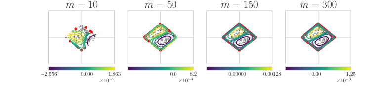
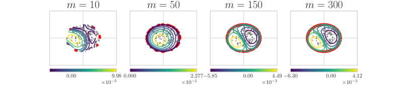
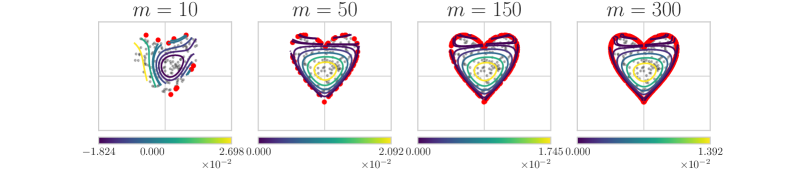
Figure 3: Contour lines of the optimal $\tilde{g}_{0}$ (first dimension of $\tilde{\boldsymbol{g}}$) output by TKSD across different values of $m$ and differently shaped truncation boundaries: the $\ell_{1}$ ball (top), the $\ell_{2}$ ball (middle) and a heart shape (bottom). Red points are all $m$ points in $\widetilde{\partial V}$ and grey points are samples from the truncated dataset. Note that we plot only the first dimension of $\tilde{\boldsymbol{g}}$ (i.e. $g_{1}$), but we observe the same pattern with the second dimension.

B.2 Comparison between increasing $n_{\varepsilon_{m}}$ and $m$ in Remark 5.4

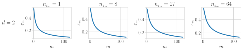
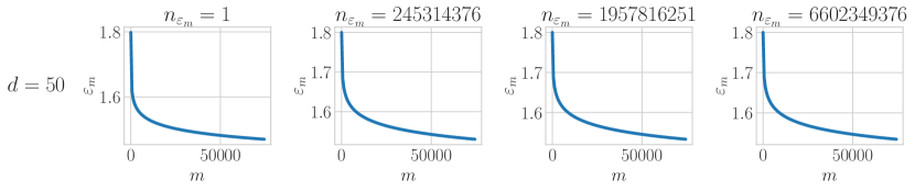
Figure 4: Upper bound on $\varepsilon_{m}$ (given in (19)) against $m$, the number of finite boundary points, plotted for different values of fixed dimension $d$ and $n_{\varepsilon_{m}}$, which scales cubically.

In Figure 4 we show that $\varepsilon_{m}$, as defined in Proposition 5.3, is a decreasing function of $m$, no matter how large $n_{\varepsilon_{m}}$ becomes. In this example, $n_{\varepsilon_{m}}$ is scaling cubically, whereas $m$ is scaling linearly. Across all values of $n_{\varepsilon_{m}}$, $\varepsilon_{m}$ is decreasing fast with respect to $m$. This empirically justifies the statement given in Remark 5.4.

B.3 Empirical Consistency

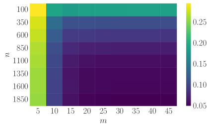
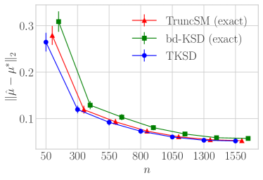
Figure 5: Left: Estimation error as $n$ and $m$ increases for TKSD only. Right: Mean estimation error for the three methods: TKSD, TruncSM and bd-KSD, with standard error bars. TKSD uses a fixed $m=32$ across all values of $n$. Both plots report statistics over 64 seeds.

We verify that (26) is consistent estimator via empirical experiments. Note that for consistency as proven in Theorem 5.10, we require taking the limit as $m\to\infty$, after which the estimator is consistent for $n$. So as $m$ and $n$ increases, the estimation error decreases towards zero. We show consistency as $m$ and $n$ increase empirically in Figure 5, for a simple experiment setup, similar to the setup from Section 6.3. Data are simulated from $\mathcal{N}(\boldsymbol{\mu}^{\star},I_{d})$, where $d=2$, $\boldsymbol{\mu}^{\star}=[0.5,0.5]^{\top}$, and $I_{d}$ is known. Data are truncated to the $\ell_{2}$ ball until we reach $n$ many data points (after truncation).

The aim of estimation is $\boldsymbol{\mu}^{\star}$. Across 64 trials, Figure 5 shows plots of the mean estimation error, given by $\|\boldsymbol{\hat{\mu}}-\boldsymbol{\mu}^{\star}\|$, where $\boldsymbol{\hat{\mu}}$ is the corresponding estimate of $\boldsymbol{\mu}^{\star}$ output by a given method. In the first plot (left), we show that as both $n$ and $m$ increase, the estimation error for TKSD decreases towards zero. In the second plot (right), for a fixed $m$, we show that the rate of convergence as $n$ increases for TKSD matches that of bd-KSD and TruncSM.

B.4 Gaussian Mixture Experiment

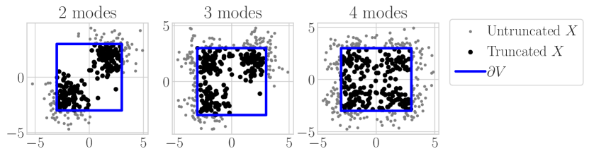
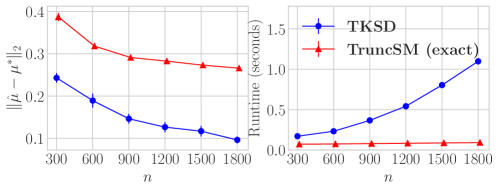
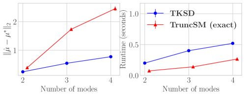
Figure 6: Top: example setup for the experiment as the number of mixture modes increases from 2 to 4. Middle: estimation error as $n$ increases for 2 mixture modes, averaged across 256 seeds. Bottom: Estimation error as the number of mixture modes increases for a fixed $n=300$, averaged across 256 seeds.

As an additional experiment to show the capability of the method, we test on a more complex problem, estimating several means of a Gaussian Mixture distribution. The estimation task is as follows. Fix $d=2$ and $m=200$. Let the mixture modes be given as follows,

$$\boldsymbol{\mu}_{1}^{*}=[1.5,1.5]^{\top},\;\boldsymbol{\mu}_{2}^{*}=[-1.5,-1.5]^{\top},\;\boldsymbol{\mu}_{3}^{*}=[-1.5,1.5]^{\top},\;\boldsymbol{\mu}_{4}^{*}=[1.5,-1.5]^{\top}.$$

We independently simulate samples from $\mathcal{N}(\boldsymbol{\mu}_{i}^{*},I_{d})$, for $i=1,\dots,4$, and truncate these samples to within a box with vertices at $[-3,-3]$, $[3,-3]$, $[-3,3]$ and $[3,3]$ until we reach a total of $n$ samples after truncation. Figure 6, top, shows an example of this experiment setup.

The task is to estimate $\boldsymbol{\mu}^{*}_{i}$ for all $i$. To ensure a well specified experiment, we set the initial conditions as a perturbation from the true value, i.e. $\boldsymbol{\mu}_{i}^{\text{ini}}=\boldsymbol{\mu}^{*}_{i}+\boldsymbol{z}$, $\boldsymbol{z}\sim\mathcal{N}(\boldsymbol{0},0.5\cdot I_{2})$. We estimate $\boldsymbol{\mu}$ with TKSD and compare it to a corresponding estimate by TruncSM across a range of different values of $n$ and number of mixture modes, shown in Figure 6, middle and bottom. Overall, TKSD significantly outperforms TruncSM in this experiment across all variations at the cost of runtime.

B.5 Regression

We provide a further example of using TKSD to estimate the parameters of a regression problem. First, we simulate data in the following way:

$$y_{i}\sim\mathcal{N}(\mu_{i},1),\;\mu_{i}=\beta_{0}+\beta_{1}x_{i},\;x_{i}\sim\mathrm{Uniform}(0,1)$$

where we know the true values, $\beta_{0}^{\star}=3$ and $\beta_{1}^{\star}=4$. We truncate the dataset to where $y_{i}\geq 5\;\forall i$, so only a portion of both $y$ and $x$ are observed. We then estimate the conditional density $p(y|x)$ by minimising the TKSD divergence to estimate $\beta_{0}$ and $\beta_{1}$.

We obtain the log-likelihood of the Normal distribution under the estimates of $\beta_{0}$ and $\beta_{1}$ given by TKSD. Additionally, we also measure the log-likelihood of a truncated Normal distribution, which is tractable for $d=1$, using the same estimates. We compare these log-likelihoods to ones obtained by a naive MLE approach which does not account for truncation. As an additional measure, we calculate the non-truncated test error, which is the mean squared error between the non-truncated and hence unobserved values of $y$ (i.e. the data points that were truncated in the data simulation process, where $y_{i}<5\;\forall i$) and their corresponding predictions. A histogram of these log-likelihoods and test errors is given in the left panel of Figure 7, and an example of one such simulated regression is given in the top-right. Overall, the log-likelihoods obtained by TKSD are significantly higher than MLE, and the test errors are significantly smaller, showing the improvement of TKSD over the naive approach.

We also experiment on a real-world dataset given by UCLA: Statistical Consulting Group (Example 1). This dataset contains student test scores in a school for which the acceptance threshold is 40 out of 100, and therefore the response variable (the test scores) are truncated below by 40 and above by 100. Since no scores get close to 100, we only consider one-sided truncation at $y=40$. The aim of the regression is to model the response variable, the test scores, based on a single covariate of each students’ corresponding score on a different test. The bottom-right panel of Figure 7 shows the plotted dataset and the regression line fit by TKSD and naive MLE. Whilst we have no true baseline value to compare to, the TKSD regression line seems to account for the truncation, whilst as expected, MLE does not.

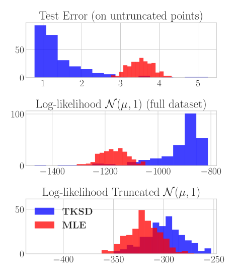
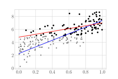
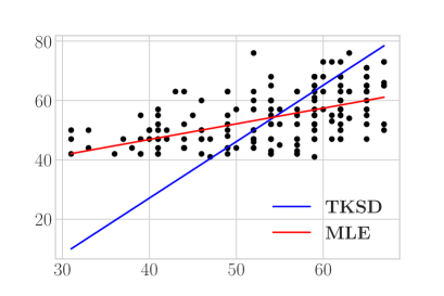
Figure 7: Statistics from regression fit. Left: Test error calculated only on non-truncated points (top), log-likelihood over full dataset for a $\mathcal{N}(\mu,1)$ distribution (middle) and the log-likehood over a truncated Normal distribution with mean $\mu$ and variance 1 (bottom). Right: Example of TKSD used to fit two regression tasks; simulated data (top) and a real dataset (bottom). Fuller black points are the observed data points, after truncation, and smaller grey points are the unobserved data points that were truncated out in the data simulation process.

B.6 Quantifying Effect of Boundary Point Distribution

We test whether the effect of boundary point sampling distribution has an effect on the robustness of TKSD. To do so, we repeat the simple experiment setup where data are simulated as follows,

$$\boldsymbol{x}\sim\mathcal{N}(\boldsymbol{\mu}^{\star},\boldsymbol{I}_{2}),\;\boldsymbol{\mu}^{\star}=\begin{bmatrix}1,&1\end{bmatrix}^{\top}$$

from which we observe $n=400$ realisations of $\boldsymbol{x}$ that are restricted to the unit $\ell_{2}$ ball around the origin, and let $m=30$. We use TKSD to provide an estimate $\boldsymbol{\hat{\mu}}$ of $\boldsymbol{\mu}^{\star}$ under three scenarios:

1. Boundary points are distributed towards $\boldsymbol{\mu}^{\star}$, i.e. samples from $\widetilde{\partial V}$ are closer to the centre of the dataset.

2. Boundary points are distributed away from $\boldsymbol{\mu}^{\star}$, i.e. samples from $\widetilde{\partial V}$ are closer to the edge of the dataset.

3. Boundary points are sampled uniformly across $\partial V$.

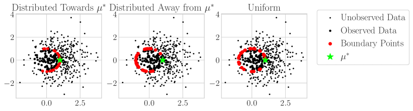
Figure 8: Example of experiment setup for measuring the effect of the boundary point distribution.

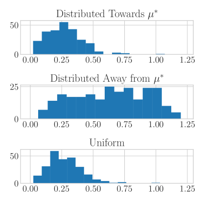
Figure 9: Frequency of estimation errors ($\|\boldsymbol{\hat{\mu}}-\boldsymbol{\mu}^{\star}\|$) in the simple experiment setup for the three differently distributed boundary points.

See Figure 8 for a visual representation of these three scenarios. We measure the estimation error, $\|\boldsymbol{\hat{\mu}}-\boldsymbol{\mu}^{\star}\|$, and test whether one scenario provides a lower error on average overall. Figure 9 shows the distribution of all three estimation errors across 256 trials. Scenario 1 and 3 provide comparable error distributions which are significantly smaller than the error distribution of scenario 2, implying that either the boundary needs to be covered fully, or the boundary points need to be ‘representative’ in some way, where the most significant truncation effect is.

B.7 Choosing Boundary Size for Dimension Benchmarks

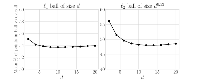
Figure 10: Mean percentage of points which remain after truncation as dimension $d$ increases, where the truncation domain is a $\ell_{c}$ ball of radius $d$ for $c=1$ (left), and $d^{0.53}$ for $c=2$ (right).

In Section 6.3, we chose the size of the boundary to scale with $d$ so that roughly the same amount of data points are truncated for each value of dimension $d$. The values of $d$ and $d^{0.53}$ for the $\ell_{1}$ ball and $\ell_{2}$ ball respectively were chosen via trial and error such that the percentage of points simulated from the Normal distribution remaining after truncation did not vary significantly. Figure 10 shows that with this choice of $\ell_{1}$ and $\ell_{2}$ ball radius, the mean percentage of points that remain after truncation remains at roughly 50% in both cases.

B.8 Extra Computation Details

• The inversion of $\mathbf{K}^{\prime}$ is the largest computational expense when it comes to evaluating the $U$-statistic or $V$-statistic ((24) and (25) respectively).

  If $m<d$, which will be common as we want $m$ to be large, then $\mathbf{K}^{\prime}$ is rank deficient. To circumvent this issue, we invert $\mathbf{K}^{\prime}+\epsilon\mathbf{I}_{m}$ instead, where $\epsilon>0$ is small. Additionally, $\mathbf{K}^{\prime}+\epsilon\mathbf{I}_{m}$ is symmetric and positive definite, so we can exploit its Cholesky decomposition to make the inversion faster and more stable.

  Overall, this inversion looks like

  $$(\mathbf{K}^{\prime})^{-1}\approx(\mathbf{K}^{\prime}+\epsilon\mathbf{I}_{m})^{-1}=\mathbf{L}^{-1}(\mathbf{L}^{-1})^{\top},$$

  where $\mathbf{L}$ is the corresponding lower triangular matrix from the Cholesky decomposition of $\mathbf{K}^{\prime}+\epsilon\mathbf{I}_{m}$. The inversion of $\mathbf{L}$, a lower triangular matrix, requires half as many operations as inverting $\mathbf{K}+\epsilon\mathbf{I}_{m}$ directly (Krishnamoorthy & Menon, 2013).

• We also make use of methods presented in Jitkrittum et al. (2017) for fast computation when constructing all kernel matrices in Python.

References

- Barp et al. (2019) Barp, A., Briol, F.-X., Duncan, A., Girolami, M., and Mackey, L. Minimum stein discrepancy estimators. In Advances in Neural Information Processing Systems, volume 32, 2019.
- Boyd & Vandenberghe (2004) Boyd, S. and Vandenberghe, L. Convex optimization. Cambridge university press, 2004.
- Chen et al. (2011) Chen, L. H., Goldstein, L., and Shao, Q.-M. Normal approximation by Stein’s method, volume 2. Springer, 2011.
- Chwialkowski et al. (2016) Chwialkowski, K., Strathmann, H., and Gretton, A. A kernel test of goodness of fit. In Proceedings of The 33rd International Conference on Machine Learning, volume 48 of Proceedings of Machine Learning Research, pp. 2606–2615. PMLR, 2016.
- Gorham & Mackey (2015) Gorham, J. and Mackey, L. Measuring sample quality with stein's method. In Advances in Neural Information Processing Systems, volume 28. Curran Associates, Inc., 2015.
- Gorham et al. (2020) Gorham, J., Raj, A., and Mackey, L. Stochastic stein discrepancies. In Advances in Neural Information Processing Systems, volume 33, pp. 17931–17942. Curran Associates, Inc., 2020.
- Gutmann & Hyvärinen (2010) Gutmann, M. and Hyvärinen, A. Noise-contrastive estimation: A new estimation principle for unnormalized statistical models. In Proceedings of the 13th International Conference on Artificial Intelligence and Statistics, volume 9 of Proceedings of Machine Learning Research, pp. 297–304. PMLR, 2010.
- Gutmann & Hyvärinen (2012) Gutmann, M. U. and Hyvärinen, A. Noise-contrastive estimation of unnormalized statistical models, with applications to natural image statistics. Journal of Machine Learning Research, 13(11):307–361, 2012.
- Hyvärinen (2005) Hyvärinen, A. Estimation of non-normalized statistical models by score matching. Journal of Machine Learning Research, 6(24):695–709, 2005.
- Hyvärinen (2007) Hyvärinen, A. Some extensions of score matching. Computational statistics & data analysis, 51(5):2499–2512, 2007.
- Jitkrittum et al. (2017) Jitkrittum, W., Xu, W., Szabo, Z., Fukumizu, K., and Gretton, A. A linear-time kernel goodness-of-fit test. In Advances in Neural Information Processing Systems, volume 30. Curran Associates, Inc., 2017.
- Kalos & Whitlock (2009) Kalos, M. H. and Whitlock, P. A. Monte carlo methods. John Wiley & Sons, 2009.
- Kanagawa et al. (2019) Kanagawa, H., Jitkrittum, W., Mackey, L., Fukumizu, K., and Gretton, A. A kernel stein test for comparing latent variable models. arXiv preprint arXiv:1907.00586, 2019.
- Krishnamoorthy & Menon (2013) Krishnamoorthy, A. and Menon, D. Matrix inversion using cholesky decomposition. In 2013 signal processing: Algorithms, architectures, arrangements, and applications (SPA), pp. 70–72. IEEE, 2013.
- Lin et al. (2016) Lin, L., Drton, M., and Shojaie, A. Estimation of high-dimensional graphical models using regularized score matching. Electronic journal of statistics, 10(1):806, 2016.
- Liu et al. (2016) Liu, Q., Lee, J., and Jordan, M. A kernelized stein discrepancy for goodness-of-fit tests. In Proceedings of The 33rd International Conference on Machine Learning, volume 48 of Proceedings of Machine Learning Research, pp. 276–284. PMLR, 2016.
- Liu et al. (2022) Liu, S., Kanamori, T., and Williams, D. J. Estimating density models with truncation boundaries using score matching. Journal of Machine Learning Research, 23(186):1–38, 2022.
- Pang et al. (2020) Pang, T., Xu, K., Li, C., Song, Y., Ermon, S., and Zhu, J. Efficient learning of generative models via finite-difference score matching. In Advances in Neural Information Processing Systems, volume 33, pp. 19175–19188, 2020.
- Serfling (2009) Serfling, R. J. Approximation theorems of mathematical statistics. John Wiley & Sons, 2009.
- Sharrock et al. (2022) Sharrock, L., Simons, J., Liu, S., and Beaumont, M. Sequential neural score estimation: Likelihood-free inference with conditional score based diffusion models. arXiv preprint arXiv:2210.04872, 2022.
- Shi et al. (2021) Shi, J., Liu, C., and Mackey, L. Sampling with mirrored stein operators. arXiv preprint arXiv:2106.12506, 2021.
- Song & Ermon (2019) Song, Y. and Ermon, S. Generative modeling by estimating gradients of the data distribution. In Advances in Neural Information Processing Systems, volume 32, 2019.
- Song & Kingma (2021) Song, Y. and Kingma, D. P. How to train your energy-based models. arXiv preprint arXiv:2101.03288, 2021.
- Song et al. (2021) Song, Y., Sohl-Dickstein, J., Kingma, D. P., Kumar, A., Ermon, S., and Poole, B. Score-based generative modeling through stochastic differential equations. In International Conference on Learning Representations, 2021.
- Stein (1972) Stein, C. A bound for the error in the normal approximation to the distribution of a sum of dependent random variables. In Proceedings of the sixth Berkeley symposium on mathematical statistics and probability, volume 2: Probability theory, pp. 583–602. University of California Press, 1972.
- Steinwart & Christmann (2008) Steinwart, I. and Christmann, A. Support vector machines. Springer Science & Business Media, 2008.
- (27) UCLA: Statistical Consulting Group. Truncated regression — stata data analysis examples. URL https://stats.oarc.ucla.edu/stata/dae/truncated-regression/. Accessed March 17, 2023.
- Williams & Liu (2022) Williams, D. J. and Liu, S. Score matching for truncated density estimation on a manifold. In Topological, Algebraic and Geometric Learning Workshops 2022, pp. 312–321. PMLR, 2022.
- Wu et al. (2022) Wu, S., Diao, E., Elkhalil, K., Ding, J., and Tarokh, V. Score-based hypothesis testing for unnormalized models. IEEE Access, 10:71936–71950, 2022.
- Xu (2022) Xu, W. Standardisation-function kernel stein discrepancy: A unifying view on kernel stein discrepancy tests for goodness-of-fit. In International Conference on Artificial Intelligence and Statistics, pp. 1575–1597. PMLR, 2022.
- Xu & Matsuda (2021) Xu, W. and Matsuda, T. Interpretable stein goodness-of-fit tests on riemannian manifold. In Proceedings of the 38th International Conference on Machine Learning, volume 139 of Proceedings of Machine Learning Research, pp. 11502–11513. PMLR, 2021.
- Yang et al. (2018) Yang, J., Liu, Q., Rao, V., and Neville, J. Goodness-of-fit testing for discrete distributions via stein discrepancy. In Proceedings of the 35th International Conference on Machine Learning, volume 80 of Proceedings of Machine Learning Research, pp. 5561–5570. PMLR, 2018.
- Yu et al. (2016) Yu, M., Kolar, M., and Gupta, V. Statistical inference for pairwise graphical models using score matching. In Advances in Neural Information Processing Systems, volume 29, 2016.
- Yu et al. (2019) Yu, S., Drton, M., and Shojaie, A. Generalized score matching for non-negative data. Journal of Machine Learning Research, 20(76):1–70, 2019.
- Yu et al. (2021) Yu, S., Drton, M., and Shojaie, A. Generalized score matching for general domains. Information and Inference: A Journal of the IMA, 2021.