Curvature corrected tangent space-based approximation of manifold-valued data

Abstract

When generalizing schemes for real-valued data approximation or decomposition to data living in Riemannian manifolds, tangent space-based schemes are very attractive for the simple reason that these spaces are linear. An open challenge is to do this in such a way that the generalized scheme is applicable to general Riemannian manifolds, is global-geometry aware and is computationally feasible. Existing schemes have been unable to account for all three of these key factors at the same time.

In this work, we take a systematic approach to developing a framework that is able to account for all three factors. First, we will restrict ourselves to the – still general – class of symmetric Riemannian manifolds and show how curvature affects general manifold-valued tensor approximation schemes. Next, we show how the latter observations can be used in a general strategy for developing approximation schemes that are also global-geometry aware. Finally, having general applicability and global-geometry awareness taken into account we restrict ourselves once more in a case study on low-rank approximation. Here we show how computational feasibility can be achieved and propose the curvature-corrected truncated higher-order singular value decomposition (CC-tHOSVD), whose performance is subsequently tested in numerical experiments with both synthetic and real data living in symmetric Riemannian manifolds with both positive and negative curvature.

Keywords manifold-valued data  $\cdot$ manifold-valued tensors  $\cdot$ tensor approximation  $\cdot$ tensor decomposition  $\cdot$ Riemannian manifold  $\cdot$ symmetric Riemannian manifold  $\cdot$ tangent space linearization  $\cdot$ curvature correction  $\cdot$ dimension reduction  $\cdot$ low-rank approximation  $\cdot$ higher-order singular value decomposition

AMS subject classifications (MSC2020) 53Z50  $\cdot$ 15A69  $\cdot$ 90C26  $\cdot$ 90C30  $\cdot$ 53-04  $\cdot$ 53-08  $\cdot$ 49Q99

1 Introduction.

Manifold-valued data are becoming ubiquitous. By now classical applications from the imaging sciences include non-linear color spaces [20] such as the Chromaticity Brightness model ($\mathbb{S}^{2}\times\mathbb{R}$) and the Hue Saturation Value model ($\mathbb{S}^{1}\times\mathbb{R}^{2}$), InSAR imaging [59] ($\mathbb{S}^{1}$), Diffusion Tensor imaging [4] with the manifold of positive definite symmetric $3\times 3$ matrices ($\mathcal{P}(3)$) and Electron Backscatter Diffraction imaging [1] with the 3D rotation group ($\mathrm{SO}(3)$). Beyond the imaging sciences, the data sciences have popularized non-linear data embedding into Riemannian manifolds, as data in many domains have non-Euclidean features [12, 52]. That is, besides the Euclidean embedding [69] ($\mathbb{R}^{d}$) there has been a surge in work on spherical embeddings [56, 84] ($\mathbb{S}^{d}$), hyperbolic embeddings [49, 62, 75, 81] ($\mathbb{H}^{d}$), combinations of these through product manifold embedding [31, 71], and embedding into other non-constant curvature spaces such as the Grassmann manifold [42, 22] ($\mathrm{Gr}(d,k)$) and the space of symmetric positive definite matrices [79, 22] ($\mathcal{P}(d)$).

All of the above spaces are examples of symmetric Riemannian manifolds under their standard Riemannian metric. Arguably, there is a reason why symmetric spaces are very important to these communities. Indeed, the authors of [57] argue that symmetric spaces in the setting of data embeddings are a very natural, versatile and rich class of spaces for capturing the geometry of real-world data. For the imaging sciences, symmetric spaces are particularly useful from a more practical point of view, i.e., for constructing numerically efficient models [3, 6] and algorithms [9, 7, 26] through inexpensive evaluation of differentials or covariant derivatives of important mappings. The latter is possible due to a key property of symmetric spaces. That is, knowing the curvature at only one point yields a large amount of information about the global geometry of the space of interest.

Surprisingly, in downstream processing and analysing of manifold-valued data – e.g., dimension reduction for visualisation [33] or for retrieving underlying structure from (principal) sub-manifolds [27] – the symmetric structure is hardly ever used. Typically, works seem to choose between methods that are either global, but manifold-specific [34] or localized to a tangent space, but general [28]. Focusing on the latter class of approaches, subsequently quantifying the localization error is hardly ever addressed. Even for the seminal work on principal geodesic analysis (PGA) [27, 28] – which is in practice often implemented as a tangent space PCA – an approximation error analysis due to curvature effects is – to the best of our knowledge – still open for general (symmetric) Riemannian manifolds. Existing work that attempts to take curvature into account is still too local in nature [54], only covers specific manifolds [19, 67], or does not yield practical algorithms [73].

On the flip side, being able to use the full potential of symmetric Riemannian manifolds – in a curvature-aware tangent space-based framework – has two main advantages. First, it would enable one to open the doors for many more approximation methods beyond simple PCA, e.g., approaches based on classical decomposition schemes for matrices and tensors [51] and extensions to modern ones [14, 46, 45]. Secondly, and more practically, popular modern software packages for optimization and data analysis on manifolds [5, 60] are designed for the general setting so that one does not have to reinvent every method for new Riemannian manifolds. So motivated by the above, in this work we focus on the general problem of local, but curvature-aware approximation of the multi-dimensional manifold-valued array $\mathbfcal{X}\in\mathcal{M}^{d_{1}\times\cdots\times d_{n}}$ from some point $\mathbf{p}\in\mathcal{M}$ on a symmetric Riemannian manifold $\mathcal{M}$. That is, given a suitable class of approximators defined by a tangent space subset $\mathcal{S}_{\mathbf{p}}(\mathcal{M}^{d_{1}\times\ldots\times d_{n}})\subset\mathcal{T}_{\mathbf{p}}\mathcal{M}^{d_{1}\times\cdots\times d_{n}}$, we aim to construct a suitable approximation $\Xi_{\mathbf{p}}\in\mathcal{S}_{\mathbf{p}}(\mathcal{M}^{d_{1}\times\ldots\times d_{n}})$ such that the global approximation error,

$$d_{\mathcal{M}^{d_{1}\times\cdots\times d_{n}}}(\mathbfcal{X},\exp_{\mathbf{p}}(\Xi_{\mathbf{p}}))^{2},$$ (1)

is small, where $\exp_{\mathbf{p}}:\mathcal{T}_{\mathbf{p}}\mathcal{M}^{d_{1}\times\cdots\times d_{n}}\to\mathcal{M}^{d_{1}\times\cdots\times d_{n}}$ is the exponential mapping on the manifold $\mathcal{M}^{d_{1}\times\cdots\times d_{n}}$ and $d_{\mathcal{M}^{d_{1}\times\cdots\times d_{n}}}:\mathcal{M}^{d_{1}\times\cdots\times d_{n}}\times\mathcal{M}^{d_{1}\times\cdots\times d_{n}}\to\mathbb{R}$ is the distance. In particular, we aim for a generally applicable, numerically feasible and theoretically motivated approach to the approximation of the minimizer of eq. 1 that can be a framework for generalizing Euclidean schemes to Riemannian manifolds.

1.1 Related work.

Geometry of data has been considered in several forms. One worth mentioning is the setting of data in Euclidean space that lives on a lower-dimensional unknown manifold. Although this is strictly speaking a different setting than the problem stated in eq. 1 – where there is an explicit manifold and a specific notion of geometry –, algorithms developed for the implicit setting have to deal with similar challenges. In particular, there seems to be a trend that some notion of global geometry is necessary to build suitable algorithms. To give one example, but without going into detail, graph Laplacian-based approaches for low rank approximation [89, 90], non-negative matrix factorization [13, 32, 41] and low rank representation [70] are superior to naive methods that only consider the ambient Euclidean geometry.

In the case of an explicit manifold, there is more information available than in the above setting. This allows one to work in an intrinsic setting, where one can use several manifold mappings, rather than in an extrinsic one. It is less clear how the observations from the extrinsic case regarding necessity of global information should be translated to the intrinsic case. In the following we will briefly review developments in global and tangent space-based approaches to approximation of manifold-valued data. In particular, we will highlight several best practices and limitations and argue where there are missed opportunities. The following overview will mainly focus on the order 1 case, i.e., when the manifold-valued data lives in $\mathcal{M}^{d_{1}}$ for some $d_{1}\in\mathbb{N}$. This is for the simple reason that to the best of our knowledge there is no existing work on tensor-decomposition approaches for manifold-valued data in the spirit of [51].

Global approaches to approximation.

In the intrinsic setting, it seems natural – as Riemannian manifolds do not have a well-defined notion of an origin – to design methods globally. For the decomposition of data into nested geodesic subspaces, numerically efficient schemes for several manifolds have been proposed in a global fashion. In particular, for nested geodesic subspaces of spheres and hyperbolic spaces [76] or on polyspheres and Grassmann manifolds [23], the manifold-specific Riemannian structure gives practical algorithms. If the constraint of having geodesic subspaces is relaxed, there is the famous nested spheres framework [47] and the recent generalisation to Grassmann manifolds [85].

Even though the above methods perform very well for their respective manifolds, it is hard to adapt these methods to a general setting. There have been attempts to generalize nested (non-)geodesic subspace frameworks, but these run into practical challenges. One issue is that even when a method is general, implementation relies on a manifold-specific mapping [58]. More common is the issue that the proposed method has a hard time scaling up. In particular, it can be hard to scale up to high-dimensional manifolds due to non-convexity of the proposed subspace construction problem [24, 64], or to scale up to multidimensional subspaces either due to construction restrictions [37, 63] or due to curse of dimensionality [72, 86].

Besides the approximation approaches outlined in the above, which are all similar in spirit to doing a low rank approximation, there have been methods trying to generalize other approximation schemes. All of these come with their own challenges in terms of generalizability, but nevertheless work well for their respective manifolds. In particular, low rank representation for the Grassmann manifold as proposed in [83] and [65] relies on linearity even though the manifold is a quotient space, which renders the definition ambiguous and hard to generalize. Similarly, in [82] low-rank representation is proposed for the space of symmetric positive definite matrices, where again the ambient linearity is used. Although using linearity is less of an issue for the latter approach, the definition depends on a specific metric, once more making generalization challenging. Another example of a numerically successful, but hard to generalize method is [35], in which a kernel approach is used to generalize dictionary learning on the space of symmetric positive definite matrices. Here the design of the kernel – reflecting the global geometry of the space – is heavily dependent on the Riemannian manifold structure of this matrix manifold.

Finally, we would like to point out that there are exceptions to this recurring issue of global methods being unable to generalize. For example, basic multiscale methods such as [66] do well in terms of general applicability and computational feasibility. However, adding more structure to such a scheme may arguably be challenging. Indeed, the authors of [30] point out that adding extra structure such as bi-orthogonal wavelet structure comes with definability issues.

Tangent space approaches to approximation.

Perhaps unsurprisingly after the above discussion, tangent space-based methods are very popular due to their general applicability with respect to the underlying manifold. Besides their generality from a geometric point of view, the tangent space setting is more often than not the only framework in which it is even possible to generalize approximation and decomposition schemes from the Euclidean case to the general Riemannian manifold setting. Indeed, even though low rank-like approaches make sense for both global versions – as discussed above – and tangent space versions – e.g., the aforementioned PGA framework [27, 28] –, other methods such as dictionary learning [29, 40, 87] can only be defined in the tangent space. In other words, there is a case to make for the idea of generalizing Euclidean approaches to the tangent space setting.

There are two main challenges that come with a tangent space-based approach: where to linearize and how to take the global structure of the manifold into account in a computationally feasible way. Regarding the former challenge, it should be mentioned that one has to be careful when choosing a point of linearization as argued by the authors of [44] in the case of spheres and later for shape space [43]. However, these are issues one can deal with by being careful or passing to a framework where the point of linearization is also optimized over [88]. Arguably, the key open problem for basically any tangent space-based method is the latter challenge, i.e., a principled way to capture global geometry without sacrificing computational feasibility. To be more concrete, even though it is occasionally possible to take global structure into account, computational feasibility tends to suffer from subsequent adaptations. Once more, a prime example is the seminal work [27, 28] by Fletcher et al. on PGA. In particular, although the original method was proposed in an exact form that took global geometry into account, linearization allowed for actually computing it cheaply. Later work on solving the exact version in a general setting [73] or for specific manifolds [19, 54, 67] yielded slow algorithms without any convergence guarantees due to non-convexity of this geometry-aware subspace construction problem.

1.2 Specific contributions.

The contributions in this article are the theory and algorithm development for computationally feasible and geometry-aware tangent space-based methods for approximating manifold-valued data living in symmetric Riemannian manifolds.

First, we would like to point out that this article is, to the best of our knowledge, the first work to address approximation of multidimensional manifold-valued arrays in a tensor decomposition setting. Furthermore, this article is, to the best of our knowledge, the first to give a provably complete account of the most important effects of the global geometry on naive tangent space-based approximation schemes on symmetric Riemannian manifolds and to propose a general way of correcting for these effects. Finally, we showcase how the developed theory can be used to construct a numerically feasible and geometry-aware low (multi-linear) rank approximation scheme for general symmetric Riemannian manifolds. More specifically, the contributions are the following.

Quantifying the role of curvature on symmetric Riemannian manifolds.

We analyze the global approximation error eq. 1 on Riemannian manifolds and show that for symmetric Riemannian manifolds the leading term is fully determined by the tangent space approximation error and the curvature at the point of linearization, which is our main theoretical result. In particular, we find that, if not corrected for, negative curvature can amplify seemingly minor errors exponentially, whereas seemingly large errors on a positively curved space can be diminished.

Curvature corrected approximation of manifold-valued tensors.

Based on the analysis, we propose a curvature corrected approximation error. In addition, we show that under mild conditions, minimizing the proposed error will decrease the discrepancy to the original approximation error eq. 1. In other words, minimizing the curvature corrected approximation error will yield a low original approximation error. Moreover, we will show that the curvature corrected approximation error has several nice properties such as a lower bound on the approximation error and stability with respect to vanishing curvature effects.

Efficient and curvature corrected low multi-linear rank approximation.

In a case study on low multi-linear rank approximation, we will use the developed theory and propose curvature corrected truncated higher-order singular value decomposition (CC-tHOSVD), which boils down to a truncated higher-order singular value decomposition and a curvature correction step that consists of solving a linear system of equations. We test the proposed method on synthetic 1D and real 2D manifold-valued data and on positive and negative-curvature manifolds to showcase that this method indeed overcomes the long-standing open problems of being generally applicable to different manifolds, taking global geometry into account properly and being numerically feasible.

1.3 Outline.

This article is structured as follows. Section 2 covers several notation conventions that will help the reader to keep the various objects apart throughout the rest of the work, and introduces manifold-valued tensors, the main object of interest in this article, along with several related notions. In sections 3, 4 and 5 the core theoretical ideas for realizing generally applicable, global-geometry aware and computationally feasible manifold-valued tensor approximation are developed. In particular, in section 3 we state and prove our main theoretical result (theorem 3.4), which states that on general symmetric Riemannian manifolds, the leading order term in the global approximation error eq. 1 is fully determined by the tangent space approximation error and and the curvature at the point of linearization. In section 4 we will show that the general result from section 3 can be used to realize global-geometry aware manifold-valued tensor approximation. Next, in a case study on low multi-linear rank approximation in section 5, we argue that computational feasibility can also be attained, which will be tested thoroughly through several numerical experiments in section 6. Finally, we summarize our findings in section 7.

2 Notation.

2.1 Differential and Riemannian geometry.

Here we present some basics and notation from differential and Riemannian geometry, see [10, 15, 55, 68] for more details.

Let $\mathcal{M}$ be a smooth manifold. We write $C^{\infty}(\mathcal{M})$ for the space of smooth functions over $\mathcal{M}$. The tangent space at $\mathbf{p}\in\mathcal{M}$ – defined as the space of all derivations at $\mathbf{p}$ – is denoted by $\mathcal{T}_{\mathbf{p}}\mathcal{M}$ and for tangent vectors we write $\Xi_{\mathbf{p}}$. For the tangent bundle we write $\mathcal{T}\mathcal{M}$ and vector fields – defined as sections of the tangent bundle – are written as $\mathscr{X}(\mathcal{M})\subset\mathcal{T}\mathcal{M}$. Furthermore, additional structure and on manifolds and derived notions thereof are typically defined through tensor fields of the form $T~{}:~{}\mathscr{X}(\mathcal{M})^{n}\to\mathscr{X}(\mathcal{M})^{m}$ or $T~{}:~{}\mathscr{X}(\mathcal{M})^{n}\to C^{\infty}(\mathcal{M})$. A tensor field can – by definition of being $C^{\infty}(\mathcal{M})$-modules – be restricted to a tangent space at each point $\mathbf{p}\in\mathcal{M}$, for which we use the notation $T_{\mathbf{p}}:\mathcal{T}_{\mathbf{p}}\mathcal{M}^{n}\to\mathcal{T}_{\mathbf{p}}\mathcal{M}^{m}$ or $T_{\mathbf{p}}:\mathcal{T}_{\mathbf{p}}\mathcal{M}^{n}\to\mathbb{R}$.

A smooth manifold $\mathcal{M}$ becomes a Riemannian manifold if it is equipped with a smoothly varying metric tensor field $(\,\cdot\,,\,\cdot\,)\colon\mathscr{X}(\mathcal{M})\times\mathscr{X}(\mathcal{M})\to C^{\infty}(\mathcal{M})$. This tensor field induces a (Riemannian) metric $d_{\mathcal{M}}\colon\mathcal{M}\times\mathcal{M}\to\mathbb{R}_{\geq 0}$. The metric tensor can also be used to construct a unique affine connection, the Levi-Civita connection that is denoted by $\nabla_{(\,\cdot\,)}(\,\cdot\,):\mathscr{X}(\mathcal{M})\times\mathscr{X}(\mathcal{M})\to\mathscr{X}(\mathcal{M})$. This connection is in turn the cornerstone of a myriad of manifold mappings. One is the notion of a geodesic, which for two points $\mathbf{p},\mathbf{q}\in\mathcal{M}$ is defined as a curve $\gamma_{\mathbf{p},\mathbf{q}}\colon[0,1]\to\mathcal{M}$ with minimal length that connects $\mathbf{p}$ with $\mathbf{q}$. This notion is well-defined if the manifold is geodesically connected, i.e., any two points $\mathbf{p},\mathbf{q}\in\mathcal{M}$ can be connected with a geodesic that is contained in $\mathcal{M}$. Another closely related notion is the curve $t\mapsto\gamma_{\mathbf{p},\Xi_{\mathbf{p}}}(t)$ for a geodesic starting from $\mathbf{p}\in\mathcal{M}$ with velocity $\dot{\gamma}_{\mathbf{p},\Xi_{\mathbf{p}}}(0)=\Xi_{\mathbf{p}}\in\mathcal{T}_{\mathbf{p}}\mathcal{M}$. This can be used to define the exponential map $\exp_{\mathbf{p}}\colon\mathcal{G}_{\mathbf{p}}\to\mathcal{M}$ as

$$\exp_{\mathbf{p}}(\Xi_{\mathbf{p}}):=\gamma_{\mathbf{p},\Xi_{\mathbf{p}}}(1)\quad\text{where $\mathcal{G}_{\mathbf{p}}\subset\mathcal{T}_{\mathbf{p}}\mathcal{M}$ is the set on which $\gamma_{\mathbf{p},\Xi_{\mathbf{p}}}(1)$ is defined.}$$

The manifold $\mathcal{M}$ is said to be complete whenever $\mathcal{G}_{p}=\mathcal{T}_{\mathbf{p}}\mathcal{M}$. Furthermore, the logarithmic map $\log_{\mathbf{p}}\colon\exp(\mathcal{G}^{\prime}_{\mathbf{p}})\to\mathcal{G}^{\prime}_{\mathbf{p}}$ is defined as the inverse of $\exp_{\mathbf{p}}$, so it is well-defined on $\mathcal{G}^{\prime}_{\mathbf{p}}\subset\mathcal{G}_{\mathbf{p}}$ where $\exp_{\mathbf{p}}$ is a diffeomorphism. Finally, we write $R(\,\cdot\,,\,\cdot\,)(\,\cdot\,)\colon\mathscr{X}(\mathcal{M})\times\mathscr{X}(\mathcal{M})\times\mathscr{X}(\mathcal{M})\to\mathscr{X}(\mathcal{M})$ for the curvature tensor field, which can be used to define the sectional curvature $K_{\mathbf{p}}:\mathcal{T}_{\mathbf{p}}\mathcal{M}\times\mathcal{T}_{\mathbf{p}}\mathcal{M}\to\mathbb{R}$ at a point $\mathbf{p}\in\mathcal{M}$ as

$$K_{\mathbf{p}}(\Xi_{\mathbf{p}},\Theta_{\mathbf{p}}):=\left\{\begin{matrix}\frac{(R_{\mathbf{p}}(\Xi_{\mathbf{p}},\Theta_{\mathbf{p}})\Theta_{\mathbf{p}},\Xi_{\mathbf{p}})_{\mathbf{p}}}{\|\Xi_{\mathbf{p}}\|_{\mathbf{p}}^{2}\|\Theta_{\mathbf{p}}\|_{\mathbf{p}}^{2}-(\Xi_{\mathbf{p}},\Theta_{\mathbf{p}})_{\mathbf{p}}^{2}}&\text{if $\Xi_{\mathbf{p}},\Theta_{\mathbf{p}}\in\mathcal{T}_{\mathbf{p}}\mathcal{M}$ are linearly independent},\\ 0&\text{otherwise}.\\ \end{matrix}\right.$$

2.2 Manifold-valued tensors.

In the following we will be concerned with multi-dimensional manifold-valued arrays. To stay close to the vocabulary from the decomposition of multi-dimensional real-valued arrays, i.e., the field of tensor decompositions, we will use the following definition.

Definition 2.1 (manifold-valued tensors).

The space of manifold-valued tensors of order $n$ and size $d_{1}\times\cdots\times d_{n}$ is denoted as the Riemannian manifold $\mathcal{M}^{d_{1}\times\cdots\times d_{n}}$ equipped with the standard product metric. The elements of a tensor $\mathbfcal{X}\in\mathcal{M}^{d_{1}\times\cdots\times d_{n}}$ are denoted by $\mathbfcal{X}_{i_{1},\cdots,i_{n}}$.

The notion of a manifold-valued tensor or real-valued tensor is not to be confused with the notion of a tensor field in the setting of differential geometry. In this work, the only tensor fields will be the metric tensor field and the curvature tensor field, both of which have special names and were introduced with special notation in section 2.1. To avoid any further confusion we will always talk about manifold-valued tensors and real-valued tensors and use an appropriate notation convention as well. In particular, manifold-valued tensors, real-valued tensors, real-valued matrices and vectors, points on a manifold, and scalars are denoted in different typeface for clarity. Throughout this paper, calligraphic and boldface capital letters are used for manifold-valued or real-valued tensors, boldface capital letters are used for real-valued matrices, lower boldface letters for real-valued vectors or points on a manifold, and regular letters for scalars.

Distance and norm.

Because $\mathbfcal{X}\in\mathcal{M}^{d_{1}\times\cdots\times d_{n}}$ does not live in a linear space, we do not have a manifold-valued tensor norm directly, but we do have a distance, which we inherit from the product manifold-structure

$$d_{\mathcal{M}^{d_{1}\times\cdots\times d_{n}}}(\mathbfcal{X},\mathbfcal{Y}):=\sqrt{\sum_{i_{1},\ldots,i_{n}=1}^{d_{1},\cdots,d_{n}}d_{\mathcal{M}}(\mathbfcal{X}_{i_{1},\ldots,i_{n}},\mathbfcal{Y}_{i_{1},\ldots,i_{n}})^{2}},\quad\mathbfcal{X},\mathbfcal{Y}\in\mathcal{M}^{d_{1}\times\cdots\times d_{n}}.$$ (2)

Furthermore, as mentioned in section 1 we will develop all of the analysis in a chosen tangent space $(\mathcal{T}_{\mathbf{p}}\mathcal{M})^{d_{1}\times\cdots\times d_{n}}$ for $\mathbf{p}\in\mathcal{M}$. For notational convenience we will write $\mathcal{T}_{\mathbf{p}}\mathcal{M}^{d_{1}\times\cdots\times d_{n}}$ for the tangent space and for tangent vectors we write $\Xi_{\mathbf{p}}\in\mathcal{T}_{\mathbf{p}}\mathcal{M}^{d_{1}\times\cdots\times d_{n}}$. The tangent space $\mathcal{T}_{\mathbf{p}}\mathcal{M}^{d_{1}\times\cdots\times d_{n}}$ is normed through the product metric tensor, i.e., the norm of a tangent vector $\Xi_{\mathbf{p}}\in\mathcal{T}_{\mathbf{p}}\mathcal{M}^{d_{1}\times\cdots\times d_{n}}$ is given by

$$\|\Xi_{\mathbf{p}}\|_{\mathbf{p}}:=\Bigl{(}\sum_{i_{1},\ldots,i_{n}}^{d_{1},\ldots,d_{n}}\|(\Xi_{\mathbf{p}})_{i_{1},\ldots,i_{n}}\|_{\mathbf{p}}^{2}\Bigr{)}^{\frac{1}{2}}$$ (3)

Pointwise manifold mappings.

The norm in eq. 3 is in some sense defined pointwise in $\mathbf{p}$. In the following we will often use several manifold mappings in a similar fashion. That is, we write for geodesics

$$\gamma_{\mathbf{p},\mathbfcal{X}}(t):=\bigl{(}\gamma_{\mathbf{p},\mathbfcal{X}_{i_{1},\ldots,i_{n}}}(t)\bigr{)}_{i_{1},\ldots,i_{n}=1}^{d_{1},\cdots,d_{n}}.$$ (4)

Similarly, for the exponential and logarithmic mappings we write

$$\exp_{\mathbf{p}}(\Xi_{\mathbf{p}}):=\bigl{(}\exp_{\mathbf{p}}((\Xi_{\mathbf{p}})_{i_{1},\ldots,i_{n}})\bigr{)}_{i_{1},\ldots,i_{n}=1}^{d_{1},\cdots,d_{n}},\quad\text{and}\quad\log_{\mathbf{p}}\mathbfcal{X}:=\bigl{(}\log_{\mathbf{p}}\mathbfcal{X}_{i_{1},\ldots,i_{n}}\bigr{)}_{i_{1},\ldots,i_{n}=1}^{d_{1},\cdots,d_{n}}$$ (5)

and for the distance we write

$$d_{\mathcal{M}^{d_{1}\times\cdots\times d_{n}}}(\mathbf{p},\mathbfcal{X}):=\sqrt{\sum_{i_{1},\ldots,i_{n}=1}^{d_{1},\cdots,d_{n}}d_{\mathcal{M}}(\mathbf{p},\mathbfcal{X}_{i_{1},\ldots,i_{n}})^{2}}.$$ (6)

Mode-$k$ unfolding.

An $n$ mode manifold-valued tensor $\mathbfcal{X}$ can be reshaped into a manifold-valued tensor array – i.e., a manifold-valued tensor of order $1$ consisting of manifold-valued tensors of order $n-1$ –, in $n$ ways by unfolding it along each of the $n$ modes. The mode-$k$ unfolding of manifold-valued tensor $\mathbfcal{X}\in\mathcal{M}^{d_{1}\times\cdots\times d_{n}}$ is the manifold-valued array denoted by $\mathbfcal{X}_{(k)}\in(\mathcal{M}^{d_{1}\times d_{k-1}\times d_{k+1}\cdots\times d_{n}})^{d_{k}}$ whose entries are composed of a manifold-valued tensor obtained from $\mathbfcal{X}$ by fixing all indices except for the $k$-th dimension. The mapping $\mathbfcal{X}\mapsto\mathbfcal{X}_{(k)}$ is called the mode-$k$ unfolding operator.

Mode-$k$ product.

The mode-$k$ product at ${\mathbf{p}}\in\mathcal{M}$ between a tangent vector with a real-valued matrix $\times_{k}:\mathcal{T}_{\mathbf{p}}\mathcal{M}^{d_{1}\times\cdots\times d_{n}}\times\mathbb{R}^{d_{k}^{\prime}\times d_{k}}\to\mathcal{T}_{\mathbf{p}}\mathcal{M}^{d_{1}\times d_{k-1}\times d_{k}^{\prime}\times d_{k+1}\cdots\times d_{n}}$ for $k\in\mathbb{N}$ with $k\leq n$ is defined as

$$(\Xi_{\mathbf{p}}\times_{k}\mathbf{A})_{i_{1},\ldots,i_{k-1},j,i_{k+1},\ldots,i_{n}}:=\sum_{s=1}^{d_{k}}(\Xi_{\mathbf{p}})_{i_{1},\ldots,i_{k-1},s,i_{k+1},\ldots,i_{n}}\mathbf{A}_{j,s},$$ (7)

where $\mathbf{p}\in\mathcal{M}$, $\Xi_{\mathbf{p}}\in\mathcal{T}_{\mathbf{p}}\mathcal{M}^{d_{1}\times\cdots\times d_{n}}$ and $\mathbf{A}\in\mathbb{R}^{d_{k}^{\prime}\times d_{k}}$. If we have a multiple mode product from different modes, we write $\Xi_{\mathbf{p}}\times_{k=t}^{s}\mathbf{A}_{k}:=\Xi_{\mathbf{p}}\times_{t}\mathbf{A}_{t}\times_{t+1}\ldots\times_{s}\mathbf{A}_{s}$.

Remark 2.2.

Note that eq. 7 is well-defined as all components of $\Xi_{\mathbf{p}}$ live in the same tangent space $\mathcal{T}_{\mathbf{p}}\mathcal{M}$.

3 Global error of tangent space-based manifold-valued tensors approximation.

Recall the global approximation error

$$d_{\mathcal{M}^{d_{1}\times\cdots\times d_{n}}}(\mathbfcal{X},\exp_{\mathbf{p}}(\Xi_{\mathbf{p}}))^{2},$$ (8)

from section 1. In this section we will analyze the above approximation error for a given manifold-valued tensor $\mathbfcal{X}\in\mathcal{M}^{d_{1}\times\cdots\times d_{n}}$, point of linearization $\mathbf{p}\in\mathcal{M}$ and tangent vector approximation $\Xi_{\mathbf{p}}\in\mathcal{T}_{\mathbf{p}}\mathcal{M}^{d_{1}\times\cdots\times d_{n}}$ and make two key observations. First, we will show in section 3.1 that for $\Xi_{\mathbf{p}}\approx\log_{\mathbf{p}}\mathbfcal{X}$, the dominant behavior of eq. 8 can be understood through the solution of a Jacobi equation. Subsequently, in section 3.2 we restrict ourselves to symmetric Riemannian manifolds, on which the Jacobi equation of interest has a closed form solution. We will conclude this section with a discussion on practical consequences that naive approximation schemes will suffer from when not correcting for global geometry.

3.1 Global error on Riemannian manifolds.

As suggested above, Jacobi fields will be the key tool for the analysis. A vector field $J\in\mathscr{X}(\gamma)$ along a geodesic $\gamma:[0,1]\to\mathcal{M}$ is said to be a Jacobi field if it satisfies the Jacobi equation

$$\frac{\mathrm{D}^{2}}{\mathrm{d}t^{2}}J(t)+R(J(t),\dot{\gamma}(t))\dot{\gamma}(t)=0,\quad\text{for all $t\in[0,1]$,}$$ (9)

where $\frac{\mathrm{D}}{\mathrm{d}t}$ is the covariant derivative with respect to the Levi-Civita connection and $\dot{\gamma}(t)\in\mathcal{T}_{\gamma(t)}\mathcal{M}$ the velocity tangent vector field of $\gamma$.

The (length-minimizing) geodesic, on which the Jacobi field will be defined, is $\gamma_{\mathbf{p},\mathbfcal{X}}$. To avoid ambiguity, i.e., for $\log_{\mathbf{p}}\mathbfcal{X}$ to be well-defined, these geodesics have to be the unique. This can be done by restricting the entries of the manifold-valued tensor $\mathbfcal{X}_{i_{1},\ldots,i_{n}}\in\exp_{\mathbf{p}}(\mathcal{G}^{\prime}_{\mathbf{p}})$, where $\mathcal{G}^{\prime}_{\mathbf{p}}\subset\mathcal{T}_{\mathbf{p}}\mathcal{M}$ as introduced in section 2.1.

We are now ready to prove the following statement, which tells us that for $\Xi_{\mathbf{p}}\approx\log_{\mathbf{p}}\mathbfcal{X}$, the dominant behavior of the global approximation error can be understood through the solution of a Jacobi equation.

Lemma 3.1 (approximation error on the manifold).

Let $(\mathcal{M},(\cdot,\cdot))$ be a Riemannian manifold and $\mathbf{p}\in\mathcal{M}$ be a point on the manifold. Furthermore, let $\mathbfcal{X}\in\mathcal{M}^{d_{1}\times\cdots\times d_{n}}$ be a manifold-valued tensor with entries satisfying $\mathbfcal{X}_{i_{1},\ldots,i_{n}}\in\exp_{\mathbf{p}}(\mathcal{G}^{\prime}_{\mathbf{p}})$. Finally, let $\Xi_{\mathbf{p}}\in\mathcal{T}_{\mathbf{p}}\mathcal{M}^{d_{1}\times\cdots\times d_{n}}$ be any approximation of $\log_{\mathbf{p}}\mathbfcal{X}$ and $J\in\mathscr{X}(\gamma_{\mathbf{p},\mathbfcal{X}})$ be the solution to the Jacobi equation along the length minimizing geodesic $\gamma_{\mathbf{p},\mathbfcal{X}}:[0,1]\to\mathcal{M}^{d_{1}\times\cdots\times d_{n}}$ with initial condition $J(0)=0\in\mathcal{T}_{\mathbf{p}}\mathcal{M}^{d_{1}\times\cdots\times d_{n}}$ and initial velocity $\frac{\mathrm{D}}{\mathrm{d}t}J(t)|_{t=0}=\frac{\Xi_{\mathbf{p}}-\log_{\mathbf{p}}\mathbfcal{X}}{\|\Xi_{\mathbf{p}}-\log_{\mathbf{p}}\mathbfcal{X}\|_{\mathbf{p}}}\in\mathcal{T}_{\mathbf{p}}\mathcal{M}^{d_{1}\times\cdots\times d_{n}}$.

Then, the error eq. 8 satisfies

$$d_{\mathcal{M}^{d_{1}\times\cdots\times d_{n}}}(\mathbfcal{X},\exp_{\mathbf{p}}(\Xi_{\mathbf{p}}))^{2}=\epsilon^{2}\|J(1)\|^{2}_{\mathbfcal{X}}+\mathcal{O}(\epsilon^{3}),\quad\epsilon:=\|\Xi_{\mathbf{p}}-\log_{\mathbf{p}}\mathbfcal{X}\|_{\mathbf{p}}.$$ (10)

Proof.

Define the geodesic variation $\Gamma:[0,1]\times[-\epsilon,\epsilon]$ with $\epsilon:=\|\Xi_{\mathbf{p}}-\log_{\mathbf{p}}\mathbfcal{X}\|_{\mathbf{p}}$ as in the statement above by

$$\Gamma(t,s):=\exp_{\mathbf{p}}\Bigl{(}t(\log_{\mathbf{p}}\mathbfcal{X}+\frac{s}{\epsilon}(\Xi_{\mathbf{p}}-\log_{\mathbf{p}}\mathbfcal{X}))\Bigr{)}.$$ (11)

Note that $\Gamma(1,0)=\mathbfcal{X}$ and $\Gamma(1,\epsilon)=\exp_{\mathbf{p}}(\Xi_{\mathbf{p}})$. The corresponding Jacobi field is given by

$$J(t):=\frac{\partial}{\partial s}\Gamma(t,s)\mid_{s=0}$$ (12)

and it satisfies the initial condition

$$J(0)=\frac{\partial}{\partial s}\Gamma(t,s)\mid_{s=0}\mid_{t=0}=\frac{\partial}{\partial s}\Gamma(0,s)\mid_{s=0}=\frac{\partial}{\partial s}\exp_{\mathbf{p}}(0)\mid_{s=0}=0$$ (13)

and

$$\frac{\mathrm{D}}{\mathrm{d}t}J(t)\mid_{t=0}=\frac{\mathrm{D}}{\mathrm{d}t}\frac{\partial}{\partial s}\Gamma(t,s)\mid_{s=0}\mid_{t=0}\overset{\text{symmetry}}{=}\frac{\mathrm{D}}{\mathrm{d}s}\frac{\partial}{\partial t}\Gamma(t,s)\mid_{t=0}\mid_{s=0}\\ =\frac{\mathrm{D}}{\mathrm{d}s}\frac{\partial}{\partial t}\exp_{\mathbf{p}}\Bigl{(}t(\log_{\mathbf{p}}\mathbfcal{X}+\frac{s}{\epsilon}(\Xi_{\mathbf{p}}-\log_{\mathbf{p}}\mathbfcal{X}))\Bigr{)}\mid_{t=0}\mid_{s=0}\\ =\frac{\mathrm{D}}{\mathrm{d}s}\log_{\mathbf{p}}\mathbfcal{X}+\frac{s}{\epsilon}(\Xi_{\mathbf{p}}-\log_{\mathbf{p}}\mathbfcal{X})\mid_{s=0}=\frac{1}{\epsilon}(\Xi_{\mathbf{p}}-\log_{\mathbf{p}}\mathbfcal{X}),$$ (14)

where we used the fact that $\frac{\mathrm{d}}{\mathrm{d}t}\exp_{x}(tX)\mid_{t=0}=X$ in the second step.

We will show that eq. 10 holds through Taylor expansion of $d_{\mathcal{M}^{d_{1}\times\cdots\times d_{n}}}(\Gamma(1,0),\Gamma(1,s))^{2}$ around $s=0$. For notational convenience we will write $d(\cdot,\cdot)$ for the distance rather than $d_{\mathcal{M}^{d_{1}\times\cdots\times d_{n}}}(\cdot,\cdot)$. Expanding up to second order gives

$$d(\mathbfcal{X},\exp_{\mathbf{p}}(\Xi_{\mathbf{p}}))^{2}=d(\Gamma(1,0),\Gamma(1,\epsilon))^{2}=d(\Gamma(1,0),\Gamma(1,0))^{2}+\epsilon\frac{\mathrm{d}}{\mathrm{d}s}d(\Gamma(1,0),\Gamma(1,s))^{2}\mid_{s=0}\\ +\frac{\epsilon^{2}}{2}\frac{\mathrm{d}^{2}}{\mathrm{d}s^{2}}d(\Gamma(1,0),\Gamma(1,s))^{2}\mid_{s=0}+\frac{1}{2}\int_{0}^{\epsilon}\frac{\mathrm{d}^{3}}{\mathrm{d}s^{\prime 3}}d(\Gamma(1,0),\Gamma(1,s^{\prime}))^{2}(s-s^{\prime})^{2}\mathrm{d}s^{\prime}.$$ (15)

For proving the result eq. 10, we must show that the zeroth and first order terms are zero, i.e.,

$$d(\Gamma(1,0),\Gamma(1,0))^{2}=0$$ (16)

and

$$\frac{\mathrm{d}}{\mathrm{d}s}d(\Gamma(1,0),\Gamma(1,s))^{2}\mid_{s=0}=0,$$ (17)

and that the second order term satisfies

$$\frac{1}{2}\frac{\mathrm{d}^{2}}{\mathrm{d}s^{2}}d(\Gamma(1,0),\Gamma(1,s))^{2}\mid_{s=0}=\|J(1)\|^{2}_{\mathbfcal{X}}.$$ (18)

It is clear that the remainder term is $\mathcal{O}(\epsilon^{3})$.

Trivially, eq. 16 holds, because $d$ is a distance. For showing eq. 17 notice that

$$\frac{\mathrm{d}}{\mathrm{d}s}d(\Gamma(1,0),\Gamma(1,s))^{2}=D_{\Gamma(1,s)}d(\Gamma(1,0),\cdot)^{2}\Bigl{[}\frac{\partial}{\partial s}\Gamma(1,s)\Bigr{]}=\Bigl{(}\operatorname{grad}d(\Gamma(1,0),\cdot)^{2}\mid_{\Gamma(1,s)},\frac{\partial}{\partial s}\Gamma(1,s)\Bigr{)}_{\Gamma(1,s)}\\ =\Bigl{(}-2\log_{\Gamma(1,s)}\Gamma(1,0),\frac{\partial}{\partial s}\Gamma(1,s)\Bigr{)}_{\Gamma(1,s)},$$ (19)

where we used the chain rule in the first equality, the definition of the Riemannian gradient in the second equality and the fact that $\operatorname{grad}d(\mathbf{q},\cdot)^{2}\mid_{\mathbf{r}}=-2\log_{\mathbf{r}}\mathbf{q}$ on any Riemannian manifold. Then, evaluating eq. 19 at $s=0$ yields eq. 17 as $\log_{\Gamma(1,0)}\Gamma(1,0)=0\in\mathcal{T}_{\mathbf{p}}\mathcal{M}^{d_{1}\times\cdots\times d_{n}}$.

Finally, it remains to show that eq. 18 holds. From eq. 19 we find that

$$\frac{\mathrm{d}^{2}}{\mathrm{d}s^{2}}d(\Gamma(1,0),\Gamma(1,s))^{2}=\frac{\mathrm{d}}{\mathrm{d}s}\Bigl{(}-2\log_{\Gamma(1,s)}\Gamma(1,0),\frac{\partial}{\partial s}\Gamma(1,s)\Bigr{)}_{\Gamma(1,s)}\\ \frac{\mathrm{d}}{\mathrm{d}s}\Bigl{(}-2\log_{(\cdot)}\Gamma(1,0),\frac{\partial}{\partial s^{\prime}}\Gamma(1,s^{\prime})\mid_{s^{\prime}=(\Gamma(1,\star))^{-1}(\cdot)}\Bigr{)}_{\Gamma(1,s)}\\ =\frac{\partial}{\partial s}\Gamma(1,s)\Bigl{(}-2\log_{(\cdot)}\Gamma(1,0),\frac{\partial}{\partial s^{\prime}}\Gamma(1,s^{\prime})\mid_{s^{\prime}=(\Gamma(1,\star))^{-1}(\cdot)}\Bigr{)}_{(\cdot)}\\ \overset{\text{metric compatibility}}{=}\Bigl{(}-2\nabla_{\frac{\partial}{\partial s}\Gamma(1,s)}\log_{(\cdot)}\Gamma(1,0),\frac{\partial}{\partial s}\Gamma(1,s)\Bigr{)}_{\Gamma(1,s)}\\ +\Bigl{(}-2\log_{\Gamma(1,s)}\Gamma(1,0),\nabla_{\frac{\partial}{\partial s}\Gamma(1,s)}\frac{\partial}{\partial s^{\prime}}\Gamma(1,s^{\prime})\mid_{s^{\prime}=(\Gamma(1,\star))^{-1}(\cdot)}\Bigr{)}_{\Gamma(1,s)}.$$ (20)

Evaluating eq. 20 at $s=0$ gives once again zero for the second term because $\log_{\Gamma(1,0)}\Gamma(1,0)=0\in\mathcal{T}_{\mathbf{p}}\mathcal{M}^{d_{1}\times\cdots\times d_{n}}$. However, using that $(-\nabla_{X_{\mathbf{q}}}\log_{(\cdot)}\mathbf{q},Y_{\mathbf{q}})_{\mathbf{q}}=(X,Y)_{\mathbf{q}}$ on any Riemannian manifold, the first term in the final line of eq. 20 reduces to

$$\Bigl{(}-2\nabla_{\frac{\partial}{\partial s}\Gamma(1,s)}\log_{(\cdot)}\Gamma(1,0),\frac{\partial}{\partial s}\Gamma(1,s)\Bigr{)}_{\Gamma(1,s)}\mid_{s=0}=2\Bigl{(}\frac{\partial}{\partial s}\Gamma(1,s)\mid_{s=0},\frac{\partial}{\partial s}\Gamma(1,s)\mid_{s=0}\Bigr{)}_{\Gamma(1,0)}\overset{\lx@cref{creftype~refnum}{eq:corresponding-jacobi-field-geo-variation-thm}}{=}2\|J(1)\|^{2}_{\mathbfcal{X}}.$$ (21)

When the above is substituted back into eq. 20, eq. 18 holds, which proves the claim.

∎

3.2 Global error on symmetric Riemannian manifolds.

Lemma 3.1 tells us that for $\Xi_{\mathbf{p}}\approx\log_{\mathbf{p}}\mathbfcal{X}$ the global approximation error can be understood in terms of the solution to the Jacobi equation along the length minimizing geodesic $\gamma_{\mathbf{p},\mathbfcal{X}}:[0,1]\to\mathcal{M}^{d_{1}\times\cdots\times d_{n}}$ with initial condition $J(0)=0\in\mathcal{T}_{\mathbf{p}}\mathcal{M}^{d_{1}\times\cdots\times d_{n}}$ and initial velocity $\frac{\mathrm{D}}{\mathrm{d}t}J(t)|_{t=0}=\frac{\Xi_{\mathbf{p}}-\log_{\mathbf{p}}\mathbfcal{X}}{\|\Xi_{\mathbf{p}}-\log_{\mathbf{p}}\mathbfcal{X}\|_{\mathbf{p}}}\in\mathcal{T}_{\mathbf{p}}\mathcal{M}^{d_{1}\times\cdots\times d_{n}}$, assuming that $\|J(1)\|^{2}_{\mathbfcal{X}}\in\mathcal{O}(1)$. In this part we will restrict ourselves to locally symmetric Riemannian manifolds, on which we can solve the Jacobi equation in closed-form. This will allow us to study the global approximation error more closely.

In the following, we use the definition of symmetric Riemannian manifolds through geodesic reflections.

Definition 3.2 (geodesic reflection).

Let $(\mathcal{M},(\cdot,\cdot))$ be a Riemannian manifold and $\mathbf{p}\in\mathcal{M}$ be a point on the manifold. Furthermore, let $\mathcal{N}(\mathbf{p})\subset\mathcal{M}$ be a neighborhood of $\mathbf{p}$. A mapping $\operatorname{refl}_{\mathbf{p}}:\mathcal{N}(\mathbf{p})\to\mathcal{M}$ is called a geodesic reflection at $\mathbf{p}\in\mathcal{N}(\mathbf{p})$ if

$$\operatorname{refl}_{\mathbf{p}}(\mathbf{p})=\mathbf{p}\text{ and }D_{\mathbf{p}}\operatorname{refl}_{\mathbf{p}}(\cdot)=-\operatorname{id}_{\mathbf{p}},$$ (22)

where $D_{\mathbf{p}}\operatorname{refl}_{\mathbf{p}}(\cdot):\mathcal{T}_{\mathbf{p}}\mathcal{M}\to\mathcal{T}_{\mathbf{p}}\mathcal{M}$ is the differential of $\operatorname{refl}_{\mathbf{p}}$.

Definition 3.3 (symmetric Riemannian manifold).

A Riemannian manifold $(\mathcal{M},(\cdot,\cdot))$ is called locally symmetric if a geodesic reflection at any point $\mathbf{p}\in\mathcal{M}$ is an isometry on a local neighborhood of $\mathbf{p}$, i.e., for all $\mathbf{q},\mathbf{r}\in\mathcal{N}(\mathbf{p})\subset\mathcal{M}$ we have

$$d_{\mathcal{M}}(\operatorname{refl}_{\mathbf{p}}(\mathbf{q}),\operatorname{refl}_{\mathbf{p}}(\mathbf{r}))=d_{\mathcal{M}}(\mathbf{q},\mathbf{r}).$$ (23)

A locally symmetric space is said to be a (globally) symmetric space if in addition its geodesic symmetries can be extended to isometries on all of $\mathcal{M}$.

A Riemannian manifold being locally symmetric is equivalent to a vanishing covariant derivative of the curvature tensor, i.e., $\nabla R=0$. The latter is key to proving our main result, which tells us that for $\Xi_{\mathbf{p}}\approx\log_{\mathbf{p}}\mathbfcal{X}$ – and under an additional assumption of local symmetry –, the dominant behavior of the global approximation error can be understood through the curvature tensor at the point of linearization.

Theorem 3.4 (approximation error on locally symmetric manifolds).

Let $(\mathcal{M},(\cdot,\cdot))$ be a $d$-dimensional symmetric Riemannian manifold and $\mathbf{p}\in\mathcal{M}$ be a point on the manifold. Furthermore, let $\mathbfcal{X}\in\mathcal{M}^{d_{1}\times\cdots\times d_{n}}$ be manifold-valued tensor with entries satisfying $\mathbfcal{X}_{i_{1},\ldots,i_{n}}\in\exp_{\mathbf{p}}(\mathcal{G}^{\prime}_{\mathbf{p}})$. Finally, let $\{\Theta^{j_{1},\ldots,j_{n},j}_{\mathbf{p}}\}_{j_{1},\ldots,j_{n},j=1}^{d_{1},\cdots,d_{n},d}\subset\mathcal{T}_{\mathbf{p}}\mathcal{M}^{d_{1}\times\cdots\times d_{n}}$ be an orthonormal frame that diagonalizes the operator

$$\Theta_{\mathbf{p}}\mapsto R_{\mathbf{p}}(\Theta_{\mathbf{p}},\log_{\mathbf{p}}\mathbfcal{X})\log_{\mathbf{p}}\mathbfcal{X}$$ (24)

with respective eigenvalues $\kappa_{j_{1},\ldots,j_{n},j}$ and define $\beta:\mathbb{R}\to\mathbb{R}$ as

$$\beta(\kappa):=\left\{\begin{matrix}\frac{\sinh(\sqrt{-\kappa})}{\sqrt{-\kappa}},&\kappa<0,\\ 1,&\kappa=0,\\ \frac{\sin(\sqrt{\kappa})}{\sqrt{\kappa}},&\kappa>0.\end{matrix}\right.$$ (25)

Then, eq. 10 reduces to

$$d_{\mathcal{M}^{d_{1}\times\cdots\times d_{n}}}(\mathbfcal{X},\exp_{\mathbf{p}}(\Xi_{\mathbf{p}}))^{2}=\sum_{j_{1},\ldots,j_{n},j=1}^{d_{1},\ldots,d_{n},d}\beta(\kappa_{j_{1},\ldots,j_{n},j})^{2}\Bigl{(}\Xi_{\mathbf{p}}-\log_{\mathbf{p}}\mathbfcal{X},\Theta^{j_{1},\ldots,j_{n},j}_{\mathbf{p}}\Bigr{)}_{\mathbf{p}}^{2}+\mathcal{O}(\epsilon^{3})$$ (26)

where $\epsilon:=\|\Xi_{\mathbf{p}}-\log_{\mathbf{p}}\mathbfcal{X}\|_{\mathbf{p}}$.

Proof.

Let $\{\Theta^{j_{1},\ldots,j_{n},j}(t)\}_{j_{1},\ldots,j_{n},j=1}^{d_{1},\cdots,d_{n},d}\subset\mathcal{T}_{\gamma_{\mathbf{p},\mathbfcal{X}}(t)}\mathcal{M}^{d_{1}\times\cdots\times d_{n}}$ be the parallel transported orthonormal basis $\{\Theta^{j_{1},\ldots,j_{n},j}_{\mathbf{p}}\}_{j_{1},\ldots,j_{n},j=1}^{d_{1},\cdots,d_{n},d}\subset\mathcal{T}_{\mathbf{p}}\mathcal{M}^{d_{1}\times\cdots\times d_{n}}$, and

$$J(t):=\sum_{j_{1},\ldots,j_{n},j=1}^{d_{1},\ldots,d_{n},d}\frac{1}{\epsilon}(\Xi_{\mathbf{p}}-\log_{\mathbf{p}}\mathbfcal{X},\Theta^{j_{1},\ldots,j_{n},j}_{\mathbf{p}})_{\mathbf{p}}a_{j_{1},\ldots,j_{n},j}(t)\Theta^{j_{1},\ldots,j_{n},j}(t)$$ (27)

be a Jacobi field along the length minimizing geodesic $\gamma_{\mathbf{p},\mathbfcal{X}}:[0,1]\to\mathcal{M}^{d_{1}\times\cdots\times d_{n}}$ with initial condition $J(0)=0\in\mathcal{T}_{\mathbf{p}}\mathcal{M}^{d_{1}\times\cdots\times d_{n}}$ and initial velocity $\frac{\mathrm{D}}{\mathrm{d}t}J(t)|_{t=0}=\frac{\Xi_{\mathbf{p}}-\log_{\mathbf{p}}\mathbfcal{X}}{\|\Xi_{\mathbf{p}}-\log_{\mathbf{p}}\mathbfcal{X}\|_{\mathbf{p}}}\in\mathcal{T}_{\mathbf{p}}\mathcal{M}^{d_{1}\times\cdots\times d_{n}}$.

Substituting eq. 27 into the Jacobi equation eq. 9 decomposes the equation into ODEs in the coefficients $a_{j_{1},\ldots,j_{n},j}(t)$ by [3, Prop. 3.5]. That is,

$$a_{j_{1},\ldots,j_{n},j}^{\prime\prime}(t)+\kappa_{j_{1},\ldots,j_{n},j}a_{j_{1},\ldots,j_{n},j}(t)=0,\quad\text{for $j_{1}=1,\ldots,d_{1}$, \ldots, $j_{n}=1,\ldots,d_{n}$ and $j=1,\ldots,d$},$$ (28)

with initial conditions $a_{j_{1},\ldots,j_{n},j}(0)=0$ and $a_{j_{1},\ldots,j_{n},j}^{\prime}(0)=1$. Hence, solving the ODE eq. 28 with the given initial conditions yields $a_{j_{1},\ldots,j_{n},j}(1)=\beta(\kappa_{j_{1},\ldots,j_{n},j})$, i.e., we have

$$J(1)=\sum_{j_{1},\ldots,j_{n},j=1}^{d_{1},\ldots,d_{n},d}\frac{\beta(\kappa_{j_{1},\ldots,j_{n},j})}{\epsilon}(\Xi_{\mathbf{p}}-\log_{\mathbf{p}}\mathbfcal{X},\Theta^{j_{1},\ldots,j_{n},j}_{\mathbf{p}})_{\mathbf{p}}\Theta^{j_{1},\ldots,j_{n},j}(1).$$ (29)

Finally, using the orthonormality of the frame $\{\Theta^{j_{1},\ldots,j_{n},j}(t)\}_{j_{1},\ldots,j_{n},j=1}^{d_{1},\cdots,d_{n},d}$, i.e.,

$$(\Theta^{j_{1},\ldots,j_{n},j}(1),\Theta^{j_{1}^{\prime},\ldots,j_{n}^{\prime},j^{\prime}}(1)){X}=\delta_{(j_{1},\ldots,j_{n},j),(j_{1}^{\prime},\ldots,j_{n}^{\prime},j^{\prime})},$$ (30)

where

$$\delta_{(j_{1},\ldots,j_{n},j),(j_{1}^{\prime},\ldots,j_{n}^{\prime},j^{\prime})}:=\begin{cases}1,&\text{ if }(j_{1},\ldots,j_{n},j)=(j_{1}^{\prime},\ldots,j_{n}^{\prime},j^{\prime}),\\ 0,&\text{ else, }\end{cases}$$ (31)

we find

$$\epsilon^{2}\|J(1)\|{X}^{2}=\epsilon^{2}\sum_{j_{1},\ldots,j_{n},j=1}^{d_{1},\ldots,d_{n},d}\frac{\beta(\kappa_{j_{1},\ldots,j_{n},j})^{2}}{\epsilon^{2}}(\Xi_{\mathbf{p}}-\log_{\mathbf{p}}\mathbfcal{X},\Theta^{j_{1},\ldots,j_{n},j}_{\mathbf{p}})_{\mathbf{p}}^{2}(\Theta^{j_{1},\ldots,j_{n},j}(1),\Theta^{j_{1},\ldots,j_{n},j}(1)){X}\\ =\sum_{j_{1},\ldots,j_{n},j=1}^{d_{1},\ldots,d_{n},d}\beta(\kappa_{j_{1},\ldots,j_{n},j})^{2}(\Xi_{\mathbf{p}}-\log_{\mathbf{p}}\mathbfcal{X},\Theta^{j_{1},\ldots,j_{n},j}_{\mathbf{p}})_{\mathbf{p}}^{2},$$ (32)

which yields the desired result eq. 26 through substituting eq. 32 into eq. 10. ∎

Remark 3.5.

From eq. 26 in theorem 3.4 we get an idea of what can go wrong when global geometry is not taken into account in a tangent space-based approach to approximation of manifold-valued tensors, i.e., when just picking $\Xi_{\mathbf{p}}\approx\log_{\mathbf{p}}\mathbfcal{X}$ in the sense that $\|\Xi_{\mathbf{p}}-\log_{\mathbf{p}}\mathbfcal{X}\|_{\mathbf{p}}$ is small. In particular, on Riemannian manifolds with negative curvature small errors in the tangent space can be amplified and on Riemannian manifolds with positive curvature large errors can be diminished. In other words, naive approximation in the tangent space might give an overly optimistic approximation error for spaces with negative curvature and an overly pessimistic error for spaces with positive curvature.

4 Curvature corrected tangent space-based approximation of manifold-valued tensors.

The observation in remark 3.5 begs the question whether curvature effects can be taken into account when approximating manifold-valued tensors. As mentioned in section 1.1, attempts at taking global geometry into account, e.g., for principal geodesic analysis [19, 54, 67, 73], have yielded very slow algorithms without any convergence guarantees. So in general, directly trying to minimize the non-linear and non-convex global approximation error eq. 1 over some possibly non-convex set $\mathcal{S}_{\mathbf{p}}(\mathcal{M}^{d_{1}\times\ldots\times d_{n}})\subset\mathcal{T}_{\mathbf{p}}\mathcal{M}^{d_{1}\times\cdots\times d_{n}}$ of suitable approximators, i.e., minimizing

$$\inf_{\Xi_{\mathbf{p}}\in\mathcal{S}_{\mathbf{p}}(\mathcal{M}^{d_{1}\times\ldots\times d_{n}})}\Bigl{\{}d_{\mathcal{M}^{d_{1}\times\cdots\times d_{n}}}(\mathbfcal{X},\exp_{\mathbf{p}}(\Xi_{\mathbf{p}}))^{2}\Bigr{\}},$$ (33)

is expected to suffer from similar problems. In the case of symmetric Riemannian manifolds, the leading term in the right hand side of eq. 26 is convex and differentiable with Lipschitz gradients. Therefore, even though the set of suitable approximations $\mathcal{S}_{\mathbf{p}}(\mathcal{M}^{d_{1}\times\ldots\times d_{n}})$ might still be non-convex, we find ourselves in a better position.

Hence, in this section we will investigate whether minimizing the curvature corrected approximation error

$$\inf_{\Xi_{\mathbf{p}}\in\mathcal{S}_{\mathbf{p}}(\mathcal{M}^{d_{1}\times\ldots\times d_{n}})}\Bigl{\{}\sum_{j_{1},\ldots,j_{n},j=1}^{d_{1},\ldots,d_{n},d}\beta(\kappa_{j_{1},\ldots,j_{n},j})^{2}\Bigl{(}\Xi_{\mathbf{p}}-\log_{\mathbf{p}}\mathbfcal{X},\Theta^{j_{1},\ldots,j_{n},j}_{\mathbf{p}}\Bigr{)}_{\mathbf{p}}^{2}\Bigr{\}},$$ (34)

yields a more suitable framework for geometry-aware approximation of manifold-valued data. In particular, in section 4.1 we will argue that under mild conditions, minimizing eq. 34 is a good proxy for the original problem eq. 33. Subsequently, in section 4.2 we will argue that under mild conditions the solution to the naive problem

$$\inf_{\Xi_{\mathbf{p}}\in\mathcal{S}_{\mathbf{p}}(\mathcal{M}^{d_{1}\times\ldots\times d_{n}})}\Bigl{\{}\|\Xi_{\mathbf{p}}-\log_{\mathbf{p}}\mathbfcal{X}\|_{\mathbf{p}}^{2}\Bigr{\}},$$ (35)

will be close to the curvature corrected solution of eq. 34. In particular, we will see that a minimizer of eq. 34 converges to the naive solution under vanishing curvature. In other words, the naive solution can be useful as a starting point for a (possibly iterative) curvature correction scheme based on a nicer minimization problem eq. 34 than the one based on minimizing the global approximation error eq. 33.

In the following it will be useful to define the the family of functions $F(\;\cdot\;;\kappa):\mathcal{T}_{\mathbf{p}}\mathcal{M}^{d_{1}\times\cdots\times d_{n}}\to\mathbb{R}$ parameterized by $\kappa\in\mathbb{R}^{d_{1}\times\ldots\times d_{n}\times d}$ and given by

$$F(\Xi_{\mathbf{p}};\kappa):=\sum_{j_{1},\ldots,j_{n},j=1}^{d_{1},\ldots,d_{n},d}\beta(\kappa_{j_{1},\ldots,j_{n},j})^{2}\Bigl{(}\Xi_{\mathbf{p}}-\log_{\mathbf{p}}\mathbfcal{X},\Theta^{j_{1},\ldots,j_{n},j}_{\mathbf{p}}\Bigr{)}_{\mathbf{p}}^{2},$$ (36)

where $\{\Theta^{j_{1},\ldots,j_{n},j}_{\mathbf{p}}\}_{j_{1},\ldots,j_{n},j=1}^{d_{1},\cdots,d_{n},d}\subset\mathcal{T}_{\mathbf{p}}\mathcal{M}^{d_{1}\times\cdots\times d_{n}}$ is a fixed orthonormal basis. Note that

$$F(\Xi_{\mathbf{p}};0)=\|\Xi_{\mathbf{p}}-\log_{\mathbf{p}}\mathbfcal{X}\|_{\mathbf{p}}^{2}.$$ (37)

4.1 Diminishing discrepancy.

As the discrepancy between the global approximation error and the curvature corrected approximation error scales with the tangent space error as $\|\Xi_{\mathbf{p}}-\log_{\mathbf{p}}\mathbfcal{X}\|_{\mathbf{p}}^{3}$, the discrepancy will diminish if the curvature corrected approximation error is an upper bound to the tangent space error. We can formalize this in the following lemma.

Lemma 4.1.

Let $(\mathcal{M},(\cdot,\cdot))$ be a $d$-dimensional Riemannian manifold, let $\mathbf{p}\in\mathcal{M}$ be a point on the manifold. Furthermore, consider any real-valued tensor $\kappa\in\mathbb{R}^{d_{1}\times\cdots\times d_{n}\times d}$ such that $\kappa_{j_{1},\ldots,j_{n},j}\leq\pi^{2}$ and define the function $F(\;\cdot\;;\kappa):\mathcal{T}_{\mathbf{p}}\mathcal{M}^{d_{1}\times\cdots\times d_{n}}\to\mathbb{R}$ as in eq. 36.

Then, for any $\Xi_{\mathbf{p}}\in\mathcal{T}_{\mathbf{p}}\mathcal{M}^{d_{1}\times\cdots\times d_{n}}$

$$F(\Xi_{\mathbf{p}};\kappa)\geq\beta(\kappa_{\max})^{2}\;F(\Xi_{\mathbf{p}};0),$$ (38)

where $\kappa_{\max}:=\max_{j_{1},\ldots,j_{n},j}\kappa_{j_{1},\ldots,j_{n},j}$.

Proof.

The result follows directly from the fact that the function $\beta$ from eq. 25 is decreasing on $(-\infty,\pi^{2}]$. Indeed,

$$F(\Xi_{\mathbf{p}};\kappa)=\sum_{j_{1},\ldots,j_{n},j=1}^{d_{1},\ldots,d_{n},d}\beta(\kappa_{j_{1},\ldots,j_{n},j})^{2}\Bigl{(}\Xi_{\mathbf{p}}-\log_{\mathbf{p}}\mathbfcal{X},\Theta^{j_{1},\ldots,j_{n},j}_{\mathbf{p}}\Bigr{)}_{\mathbf{p}}^{2}\\ \geq\sum_{j_{1},\ldots,j_{n},j=1}^{d_{1},\ldots,d_{n},d}\beta(\kappa_{\max})^{2}\Bigl{(}\Xi_{\mathbf{p}}-\log_{\mathbf{p}}\mathbfcal{X},\Theta^{j_{1},\ldots,j_{n},j}_{\mathbf{p}}\Bigr{)}_{\mathbf{p}}^{2}=\beta(\kappa_{\max})^{2}\sum_{j_{1},\ldots,j_{n},j=1}^{d_{1},\ldots,d_{n},d}\Bigl{(}\Xi_{\mathbf{p}}-\log_{\mathbf{p}}\mathbfcal{X},\Theta^{j_{1},\ldots,j_{n},j}_{\mathbf{p}}\Bigr{)}_{\mathbf{p}}^{2}\\ \overset{\lx@cref{creftype~refnum}{eq:F-for-kappa0}}{=}\beta(\kappa_{\max})^{2}\;F(\Xi_{\mathbf{p}};0).$$ (39)

∎

From the lemma above we find that if $\kappa_{j_{1},\ldots,j_{n},j}<\pi^{2}$, minimizing the curvature corrected approximation error will automatically diminish the discrepancy with the global approximation error, because $\beta(\kappa_{j_{1},\ldots,j_{n},j})^{2}>0$. Then, in the case of non-positive curvature, this condition is automatically satisfied, as $\kappa_{j_{1},\ldots,j_{n},j}\leq 0$ and subsequently $\beta(\kappa_{\max})\geq 1$. In the case of positive curvature, the restriction is in general not a problem either. To see this, first note that without loss of generality we may assume that

$$(\Theta^{j_{1},\ldots,j_{n},j}_{\mathbf{p}})_{i_{1},\ldots,i_{n}}=0\in\mathcal{T}_{\mathbf{p}}\mathcal{M},\quad\text{unless }i_{1}=j_{1},\ldots,i_{n}=j_{n},$$ (40)

due to the assumed product manifold structure, and additionally we may assume that

$$(\Theta^{j_{1},\ldots,j_{n},1}_{\mathbf{p}})_{i_{1},\ldots,i_{n}}=\left\{\begin{matrix}\frac{(\log_{\mathbf{p}}\mathbfcal{X})_{j_{1},\ldots,j_{n}}}{\|(\log_{\mathbf{p}}\mathbfcal{X})_{j_{1},\ldots,j_{n}}\|_{\mathbf{p}}}&\text{if }i_{1}=j_{1},\ldots,i_{n}=j_{n},\\ 0&\text{otherwise},\\ \end{matrix}\right.$$ (41)

because the right-hand-side of eq. 41 is an eigenvector of $R(\cdot,\log_{\mathbf{p}}\mathbfcal{X})\log_{\mathbf{p}}\mathbfcal{X}$ with eigenvalue $\kappa_{j_{1},\ldots,j_{n},1}=0$. In other words, for $j=1$ we find

$$\kappa_{j_{1},\ldots,j_{n},1}=0\leq\pi^{2},$$ (42)

For the remaining cases $j\geq 2$, the above discussion and some rewriting tells us that we have the equality

$$\kappa_{j_{1},\ldots,j_{n},j}=K_{\mathbf{p}}((\Theta^{j_{1},\ldots,j_{n},j}_{\mathbf{p}})_{j_{1},\ldots,j_{n}},\log_{\mathbf{p}}\mathbfcal{X}_{j_{1},\ldots,j_{n}})d_{\mathcal{M}}(\mathbf{p},\mathbfcal{X}_{j_{1},\ldots,j_{n}})^{2},$$ (43)

where $K_{\mathbf{p}}:\mathcal{T}_{\mathbf{p}}\mathcal{M}\times\mathcal{T}_{\mathbf{p}}\mathcal{M}\to\mathbb{R}$ is the sectional curvature. In the special case of constant sectional curvature $\bar{\kappa}$ we then find

$$\kappa_{j_{1},\ldots,j_{n},j}=K_{\mathbf{p}}((\Theta^{j_{1},\ldots,j_{n},j}_{\mathbf{p}})_{j_{1},\ldots,j_{n}},\log_{\mathbf{p}}\mathbfcal{X}_{j_{1},\ldots,j_{n}})d_{\mathcal{M}}(\mathbf{p},\mathbfcal{X}_{j_{1},\ldots,j_{n}})^{2}\\ \overset{\text{constant curvature}}{=}\bar{\kappa}d_{\mathcal{M}}(\mathbf{p},\mathbfcal{X}_{j_{1},\ldots,j_{n}})^{2}\overset{\text{Bonnet\textendash Myers}}{\leq}\bar{\kappa}\frac{\pi^{2}}{\bar{\kappa}}=\pi^{2}.$$ (44)

In other words, in the case of a sphere we only get $\kappa_{j_{1},\ldots,j_{n},j}=\pi^{2}$ if one or more of the entries of the manifold-valued tensor $\mathbfcal{X}$ lies on the cut locus of $\mathbf{p}$, which is on the opposite pole of the sphere. In practice, for the case of the sphere one has to be careful with picking the point $\mathbf{p}$ given the data. For general symmetric Riemannian manifolds with positive curvature we expect that similar care will be sufficient for avoiding $\kappa_{j_{1},\ldots,j_{n},j}=\pi^{2}$.

We conclude this part with noting that lemma 4.1 gives us a practical lower bound for the approximation error.

Corollary 4.1.1 (Approximation error lower bounds).

Under the assumptions of lemma 4.1 and for a subset $\mathcal{S}_{\mathbf{p}}(\mathcal{M}^{d_{1}\times\ldots\times d_{n}})\subset\mathcal{T}_{\mathbf{p}}\mathcal{M}^{d_{1}\times\cdots\times d_{n}}$

$$\inf_{\Xi_{\mathbf{p}}\in\mathcal{S}_{\mathbf{p}}(\mathcal{M}^{d_{1}\times\ldots\times d_{n}})}\Bigl{\{}\sum_{j_{1},\ldots,j_{n},j=1}^{d_{1},\ldots,d_{n},d}\beta(\kappa_{j_{1},\ldots,j_{n},j})^{2}\Bigl{(}\Xi_{\mathbf{p}}-\log_{\mathbf{p}}\mathbfcal{X},\Theta^{j_{1},\ldots,j_{n},j}_{\mathbf{p}}\Bigr{)}_{\mathbf{p}}^{2}\Bigr{\}}\geq\inf_{\Xi_{\mathbf{p}}\in\mathcal{S}_{\mathbf{p}}(\mathcal{M}^{d_{1}\times\ldots\times d_{n}})}\Bigl{\{}\beta(\kappa_{\max})^{2}\|\Xi_{\mathbf{p}}-\log_{\mathbf{p}}\mathbfcal{X}\|_{\mathbf{p}}^{2}\Bigr{\}}.$$ (45)

4.2 Stability with respect to curvature effects.

Because sectional curvature is by definition scale invariant, the identity eq. 43 tells us that not only the intrinsic curvature of the Riemannian manifold will be a determining factor for the severity of the curvature effects, but even so will the distance of the entries of the manifold-valued tensor $\mathbfcal{X}\in\mathcal{M}^{d_{1}\times\ldots\times d_{n}}$ to the point $\mathbf{p}\in\mathcal{M}$.

The above observation motivates one to consider the relation between minimizers of the curvature corrected approximation problem eq. 34 and the naive problem eq. 35. A natural question to ask is whether the minimizers of eq. 35 are stable under curvature effects. That is, will minimizers of eq. 34 converge to minimizers of eq. 35 under vanishing $\kappa\in\mathbb{R}^{d_{1}\times\ldots\times d_{n}}$? Note that this is a non-trivial question since the admissible set $\mathcal{S}_{\mathbf{p}}(\mathcal{M}^{d_{1}\times\ldots\times d_{n}})$ is non-convex and we have not assumed any additional structure yet.

The main tool for answering this question will be the notion of $\Gamma$-convergence and equi-coercivity from calculus of variations.

Definition 4.2 ($\Gamma$-convergence).

Let $(F_{m})_{m=1}^{\infty}$ be a sequence of functions $F_{m}:X\rightarrow\mathbb{R}$ on some topological space $X$. Then we say that $F_{m}$ $\Gamma$-converges to a limit $F$ and write $F_{m}\stackrel{{\scriptstyle\Gamma}}{{\rightarrow}}F$ if the following conditions hold:

• For any $x\in X$ and any sequence $(x_{m})_{m=1}^{\infty}$ such that $x_{m}\rightarrow x$, we have

  $$F(x)\leq\liminf_{m\rightarrow\infty}F_{m}(x_{m}).$$ (46)

• For any $x\in X$, we can find a sequence $x_{i}\rightarrow x$ such that

  $$F(x)\geq\limsup_{m\rightarrow\infty}F_{m}(x_{m}).$$ (47)

Definition 4.3 (equi-coercivity).

A family of functions $F_{m}:X\rightarrow\mathbb{R}$ for $m\in\mathbb{N}$ is equi-coercive if for all $\alpha\in\mathbb{R}$, there exists a compact set $K_{\alpha}\subset X$ such that $\left\{x\in X:F_{m}(x)\leq\alpha\right\}\subset K_{\alpha}$ for all $m$.

Combining $\Gamma$-convergence and equi-coercivity guarantees convergence of minimizers through the following well-known result.

Theorem 4.4 ([11, Fundamental Theorem of $\Gamma$-Convergence]).

If $F_{m}\stackrel{{\scriptstyle\Gamma}}{{\rightarrow}}F$ and the family $(F_{m})_{m=1}^{\infty}$ is equi-coercive, then the sequence of minimizers $x_{m}\in\arg\min_{x\in X}F_{m}(x)$ converges to some $x\in\arg\min_{x\in X}F(x)$.

Before we are ready to answer the question above, we will prove the following lemma.

Lemma 4.5.

Under the assumptions of lemma 4.1

$$|F(\Xi_{\mathbf{p}};\kappa)-F(\Xi_{\mathbf{p}};0)|\leq\max\{(\beta(\kappa_{\min})^{2}-1),(1-\beta(\kappa_{\max})^{2})\}\|\Xi_{\mathbf{p}}\|_{\mathbf{p}}^{2},$$ (48)

where $\kappa_{\max}:=\max_{j_{1},\ldots,j_{n},j}\kappa_{j_{1},\ldots,j_{n},j}$ and $\kappa_{\min}:=\min_{j_{1},\ldots,j_{n},j}\kappa_{j_{1},\ldots,j_{n},j}$.

Proof.

We will first show that the equality

$$F(\Xi_{\mathbf{p}};\kappa)=\sum_{j_{1},\ldots,j_{n},j=1}^{d_{1},\ldots,d_{n},d}\biggl{(}\beta(\kappa_{j_{1},\ldots,j_{n},j})^{2}\Bigl{(}\Xi_{\mathbf{p}},\Theta^{j_{1},\ldots,j_{n},j}_{\mathbf{p}}\Bigr{)}_{\mathbf{p}}^{2}\biggr{)}-2\Bigl{(}\Xi_{\mathbf{p}},\log_{\mathbf{p}}\mathbfcal{X}\Bigr{)}_{\mathbf{p}}+\|\log_{\mathbf{p}}\mathbfcal{X}\|_{\mathbf{p}}^{2}$$ (49)

holds. For that, first note (once more) that without loss of generality we may assume that

$$(\Theta^{j_{1},\ldots,j_{n},1}_{\mathbf{p}})_{j_{1}^{\prime},\ldots,j_{n}^{\prime}}=\left\{\begin{matrix}\frac{(\log_{\mathbf{p}}\mathbfcal{X})_{j_{1},\ldots,j_{n}}}{\|(\log_{\mathbf{p}}\mathbfcal{X})_{j_{1},\ldots,j_{n}}\|_{\mathbf{p}}}&\text{if }j_{1}^{\prime}=j_{1},\ldots,j_{n}^{\prime}=j_{n},\\ 0&\text{otherwise}.\\ \end{matrix}\right.$$ (50)

Indeed, the right-hand-side of eq. 50 is an eigenvector of $R(\cdot,\log_{\mathbf{p}}\mathbfcal{X})\log_{\mathbf{p}}\mathbfcal{X}$ with eigenvalue $\kappa_{j_{1},\ldots,j_{n},1}=0$.

Then, this also means that $\log_{\mathbf{p}}\mathbfcal{X}\perp\Theta^{j_{1},\ldots,j_{n},j}_{\mathbf{p}}$ for all $j_{1}=1,\ldots,d_{1}$ to $j_{n}=1,\ldots,d_{n}$ and for $j=2,\ldots,d$ and that

$$\sum_{j_{1},\ldots,j_{n}=1}^{d_{1},\ldots,d_{n}}\|(\log_{\mathbf{p}}\mathbfcal{X})_{j_{1},\ldots,j_{n}}\|_{\mathbf{p}}\Theta^{j_{1},\ldots,j_{n},1}_{\mathbf{p}}=\log_{\mathbf{p}}\mathbfcal{X}$$ (51)

Furthermore, for $\Phi_{\mathbf{p}}\in\mathcal{T}_{\mathbf{p}}\mathcal{M}^{d_{1}\times\cdots\times d_{n}}$

$$\sum_{j_{1},\ldots,j_{n},j=1}^{d_{1},\ldots,d_{n},d}\beta(\kappa_{j_{1},\ldots,j_{n},j})^{2}\Bigl{(}\Phi_{\mathbf{p}},\Theta^{j_{1},\ldots,j_{n},j}_{\mathbf{p}}\Bigr{)}_{\mathbf{p}}\Bigl{(}\log_{\mathbf{p}}\mathbfcal{X},\Theta^{j_{1},\ldots,j_{n},j}_{\mathbf{p}}\Bigr{)}_{\mathbf{p}}\\ \overset{\text{orthogonality}}{=}\sum_{j_{1},\ldots,j_{n}=1}^{d_{1},\ldots,d_{n}}\beta(0)^{2}\Bigl{(}\Phi_{\mathbf{p}},\Theta^{j_{1},\ldots,j_{n},1}_{\mathbf{p}}\Bigr{)}_{\mathbf{p}}\Bigl{(}\log_{\mathbf{p}}\mathbfcal{X},\Theta^{j_{1},\ldots,j_{n},1}_{\mathbf{p}}\Bigr{)}_{\mathbf{p}}\\ \overset{\lx@cref{creftype~refnum}{eq:first-eigenvector-curvature-operator}}{=}\sum_{j_{1},\ldots,j_{n}=1}^{d_{1},\ldots,d_{n}}\Bigl{(}\Phi_{\mathbf{p}},\Theta^{j_{1},\ldots,j_{n},1}_{\mathbf{p}}\Bigr{)}_{\mathbf{p}}\|(\log_{\mathbf{p}}\mathbfcal{X})_{j_{1},\ldots,j_{n}}\|_{\mathbf{p}}\\ =\Bigl{(}\Phi_{\mathbf{p}},\sum_{j_{1},\ldots,j_{n}=1}^{d_{1},\ldots,d_{n}}\|(\log_{\mathbf{p}}\mathbfcal{X})_{j_{1},\ldots,j_{n}}\|_{\mathbf{p}}\Theta^{j_{1},\ldots,j_{n},1}_{\mathbf{p}}\Bigr{)}_{\mathbf{p}}\overset{\lx@cref{creftype~refnum}{eq:sum-identity-basis-vectors-curvature-operator}}{=}\Bigl{(}\Phi_{\mathbf{p}},\log_{\mathbf{p}}\mathbfcal{X}\Bigr{)}_{\mathbf{p}}.$$ (52)

Finally, we can show eq. 49. We have

$$F(\Xi_{\mathbf{p}};\kappa)=\sum_{j_{1},\ldots,j_{n},j=1}^{d_{1},\ldots,d_{n},d}\beta(\kappa_{j_{1},\ldots,j_{n},j})^{2}\Bigl{(}\Xi_{\mathbf{p}}-\log_{\mathbf{p}}\mathbfcal{X},\Theta^{j_{1},\ldots,j_{n},j}_{\mathbf{p}}\Bigr{)}_{\mathbf{p}}^{2}\\ =\sum_{j_{1},\ldots,j_{n},j=1}^{d_{1},\ldots,d_{n},d}\beta(\kappa_{j_{1},\ldots,j_{n},j})^{2}\Bigl{[}\Bigl{(}\Xi_{\mathbf{p}},\Theta^{j_{1},\ldots,j_{n},j}_{\mathbf{p}}\Bigr{)}_{\mathbf{p}}^{2}-2\Bigl{(}\Xi_{\mathbf{p}},\Theta^{j_{1},\ldots,j_{n},j}_{\mathbf{p}}\Bigr{)}_{\mathbf{p}}\Bigl{(}\log_{\mathbf{p}}\mathbfcal{X},\Theta^{j_{1},\ldots,j_{n},j}_{\mathbf{p}}\Bigr{)}_{\mathbf{p}}+\Bigl{(}\log_{\mathbf{p}}\mathbfcal{X},\Theta^{j_{1},\ldots,j_{n},j}_{\mathbf{p}}\Bigr{)}_{\mathbf{p}}^{2}\Bigr{]}\\ \overset{\lx@cref{creftype~refnum}{eq:phi-q-inner-sum-rewrite-orthogonality}}{=}\sum_{j_{1},\ldots,j_{n},j=1}^{d_{1},\ldots,d_{n},d}\biggl{(}\beta(\kappa_{j_{1},\ldots,j_{n},j})^{2}\Bigl{(}\Xi_{\mathbf{p}},\Theta^{j_{1},\ldots,j_{n},j}_{\mathbf{p}}\Bigr{)}_{\mathbf{p}}^{2}\biggr{)}-2(\Xi_{\mathbf{p}},\log_{\mathbf{p}}\mathbfcal{X})_{\mathbf{p}}+\|\log_{\mathbf{p}}\mathbfcal{X}\|_{\mathbf{p}}^{2},$$ (53)

which gives us eq. 49.

Next, as eq. 50 is an eigenvector with eigenvalue $0$, we have that $\kappa_{\min}\leq 0\leq\kappa_{\max}$. It follows that

$$\beta(\kappa_{\min})^{2}-1\geq 0\quad\text{and}\quad 1-\beta(\kappa_{\max})^{2}\geq 0.$$ (54)

So for proving the claim eq. 48, it is sufficient to show

$$F(\Xi_{\mathbf{p}};\kappa)-F(\Xi_{\mathbf{p}};0)\leq(\beta(\kappa_{\min})^{2}-1)\|\Xi_{\mathbf{p}}\|_{\mathbf{p}}^{2}$$ (55)

and

$$F(\Xi_{\mathbf{p}};\kappa)-F(\Xi_{\mathbf{p}};0)\geq-(1-\beta(\kappa_{\max})^{2})\|\Xi_{\mathbf{p}}\|_{\mathbf{p}}^{2}.$$ (56)

Rewriting $\|\Xi_{\mathbf{p}}-\log_{\mathbf{p}}\mathbfcal{X}\|_{\mathbf{p}}^{2}=\|\Xi_{\mathbf{p}}\|_{\mathbf{p}}^{2}-2(\Xi_{\mathbf{p}},\log_{\mathbf{p}}\mathbfcal{X})_{\mathbf{p}}+\|\log_{\mathbf{p}}\mathbfcal{X}\|_{\mathbf{p}}^{2}$ we find

$$F(\Xi_{\mathbf{p}};\kappa)-F(\Xi_{\mathbf{p}};0)=\sum_{j_{1},\ldots,j_{n},j=1}^{d_{1},\ldots,d_{n},d}\beta(\kappa_{j_{1},\ldots,j_{n},j})^{2}\Bigl{(}\Xi_{\mathbf{p}}-\log_{\mathbf{p}}\mathbfcal{X},\Theta^{j_{1},\ldots,j_{n},j}_{\mathbf{p}}\Bigr{)}_{\mathbf{p}}^{2}-\|\Xi_{\mathbf{p}}-\log_{\mathbf{p}}\mathbfcal{X}\|_{\mathbf{p}}^{2}\\ \overset{\lx@cref{creftype~refnum}{eq:lem-upper-bound-rewrite-first-term}}{=}\sum_{j_{1},\ldots,j_{n},j=1}^{d_{1},\ldots,d_{n},d}\biggl{(}\beta(\kappa_{j_{1},\ldots,j_{n},j})^{2}\Bigl{(}\Xi_{\mathbf{p}},\Theta^{j_{1},\ldots,j_{n},j}_{\mathbf{p}}\Bigr{)}_{\mathbf{p}}^{2}\biggr{)}-\|\Xi_{\mathbf{p}}\|_{\mathbf{p}}^{2}\\ \overset{\text{$\beta$ decreasing}}{\leq}\sum_{j_{1},\ldots,j_{n},j=1}^{d_{1},\ldots,d_{n},d}\biggl{(}\beta(\kappa_{\min})^{2}\Bigl{(}\Xi_{\mathbf{p}},\Theta^{j_{1},\ldots,j_{n},j}_{\mathbf{p}}\Bigr{)}_{\mathbf{p}}^{2}\biggr{)}-\|\Xi_{\mathbf{p}}\|_{\mathbf{p}}^{2}\\ =(\beta(\kappa_{\min})^{2}-1)\|\Xi_{\mathbf{p}}\|_{\mathbf{p}}^{2}$$ (57)

and

$$F(\Xi_{\mathbf{p}};\kappa)-F(\Xi_{\mathbf{p}};0)=\sum_{j_{1},\ldots,j_{n},j=1}^{d_{1},\ldots,d_{n},d}\beta(\kappa_{j_{1},\ldots,j_{n},j})^{2}\Bigl{(}\Xi_{\mathbf{p}}-\log_{\mathbf{p}}\mathbfcal{X},\Theta^{j_{1},\ldots,j_{n},j}_{\mathbf{p}}\Bigr{)}_{\mathbf{p}}^{2}-\|\Xi_{\mathbf{p}}-\log_{\mathbf{p}}\mathbfcal{X}\|_{\mathbf{p}}^{2}\\ \overset{\lx@cref{creftype~refnum}{eq:lem-upper-bound-rewrite-first-term}}{=}\sum_{j_{1},\ldots,j_{n},j=1}^{d_{1},\ldots,d_{n},d}\biggl{(}\beta(\kappa_{j_{1},\ldots,j_{n},j})^{2}\Bigl{(}\Xi_{\mathbf{p}},\Theta^{j_{1},\ldots,j_{n},j}_{\mathbf{p}}\Bigr{)}_{\mathbf{p}}^{2}\biggr{)}-\|\Xi_{\mathbf{p}}\|_{\mathbf{p}}^{2}\\ \overset{\text{$\beta$ decreasing}}{\geq}\sum_{j_{1},\ldots,j_{n},j=1}^{d_{1},\ldots,d_{n},d}\biggl{(}\beta(\kappa_{\max})^{2}\Bigl{(}\Xi_{\mathbf{p}},\Theta^{j_{1},\ldots,j_{n},j}_{\mathbf{p}}\Bigr{)}_{\mathbf{p}}^{2}\biggr{)}-\|\Xi_{\mathbf{p}}\|_{\mathbf{p}}^{2}\\ =-(1-\beta(\kappa_{\max})^{2})\|\Xi_{\mathbf{p}}\|_{\mathbf{p}}^{2},$$ (58)

which gives us eqs. 55 and 56 and proves the claim. ∎

We are now ready to state and prove the following result.

Theorem 4.6 (Convergence of minimizers for vanishing curvature).

Let $(\mathcal{M},(\cdot,\cdot))$ be a Riemannian manifold, let $\mathbf{p}\in\mathcal{M}$ be a point on the manifold and consider any subset $\mathcal{S}_{\mathbf{p}}(\mathcal{M}^{d_{1}\times\ldots\times d_{n}})\subset\mathcal{T}_{\mathbf{p}}\mathcal{M}^{d_{1}\times\cdots\times d_{n}}$. Furthermore, consider any manifold-valued tensor $\mathbfcal{X}\in\mathcal{M}^{d_{1}\times\cdots\times d_{n}}$, any sequence of real-valued tensors $(\kappa^{m})_{m=1}^{\infty}\subset\mathbb{R}^{d_{1}\times\cdots\times d_{n}\times d}$ such that each $\kappa^{m}_{j_{1},\ldots,j_{n},j}\to 0$ as $m\to\infty$ and the corresponding family of functions $\{F(\;\cdot\;;\kappa^{m})\}_{m=1}^{\infty}$ as in eq. 36.

If the set $\mathcal{S}_{\mathbf{p}}(\mathcal{M}^{d_{1}\times\ldots\times d_{n}})\subset\mathcal{T}_{\mathbf{p}}\mathcal{M}^{d_{1}\times\cdots\times d_{n}}$ is closed under the product metric, i.e., under $\|\cdot\|_{\mathbf{p}}$ on $\mathcal{T}_{\mathbf{p}}\mathcal{M}^{d_{1}\times\cdots\times d_{n}}$, then the sequence of minimizers $(\Xi^{*,m}_{\mathbf{p}})_{m=1}^{\infty}\subset\mathcal{S}_{\mathbf{p}}(\mathcal{M}^{d_{1}\times\ldots\times d_{n}})$ of $F(\Xi_{\mathbf{p}};\kappa^{m})$ over $\mathcal{S}_{\mathbf{p}}(\mathcal{M}^{d_{1}\times\ldots\times d_{n}})$ converges in the product metric on the tangent space $\mathcal{T}_{\mathbf{p}}\mathcal{M}^{d_{1}\times\ldots\times d_{n}}$ to a minimizer of the zero-curvature case:

$$\Xi^{*,m}_{\mathbf{p}}\to\Xi^{*}_{\mathbf{p}}\in\operatorname*{argmin}_{\Xi_{\mathbf{p}}\in\mathcal{S}_{\mathbf{p}}(\mathcal{M}^{d_{1}\times\ldots\times d_{n}})}\|\Xi_{\mathbf{p}}-\log_{\mathbf{p}}\mathbfcal{X}\|_{\mathbf{p}}^{2}.$$ (59)

Proof.

For notational convenience we define $F_{m}:\mathcal{S}_{\mathbf{p}}(\mathcal{M}^{d_{1}\times\ldots\times d_{n}})\to\mathbb{R}$ and $F:\mathcal{S}_{\mathbf{p}}(\mathcal{M}^{d_{1}\times\ldots\times d_{n}})\to\mathbb{R}$ as

$$F_{m}(\Xi_{\mathbf{p}}):=F(\Xi_{\mathbf{p}};\kappa^{m})\quad\text{and}\quad F(\Xi_{\mathbf{p}}):=F(\Xi_{\mathbf{p}};0).$$ (60)

By theorem 4.4 it is sufficient to show that $F_{m}\overset{\Gamma}{\to}F$ and that $(F_{m})_{m=1}^{\infty}$ is equi-coercive on $\mathcal{S}_{\mathbf{p}}(\mathcal{M}^{d_{1}\times\ldots\times d_{n}})$.

[$\Gamma$-convergence] Before we move on to proving the claim, we point out that for any tangent vector $\Xi_{\mathbf{p}}\in\mathcal{S}_{\mathbf{p}}(\mathcal{M}^{d_{1}\times\ldots\times d_{n}})$ and any sequence $(\Xi^{m}_{\mathbf{p}})_{m=1}^{\infty}\subset\mathcal{S}_{\mathbf{p}}(\mathcal{M}^{d_{1}\times\ldots\times d_{n}})$ with $\Xi^{m}_{\mathbf{p}}\to\Xi_{\mathbf{p}}$ – in the topology generated by the metric on $\mathcal{T}_{\mathbf{p}}\mathcal{M}^{d_{1}\times\ldots\times d_{n}}$ – we have by assumptions on $\mathcal{S}_{\mathbf{p}}(\mathcal{M}^{d_{1}\times\ldots\times d_{n}})$ being closed under the metric on $\mathcal{T}_{\mathbf{p}}\mathcal{M}^{d_{1}\times\ldots\times d_{n}}$ that

$$\lim_{m\to\infty}\|\Xi^{m}_{\mathbf{p}}\|_{\mathbf{p}}=\|\Xi_{\mathbf{p}}\|_{\mathbf{p}}\quad\text{and}\quad\lim_{m\to\infty}\|\Xi^{m}_{\mathbf{p}}-\log_{\mathbf{p}}\mathbfcal{X}\|_{\mathbf{p}}^{2}=\|\Xi_{\mathbf{p}}-\log_{\mathbf{p}}\mathbfcal{X}\|_{\mathbf{p}}^{2}.$$ (61)

Now, choose any $\Xi_{\mathbf{p}}\in\mathcal{S}_{\mathbf{p}}(\mathcal{M}^{d_{1}\times\ldots\times d_{n}})$ and any sequence $(\Xi^{m}_{\mathbf{p}})_{m=1}^{\infty}\subset\mathcal{S}_{\mathbf{p}}(\mathcal{M}^{d_{1}\times\ldots\times d_{n}})$ such that $\Xi^{m}_{\mathbf{p}}\to\Xi_{\mathbf{p}}$. To verify $\Gamma$-convergence we have to establish the two defining properties, the limsup and the liminf inequality. For proving the claim, we will prove the stronger statement $\lim_{m\to\infty}F_{m}(\Xi^{m}_{\mathbf{p}})=F(\Xi_{\mathbf{p}})$. In particular, using the triangle inequality we will show that

$$|F_{m}(\Xi^{m}_{\mathbf{p}})-F(\Xi_{\mathbf{p}})|\leq|F_{m}(\Xi^{m}_{\mathbf{p}})-F(\Xi^{m}_{\mathbf{p}})|+|F(\Xi^{m}_{\mathbf{p}})-F(\Xi_{\mathbf{p}})|\to 0.$$ (62)

For showing that the the first term vanishes, we invoke lemma 4.5 and see that

$$\lim_{m\to\infty}|F_{m}(\Xi^{m}_{\mathbf{p}})-F(\Xi^{m}_{\mathbf{p}})|\overset{\lx@cref{creftype~refnum}{eq:lem-upper-bound-main}}{\leq}\lim_{m\to\infty}\max\{(\beta(\kappa_{\min})^{2}-1),(1-\beta(\kappa_{\max})^{2})\}\|\Xi^{m}_{\mathbf{p}}\|_{\mathbf{p}}^{2}\overset{\lx@cref{creftype~refnum}{eq:beta}}{=}0,$$ (63)

because $\beta$ is continuous, $\kappa^{m}_{\max}\to 0$, $\kappa^{m}_{\min}\to 0$ and because $\|\Xi^{m}_{\mathbf{p}}\|_{\mathbf{p}}^{2}$ is bounded as $\|\Xi^{m}_{\mathbf{p}}\|_{\mathbf{p}}^{2}\to\|\Xi_{\mathbf{p}}\|_{\mathbf{p}}^{2}<\infty$ by the first equality in eq. 61. The second term vanishes because of the second equality in eq. 61.

[Equi-coercivity] We need to show that $(F_{m})_{m=1}^{\infty}$ is equi-coercive on $\mathcal{S}_{\mathbf{p}}(\mathcal{M}^{d_{1}\times\ldots\times d_{n}})$. For that, choose $\alpha\in\mathbb{R}$. Without loss of generality, we may assume that $\kappa^{m}_{j_{1},\ldots,j_{n},j}\leq\pi^{2}-\delta$ for some $\delta\in(0,\pi^{2})$. Then, by lemma 4.1 we find that

$$F_{m}(\Xi_{\mathbf{p}})\overset{\lx@cref{creftype~refnum}{eq:lem-lower-bound-main}}{\geq}\beta(\kappa^{m}_{\max})^{2}\;F(\Xi_{\mathbf{p}})\overset{\text{$\beta$ decreasing}}{\geq}\beta(\pi^{2}-\delta)^{2}\;F(\Xi_{\mathbf{p}}).$$ (64)

From eq. 64 we find that

$$\{\Xi_{\mathbf{p}}\in\mathcal{T}_{\mathbf{p}}\mathcal{M}^{d_{1}\times\ldots\times d_{n}}\;\mid\;F_{m}(\Xi_{\mathbf{p}})\leq\alpha\}\subset\{\Xi_{\mathbf{p}}\in\mathcal{T}_{\mathbf{p}}\mathcal{M}^{d_{1}\times\ldots\times d_{n}}\;\mid\;\beta(\pi^{2}-\delta)^{2}\;F(\Xi_{\mathbf{p}})\leq\alpha\}.$$ (65)

Since every $F$ is strongly convex on the tangent space $\mathcal{T}_{\mathbf{p}}\mathcal{M}^{d_{1}\times\ldots\times d_{n}}$ – which is isomorphic to $\mathbb{R}^{d}$ – and $\beta(\pi^{2}-\delta)^{2}>0$ the sub-level sets $\{\Xi_{\mathbf{p}}\in\mathcal{T}_{\mathbf{p}}\mathcal{M}^{d_{1}\times\ldots\times d_{n}}\;\mid\;\beta(\pi^{2}-\delta)^{2}F(\Xi_{\mathbf{p}})\leq\alpha\}$ are closed and bounded and hence compact. Since $\mathcal{S}_{\mathbf{p}}(\mathcal{M}^{d_{1}\times\ldots\times d_{n}})$ is a closed subset of $\mathcal{T}_{\mathbf{p}}\mathcal{M}^{d_{1}\times\ldots\times d_{n}}$ by assumption, the restriction $K_{\alpha}:=\{\Xi_{\mathbf{p}}\in\mathcal{S}_{\mathbf{p}}(\mathcal{M}^{d_{1}\times\ldots\times d_{n}})\;\mid\;\beta(\pi^{2}-\delta)^{2}F(\Xi_{\mathbf{p}})\leq\alpha\}$ is compact as well. Finally, we have for all $m$

$$\{\Xi_{\mathbf{p}}\in\mathcal{S}_{\mathbf{p}}(\mathcal{M}^{d_{1}\times\ldots\times d_{n}})\;\mid\;F_{m}(\Xi_{\mathbf{p}})\leq\alpha\}\subset K_{\alpha},$$ (66)

which proves the claim. ∎

5 Curvature corrected low-rank approximation.

In section 4 we have shown that minimizing the curvature corrected approximation error eq. 34 can be suitable for tangent space-based approximation of manifold-valued tensors. In this section we will use the observations from the above in a case study. In particular, we will be concerned with low manifold-valued tensor rank, which will be introduced in section 5.1 along with a generalization of the higher-order singular value decomposition (HOSVD) to the tangent space. Subsequently, in section 5.2 we will consider curvature corrected low multi-linear rank approximation on general symmetric Riemannian manifolds and propose the curvature corrected truncated higher-order singular value decomposition (CC-tHOSVD). We remind the reader again that works that have tried to construct a generalization of low rank approximation have had to choose between their method being generally applicable to arbitrary manifolds, numerically feasible or global-geometry aware, and that typically only two out of three of these features has been accounted for. In section 5.2 we will discuss how CC-tHOSVD takes all three considerations into account. Finally, in section 5.3 for the sake of completeness and for later benchmarking we will also propose the metric corrected truncated higher-order singular value decomposition (MC-tHOSVD), which is an algorithm for minimizing the unaltered global approximation error eq. 33 on general symmetric Riemannian manifolds.

5.1 Rank-based decomposition of manifold-valued tensors.

Unlike the well-defined and easy-to-compute notion of (real-valued) matrix rank, there are several rank-related notions for real-valued tensors. Pioneering work was done by Hitchcock [38, 39] in 1927, who introduced a decomposition of a real-valued tensor as the sum of a finite number of rank-one real-valued tensors, which comes with a notion of rank. The decomposition was introduced again in 1944 by Cattell [17, 18], but gained popularity after its third introduction by Carroll and Chang [16] and Harshman [36] in 1970 as CANDECOMP (canonical decomposition) and PARAFAC (parallel factors), respectively. The rank-one tensor decomposition was discovered independently once more by Möcks [61], but since Kiers [50] the decomposition is referred to as the CANDECOMP/PARAFAC decomposition or CP decomposition [51]. Subsequently, the corresponding notion of real-valued tensor rank is referred to as the CP rank of a tensor.

In the case of manifold-valued tensors, we can generalize the CP rank. That is, for a manifold-valued tensor $\mathbfcal{X}\in\mathcal{M}^{d_{1}\times\ldots\times d_{n}}$ we define the CP rank at a point $\mathbf{p}\in\mathcal{M}$ as the smallest integer $r$ for which we can write

$$\log_{\mathbf{p}}\mathbfcal{X}=\sum_{i=1}^{r}(\mathbf{a}^{1,i}\otimes\ldots\otimes\mathbf{a}^{n,i})\eta_{\mathbf{p}}^{i}:=\Bigl{(}\sum_{i=1}^{r}\bigl{[}(\mathbf{a}^{1,i})_{j_{1}}\cdot\ldots\cdot(\mathbf{a}^{n,i})_{j_{n}}\bigl{]}\eta_{\mathbf{p}}^{i}\Bigr{)}_{j_{1},\ldots,j_{n}=1}^{d_{1},\ldots,d_{n}},$$ (67)

where $\eta_{\mathbf{p}}^{i}\in\mathcal{T}_{\mathbf{p}}\mathcal{M},\;\mathbf{a}^{k,i}\in\mathbb{R}^{d_{k}}$ for $i=1,\ldots,r$, $k=1,\ldots,n$.

However, already in the real-valued case actually computing the CP decomposition of a tensor (or the CP rank for that matter) is NP hard, although some approximation guarantees exist [74]. An alternative has been proposed by Tucker [77, 78] in 1963, in which tensor is decomposed into a core tensor multiplied by a matrix along each mode. Algorithms for computing specific instances of the Tucker decomposition, i.e., with core tensors of a specific size, go by many names besides the originally coined three-mode factor analysis [78]. Most notable are the three-mode or more generally N-mode PCA [53, 48], the higher-order SVD [25] and the N-mode SVD [80].

The multi-linear rank underlying the Tucker decomposition can also be generalized to manifold-valued tensors, but should not be confused with the idea of rank (i.e., the minimum number of rank-one components). That is, we say that a a manifold-valued tensor $\mathbfcal{X}\in\mathcal{M}^{d_{1}\times\ldots\times d_{n}}$ has multi-linear rank $\mathbf{r}:=(r_{1},\ldots,r_{n})\in\mathbb{N}^{n}$ at a point $\mathbf{p}\in\mathcal{M}$ if we can write it as

$$\log_{\mathbf{p}}\mathbfcal{X}=\sum_{i_{1},\ldots,i_{n}=1}^{r_{1},\ldots,r_{n}}(\mathbf{u}^{1,i_{1}}\otimes\ldots\otimes\mathbf{u}^{n,i_{n}})(\mathbfcal{R}_{\mathbf{p}})_{i_{1},\ldots,i_{n}}:=\Bigl{(}\sum_{i_{1},\ldots,i_{n}=1}^{r_{1},\ldots,r_{n}}\bigl{[}(\mathbf{u}^{1,i_{1}})_{j_{1}}\cdot\ldots\cdot(\mathbf{u}^{n,i_{n}})_{j_{n}}\bigl{]}(\mathbfcal{R}_{\mathbf{p}})_{i_{1},\ldots,i_{n}}\Bigr{)}_{j_{1},\ldots,j_{n}=1}^{d_{1},\ldots,d_{n}},$$ (68)

where $\mathbfcal{R}_{\mathbf{p}}\in\mathcal{T}_{\mathbf{p}}\mathcal{M}^{r_{1}\times\ldots\times r_{n}},\;\mathbf{u}^{k,i_{k}}\in\mathbb{R}^{d_{k}}$ and $i_{k}=1,\ldots,r_{k}$, $k=1,\ldots,n$. An equivalent and more convenient notation is

$$\log_{\mathbf{p}}\mathbfcal{X}=\mathbfcal{R}_{\mathbf{p}}\times_{1}\mathbf{U}^{1}\times_{2}\ldots\times_{n}\mathbf{U}^{n}=\mathbfcal{R}_{\mathbf{p}}\times_{k=1}^{n}\mathbf{U}^{k},$$ (69)

where $\mathbf{U}^{k}\in\mathbb{R}^{d_{k}\times r_{k}}$.

As to computing a decomposition of the form eq. 69, algorithms in [25, 48, 53, 78, 80] for the real-valued case assume a specific multi-linear rank. In particular, let the matrix $\mathbfcal{C}_{(k)}\in\mathbb{R}^{d_{k}\times\prod_{\ell\neq k}^{n}d_{\ell}}$ be the mode-$k$ unfolding of the real-valued tensor $\mathbfcal{C}\in\mathbb{R}^{d_{1}\times\ldots\times d_{n}}$. Then, these methods find a multi-linear rank-$(R_{1},\ldots,R_{n})$ decomposition, where $R_{k}:=\operatorname{rank}(\mathbfcal{C}_{(k)})$. For the manifold-valued case something similar can be constructed. Now, let $\mathbfcal{X}_{(k)}\in(\mathcal{M}^{d_{1}\times\ldots\times d_{k-1}\times d_{k+1}\times\ldots\times d_{n}})^{d_{k}}$ be the mode-$k$ unfolding of manifold-valued tensor $\mathbfcal{X}\in\mathcal{M}^{d_{1}\times\cdots\times d_{n}}$. Next, let $D_{k}:=d\cdot\prod_{\ell\neq k}^{n}d_{\ell}$ where $d:=\dim(\mathcal{M})$, consider any orthonormal basis $\{\Phi_{\mathbf{p}}^{J_{k}}\}_{J_{k}=1}^{D_{k}}\subset\mathcal{T}_{\mathbf{p}}\mathcal{M}^{d_{1}\times\ldots\times d_{k-1}\times d_{k+1}\times\ldots\times d_{n}}$ and define $\mathbf{X}^{k}\in\mathbb{R}^{d_{k}\times D_{k}}$

$$(\mathbf{X}^{k})_{j_{k},J_{k}}=((\log_{\mathbf{p}}\mathbfcal{X}_{(k)})_{j_{k}},\Phi_{\mathbf{p}}^{J_{k}})_{\mathbf{p}},\quad\text{where }j_{k}=1,\ldots,d_{k},\;J_{k}=1,\ldots,D_{k}.$$ (70)

Note that

$$(\log_{\mathbf{p}}\mathbfcal{X}_{(k)})_{j_{k}}=\sum_{J_{k}=1}^{D_{k}}(\mathbf{X}^{k})_{j_{k},J_{k}}\Phi_{\mathbf{p}}^{J_{k}}.$$ (71)

The matrix $\mathbf{X}^{k}$ allows us to compute the tangent space SVD for the unfolded $\mathbfcal{X}_{(k)}$ at $\mathbf{p}$. That is, we first compute the SVD of $\mathbf{X}^{k}$, which gives

$$\mathbf{X}^{k}=\mathbf{U}^{k}\Sigma^{k}(\mathbf{W}^{k})^{\top},$$ (72)

where $\mathbf{W}^{k}\in\mathbb{R}^{D_{k}\times R_{k}}$, $\Sigma^{k}=\operatorname{diag}(\sigma_{1},\ldots,\sigma_{R_{k}})\in\mathbb{R}^{R_{k}\times R_{k}}$ with $\sigma_{1}\geq\ldots\geq\sigma_{R_{k}}$, $\mathbf{U}^{k}\in\mathbb{R}^{d_{k}\times R_{k}}$ and where $R_{k}:=\operatorname{rank}(\mathbf{X}^{k})$. Next, we can decompose $\log_{\mathbf{p}}\mathbfcal{X}_{(k)}$ into factors independent of the basis $\{\Phi_{\mathbf{p}}^{J_{k}}\}_{J_{k}=1}^{D_{k}}$ as

$$\log_{\mathbf{p}}\mathbfcal{X}_{(k)}=\mathbfcal{W}_{\mathbf{p}}^{k}\times_{1}\Sigma^{k}\times_{1}\mathbf{U}^{k}$$ (73)

where $\mathbfcal{W}^{k}_{\mathbf{p}}\in\mathcal{T}_{\mathbf{p}}(\mathcal{M}^{d_{1}\times\ldots\times d_{k-1}\times d_{k+1}\times\ldots\times d_{n}})^{R_{k}}$ is given by $\mathbfcal{W}^{k}_{\mathbf{p}}=\sum_{J_{k}=1}^{D_{k}}(\mathbf{W}^{k})_{J_{k},j_{k}}\Phi_{\mathbf{p}}^{J_{k}}$.

Remark 5.1.

Note that the choice of orthonormal basis $\{\Phi_{\mathbf{p}}^{J_{k}}\}_{J_{k}=1}^{D_{k}}$ is truly irrelevant as $\Sigma^{k}$ and $\mathbf{U}^{k}$ in the SVD of $\mathbf{X}^{k}$ can be constructed from the eigendecomposition of $\mathbf{X}^{k}(\mathbf{X}^{k})^{\top}$, which is independent of the choice of basis

$$(\mathbf{X}^{k}(\mathbf{X}^{k})^{\top})_{j_{k},j_{k}^{\prime}}=\sum_{J_{k}=1}^{D_{k}}(\log_{\mathbf{p}}\mathbfcal{X}_{j_{k}},\Phi_{\mathbf{p}}^{J_{k}})_{\mathbf{p}}(\log_{\mathbf{p}}\mathbfcal{X}_{j_{k}^{\prime}},\Phi_{\mathbf{p}}^{J_{k}})_{\mathbf{p}}=(\log_{\mathbf{p}}\mathbfcal{X}_{j_{k}},\log_{\mathbf{p}}\mathbfcal{X}_{j_{k}^{\prime}})_{\mathbf{p}}.$$ (74)

Subsequently, $\mathbfcal{W}^{k}_{\mathbf{p}}$ also satisfies $\mathbfcal{W}^{k}_{\mathbf{p}}=\log_{\mathbf{p}}\mathbfcal{X}_{(k)}\times_{1}(\mathbf{U}^{k})^{\top}\times_{1}(\Sigma^{k})^{-1}$, which is also independent of basis.

Repeating the process outlined above yields a generalization to the HOSVD, which we summarize in algorithm 1.

Algorithm 1 Tangent space HOSVD

  Initialisation: $\mathbfcal{X}\in\mathcal{M}^{d_{1}\times\ldots\times d_{n}}$, $\mathbf{p}\in\mathcal{M}$

  for $k=1,\ldots,n$ do

     Unfold $\mathbfcal{X}$ along mode $k$ to get $\mathbfcal{X}_{(k)}$

     Compute the tangent space SVD $\log_{\mathbf{p}}\mathbfcal{X}_{(k)}=\mathbfcal{W}_{\mathbf{p}}^{k}\times_{1}\Sigma^{k}\times_{1}\mathbf{U}^{k}$

  end for

  $\mathbfcal{R}_{\mathbf{p}}:=\log_{\mathbf{p}}\mathbfcal{X}\times_{1}\mathbf{U}_{1}^{\top}\times_{2}\ldots\times_{n}\mathbf{U}_{n}^{\top}$

  return  $\mathbfcal{R}_{\mathbf{p}}\in\mathcal{T}_{\mathbf{p}}\mathcal{M}^{R_{1}\times\ldots\times R_{n}}$ and $\{\mathbf{U}^{k}\}_{k=1}^{n}$ with $\mathbf{U}^{k}\in\mathbb{R}^{d_{k}\times R_{k}}$

5.2 Curvature corrected low multi-linear rank approximation.

A low multi-linear rank-$(r_{1},\ldots,r_{n})$ approximation of a manifold-valued tensor $\mathbfcal{X}\in\mathcal{M}^{d_{1},\ldots,d_{n}}$ with $r_{k}<R_{k}=\operatorname{rank}(\mathbf{X}^{k})$ for $\mathbf{X}^{k}$ from eq. 71 is in the real-valued case typically obtained from truncation of the HOSVD – even though this is typically non-optimal due to the absence of an Eckart-Young-like theorem for the HOSVD. We intend to take a similar approach for the manifold-valued case, but note that after truncation the low multi-linear rank tensor is also suffering from curvature effects. In particular, in the following we will use the truncated tangent space HOSVD in a curvature correction scheme, which leads to the curvature corrected truncated HOSVD (CC-tHOSVD) (algorithm 2).

As mentioned in the section introduction, we are aiming for a scheme that is generally applicable to arbitrary manifolds, numerically feasible and global-geometry aware. Arguably, the curvature corrected problem

$$\inf_{\Xi_{\mathbf{p}}\in\mathcal{S}^{\mathbf{r}}_{\mathbf{p}}(\mathcal{M}^{d_{1}\times\ldots\times d_{n}})}\Bigl{\{}\sum_{j_{1},\ldots,j_{n},j=1}^{d_{1},\ldots,d_{n},d}\beta(\kappa_{j_{1},\ldots,j_{n},j})^{2}\Bigl{(}\Xi_{\mathbf{p}}-\log_{\mathbf{p}}\mathbfcal{X},\Theta^{j_{1},\ldots,j_{n},j}_{\mathbf{p}}\Bigr{)}_{\mathbf{p}}^{2}\Bigr{\}},$$ (75)

where

$$\mathcal{S}^{\mathbf{r}}_{\mathbf{p}}(\mathcal{M}^{d_{1}\times\ldots\times d_{n}}):=\{\Xi_{\mathbf{p}}=\mathbfcal{R}_{\mathbf{p}}\times_{k=1}^{n}\mathbf{U}^{k}\in\mathcal{T}_{\mathbf{p}}\mathcal{M}^{d_{1}\times\ldots\times d_{n}}\;\mid\;\mathbfcal{R}_{\mathbf{p}}\in\mathcal{T}_{\mathbf{p}}\mathcal{M}^{r_{1}\times\ldots\times r_{n}},\mathbf{U}^{k}\in\mathbb{R}^{d_{k}\times r_{k}}\}$$ (76)

is reasonably generally applicable as symmetric Riemannian manifolds include many practically used manifolds, and is global-geometry aware as we have seen in section 4.1 that the discrepancy with the global approximation error diminishes under the mild condition that all $\kappa_{j_{1},\ldots,j_{n},j}<\pi^{2}$. So it remains to solve eq. 75 or approximate a solution efficiently.

The truncated tangent space HOSVD will be a good point to start from. Indeed, since the set eq. 76 is closed in the tangent space topology, theorem 4.6 in section 4.2 tells us that the minimizer of eq. 75 will be close to the truncated tangent space HOSVD. Nevertheless, because of the non-convexity and high-dimensionality of $\mathcal{S}^{\mathbf{r}}_{\mathbf{p}}(\mathcal{M}^{d_{1}\times\ldots\times d_{n}})$ minimizing over the full space will still be numerically expensive. To alleviate this issue, we will make the additional assumption that the optimal $\hat{\mathbf{U}}^{k}$ are close to the $\mathbf{U}^{k}$ obtained from the truncated HOSVD and that only the core tensor $\mathbfcal{R}_{\mathbf{p}}$ needs correction. In other words, we will solve the problem

$$\inf_{\mathbfcal{R}_{\mathbf{p}}\in\mathcal{T}_{\mathbf{p}}\mathcal{M}^{r_{1}\times\ldots\times r_{n}}}\Bigl{\{}\sum_{j_{1},\ldots,j_{n},j=1}^{d_{1},\ldots,d_{n},d}\beta(\kappa_{j_{1},\ldots,j_{n},j})^{2}\Bigl{(}\mathbfcal{R}_{\mathbf{p}}\times_{k=1}^{n}\mathbf{U}^{k}-\log_{\mathbf{p}}\mathbfcal{X},\Theta^{j_{1},\ldots,j_{n},j}_{\mathbf{p}}\Bigr{)}_{\mathbf{p}}^{2}\Bigr{\}},$$ (77)

which is a quadratic minimization problem.

Instead of minimizing over $\mathbfcal{R}_{\mathbf{p}}$ directly, we will expand the core tensor into an orthonormal basis, i.e.,

$$\mathbfcal{R}_{\mathbf{p}}=\mathbfcal{V}\times_{n+1}\phi_{\mathbf{p}}:=\Bigl{(}\sum_{i=1}^{d}\mathbfcal{V}_{i_{1},\ldots,i_{n},i}(\phi_{\mathbf{p}})_{i}\Bigr{)}_{i_{1},\ldots,i_{n}=1}^{r_{1},\ldots,r_{n}},$$ (78)

where $\mathbfcal{V}\in\mathbb{R}^{r_{1}\times\ldots\times r_{n}\times d}$ is a real-valued tensor for $d:=\dim(\mathcal{M})$ and $\phi_{\mathbf{p}}:=(\phi_{\mathbf{p}}^{1},\dots,\phi_{\mathbf{p}}^{n})\subset\mathcal{T}_{\mathbf{p}}\mathcal{M}^{d}$ where $\{\phi_{\mathbf{p}}^{i}\}_{i=1}^{d}\subset\mathcal{T}_{\mathbf{p}}\mathcal{M}$ is an orthonormal basis, so that $(\phi_{\mathbf{p}})_{i}=\phi_{\mathbf{p}}^{i}$.

Rewriting eq. 77 through insertion of eq. 78 gives

$$\inf_{\mathbfcal{V}\in\mathbb{R}^{r_{1}\times\ldots\times r_{n}\times d}}\Bigl{\{}\sum_{j_{1},\ldots,j_{n},j=1}^{d_{1},\ldots,d_{n},d}\beta(\kappa_{j_{1},\ldots,j_{n},j})^{2}\Bigl{(}\mathbfcal{V}\times_{k=1}^{n}\mathbf{U}^{k}\times_{n+1}\phi_{\mathbf{p}}-\log_{\mathbf{p}}\mathbfcal{X},\Theta^{j_{1},\ldots,j_{n},j}_{\mathbf{p}}\Bigr{)}_{\mathbf{p}}^{2}\Bigr{\}}.$$ (79)

A natural way of solving eq. 79 is through first-order optimality conditions, i.e., a vanishing gradient. Let $f:\mathbb{R}^{r_{1}\times\ldots\times r_{n}\times d}\to\mathbb{R}$ be given by

$$f(\mathbfcal{V}):=\sum_{j_{1},\ldots,j_{n},j=1}^{d_{1},\ldots,d_{n},d}\beta(\kappa_{j_{1},\ldots,j_{n},j})^{2}\Bigl{(}\mathbfcal{V}\times_{k=1}^{n}\mathbf{U}^{k}\times_{n+1}\phi_{\mathbf{p}}-\log_{\mathbf{p}}\mathbfcal{X},\Theta^{j_{1},\ldots,j_{n},j}_{\mathbf{p}}\Bigr{)}_{\mathbf{p}}^{2}$$ (80)

The gradient of $f$ satisfies

$$\nabla f(\mathbfcal{V})_{i_{1},\ldots,i_{n},i}=2\sum_{j_{1},\ldots,j_{n},j=1}^{d_{1},\ldots,d_{n},d}\beta(\kappa_{j_{1},\ldots,j_{n},j})^{2}\Bigl{(}\mathbfcal{V}\times_{k=1}^{n}\mathbf{U}^{k}\times_{n+1}\phi_{\mathbf{p}}-\log_{\mathbf{p}}\mathbfcal{X},\Theta^{j_{1},\ldots,j_{n},j}_{\mathbf{p}}\Bigr{)}_{\mathbf{p}}\Bigl{(}\mathbfcal{E}^{i_{1},\ldots,i_{n},i}\times_{k=1}^{n}\mathbf{U}^{k}\times_{n+1}\phi_{\mathbf{p}},\Theta^{j_{1},\ldots,j_{n},j}_{\mathbf{p}})_{\mathbf{p}}$$ (81)

where

$$(\mathbfcal{E}^{i_{1},\ldots,i_{n},i})_{i_{1}^{\prime},\ldots,i_{n}^{\prime},i^{\prime}}=\left\{\begin{matrix}1&\text{if }i_{1}^{\prime}=i_{1},\ldots,i_{n}^{\prime}=i_{n},i^{\prime}=i,\\ 0&\text{otherwise}.\\ \end{matrix}\right.$$ (82)

We want to solve $\nabla f(\mathbfcal{V})=0$. For that we will rewrite some terms. First, note that we may assume that

$$(\Theta^{j_{1},\ldots,j_{n},j}_{\mathbf{p}})_{j_{1}^{\prime},\ldots,j_{n}^{\prime}}=\left\{\begin{matrix}(\theta^{j_{1},\ldots,j_{n}}_{\mathbf{p}})_{j}&\text{if }j_{1}^{\prime}=j_{1},\ldots,j_{n}^{\prime}=j_{n},\\ 0&\text{otherwise},\\ \end{matrix}\right.$$ (83)

where

$$R((\theta^{j_{1},\ldots,j_{n}}_{\mathbf{p}})_{j},\log_{\mathbf{p}}\mathbfcal{X}_{j_{1},\ldots,j_{n}})\log_{\mathbf{p}}\mathbfcal{X}_{j_{1},\ldots,j_{n}}=\kappa_{j_{1},\ldots,j_{n},j}(\theta^{j_{1},\ldots,j_{n}}_{\mathbf{p}})_{j}\in\mathcal{T}_{\mathbf{p}}\mathcal{M}.$$ (84)

Next, we define the real-valued tensor $\mathbfcal{B}\in\mathbb{R}^{d_{1}\times\ldots\times d_{n}\times d\times r_{1}\times\ldots\times r_{n}\times d}$ given by

$$\mathbfcal{B}_{j_{1},\ldots,j_{n},j,i_{1},\ldots,i_{n},i}:=(\mathbf{U}^{1})_{j_{1},i_{1}}\cdot\ldots\cdot(\mathbf{U}^{n})_{j_{n},i_{n}}\bigl{(}(\phi_{\mathbf{p}})_{i},(\theta_{\mathbf{p}}^{j_{1},\ldots,j_{n}})_{j}\bigr{)}_{\mathbf{p}},$$ (85)

and define the real-valued tensor $\mathbfcal{A}\in\mathbb{R}^{r_{1}\times\ldots\times r_{n}\times d\times r_{1}\times\ldots\times r_{n}\times d}$ given by

$$\mathbfcal{A}_{i_{1}^{\prime},\ldots,i_{n}^{\prime},i^{\prime},i_{1},\ldots,i_{n},i}:=\sum_{j_{1},\ldots,j_{n},j=1}^{d_{1},\ldots,d_{n},d}\beta(\kappa_{j_{1},\ldots,j_{n},j})^{2}\mathbfcal{B}_{j_{1},\ldots,j_{n},j,i_{1}^{\prime},\ldots,i_{n}^{\prime},i^{\prime}}\mathbfcal{B}_{j_{1},\ldots,j_{n},j,i_{1},\ldots,i_{n},i}.$$ (86)

Then, it is easy to see that $\nabla f(\mathbfcal{V})=0$ is equivalent to solving the linear system

$$\sum_{i_{1},\ldots,i_{n},i=1}^{r_{1},\ldots,r_{n},d}\mathbfcal{A}_{i_{1}^{\prime},\ldots,i_{n}^{\prime},i^{\prime},i_{1},\ldots,i_{n},i}\mathbfcal{V}_{i_{1},\ldots,i_{n},i}=\sum_{j_{1},\ldots,j_{n},j=1}^{d_{1},\ldots,d_{n},d}\beta(\kappa_{j_{1},\ldots,j_{n},j})^{2}\mathbfcal{B}_{j_{1},\ldots,j_{n},j,i_{1}^{\prime},\ldots,i_{n}^{\prime},i^{\prime}}\Bigl{(}\log_{\mathbf{p}}\mathbfcal{X}_{j_{1},\ldots,j_{n}},(\theta_{\mathbf{p}}^{j_{1},\ldots,j_{n}})_{j}\Bigr{)}_{\mathbf{p}}$$ (87)

Finally, the above system can be solved uniquely under familiar conditions. The full process gives the curvature corrected truncated HOSVD, which is is summarized in algorithm 2.

Proposition 5.2.

The linear operator $\mathbfcal{A}:\mathbb{R}^{r_{1}\times\ldots\times r_{n}\times d}\to\mathbb{R}^{r_{1}\times\ldots\times r_{n}\times d}$ given by

$$(\mathbfcal{A}(\mathbfcal{V}))_{i_{1}^{\prime},\ldots,i_{n}^{\prime},i^{\prime}}:=\sum_{i_{1},\ldots,i_{n},i=1}^{r_{1},\ldots,r_{n},d}\mathbfcal{A}_{i_{1}^{\prime},\ldots,i_{n}^{\prime},i^{\prime},i_{1},\ldots,i_{n},i}\mathbfcal{V}_{i_{1},\ldots,i_{n},i},\quad\text{where $\mathbfcal{A}_{i_{1}^{\prime},\ldots,i_{n}^{\prime},i^{\prime},i_{1},\ldots,i_{n},i}$ from \lx@cref{creftype~refnum}{eq:A-tensor}}$$ (88)

is symmetric and positive definite if $\kappa_{j_{1},\ldots,j_{n},j}<\pi^{2}$ for all $j_{1}=1,\ldots,d_{1}$ through $j_{n}=1,\dots,d_{n}$ and $j=1,\ldots,d$. In particular, under these assumptions the linear system eq. 87 has a unique solution.

Proof.

Symmetry of $\mathbfcal{A}$ follows directly from eq. 86. For positive definiteness we will first show that if $\kappa_{j_{1},\ldots,j_{n},j}\leq\pi^{2}$

$$\mathbfcal{A}\succcurlyeq\beta(\kappa_{\max})^{2}\operatorname{Id},\quad\text{where $\operatorname{Id}:\mathbb{R}^{r_{1}\times\ldots\times r_{n}\times d}\to\mathbb{R}^{r_{1}\times\ldots\times r_{n}\times d}$ is the identity operator.}$$ (89)

Then, positive definiteness follows from the assumption $\kappa_{j_{1},\ldots,j_{n},j}<\pi^{2}$ by definition of $\beta$ in eq. 25.

So it remains to show that if $\kappa_{j_{1},\ldots,j_{n},j}\leq\pi^{2}$

$$\bigl{(}\mathbfcal{V},(\mathbfcal{A}-\beta(\kappa_{\max})^{2}\operatorname{Id})(\mathbfcal{V})\bigr{)}\geq 0,\quad\text{for any $\mathbfcal{V}\in\mathbb{R}^{r_{1}\times\ldots\times r_{n}\times d}$.}$$ (90)

First, we define the linear operator $\mathbfcal{B}:\mathbb{R}^{r_{1}\times\ldots\times r_{n}\times d}\to\mathbb{R}^{d_{1}\times\ldots\times d_{n}\times d}$

$$(\mathbfcal{B}(\mathbfcal{V}))_{j_{1},\ldots,j_{n},j}:=\sum_{i_{1},\ldots,i_{n},i=1}^{r_{1},\ldots,r_{n},d}\mathbfcal{B}_{j_{1},\ldots,j_{n},j,i_{1},\ldots,i_{n},i}\mathbfcal{V}_{i_{1},\ldots,i_{n},i},\quad\text{where $\mathbfcal{B}_{j_{1},\ldots,j_{n},j,i_{1},\ldots,i_{n},i}$ from \lx@cref{creftype~refnum}{eq:B-tensor}},$$ (91)

Next, we note that

$$\sum_{j_{1},\ldots,j_{n},j=1}^{d_{1},\ldots,d_{n},d}\beta(\kappa_{\max})^{2}\mathbfcal{B}_{j_{1},\ldots,j_{n},j,i_{1}^{\prime},\ldots,i_{n}^{\prime},i^{\prime}}\mathbfcal{B}_{j_{1},\ldots,j_{n},j,i_{1},\ldots,i_{n},i}\\ =\beta(\kappa_{\max})^{2}\sum_{j_{1},\ldots,j_{n}=1}^{d_{1},\ldots,d_{n}}\sum_{j=1}^{d}(\mathbf{U}^{1})_{j_{1},i_{1}^{\prime}}\cdot\ldots\cdot(\mathbf{U}^{n})_{j_{n},i_{n}^{\prime}}\bigl{(}(\phi_{\mathbf{p}})_{i^{\prime}},(\theta_{\mathbf{p}}^{j_{1},\ldots,j_{n}})_{j}\bigr{)}_{\mathbf{p}}(\mathbf{U}^{1})_{j_{1},i_{1}}\cdot\ldots\cdot(\mathbf{U}^{n})_{j_{n},i_{n}}\bigl{(}(\phi_{\mathbf{p}})_{i},(\theta_{\mathbf{p}}^{j_{1},\ldots,j_{n}})_{j}\bigr{)}_{\mathbf{p}}\\ =\beta(\kappa_{\max})^{2}\sum_{j_{1},\ldots,j_{n}=1}^{d_{1},\ldots,d_{n}}(\mathbf{U}^{1})_{j_{1},i_{1}^{\prime}}\cdot\ldots\cdot(\mathbf{U}^{n})_{j_{n},i_{n}^{\prime}}(\mathbf{U}^{1})_{j_{1},i_{1}}\cdot\ldots\cdot(\mathbf{U}^{n})_{j_{n},i_{n}}\sum_{j=1}^{d}\bigl{(}(\phi_{\mathbf{p}})_{i^{\prime}},(\theta_{\mathbf{p}}^{j_{1},\ldots,j_{n}})_{j}\bigr{)}_{\mathbf{p}}\bigl{(}(\phi_{\mathbf{p}})_{i},(\theta_{\mathbf{p}}^{j_{1},\ldots,j_{n}})_{j}\bigr{)}_{\mathbf{p}}\\ =\beta(\kappa_{\max})^{2}\sum_{j_{1},\ldots,j_{n}=1}^{d_{1},\ldots,d_{n}}(\mathbf{U}^{1})_{j_{1},i_{1}^{\prime}}\cdot\ldots\cdot(\mathbf{U}^{n})_{j_{n},i_{n}^{\prime}}(\mathbf{U}^{1})_{j_{1},i_{1}}\cdot\ldots\cdot(\mathbf{U}^{n})_{j_{n},i_{n}}\bigl{(}(\phi_{\mathbf{p}})_{i^{\prime}},(\phi_{\mathbf{p}})_{i}\bigr{)}_{\mathbf{p}}\\ =\beta(\kappa_{\max})^{2}\delta_{i^{\prime},i}\sum_{j_{1},\ldots,j_{n}=1}^{d_{1},\ldots,d_{n}}(\mathbf{U}^{1})_{j_{1},i_{1}^{\prime}}\cdot\ldots\cdot(\mathbf{U}^{n})_{j_{n},i_{n}^{\prime}}(\mathbf{U}^{1})_{j_{1},i_{1}}\cdot\ldots\cdot(\mathbf{U}^{n})_{j_{n},i_{n}}\\ =\beta(\kappa_{\max})^{2}\delta_{i^{\prime},i}\sum_{j_{1}=1}^{d_{1}}(\mathbf{U}^{1})_{j_{1},i_{1}^{\prime}}\cdot(\mathbf{U}^{1})_{j_{1},i_{1}}\cdot\ldots\cdot\sum_{j_{n}=1}^{d_{n}}(\mathbf{U}^{n})_{j_{n},i_{n}^{\prime}}\cdot(\mathbf{U}^{n})_{j_{n},i_{n}}\\ =\beta(\kappa_{\max})^{2}\delta_{i_{1}^{\prime},i_{1}}\cdot\ldots\cdot\delta_{i_{n}^{\prime},i_{n}}\cdot\delta_{i^{\prime},i},$$ (92)

which allows us to evaluate

$$\|\beta(\kappa_{\max})\mathbfcal{B}(\mathbfcal{V})\|_{F}^{2}\\ =\sum_{j_{1},\ldots,j_{n},j=1}^{d_{1},\ldots,d_{n},d}\sum_{i_{1},\ldots,i_{n},i=1}^{r_{1},\ldots,r_{n},d}\sum_{i^{\prime}_{1},\ldots,i^{\prime}_{n},i^{\prime}=1}^{r_{1},\ldots,r_{n},d}\beta(\kappa_{\max})^{2}\mathbfcal{B}_{j_{1},\ldots,j_{n},j,i_{1}^{\prime},\ldots,i_{n}^{\prime},i^{\prime}}\mathbfcal{B}_{j_{1},\ldots,j_{n},j,i_{1},\ldots,i_{n},i}\mathbfcal{V}_{i_{1},\ldots,i_{n},i}\mathbfcal{V}_{i^{\prime}_{1},\ldots,i^{\prime}_{n},i^{\prime}}\\ \overset{\text{\lx@cref{creftype~refnum}{eq:prop-inv-B-reduction}}}{=}\sum_{i_{1},\ldots,i_{n},i=1}^{r_{1},\ldots,r_{n},d}\sum_{i^{\prime}_{1},\ldots,i^{\prime}_{n},i^{\prime}=1}^{r_{1},\ldots,r_{n},d}\beta(\kappa_{\max})^{2}\delta_{i_{1}^{\prime},i_{1}}\cdot\ldots\cdot\delta_{i_{n}^{\prime},i_{n}}\cdot\delta_{i^{\prime},i}\mathbfcal{V}_{i_{1},\ldots,i_{n},i}\mathbfcal{V}_{i^{\prime}_{1},\ldots,i^{\prime}_{n},i^{\prime}}\\ =\sum_{i^{\prime}_{1},\ldots,i^{\prime}_{n},i^{\prime}=1}^{r_{1},\ldots,r_{n},d}\beta(\kappa_{\max})^{2}\mathbfcal{V}_{i_{1}^{\prime},\ldots,i_{n}^{\prime},i^{\prime}}^{2}=\|\beta(\kappa_{\max})\mathbfcal{V}\|_{F}^{2}.$$ (93)

Additionally, we can evaluate

$$\|\beta(\kappa)\odot\mathbfcal{B}(\mathbfcal{V})\|_{F}^{2}:=\sum_{j_{1},\ldots,j_{n},j=1}^{d_{1},\ldots,d_{n},d}\beta(\kappa_{j_{1},\ldots,j_{n},j})^{2}(\mathbfcal{B}(\mathbfcal{V}))_{j_{1},\ldots,j_{n},j}^{2}=(\mathbfcal{V},\mathbfcal{A}(\mathbfcal{V})),$$ (94)

where $\odot$ denotes the Hadamard product or entry-wise multiplication, and where $\beta(\kappa)\in\mathbb{R}^{d_{1}\times\ldots\times d_{n}\times d}$ is given by

$$\beta(\kappa)_{j_{1},\ldots,j_{n},j}:=\beta(\kappa_{j_{1},\ldots,j_{n},j}).$$ (95)

Finally, under the assumption $\kappa_{j_{1},\ldots,j_{n},j}\leq\pi^{2}$ we have that $\beta(\kappa_{j_{1},\ldots,j_{n},j})\geq\beta(\kappa_{\max})$, because the function $\beta$ from eq. 25 is decreasing on $(-\infty,\pi^{2}]$.

Bringing everything together gives

$$(\mathbfcal{V},(\mathbfcal{A}-\beta(\kappa_{\max})^{2}\operatorname{Id})(\mathbfcal{V}))=\bigl{(}\mathbfcal{V},\mathbfcal{A}(\mathbfcal{V})\bigr{)}-\|\beta(\kappa_{\max})\mathbfcal{V}\|_{F}^{2}\overset{\text{\lx@cref{creftypeplural~refnum}{eq:prop-invertible-A-Id-rewrite} and~\lx@cref{refnum}{eq:prop-invertible-A-rewrite}}}{=}\|\beta(\kappa)\odot\mathbfcal{B}(\mathbfcal{V})\|_{F}^{2}-\|\beta(\kappa_{\max})\mathbfcal{B}(\mathbfcal{V})\|_{F}^{2}\\ =\sum_{j_{1},\ldots,j_{n},j=1}^{d_{1},\ldots,d_{n},d}(\beta(\kappa_{j_{1},\ldots,j_{n},j})^{2}-\beta(\kappa_{\max})^{2})(\mathbfcal{B}(\mathbfcal{V}))_{j_{1},\ldots,j_{n},j}^{2}=\|\sqrt{\beta(\kappa)^{2}-\beta(\kappa_{\max})^{2}}\odot\mathbfcal{B}(\mathbfcal{V})\|_{F}^{2}\geq 0,$$ (96)

where $\sqrt{\beta(\kappa)^{2}-\beta(\kappa_{\max})^{2}}\in\mathbb{R}^{d_{1}\times\ldots\times d_{n}\times d}$ given by

$$(\sqrt{\beta(\kappa)^{2}-\beta(\kappa_{\max})^{2}})_{j_{1},\ldots,j_{n},j}:=\sqrt{\beta(\kappa_{j_{1},\ldots,j_{n},j})^{2}-\beta(\kappa_{\max})^{2}},$$ (97)

which yields the claim eq. 90. The uniqueness of the solution of the linear system follows from the fact that symmetry with positive definiteness implies invertibility. ∎

Algorithm 2 Curvature corrected truncated HOSVD (CC-tHOSVD)

  Initialisation: $\mathbfcal{X}\in\mathcal{M}^{d_{1}\times\ldots\times d_{n}}$, $\mathbf{p}\in\mathcal{M}$, $\mathbf{r}\in\mathbb{N}^{n}$

  Compute the tangent space HOSVD $\log_{\mathbf{p}}\mathbfcal{X}=\tilde{\mathbfcal{R}}_{\mathbf{p}}\times_{k=1}^{n}\tilde{\mathbf{U}}^{k}$ using algorithm 1

  for $k=1,\ldots,n$ do

     Construct the truncated $\mathbf{U}^{k}\in\mathbb{R}^{d_{k}\times r_{k}}$ from the first $r_{k}$ columns of $\tilde{\mathbf{U}}^{k}\in\mathbb{R}^{d_{k}\times R_{k}}$

  end for

  Construct the eigenpairs $(\kappa_{j_{1},\ldots,j_{n},j},(\theta_{\mathbf{p}}^{j_{1},\ldots,j_{n}})_{j})$ satisfying eq. 84

  Compute $\mathbfcal{V}$ through solving the linear system eq. 87 for any orthonormal basis $\{\phi_{\mathbf{p}}^{i}\}_{i=1}^{d}\subset\mathcal{T}_{\mathbf{p}}\mathcal{M}$

  $\mathbfcal{R}_{\mathbf{p}}:=\mathbfcal{V}\times_{n+1}\phi_{\mathbf{p}}$

  return  $\mathbfcal{R}_{\mathbf{p}}\in\mathcal{T}_{\mathbf{p}}\mathcal{M}^{r_{1}\times\ldots\times r_{n}}$ and $\{\mathbf{U}^{k}\}_{k=1}^{n}$ with $\mathbf{U}^{k}\in\mathbb{R}^{d_{k}\times r_{k}}$

Remark 5.3.

By corollary 4.1.1 we know that the minimizing energy of the full problem eq. 75 is bounded from below. Additionally, eq. 75 is bounded from above by the minimizing energy of the restricted problem eq. 77. In other words, a small discrepancy between this upper and lower bound can in practice be used as numerical validation of the assumption on the unimportance of also optimizing over $\mathbf{U}^{k}$.

Remark 5.4.

Although not being the focus of this work, we would like to point out that a similar scheme can be constructed for low CP-rank approximation. In particular, after having computed and truncated all $\mathbf{a}^{k,i}$, only the tangent vectors $\eta_{\mathbf{p}}^{i}$ would be corrected for curvature.

5.3 Metric corrected low-multilinear rank approximation.

As mentioned in the introduction we will conclude this section with constructing the metric corrected truncated HOSVD (MC-tHOSVD). This scheme is similar in spirit to the CC-tHOSVD, but approximates the minimizer of the global approximation error instead of the curvature corrected error. That is, instead of solving

$$\inf_{\Xi_{\mathbf{p}}\in\mathcal{S}^{\mathbf{r}}_{\mathbf{p}}(\mathcal{M}^{d_{1}\times\ldots\times d_{n}})}\Bigl{\{}d_{\mathcal{M}^{d_{1}\times\cdots\times d_{n}}}(\mathbfcal{X},\exp_{\mathbf{p}}(\Xi_{\mathbf{p}}))^{2}\Bigr{\}},$$ (98)

we will solve the restricted problem

$$\inf_{\mathbfcal{V}\in\mathbb{R}^{r_{1}\times\ldots\times r_{n}\times d}}\Bigl{\{}d_{\mathcal{M}^{d_{1}\times\cdots\times d_{n}}}(\mathbfcal{X},\exp_{\mathbf{p}}(\mathbfcal{V}\times_{k=1}^{n}\mathbf{U}^{k}\times_{n+1}\phi_{\mathbf{p}}))^{2}\Bigr{\}},$$ (99)

where $\mathbf{U}^{k}\in\mathbb{R}^{d_{k}\times r_{k}}$ are the truncated columns of the HOSVD solution and $\{\phi_{\mathbf{p}}^{i}\}_{i=1}^{d}\subset\mathcal{T}_{\mathbf{p}}\mathcal{M}$ is any orthonormal basis.

Unlike the restricted problem eq. 79, the problem eq. 99 above does not have a closed-form solution. Instead, we resort to solving it with gradient descent, which can be computed reasonably efficiently under the symmetric Riemannian manifold assumption. That is, let $g:\mathbb{R}^{r_{1}\times\ldots\times r_{n}\times d}\to\mathbb{R}$ be given by

$$g(\mathbfcal{V}):=d_{\mathcal{M}^{d_{1}\times\cdots\times d_{n}}}(\mathbfcal{X},\exp_{\mathbf{p}}(\mathbfcal{V}\times_{k=1}^{n}\mathbf{U}^{k}\times_{n+1}\phi_{\mathbf{p}}))^{2}.$$ (100)

The gradient of $g$ can be evaluated on symmetric Riemannian manifolds, i.e.,

$$\nabla g(\mathbfcal{V})_{i_{1},\ldots,i_{n},i}\overset{\text{chain rule}}{=}-2\Bigl{(}\log_{\mathbfcal{Y}}\mathbfcal{X},D_{\log_{\mathbf{p}}\mathbfcal{Y}}\exp_{\mathbf{p}}[\mathbfcal{E}^{i_{1},\ldots,i_{n},i}\times_{k=1}^{n}\mathbf{U}^{k}\times_{n+1}\phi_{\mathbf{p}}]\Bigr{)}_{\mathbfcal{Y}}\\ \overset{\text{\cite[cite]{[\@@bibref{Number}{bergmann2019recent}{}{}, Lemma~{}1]}}}{=}-2\sum_{j_{1},\ldots,j_{n},j=1}^{d_{1},\ldots,d_{n},d}\beta(\lambda_{j_{1},\ldots,j_{n},j})\Bigl{(}\log_{\mathbfcal{Y}}\mathbfcal{X},\Psi^{j_{1},\ldots,j_{n},j}_{\mathbfcal{Y}}\Bigr{)}_{\mathbfcal{Y}}\Bigl{(}\mathbfcal{E}^{i_{1},\ldots,i_{n},i}\times_{k=1}^{n}\mathbf{U}^{k}\times_{n+1}\phi_{\mathbf{p}},\Psi^{j_{1},\ldots,j_{n},j}_{\mathbf{p}}\Bigr{)}_{\mathbf{p}},$$ (101)

where $\mathbfcal{Y}:=\exp_{\mathbf{p}}(\mathbfcal{V}\times_{k=1}^{n}\mathbf{U}^{k}\times_{n+1}\phi_{\mathbf{p}})$, $\mathbfcal{E}^{i_{1},\ldots,i_{n},i}$ as in eq. 82, $\Psi^{j_{1},\ldots,j_{n},j}_{\mathbf{p}}$ such that

$$R(\Psi^{j_{1},\ldots,j_{n},j}_{\mathbf{p}},\log_{\mathbf{p}}\mathbfcal{Y})\log_{\mathbf{p}}\mathbfcal{Y}=\lambda_{j_{1},\ldots,j_{n},j}\Psi^{j_{1},\ldots,j_{n},j}_{\mathbf{p}},$$ (102)

and $\Psi^{j_{1},\ldots,j_{n},j}_{\mathbfcal{Y}}:=\mathcal{P}_{\mathbfcal{Y}\leftarrow\mathbf{p}}\Psi^{j_{1},\ldots,j_{n},j}_{\mathbf{p}}$.

The full scheme is summarized in algorithm 3.

Algorithm 3 Metric corrected truncated HOSVD (MC-tHOSVD)

  Initialisation: $\mathbf{r}\in\mathbb{N}^{n}$ $\mathbfcal{X}\in\mathcal{M}^{d_{1}\times\ldots\times d_{n}}$, $\mathbf{p}\in\mathcal{M}$, $\tau>0$ $\ell:=0$

  Compute the tangent space HOSVD $\log_{\mathbf{p}}\mathbfcal{X}=\tilde{\mathbfcal{R}}_{\mathbf{p}}\times_{k=1}^{n}\tilde{\mathbf{U}}^{k}$ using algorithm 1

  for $k=1,\ldots,n$ do

     Construct the truncated $\mathbf{U}^{k}\in\mathbb{R}^{d_{k}\times r_{k}}$ from the first $r_{k}$ columns of $\tilde{\mathbf{U}}^{k}\in\mathbb{R}^{d_{k}\times R_{k}}$

  end for

  Initialize $\mathbfcal{V}^{0}$ as $\mathbfcal{V}^{0}_{i_{1},\ldots,i_{n},i}:=((\tilde{\mathbfcal{R}}_{\mathbf{p}})_{i_{1},\ldots,i_{n}},(\phi_{\mathbf{p}})_{i})_{\mathbf{p}}$ for any orthonormal basis $\{\phi_{\mathbf{p}}^{i}\}_{i=1}^{d}\subset\mathcal{T}_{\mathbf{p}}\mathcal{M}$

  while not converged do

     Compute $\nabla g(\mathbfcal{V}^{\ell})$ using eq. 101

     $\mathbfcal{V}^{\ell+1}:=\mathbfcal{V}^{\ell}-\tau\nabla g(\mathbfcal{V}^{\ell})$

     $\ell:=\ell+1$

  end while

  $\mathbfcal{R}_{\mathbf{p}}:=\mathbfcal{V}^{\ell}\times_{n+1}\phi_{\mathbf{p}}$

  return  $\mathbfcal{R}_{\mathbf{p}}\in\mathcal{T}_{\mathbf{p}}\mathcal{M}^{r_{1}\times\ldots\times r_{n}}$ and $\{\mathbf{U}^{k}\}_{k=1}^{n}$ with $\mathbf{U}^{k}\in\mathbb{R}^{d_{k}\times r_{k}}$

Remark 5.5.

We note that algorithm 3 does not necessarily converge because of the non-convexity due to the non-linearity of the function $g$. In practice, a small step-size will be necessary to promote numerical stability, but will deteriorate the run time. In other words, this method runs into the same issue as methods such as [19, 54, 67, 73]. That is, MC-tHOSVD can do well in terms of accounting for global geometry and even general applicability, but is very likely to be slow – even with the closed-form gradient that was not used in aforementioned work.

6 Numerics.

In this section the proposed methods from section 5 are tested through several numerical experiments with both 1D synthetic and 2D real data living in symmetric Riemannian manifolds. Our overall goal is to test the extent to which the CC-tHOSVD (algorithm 2) is generally applicable, computationally feasible and global-geometry aware in realistic settings compared to baseline-like approaches such as tHOSVD and MC-tHOSVD (algorithms 1 and 3). In particular, we expect that CC-tHOSVD will be a compromise between tHOSVD and MC-tHOSVD in the sense that it will be similar – and only slightly slower – to tHOSVD in terms of run time and similar – but slightly less optimal – to MC-tHOSVD in terms of global-geometry awareness. All of the experiments are implemented in Julia 1.7.2 and run on a 2 GHz Quad-Core Intel Core i5 with 16GB RAM. We use Manifolds.jl [2] for all manifold mappings and use the export functionalities in Manopt.jl [5] for generating the visualizations of the data. All reported time measurements have been made using the @benchmark macro from BenchmarkTools.jl.

Overview of the experiments.

To get some basic intuition for the algorithms’ performance, we consider the effect of curvature on low rank approximation of synthetic 1D manifold-valued signals in section 6.1. In particular, we focus on the effects of positive curvature through signals on the 6-sphere ($\mathbb{S}^{6}$) and on the effects of negative curvature through signals on the space of $3\times 3$ symmetric positive definite matrices ($\mathcal{P}(3)$). Besides, getting an idea how the proposed methods perform on these spaces, our main goal in this experiment is to do a comparison in the performance between algorithms 1, 2 and 3 in terms of numerical feasibility and global-geometry awareness – as all of these methods are generally applicable to general symmetric manifolds.

The experiments in section 6.1 then suggests that negative curvature is more problematic for low rank approximation than positive curvature if uncorrected for, and that the proposed CC-tHOSVD outperforms the two other methods in terms of having both global-geometry awareness and speed. That is, this is contrary to tHOSVD, which only does well in terms of speed, and MC-tHOSVD, which only does well in terms of global-geometry awareness. So naturally, in section 6.2 we will focus on algorithm 2 and move to real-world diffusion tensor MRI data, which is also $\mathcal{P}(3)$-valued. This time we focus on the limitations of CC-tHOSVD as this data set does not necessarily have low rank.

General error metrics.

Throughout all of the experiments, given a (multi-linear) rank-$r$ approximation $\Xi^{r}_{\mathbf{p}}\in\mathcal{T}_{\mathbf{p}}\mathcal{M}^{d_{1}\times\ldots\times d_{n}}$ with $r\in\mathbb{N}^{n}$ and $n\in\{1,2\}$ obtained from one of the proposed methods, we consider the relative error

$$\varepsilon_{rel}(r):=\frac{d_{\mathcal{M}^{d_{1}\times\cdots\times d_{n}}}(\mathbfcal{X},\exp_{\mathbf{p}}(\Xi^{r}_{\mathbf{p}}))^{2}}{d_{\mathcal{M}^{d_{1}\times\cdots\times d_{n}}}(\mathbfcal{X},\mathbf{p})^{2}}=\frac{\sum_{i_{1},\ldots,i_{n}}d_{\mathcal{M}}(\mathbfcal{X}_{i_{1},\ldots,i_{n}},\exp_{\mathbf{p}}((\Xi^{r}_{\mathbf{p}})_{i_{1},\ldots,i_{n}}))^{2}}{\sum_{i_{1},\ldots,i_{n}}d_{\mathcal{M}}(\mathbfcal{X}_{i_{1},\ldots,i_{n}},\mathbf{p})^{2}},$$ (103)

as our main metric for measuring whether the tangent space-based schemes actually give a low error on the manifold. A useful tool to complement interpreting the quality of approximation through relative error is the lower bound eq. 45 from corollary 4.1.1 as already noted in remark 5.3. In 1D the truncated tangent space (HO)SVD is optimal by Eckart-Young. In other words, we have access to the lower bound in the corollary. However, in 2D the truncated tangent space HOSVD will in general not be the minimizer, as there is no Eckart-Young result for the HOSVD. Nevertheless, tHOSVD can still give insight as a pseudo-lower bound in the latter case. It should also be noted that corollary 4.1.1 lower bounds the curvature corrected approximation error eq. 75 and not necessarily the global approximation error eq. 98, on which the relative error is based. The lower bound will hold for the relative error as the tangent space error vanishes, since that results in vanishing discrepancy. So to avoid confusion the lower bound from corollary 4.1.1 is referred to as the zero-discrepancy (pseudo) lower bound or zero-$\delta$ (pseudo) lower bound throughout the rest of this section.

Additional to the relative error and only for CC-tHOSVD, we consider the relative discrepancy

$$\delta_{rel}(r):=\frac{\sum_{j_{1},\ldots,j_{n},j=1}^{d_{1},\ldots,d_{n},d}\beta(\kappa_{j_{1},\ldots,j_{n},j})^{2}\Bigl{(}\Xi^{r}_{\mathbf{p}}-\log_{\mathbf{p}}\mathbfcal{X},\Theta^{j_{1},\ldots,j_{n},j}_{\mathbf{p}}\Bigr{)}_{\mathbf{p}}^{2}-d_{\mathcal{M}^{d_{1}\times\cdots\times d_{n}}}(\mathbfcal{X},\exp_{\mathbf{p}}(\Xi^{r}_{\mathbf{p}}))^{2}}{\|\Xi^{r}_{\mathbf{p}}-\log_{\mathbf{p}}\mathbfcal{X}\|^{3}_{\mathbf{p}}},$$ (104)

as a basic check, as we expect $\delta_{rel}(r)\in\mathcal{O}(1)$ by our main result theorem 3.4.

6.1 Synthetic low-rank 1D signals.

We consider low rank 1D signals on symmetric Riemannian manifolds with both positive and negative curvature. As these data are tensors of order 1, we will more naturally refer to algorithms 1, 2 and 3 as tSVD, CC-tSVD and MC-tSVD respectively, i.e., we drop the “higher-order” (HO) from their names.

6.1.1 Spherical data.

Starting with spherical signals – which is a symmetric manifold under the standard Euclidean pull-back metric –, consider the order-1 manifold-valued tensor $\mathbfcal{X}^{\prime}\in(\mathbb{S}^{6})^{100}$ defined entry-wise as

$$\mathbfcal{X}^{\prime}_{i}:=(\cos(\varphi_{i}),\sin(\varphi_{i}),0,0,0,0,0)^{\top},\quad\varphi_{i}:=2\pi\frac{i-1}{100},\;i=1,\ldots,100,$$ (105)

and $\mathbfcal{X}\in(\mathbb{S}^{6})^{100}$ defined entry-wise as

$$\mathbfcal{X}_{i}:=\exp_{\mathbfcal{X}^{\prime}_{i}}(\eta_{\mathbfcal{X}^{\prime}_{i}}^{i}),\quad\text{where }\eta_{\mathbfcal{X}^{\prime}_{i}}^{i}\in\mathcal{T}_{\mathbfcal{X}^{\prime}_{i}}\mathbb{S}^{6}\text{ is a centered Gaussian random tangent vector with variance $0.05$.}$$ (106)

The data set can be visualized through projecting its first three coordinates onto $\mathbb{S}^{2}$ as done in fig. 1.

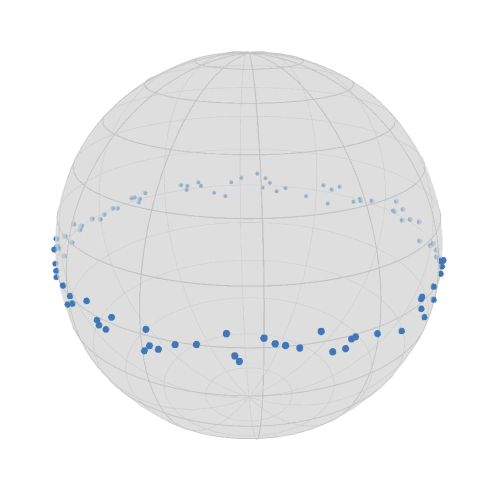
Figure 1: The first three coordinates of the $\mathbb{S}^{6}$-valued 1D synthetic data set defined in eq. 106 projected on $\mathbb{S}^{2}$.

Even though all mappings needed for executing algorithms 1, 2 and 3 are provided in Manifolds.jl [2], it is worth highlighting that we can construct the diagonalizing orthonormal basis at some point $\mathbf{p}\in\mathbb{S}^{6}$ [3] of the form eq. 83 by choosing $(\theta^{j_{1}}_{\mathbf{p}})_{1}:=\frac{\log_{\mathbf{p}}\mathbfcal{X}_{j_{1}}}{\|\log_{\mathbf{p}}\mathbfcal{X}_{j_{1}}\|_{\mathbf{p}}}\in\mathcal{T}_{\mathbf{p}}\mathbb{S}^{6}$ and complete this to an orthonormal basis $\{(\theta^{j_{1}}_{\mathbf{p}})_{1},\ldots,(\theta^{j_{1}}_{\mathbf{p}})_{6}\}\subset\mathcal{T}_{\mathbf{p}}\mathbb{S}^{6}$. The corresponding eigenvalues are then given by

$$\kappa_{j_{1},j}=\left\{\begin{matrix}0,&\text{if $j=1$},\\ d_{\mathbb{S}^{6}}(\mathbf{p},\mathbfcal{X}_{j_{1}})^{2},&\text{if $j\neq 1$}.\end{matrix}\right.$$ (107)

Next, in the Euclidean case a natural choice for the base point $\mathbf{p}$ would be the mean of the data set. This can be generalized in the manifold setting by passing to the Riemannian barycentre, but as noted in work such as [47] this can be problematic in the case of spherical data. Indeed, for the data set defined in eq. 106 the barycentre will be close to a pole of $\mathbb{S}^{6}$ and the data will look 2-dimensional rather than 1-dimensional as fig. 1 suggests. For getting intuition for how the proposed methods behave in both problematic and non-problematic choices of base point we will take a closer look at this behavior by considering two base points. That is, we consider

$$\mathbf{p}^{1}:=\hat{\mathbf{p}}^{1}\in\operatorname*{argmin}_{\mathbf{p}\in\mathbb{S}^{6}}\sum_{i=1}^{100}d_{\mathbb{S}^{6}}(\mathbf{p},\mathbfcal{X}_{i})^{2},\quad\text{and}\quad\mathbf{p}^{2}:=\hat{\mathbf{p}}^{2}\in\operatorname*{argmin}_{\mathbf{p}\in\mathbfcal{X}}\sum_{i=1}^{100}d_{\mathbb{S}^{6}}(\mathbf{p},\mathbfcal{X}_{i})^{2}.$$ (108)

So now given the manifold-valued tensor $\mathbfcal{X}\in(\mathbb{S}^{6})^{100}$ and base points $\mathbf{p}^{1},\mathbf{p}^{2}\in\mathbb{S}^{6}$, we compare algorithms 1, 2 and 3 in terms of global-geometry awareness and computational feasibility. For the former we will consider the relative error eq. 103 for all ranks except full rank, i.e., $r\in\{1,\ldots,5\}$, and compare these to the zero-$\delta$ lower bound. For the latter, we consider the averaged run times for all ranks using the @benchmark macro as mentioned above. Algorithms 1 and 2 do not need extra parameters, but algorithm 3 needs a stopping criterion and a step size. For a fair comparison, we pick the largest step size – up to a factor 2 – under which the iterates converge. This gives $\tau_{1}=2^{-6}=1/64$ and $\tau_{2}=2^{-4}=1/16$. We let the algorithm run until the mild relative gradient condition $\|\nabla g(\mathbfcal{V}^{\ell})\|_{2}/\|\nabla g(\mathbfcal{V}^{0})\|_{2}<10^{-2}$ is satisfied. Finally and additionally, to check whether the curvature corrected approximation error really is a good proxy for the global approximation error on $\mathbb{S}^{6}$ we will also consider the relative discrepancy.

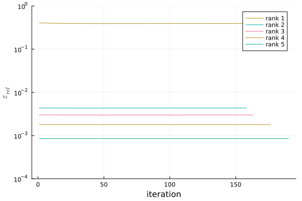
(a)

(b)

Figure 9: The progressions of the relative error (a) of algorithm 3 with different approximation rank until convergence and (b) of algorithms 1, 2 and 3 for an increasing approximation rank of the 1D data on $\mathbb{S}^{6}$ from eq. 106, linearized at $\mathbf{p}_{1}$ from eq. 108. Both y-axes are scaled logarithmically.

The relative error and the relative discrepancy results for low rank approximation at $\mathbf{p}_{1}$ and $\mathbf{p}_{2}$ are shown in figs. 2 and 3. The averaged run times are provided in tables 1 and 2 We note that MC-tSVD converges and we refer the reader for more details to the convergence plots in figs. 9(a) and 10(a) in appendix A.

Low rank approximation at $\mathbf{p}_{1}\in\mathbb{S}^{6}$.

The relative error results in fig. 2(a) are in line with our expectations, i.e., that both CC-tSVD and MC-tSVD pick up on the global geometry better than tSVD, although it has to be emphasized that the difference is minor and is only really visible for rank 1 approximation. This was indeed to be expected, as the effect of positive curvature on the global approximation error is less detrimental than the effect of negative curvature according to theorem 3.4. The figure also confirms that even though the data has rank 1 for a point on the equator, it looks like a rank-2 data set from $\mathbf{p}_{1}$. More interestingly, the results do not come close to the zero-$\delta$ lower bound, which very likely because of the lower bound being overly optimistic. Indeed, having already one point far away from the base point will give a large $\kappa$ – as can be seen in eq. 107 –, and subsequently will give an unrealistically low $\beta(\kappa_{\max})$-value in the lower bound eq. 45. Moving on, the relative discrepancy in fig. 2(b) makes an encouraging case for the accuracy of theorem 3.4. Indeed, we know that $\delta_{rel}(r)\in\mathcal{O}(1)$. Now, the figure suggests that the constant is very small. In other words, the curvature corrected approximation error is global-geometry aware for positive curvature symmetric Riemannian manifolds.

Finally, table 1 tells us that the proposed CC-tSVD algorithm is not only global-geometry aware, but also computationally efficient. Indeed, the CC-tSVD run time is similar to that of tSVD, whereas only one iteration of MC-tSVD already takes up more time. It should be noted here that all three algorithms are implemented in a similar way, e.g., using the same type of vectorization and memory allocation. So these discrepancies are very likely caused by the gradients in algorithm 3 being more expensive to compute, possibly due to the extra 100 logarithmic and exponential map evaluations and the additional 600 parallel transport evaluations per gradient call.

(a)

(b)

Figure 2: The progressions of the relative error (a) and the relative discrepancy (b) of algorithms 1, 2 and 3 for an increasing approximation rank of 1D data on $\mathbb{S}^{6}$, linearized at $\mathbf{p}_{1}$ from eq. 108. (a) suggests that positive curvature does not deteriorate the tSVD approximation, but shows that CC-tSVD and MC-tSVD attain lower errors through picking up on global geometry. (b) shows that discrepancy between the curvature corrected approximation error and the exact global approximation error is very tight, supporting the accuracy of theorem 3.4.

Table 1: The average run times in seconds of algorithms 1, 2 and 3 per approximation rank of 1D data on $\mathbb{S}^{6}$ linearized at $\mathbf{p}_{1}$ from eq. 108. tSVD and CC-tSVD have similar runtimes, but MC-tSVD is significantly slower.

Method	$\operatorname{rank}=1$	$\operatorname{rank}=2$	$\operatorname{rank}=3$	$\operatorname{rank}=4$	$\operatorname{rank}=5$
tSVD	$0.0008435$	$0.0007377$	$0.0008345$	$0.001223$	$0.00087$
CC-tSVD (proposed)	$0.00193$	$0.002363$	$0.002367$	$0.002722$	$0.002932$
MC-tSVD (1 iteration)	$0.00629$	$0.006916$	$0.00837$	$0.00856$	$0.008385$
MC-tSVD	$0.3813$	$0.3687$	$0.3984$	$0.4485$	$0.508$

Low rank approximation at $\mathbf{p}_{2}\in\mathbb{S}^{6}$.

Most of the discussion on low rank approximation at $\mathbf{p}_{1}$ in terms of global-geometry awareness applies to $\mathbf{p}_{2}$. That is, even though the positive curvature is again not strongly deteriorating the naive tSVD approximation, both CC-tSVD and MC-tSVD do pick up on the global geometry slightly better than the naive method for the rank-1 approximation (fig. 3(a)). For the remaining ranks CC-tHOSVD performs slightly worse, i.e., even compared to tSVD. The latter observation is most likely due to an increase in the – still very small – relative discrepancy (fig. 3(b)) compared to the $\mathbf{p}_{1}$ case (fig. 2(b)). This increase makes it more challenging to get a very accurate correction for already almost-zero loss. However, in practice these rank-2 through rank-5 cases are less important than the rank-1 case. So overall, the curvature corrected approximation error does well once again in terms of global-geometry awareness for positive curvature symmetric Riemannian manifolds.

Regarding computational feasibility, we also observe the same as before. That is, table 2 shows that tSVD and CC-tSVD have similar run times and MC-tSVD is significantly slower.

(a)

(b)

Figure 3: The progressions of the relative error (a) and the relative discrepancy (b) of algorithms 1, 2 and 3 for an increasing approximation rank of 1D data on $\mathbb{S}^{6}$, linearized at $\mathbf{p}_{2}$ from eq. 108. (a) shows that CC-tSVD and MC-tSVD attain slightly lower – but similar – errors through picking up on global geometry for rank 1. For higher ranks both tSVD and MC-tSVD perform slightly better. (b) shows that discrepancy between the curvature corrected approximation error and the exact global approximation error is less tight than in fig. 2, which is the likely cause of the difference in performance for the higher rank cases as a more accurate approximation is likely needed.

Table 2: The average run times in seconds of algorithms 1, 2 and 3 per approximation rank of 1D data on $\mathbb{S}^{6}$ linearized at $\mathbf{p}_{2}$ from eq. 108. Similarly as in table 2 tSVD and CC-tSVD are much faster than MC-tSVD.

Method	$\operatorname{rank}=1$	$\operatorname{rank}=2$	$\operatorname{rank}=3$	$\operatorname{rank}=4$	$\operatorname{rank}=5$
tSVD	$0.0008183$	$0.0008283$	$0.0009403$	$0.0008883$	$0.000927$
CC-tSVD (proposed)	$0.001951$	$0.002422$	$0.002525$	$0.003294$	$0.003426$
MC-tSVD (1 iteration)	$0.00653$	$0.00752$	$0.00781$	$0.008286$	$0.00883$
MC-tSVD	$0.2112$	$1.524$	$1.911$	$2.178$	$1.934$

Low rank approximation on $(\mathbb{S}^{6})^{100}$.

Overall, the above results strongly support our claim that CC-tSVD is a good compromise between global-geometry awareness and computational feasibility in the case of positive curvature. That is, compared to tSVD, which is fast but not global-geometry aware, and compared to MC-tSVD, which is global-geometry aware but slow. It should be emphasized once more that the relative errors are very comparable, which is to be expected as curvature effects due to positive curvature are less of a problem than those due to negative curvature according to theorem 3.4. Next, we will get a better idea to what extent the proposed method can account for the more problematic case of negative curvature.

6.1.2 Symmetric positive definite matrix data.

Next, we move on to $\mathcal{P}(3)$ – which is a symmetric manifold under the bi-invariant metric – and consider the order-1 manifold-valued tensor $\mathbfcal{X}^{\prime}\in(\mathcal{P}(3))^{100}$ defined entry-wise as

$$\mathbfcal{X}^{\prime}_{i}:=\exp_{I_{3}}(\tau_{i}\begin{pmatrix}0&0&0\\ 0&1&0\\ 0&0&0\\ \end{pmatrix}),\quad\tau_{i}\sim\mathcal{N}(0,2),\;i=1,\ldots,100,$$ (109)

and $\mathbfcal{X}\in\mathcal{P}(3)^{100}$ defined entry-wise as

$$\mathbfcal{X}_{i}:=\exp_{\mathbfcal{X}^{\prime}_{i}}(\eta_{\mathbfcal{X}^{\prime}_{i}}^{i}),\quad\text{where }\eta_{\mathbfcal{X}^{\prime}_{i}}^{i}\in\mathcal{T}_{\mathbfcal{X}^{\prime}_{i}}\mathcal{P}(3)\text{ is a centered Gaussian random tangent vector with variance $0.05$.}$$ (110)

A subset of this data set is visualized in fig. 4, from which it is clear that the data set has rank 1.

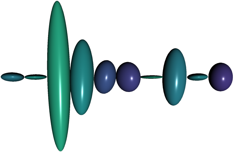
Figure 4: A visualization of the 1D $\mathcal{P}(3)$-valued data set defined in eq. 110.

Again, for the sake of completeness, it is worth highlighting that we can construct the diagonalizing orthonormal basis at some point $\mathbf{p}\in\mathcal{P}(3)$ [3] of the form eq. 83 by first considering the eigendecomposition of $\frac{\log_{\mathbf{p}}\mathbfcal{X}_{j_{1}}}{\|\log_{\mathbf{p}}\mathbfcal{X}_{j_{1}}\|_{\mathbf{p}}}\in\mathcal{T}_{\mathbf{p}}\mathcal{P}(3)$, which is a symmetric $3\times 3$ matrix, i.e.,

$$\frac{\log_{\mathbf{p}}\mathbfcal{X}_{j_{1}}}{\|\log_{\mathbf{p}}\mathbfcal{X}_{j_{1}}\|_{\mathbf{p}}}=\sum_{k}^{3}\lambda_{k}^{j_{1}}\mathbf{v}_{k}^{j_{1}}(\mathbf{v}_{k}^{j_{1}})^{\top}.$$ (111)

Next, defining the index set

$$\mathcal{J}:=\{j=(k,l)\>\mid\>k=1,\dots,3,\;l=k,\ldots,3\},$$ (112)

we obtain an orthonormal basis $\{(\theta^{j_{1}}_{\mathbf{p}})_{(1,1)},(\theta^{j_{1}}_{\mathbf{p}})_{(1,2)},(\theta^{j_{1}}_{\mathbf{p}})_{(1,3)},(\theta^{j_{1}}_{\mathbf{p}})_{(2,2)},(\theta^{j_{1}}_{\mathbf{p}})_{(2,3)},(\theta^{j_{1}}_{\mathbf{p}})_{(3,3)}\}\subset\mathcal{T}_{\mathbf{p}}\mathcal{P}(3)$ given by

$$(\theta^{j_{1}}_{\mathbf{p}})_{j}:=\left\{\begin{matrix}\frac{1}{2}(\mathbf{v}^{j_{1}}_{k}(\mathbf{v}^{j_{1}}_{l})^{\top}+\mathbf{v}_{l}^{j_{1}}(\mathbf{v}_{k}^{j_{1}})^{\top}),&j=(k,l)\in\mathcal{J}&\text{if $k=l$},\\ \frac{1}{\sqrt{2}}(\mathbf{v}_{k}^{j_{1}}(\mathbf{v}_{l}^{j_{1}})^{\top}+\mathbf{v}_{l}^{j_{1}}(\mathbf{v}_{k}^{j_{1}})^{\top}),&j=(k,l)\in\mathcal{J}&\text{if $k\neq l$},\end{matrix}\right..$$ (113)

The corresponding eigenvalues are then given by

$$\kappa_{j_{1},j}=-\frac{1}{4}(\lambda_{k}^{j_{1}}-\lambda_{l}^{j_{1}})^{2}d_{\mathcal{P}(3)}(\mathbf{p},\mathbfcal{X}_{j_{1}})^{2},\quad j=(k,l)\in\mathcal{J}.$$ (114)

Unlike the spherical case, we do not expect problematic behavior from picking the base point as the barycentre of the data. That is, we consider

$$\mathbf{p}:=\operatorname*{argmin}_{\mathbf{p}\in\mathcal{P}(3)}\sum_{i=1}^{100}d_{\mathcal{P}(3)}(\mathbf{p},\mathbfcal{X}_{i})^{2}.$$ (115)

Note that we do indeed get a unique minimizer due to the fact that the barycentre problem is strongly geodesically convex on the Hadamard manifold $\mathcal{P}(3)$.

We will run the same experimental setup as for spherical data. That is, we use the same stopping criterion for algorithm 3 as before and again use the largest step size – up to a factor – that does not result in a diverging solver, which is $\tau=2^{-16}$.

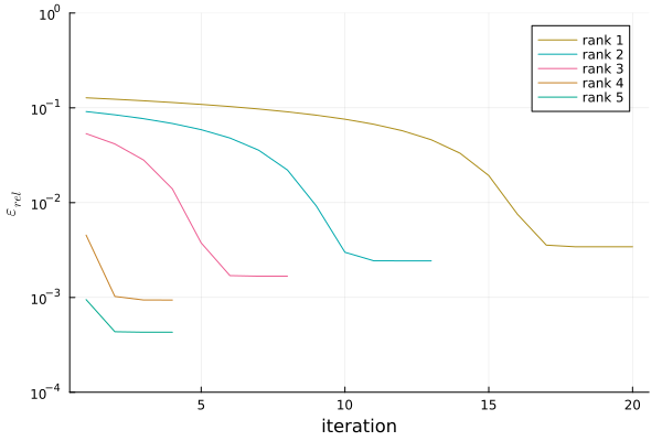
(a)

(b)

Figure 11: The progressions of the relative error (a) of algorithm 3 with different approximation rank until convergence and (b) of algorithms 1, 2 and 3 for an increasing approximation rank of the 1D data on $\mathcal{P}(3)$ from eq. 110, linearized at $\mathbf{p}$ from eq. 115. Both y-axes are scaled logarithmically.

The relative error and the relative discrepancy results for low rank approximation at $\mathbf{p}$ are shown in fig. 5. The averaged run times are provided in table 3. We note that MC-tSVD converges and we refer the reader for more details to the convergence plots in fig. 11(a) in appendix A.

Low rank approximation at $\mathbf{p}\in\mathcal{P}(3)$.

For the data set in eq. 110 the effect of curvature is more clearly pronounced than for the positive curvature case. Indeed, there is a large difference between the relative errors of tSVD and those of CC-tSVD and MC-tSVD (fig. 5(a)). Moreover, both CC-tSVD and MC-tSVD almost reach the zero-$\delta$ lower bound, which makes a strong case for the global-geometry awareness of CC-tSVD for symmetric Riemannian manifolds with negative curvature. This also suggests that the lower bound is actually reasonably tight in the negative curvature case, contrary to the positive curvature case. Additional evidence of the global-geometry awareness of CC-tSVD follows from fig. 5(b), which also suggests that the constant we expect from $\delta_{rel}(r)\in\mathcal{O}(1)$ is once again very small. Summarized, we conclude that the curvature corrected approximation error and CC-tSVD are global-geometry aware for negative curvature as well.

Regarding computational feasibility, we make similar observations as for the positive curvature case. That is, table 3 shows that tSVD and CC-tSVD have similar run times and MC-tSVD is on average more than an order of magnitude slower.

(a)

(b)

Figure 5: The progressions of the relative error (a) and the relative discrepancy (b) of algorithms 1, 2 and 3 for an increasing approximation rank of 1D data on $\mathcal{P}(3)$, linearized at $\mathbf{p}$ from eq. 115. (a) shows that CC-tSVD and MC-tSVD attain significantly lower errors through picking up on global geometry for all ranks. (b) shows that discrepancy between the curvature corrected approximation error and the exact global approximation error is very tight, supporting again the accuracy of theorem 3.4.

Table 3: The average run times in seconds of algorithms 1, 2 and 3 per approximation rank of 1D data on $\mathcal{P}(3)$ linearized at $\mathbf{p}$ from eq. 115. Similarly to tables 1 and 2 tSVD and CC-tSVD are much faster than MC-tSVD.

Method	$\operatorname{rank}=1$	$\operatorname{rank}=2$	$\operatorname{rank}=3$	$\operatorname{rank}=4$	$\operatorname{rank}=5$
tSVD	$0.01811$	$0.01816$	$0.0177$	$0.02174$	$0.01868$
CC-tSVD (proposed)	$0.03735$	$0.0394$	$0.04367$	$0.05252$	$0.05743$
MC-tSVD (1 iteration)	$0.1534$	$0.1726$	$0.1981$	$0.2029$	$0.2186$
MC-tSVD	$1.091$	$0.933$	$0.5923$	$0.3997$	$0.424$

Low rank approximation on $\mathcal{P}(3)^{100}$.

Overall, the above results also strongly support our claim that CC-tSVD is a good compromise between global-geometry awareness and computational feasibility in the case of positive curvature. It should be emphasized this time that the relative errors between the naive tSVD and CC-tSVD is very significant due to the negative curvature, but that the difference between MC-tSVD and CC-tSVD is very slight.

6.2 Real 2D DT-MRI data.

An important application of $\mathcal{P}(3)$-valued data processing is in diffusion tensor magnetic resonance imaging (DT-MRI). In the following, we apply the proposed CC-tHOSVD on a DT-MRI data set of a human head from the Camino project [21] and compare performance with the naive tHOSVD.

The Camino data set gives us a manifold-valued tensor in $\mathbfcal{X}^{\prime}\in\mathcal{P}(3)^{112\times 112\times 50}$ of order 3. From this manifold-valued tensor, we construct two manifold-valued tensors of order 2. That is, we construct the manifold-valued tensors $\mathbfcal{X}\in\mathcal{P}(3)^{40\times 40}$ and $\mathbfcal{X}^{patch}\in\mathcal{P}(3)^{10\times 10}$ defined as

$$\mathbfcal{X}:=\mathbfcal{X}^{\prime}_{38:77,36:75,15},\quad\mathbfcal{X}^{patch}:=\mathbfcal{X}^{\prime}_{38:47,36:45,15}=\mathbfcal{X}_{1:10,1:10}.$$ (116)

Both data sets are visualized in fig. 6.

(a)

(b)

Figure 6: A visualization of the 2D $\mathcal{P}(3)$-valued slices $\mathbfcal{X}\in\mathcal{P}(3)^{40\times 40}$ and $\mathbfcal{X}^{patch}\in\mathcal{P}(3)^{10\times 10}$ of DT-MRI data from the Camino project [21]. Note that (b) is the lower left $10\times 10$ patch of (a).

The curvature tensor diagonalizing orthonormal basis at some point $\mathbf{p}\in\mathcal{P}(3)$ of the form eq. 83 can be constructed analogously to the construction in section 6.1.2. Also analogously to above, we pick each data’s respective barycentre as the base point for the low multi-linear rank approximation.

For exploring the behavior of the relative error and the relative discrepancy for approximating $\mathbfcal{X}$ we compute a multi-linear rank-$(r,r)$ approximation using algorithms 1 and 2 for $r$ ranging from 1 to 40 with intervals of 3. For the run time comparison, we take a coarser partition and use intervals of 7. Subsequently, for $\mathbfcal{X}^{patch}$ we compute a multi-linear rank-$(r,r)$ approximation for all $r$ from 1 to 9, i.e., except full rank. For the run time comparison, only the odd ranks are benchmarked.

The relative error and the relative discrepancy results for low multi-linear rank-$(r,r)$ approximation of $\mathbfcal{X}$ and $\mathbfcal{X}^{patch}$ are shown in figs. 7 and 8 respectively. The averaged run times are provided in tables 4 and 5.

Low multi-linear rank approximation on $\mathcal{P}(3)^{40\times 40}$.

The data set in fig. 6(a) is clearly testing the limits of the CC-tHOSVD now that the data set does not have a low multi-linear rank, unlike the 1D examples from above. In particular, as a large relative error at multi-linear rank $(1,1)$ goes hand in hand with large tangent space error, the discrepancy between curvature approximation error and the global approximation error in theorem 3.4 is large. This leaves CC-tHOSVD unable to take the global geometry into account and results in a worse relative error than that of tHOSVD (Figure 7(a)). However, for larger approximation rank, the error naturally decreases and CC-tHOSVD once again picks up on the global geometry and reaches the zero-$\delta$ lower bound. The latter claim is also supported by the relative discrepancy in fig. 7(b) that decreases to a small value, indicating that the constant we expect from $\delta_{rel}(r)\in\mathcal{O}(1)$ is once again very small.

Regarding computational feasibility, we observe that the run time increases quadratically in the approximation rank (table 4), or equivalently linearly in the core tensor size. Quadratic scaling indicates that the bottleneck is the construction of the real-valued tensor $\mathbfcal{B}$ from eq. 85 and not computing $\mathbfcal{A}$ from eq. 86 – which would scale with a fourth power in the approximation rank or quadratically in the core tensor size – or solving the linear system – which would scale with a sixth power in rank and cubically in the core tensor size. In other words, this would not be resolved by passing to MC-tHOSVD, which is – similarly to the 1D case – even slower due to the additional logarithmic map, exponential map and parallel transport calls.

So overall, CC-tHOSVD remains to be – even in the current implementation – a good compromise between global-geometry awareness and computational feasibility.

(a)

(b)

Figure 7: The progressions of the relative error (a) and the relative discrepancy (b) of algorithms 1 and 2 for an increasing approximation rank of the $40\times 40$ $\mathcal{P}(3)$-valued tensor linearized at the data barycentre. (a) shows that CC-tHOSVD gruadually picks up on the global geometry as the relative error decreases, and in doing so attains better estimates for higher ranks. (b) shows that discrepancy between the curvature corrected approximation error and the exact global approximation error is very tight, supporting again the accuracy of theorem 3.4.

Table 4: The average run times in seconds of algorithms 1 and 2 per multi-linear approximation rank of the $40\times 40$ Camino slice data on $\mathcal{P}(3)$ linearized at the data barycentre. The run time of CC-tHOSVD increases approximately quadratically with the rank.

Method	$\operatorname{rank}=1$	$\operatorname{rank}=8$	$\operatorname{rank}=15$	$\operatorname{rank}=22$	$\operatorname{rank}=29$	$\operatorname{rank}=36$
tHOSVD	$0.2888$	$0.4062$	$0.4438$	$0.6294$	$0.9385$	$0.969$
CC-tHOSVD (proposed)	$0.4683$	$6.93$	$24.92$	$53.28$	$99.06$	$157.8$

Low multi-linear rank approximation on $\mathcal{P}(3)^{10\times 10}$.

The data set in fig. 6(b) on the other hand behaves similarly to the 1D example in section 6.1.2. That is, for all approximation ranks the relative error reaches the zero-$\delta$ lower bound and the relative discrepancy (fig. 8(b)) is very low at all times. Combined, these two observations indicate strong global-geometry awareness. Note that it is unsurprising that patch-wise compression of images works better than global compression as attempted above. That is, because the image’s pixels tend to vary little on a local scale, but typically vary significantly when considered globally.

Regarding the run times in table 5, we observe quadratic scaling in rank once again, but note that this time the difference to tHOSVD is much more managable.

So, also for this data set we conclude that CC-tHOSVD is a good compromise between global-geometry awareness and computational feasibility.

(a)

(b)

Figure 8: The progressions of the relative error (a) and the relative discrepancy (b) algorithms 1 and 2 for an increasing approximation rank of the $10\times 10$ $\mathcal{P}(3)$-valued tensor linearized at the data barycentre. (a) shows that CC-tHOSVD attains significantly lower errors through picking up on global geometry for all ranks. (b) shows that discrepancy between the curvature corrected approximation error and the exact global approximation error is very tight, supporting again the accuracy of theorem 3.4.

Table 5: The average run times in seconds of algorithms 1 and 2 per approximation rank of the $10\times 10$ Camino slice data on $\mathcal{P}(3)$ linearized at the data barycentre. The run time of CC-tHOSVD increases approximately quadratically with the rank.

Method	$\operatorname{rank}=1$	$\operatorname{rank}=3$	$\operatorname{rank}=5$	$\operatorname{rank}=7$	$\operatorname{rank}=9$
tHOSVD	$0.00768$	$0.009575$	$0.00896$	$0.00959$	$0.010315$
CC-tHOSVD (proposed)	$0.02036$	$0.08746$	$0.1853$	$0.3186$	$0.5483$

7 Conclusions.

In this work we set out to construct a general framework for tangent space-based approximation of manifold-valued tensors that is applicable to general Riemannian manifolds, global-geometry aware and computationally feasible.

General applicability.

Through focusing on symmetric Riemannian manifolds – covering a large class of manifolds that are being used in many practical settings – we were able to show that the leading term of the global approximation error eq. 1 – the curvature corrected approximation error – is fully determined by the tangent space approximation error and the curvature at the point of linearization.

Global-geometry awareness.

Subsequently, we showed that minimizing this curvature corrected approximation error – already giving us general applicability – instead of the global approximation error also gives us global-geometry awareness. In particular, we showed that under mild conditions minimizing the curvature corrected approximation error diminishes the discrepancy with the global approximation error. In other words, minimizers of the curvature corrected approximation error based methods will have a low global approximation error. Moreover and under mild conditions on the set of admissible approximators, we showed that as curvature effects vanish, minimizers of the curvature corrected approximation error converge to the minimizer of the zero-curvature case, i.e., the naive uncorrected tangent space-based approach.

Computational feasibility.

These latter observations were a strong motivation to consider numerical schemes that are initialized from naive tangent space-based methods and that are corrected for curvature from thereon. In particular, in a case study on low multi-linear rank approximation we used such a strategy and proposed the curvature corrected truncated higher-order singular value decomposition (CC-tHOSVD) scheme along with a generalization of the (truncated) HOSVD and metric-corrected tHOSVD (MC-tHOSVD) as a baseline approach that minimizes the global approximation error for benchmarking. The CC-tHOSVD – already considerate of general applicability and global-geometry awareness by construction – was constructed to account for computational feasibility through its main step being to solve a linear system, whose matrix representation is symmetric positive semi-definite and is positive definite under mild conditions.

Finally, in numerical experiments on synthetic and real tensor-valued data living in symmetric Riemannian manifolds that cover the cases of both positive and negative curvature, we tested the algorithm’s performance and conclude that CC-tHOSVD is indeed generally applicable, global-geometry aware and computationally feasible.

Appendix A Supplementary results from section 6.

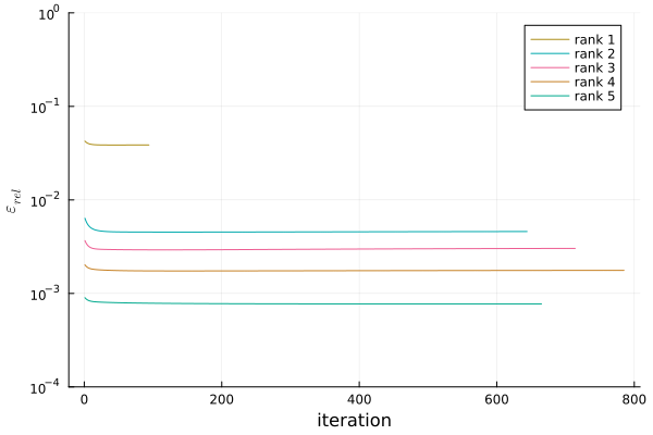
(a)

(b)

Figure 10: The progressions of the relative error (a) of algorithm 3 with different approximation rank until convergence and (b) of algorithms 1, 2 and 3 for an increasing approximation rank of the 1D data on $\mathbb{S}^{6}$ from eq. 106, linearized at $\mathbf{p}_{2}$ from eq. 108. Both y-axes are scaled logarithmically.

(a)

(b)

Figure 12: The progressions of the relative error of algorithms 1 and 2 for an increasing approximation rank of (a) the $40\times 40$ $\mathcal{P}(3)$-valued tensor and of (b) the $10\times 10$ $\mathcal{P}(3)$-valued tensor from eq. 116, both of which are linearized at the data barycentre. Both y-axes are scaled logarithmically.

References

- [1] Brent L Adams, Stuart I Wright, and Karsten Kunze. Orientation imaging: the emergence of a new microscopy. Metallurgical Transactions A, 24(4):819–831, 1993.
- [2] Seth D Axen, Mateusz Baran, Ronny Bergmann, and Krzysztof Rzecki. Manifolds. jl: an extensible julia framework for data analysis on manifolds. arXiv preprint arXiv:2106.08777, 2021.
- [3] Miroslav Bacák, Ronny Bergmann, Gabriele Steidl, and Andreas Weinmann. A second order nonsmooth variational model for restoring manifold-valued images. SIAM Journal on Scientific Computing, 38(1):A567–A597, 2016.
- [4] Peter J Basser, James Mattiello, and Denis LeBihan. Mr diffusion tensor spectroscopy and imaging. Biophysical journal, 66(1):259–267, 1994.
- [5] Ronny Bergmann. Manopt. jl: Optimization on manifolds in julia. Journal of Open Source Software, 7(70):3866, 2022.
- [6] Ronny Bergmann and Pierre-Yves Gousenbourger. A variational model for data fitting on manifolds by minimizing the acceleration of a bézier curve. Frontiers in Applied Mathematics and Statistics, 4, 2018.
- [7] Ronny Bergmann, Roland Herzog, Maurício Silva Louzeiro, Daniel Tenbrinck, and José Vidal-Núñez. Fenchel duality theory and a primal-dual algorithm on riemannian manifolds. Foundations of Computational Mathematics, 21(6):1465–1504, 2021.
- [8] Ronny Bergmann, Friederike Laus, Johannes Persch, and Gabriele Steidl. Recent advances in denoising of manifold-valued images. Handbook of Numerical Analysis, 20:553–578, 2019.
- [9] Ronny Bergmann, Johannes Persch, and Gabriele Steidl. A parallel douglas–rachford algorithm for minimizing rof-like functionals on images with values in symmetric hadamard manifolds. SIAM Journal on Imaging Sciences, 9(3):901–937, 2016.
- [10] William M Boothby and William Munger Boothby. An introduction to differentiable manifolds and Riemannian geometry, Revised, volume 120. Gulf Professional Publishing, 2003.
- [11] Andrea Braides. A handbook of -convergence. In Handbook of Differential Equations: stationary partial differential equations, volume 3, pages 101–213. Elsevier, 2006.
- [12] Michael M Bronstein, Joan Bruna, Yann LeCun, Arthur Szlam, and Pierre Vandergheynst. Geometric deep learning: going beyond euclidean data. IEEE Signal Processing Magazine, 34(4):18–42, 2017.
- [13] Deng Cai, Xiaofei He, Xiaoyun Wu, and Jiawei Han. Non-negative matrix factorization on manifold. In 2008 eighth IEEE international conference on data mining, pages 63–72. IEEE, 2008.
- [14] HanQin Cai, Keaton Hamm, Longxiu Huang, and Deanna Needell. Mode-wise tensor decompositions: Multi-dimensional generalizations of cur decompositions. J. Mach. Learn. Res., 22:185–1, 2021.
- [15] Manfredo Perdigao do Carmo. Riemannian geometry. Birkhäuser, 1992.
- [16] J Douglas Carroll and Jih-Jie Chang. Analysis of individual differences in multidimensional scaling via an n-way generalization of “eckart-young” decomposition. Psychometrika, 35(3):283–319, 1970.
- [17] Raymond B Cattell. “parallel proportional profiles” and other principles for determining the choice of factors by rotation. Psychometrika, 9(4):267–283, 1944.
- [18] Raymond B Cattell. The three basic factor-analytic research designs—their interrelations and derivatives. Psychological bulletin, 49(5):499, 1952.
- [19] Rudrasis Chakraborty, Dohyung Seo, and Baba C Vemuri. An efficient exact-pga algorithm for constant curvature manifolds. In Proceedings of the IEEE conference on computer vision and pattern recognition, pages 3976–3984, 2016.
- [20] Tony F Chan, Sung Ha Kang, and Jianhong Shen. Total variation denoising and enhancement of color images based on the cb and hsv color models. Journal of Visual Communication and Image Representation, 12(4):422–435, 2001.
- [21] Philip A Cook, Yu Bai, Matt G Hall, Shahrum Nedjati-Gilani, Kiran K Seunarine, and Daniel C Alexander. Camino: Diffusion mri reconstruction and processing. 2005.
- [22] Calin Cruceru, Gary Bécigneul, and Octavian-Eugen Ganea. Computationally tractable riemannian manifolds for graph embeddings. In Proceedings of the AAAI Conference on Artificial Intelligence, volume 35, pages 7133–7141, 2021.
- [23] Charles Curry, Stephen Marsland, and Robert I McLachlan. Principal symmetric space analysis. Journal of Computational Dynamics, 6(2):251–276, 2019.
- [24] James Damon and JS Marron. Backwards principal component analysis and principal nested relations. Journal of Mathematical Imaging and Vision, 50(1-2):107–114, 2014.
- [25] Lieven De Lathauwer, Bart De Moor, and Joos Vandewalle. A multilinear singular value decomposition. SIAM journal on Matrix Analysis and Applications, 21(4):1253–1278, 2000.
- [26] Willem Diepeveen and Jan Lellmann. An inexact semismooth newton method on riemannian manifolds with application to duality-based total variation denoising. SIAM Journal on Imaging Sciences, 14(4):1565–1600, 2021.
- [27] P Thomas Fletcher, Conglin Lu, and Sarang Joshi. Statistics of shape via principal geodesic analysis on lie groups. In 2003 IEEE Computer Society Conference on Computer Vision and Pattern Recognition, 2003. Proceedings., volume 1, pages I–I. IEEE, 2003.
- [28] P Thomas Fletcher, Conglin Lu, Stephen M Pizer, and Sarang Joshi. Principal geodesic analysis for the study of nonlinear statistics of shape. IEEE transactions on medical imaging, 23(8):995–1005, 2004.
- [29] Yifan Fu, Junbin Gao, Xia Hong, and David Tien. Low rank representation on riemannian manifold of symmetric positive definite matrices. In Proceedings of the 2015 SIAM International Conference on Data Mining, pages 316–324. SIAM, 2015.
- [30] Philipp Grohs and Johannes Wallner. Definability and stability of multiscale decompositions for manifold-valued data. Journal of the Franklin Institute, 349(5):1648–1664, 2012.
- [31] Albert Gu, Frederic Sala, Beliz Gunel, and Christopher Ré. Learning mixed-curvature representations in product spaces. In International Conference on Learning Representations, 2019.
- [32] Naiyang Guan, Dacheng Tao, Zhigang Luo, and Bo Yuan. Manifold regularized discriminative nonnegative matrix factorization with fast gradient descent. IEEE Transactions on Image Processing, 20(7):2030–2048, 2011.
- [33] Ghassan Hamarneh, Chris McIntosh, and Mark S Drew. Perception-based visualization of manifold-valued medical images using distance-preserving dimensionality reduction. IEEE transactions on medical imaging, 30(7):1314–1327, 2011.
- [34] Mehrtash T Harandi, Mathieu Salzmann, and Richard Hartley. From manifold to manifold: Geometry-aware dimensionality reduction for spd matrices. In European conference on computer vision, pages 17–32. Springer, 2014.
- [35] Mehrtash T Harandi, Conrad Sanderson, Richard Hartley, and Brian C Lovell. Sparse coding and dictionary learning for symmetric positive definite matrices: A kernel approach. In Computer Vision–ECCV 2012: 12th European Conference on Computer Vision, Florence, Italy, October 7-13, 2012, Proceedings, Part II 12, pages 216–229. Springer, 2012.
- [36] Richard A Harshman et al. Foundations of the parafac procedure: Models and conditions for an" explanatory" multimodal factor analysis. 1970.
- [37] Søren Hauberg. Principal curves on riemannian manifolds. IEEE transactions on pattern analysis and machine intelligence, 38(9):1915–1921, 2015.
- [38] Frank L Hitchcock. The expression of a tensor or a polyadic as a sum of products. Journal of Mathematics and Physics, 6(1-4):164–189, 1927.
- [39] Frank L Hitchcock. Multiple invariants and generalized rank of a p-way matrix or tensor. Journal of Mathematics and Physics, 7(1-4):39–79, 1928.
- [40] Jeffrey Ho, Yuchen Xie, and Baba Vemuri. On a nonlinear generalization of sparse coding and dictionary learning. In International conference on machine learning, pages 1480–1488. PMLR, 2013.
- [41] Jin Huang, Feiping Nie, Heng Huang, and Chris Ding. Robust manifold nonnegative matrix factorization. ACM Transactions on Knowledge Discovery from Data (TKDD), 8(3):1–21, 2014.
- [42] Zhiwu Huang, Jiqing Wu, and Luc Van Gool. Building deep networks on grassmann manifolds. arXiv preprint arXiv:1611.05742, 2016.
- [43] Stephan Huckemann, Thomas Hotz, and Axel Munk. Intrinsic shape analysis: Geodesic pca for riemannian manifolds modulo isometric lie group actions. Statistica Sinica, pages 1–58, 2010.
- [44] Stephan Huckemann and Herbert Ziezold. Principal component analysis for riemannian manifolds, with an application to triangular shape spaces. Advances in Applied Probability, 38(2):299–319, 2006.
- [45] Mark A Iwen, Deanna Needell, Michael Perlmutter, and Elizaveta Rebrova. Modewise operators, the tensor restricted isometry property, and low-rank tensor recovery. arXiv preprint arXiv:2109.10454, 2021.
- [46] Mark A Iwen, Deanna Needell, Elizaveta Rebrova, and Ali Zare. Lower memory oblivious (tensor) subspace embeddings with fewer random bits: modewise methods for least squares. SIAM Journal on Matrix Analysis and Applications, 42(1):376–416, 2021.
- [47] Sungkyu Jung, Ian L Dryden, and James Stephen Marron. Analysis of principal nested spheres. Biometrika, 99(3):551–568, 2012.
- [48] Arie Kapteyn, Heinz Neudecker, and Tom Wansbeek. An approach to n-mode components analysis. Psychometrika, 51:269–275, 1986.
- [49] Martin Keller-Ressel and Stephanie Nargang. Hydra: a method for strain-minimizing hyperbolic embedding of network-and distance-based data. Journal of Complex Networks, 8(1):cnaa002, 2020.
- [50] Henk AL Kiers. Towards a standardized notation and terminology in multiway analysis. Journal of Chemometrics: A Journal of the Chemometrics Society, 14(3):105–122, 2000.
- [51] Tamara G Kolda and Brett W Bader. Tensor decompositions and applications. SIAM review, 51(3):455–500, 2009.
- [52] Dmitri Krioukov, Fragkiskos Papadopoulos, Maksim Kitsak, Amin Vahdat, and Marián Boguná. Hyperbolic geometry of complex networks. Physical Review E, 82(3):036106, 2010.
- [53] Pieter M Kroonenberg and Jan De Leeuw. Principal component analysis of three-mode data by means of alternating least squares algorithms. Psychometrika, 45:69–97, 1980.
- [54] Drew Lazar and Lizhen Lin. Scale and curvature effects in principal geodesic analysis. Journal of Multivariate Analysis, 153:64–82, 2017.
- [55] John M Lee. Smooth manifolds. In Introduction to Smooth Manifolds, pages 1–31. Springer, 2013.
- [56] Weiyang Liu, Yandong Wen, Zhiding Yu, Ming Li, Bhiksha Raj, and Le Song. Sphereface: Deep hypersphere embedding for face recognition. In Proceedings of the IEEE conference on computer vision and pattern recognition, pages 212–220, 2017.
- [57] Federico López, Beatrice Pozzetti, Steve Trettel, Michael Strube, and Anna Wienhard. Symmetric spaces for graph embeddings: A finsler-riemannian approach. In International Conference on Machine Learning, pages 7090–7101. PMLR, 2021.
- [58] Kanti V Mardia, Henrik Wiechers, Benjamin Eltzner, and Stephan F Huckemann. Principal component analysis and clustering on manifolds. Journal of Multivariate Analysis, 188:104862, 2022.
- [59] Didier Massonnet and Kurt L Feigl. Radar interferometry and its application to changes in the earth’s surface. Reviews of geophysics, 36(4):441–500, 1998.
- [60] Nina Miolane, Nicolas Guigui, Alice Le Brigant, Johan Mathe, Benjamin Hou, Yann Thanwerdas, Stefan Heyder, Olivier Peltre, Niklas Koep, Hadi Zaatiti, et al. Geomstats: a python package for riemannian geometry in machine learning. The Journal of Machine Learning Research, 21(1):9203–9211, 2020.
- [61] J Mocks. Topographic components model for event-related potentials and some biophysical considerations. IEEE transactions on biomedical engineering, 35(6):482–484, 1988.
- [62] Maximillian Nickel and Douwe Kiela. Poincaré embeddings for learning hierarchical representations. Advances in neural information processing systems, 30, 2017.
- [63] Victor M Panaretos, Tung Pham, and Zhigang Yao. Principal flows. Journal of the American Statistical Association, 109(505):424–436, 2014.
- [64] Xavier Pennec. Barycentric subspace analysis on manifolds. The Annals of Statistics, 46(6A):2711 – 2746, 2018.
- [65] Xinglin Piao, Yongli Hu, Junbin Gao, Yanfeng Sun, Xin Yang, and Baocai Yin. Reweighted non-convex non-smooth rank minimization based spectral clustering on grassmann manifold. In Proceedings of the Asian Conference on Computer Vision, 2020.
- [66] Inam Ur Rahman, Iddo Drori, Victoria C Stodden, David L Donoho, and Peter Schröder. Multiscale representations for manifold-valued data. Multiscale Modeling & Simulation, 4(4):1201–1232, 2005.
- [67] Salem Said, Nicolas Courty, Nicolas Le Bihan, and Stephen J Sangwine. Exact principal geodesic analysis for data on so (3). In 2007 15th European Signal Processing Conference, pages 1701–1705. IEEE, 2007.
- [68] Takashi Sakai. Riemannian geometry, volume 149. American Mathematical Soc., 1996.
- [69] John W Sammon. A nonlinear mapping for data structure analysis. IEEE Transactions on computers, 100(5):401–409, 1969.
- [70] Zhenqiu Shu, Hongfei Fan, Pu Huang, Dong Wu, Feiyue Ye, and Xiaojun Wu. Multiple laplacian graph regularised low-rank representation with application to image representation. IET Image Processing, 11(6):370–378, 2017.
- [71] Ondrej Skopek, Octavian-Eugen Ganea, and Gary Bécigneul. Mixed-curvature variational autoencoders. In 8th International Conference on Learning Representations (ICLR 2020)(virtual). International Conference on Learning Representations, 2020.
- [72] Stefan Sommer. Horizontal dimensionality reduction and iterated frame bundle development. In International Conference on Geometric Science of Information, pages 76–83. Springer, 2013.
- [73] Stefan Sommer, François Lauze, and Mads Nielsen. Optimization over geodesics for exact principal geodesic analysis. Advances in Computational Mathematics, 40:283–313, 2014.
- [74] Zhao Song, David P Woodruff, and Peilin Zhong. Relative error tensor low rank approximation. In Proceedings of the Thirtieth Annual ACM-SIAM Symposium on Discrete Algorithms, pages 2772–2789. SIAM, 2019.
- [75] Rishi Sonthalia and Anna Gilbert. Tree! i am no tree! i am a low dimensional hyperbolic embedding. Advances in Neural Information Processing Systems, 33:845–856, 2020.
- [76] Puoya Tabaghi, Michael Khanzadeh, Yusu Wang, and Sivash Mirarab. Principal component analysis in space forms. arXiv preprint arXiv:2301.02750, 2023.
- [77] Ledyard R Tucker. Implications of factor analysis of three-way matrices for measurement of change. Problems in measuring change, 15(122-137):3, 1963.
- [78] Ledyard R Tucker. Some mathematical notes on three-mode factor analysis. Psychometrika, 31(3):279–311, 1966.
- [79] Oncel Tuzel, Fatih Porikli, and Peter Meer. Region covariance: A fast descriptor for detection and classification. In Computer Vision–ECCV 2006: 9th European Conference on Computer Vision, Graz, Austria, May 7-13, 2006. Proceedings, Part II 9, pages 589–600. Springer, 2006.
- [80] M Alex O Vasilescu and Demetri Terzopoulos. Multilinear analysis of image ensembles: Tensorfaces. ECCV (1), 2350:447–460, 2002.
- [81] Jörg A Walter. H-mds: a new approach for interactive visualization with multidimensional scaling in the hyperbolic space. Information systems, 29(4):273–292, 2004.
- [82] Boyue Wang, Yongli Hu, Junbin Gao, Muhammad Ali, David Tien, Yanfeng Sun, and Baocai Yin. Low rank representation on spd matrices with log-euclidean metric. Pattern Recognition, 76:623–634, 2018.
- [83] Boyue Wang, Yongli Hu, Junbin Gao, Yanfeng Sun, and Baocai Yin. Low rank representation on grassmann manifolds. In Asian conference on computer vision, pages 81–96. Springer, 2015.
- [84] Richard C Wilson, Edwin R Hancock, Elżbieta Pekalska, and Robert PW Duin. Spherical and hyperbolic embeddings of data. IEEE transactions on pattern analysis and machine intelligence, 36(11):2255–2269, 2014.
- [85] Chun-Hao Yang and Baba C Vemuri. Nested grassmanns for dimensionality reduction with applications to shape analysis. In Information Processing in Medical Imaging: 27th International Conference, IPMI 2021, Virtual Event, June 28–June 30, 2021, Proceedings 27, pages 136–149. Springer, 2021.
- [86] Zhigang Yao, Benjamin Eltzner, and Tung Pham. Principal sub-manifolds. arXiv preprint arXiv:1604.04318, 2016.
- [87] Ming Yin, Junbin Gao, and Yi Guo. Nonlinear low-rank representation on stiefel manifolds. Electronics Letters, 51(10):749–751, 2015.
- [88] Miaomiao Zhang and Tom Fletcher. Probabilistic principal geodesic analysis. Advances in neural information processing systems, 26, 2013.
- [89] Zhenyue Zhang and Hongyuan Zha. Principal manifolds and nonlinear dimensionality reduction via tangent space alignment. SIAM journal on scientific computing, 26(1):313–338, 2004.
- [90] Zhenyue Zhang and Keke Zhao. Low-rank matrix approximation with manifold regularization. IEEE transactions on pattern analysis and machine intelligence, 35(7):1717–1729, 2012.