Disjoint Partial Enumeration without Blocking Clauses

Abstract

A basic algorithm for enumerating disjoint propositional models (disjoint AllSAT) is based on adding blocking clauses incrementally, ruling out previously found models. On the one hand, blocking clauses have the potential to reduce the number of generated models exponentially, as they can handle partial models. On the other hand, the introduction of a large number of blocking clauses affects memory consumption and drastically slows down unit propagation. We propose a new approach that allows for enumerating disjoint partial models with no need for blocking clauses by integrating: Conflict-Driven Clause-Learning (CDCL), Chronological Backtracking (CB), and methods for shrinking models (Implicant Shrinking). Experiments clearly show the benefits of our novel approach.

Introduction

All-Solution Satisfiability Problem (AllSAT) is an extension of SAT that requires finding all possible solutions of a propositional formula. AllSAT has been heavily applied in the field of hardware and software verification. For instance, AllSAT can be used to generate test suites for programs automatically (Khurshid et al. 2004) and for bounded and unbounded model checking (Jin, Han, and Somenzi 2005). Recently AllSAT has found applications in artificial intelligence. For example, (Spallitta et al. 2022) exploits AllSMT (a variant of AllSAT dealing with first-order logic theories) for probabilistic inference in hybrid domains. AllSAT has also been applied to data mining to deal with the frequent itemset mining problem (Dlala et al. 2016). Lastly, model counting over first-order logic theories ($\#$SMT) (Chistikov, Dimitrova, and Majumdar 2015) relies on AllSAT too.

Exploring the complete search space efficiently is a major concern in AllSAT. For a formula $F$ with $n$ variables, there are $2^{n}$ possible total assignments. Generating all of these assignments explicitly would require exponential space complexity. To mitigate the issue, we can use partial models to obtain compact representations of a set of solutions. If a partial model does not explicitly assign the truth value of a variable, then it means that its truth value does not impact the satisfiability of that assignment, thus two assignments are represented by the partial one. In problems with $n$ variables, a partial assignment with $m$ variables covers $2^{n-m}$ total assignments in one shot.

The literature distinguishes between enumeration with repetitions (AllSAT) and enumeration without repetitions (disjoint AllSAT). Whereas covering the same model may not be problematic for certain applications (e.g. predicate abstraction (Lahiri, Bryant, and Cook 2003)), it can result in an incorrect final solution for other contexts, such as Weighted Model Integration (Morettin, Passerini, and Sebastiani 2019) and $\#$SMT (Chistikov, Dimitrova, and Majumdar 2015). In this paper, we will address disjoint AllSAT.

SAT-based propositional enumeration algorithms can be grouped into two main categories: blocking solvers, and non-blocking solvers.

Blocking AllSAT solvers (McMillan 2002; Jin, Han, and Somenzi 2005; Yu et al. 2014) rely on Conflict Driven Clause-Learning (CDCL) and non-chronological backtracking (NCB) to return the set of all satisfying assignments. They work by repeatedly adding blocking clauses to the formula after each model is found, which rules out the previous set of satisfying assignments until all possible satisfying assignments have been found. These blocking clauses ensure that the solver does not return the same satisfying assignment multiple times and that the search space is efficiently scanned (Morgado and Marques-Silva 2005a). Although blocking solvers are straightforward to implement and can be adapted to retrieve partial assignments, they become inefficient when the input formula $F$ has a high number of models, as an exponential number of blocking clauses might be added to make sure the entire search space is visited. As the number of blocking clauses increases, unit propagation becomes more difficult, resulting in degraded performance.

Non-blocking AllSAT solvers (Grumberg, Schuster, and Yadgar 2004; Li, Hsiao, and Sheng 2004) overcome this issue by not introducing blocking clauses and by implementing chronological backtracking (CB) (Nadel and Ryvchin 2018): after a conflict arises, they backtrack on the search tree by updating the most recently instantiated variable. Chronological backtracking guarantees not to cover the same model of a formula multiple times without the typical CPU-time blow-up caused by blocking clauses. The major drawback of this class of AllSAT solvers is that they only generate total assignments. Moreover, regions of the search space with no solution cannot be escaped easily.

(Möhle and Biere 2019b) proposes a new formal calculus of a disjunctive model counting algorithm combining the best features of chronological backtracking and CDCL, but without providing an implementation or experimental results. In (Sebastiani 2020; Möhle, Sebastiani, and Biere 2020, 2021) the authors discuss the calculus behind different approaches to determine if a partial assignment satisfies a formula when chronological backtracking is implemented in the CDCL procedure. However, both works rely on dual reasoning, which could perform badly when a high number of variables is involved (SAT and QBF oracle calls required by (Möhle, Sebastiani, and Biere 2020) may be expensive).

Contributions

In this work, we propose a novel AllSAT procedure to perform disjoint partial enumeration of propositional formulae by combining the best of current AllSAT state-of-the-art literature: ($i$) CDCL, to escape search branches where no satisfiable assignments can be found; ($ii$) chronological backtracking, to ensure no blocking clauses are introduced; ($iii$) efficient implicant shrinking, to reduce in size partial assignments, by exploiting the 2-literal watching scheme. We have implemented the aforementioned ideas in a tool that we refer to as TabularAllSAT and compared its performance against other publicly available state-of-the-art AllSAT tools using a variety of benchmarks, including both crafted and SATLIB instances. Our experimental results show that TabularAllSAT outperforms all other solvers on nearly all benchmarks, demonstrating the benefits of our approach.

Background

Notation

We assume $F$ is a propositional formula defined on the set of Boolean variables $V=\{v_{1},...,v_{n}\}$, with cardinality $|V|$. A literal $\ell$ is a variable $v$ or its negation $\neg v$. $L(V)$ denotes the set of literals on V. We implicitly remove double negations: if $\ell$ is $\neg v$, by $\neg\ell$ we mean $v$ rather than $\neg\neg v$. A clause is the disjunction of literals $\bigvee_{\ell\in c}\ell$. A cube is the conjunction of literals $\bigwedge_{\ell\in c}\ell$.

The function $M:V\mapsto\{\top,\perp\}$ mapping variables in $F$ to their truth value is known as assignment. An assignment can be represented by either a set of literals $\{\ell_{1},...,\ell_{n}\}$ or a cube conjoining all literals in the assignment $\ell_{1}\wedge...\wedge\ell_{n}$. We distinguish between total assignments $\eta$ or partial assignments $\mu$ depending on whether all variables are mapped to a truth value or not, respectively.

A trail is an ordered sequence of literals $I=\ell_{1},...,\ell_{n}$ with no duplicate variables. The empty trail is represented by $\varepsilon$. Two trails can be conjoined one after the other $I=KL$, assuming $K$ and $L$ have no variables in common. We use superscripts to mark literals in a trail $I$: $\ell^{d}$ indicates a literal assigned during the decision phase, whereas $\ell^{*}$ refers to literals whose truth value is negated due to chronological backtracking after finding a model (we will refer to this action as flipping). Trails can be seen as ordered total (resp. partial) assignments; for the sake of simplicity, we will refer to them as total (resp. partial) trails.

Definition 1

The decision level function $\delta(V)\mapsto\mathbb{N}\cup\{\infty\}$ returns the decision level of variable $V$, where $\infty$ means unassigned. We extend this concept to literals ($\delta(\ell)=\delta(V(\ell))$) and clauses ($\delta(C)=\{max(\delta(\ell))|\ell\in C\}$).

Definition 2

The decision literal function $\sigma(dl)\mapsto L(V)\cup\{\varepsilon\}$ returns the decision literal of level $dl$. If we have not decided on a literal at level $dl$ yet, we return $\varepsilon$.

Definition 3

The reason function $\rho(\ell)$ returns the reason that forced literal $\ell$ to be assigned a truth value:

• DECISION, if the literal is assigned by the decision selection procedure;

• UNIT, if the literal is unit propagated at decision level 0, thus it is an initial literal;

• PROPAGATED($c$), if the literal is unit propagated at a decision level higher than 0 due to clause $c$;

The 2-Watched Literal Scheme

The 2-watched literal scheme (Moskewicz et al. 2001) is an indexing technique that efficiently checks if the currently-assigned literals do not cause a conflict. For every clause, two literals are tracked. If at least one of the two literals is set to $\top$, then the clause is satisfied. If one of the two literals is set to $\perp$, then we scan the clause searching for a new literal $\ell^{\prime}$ that can be paired with the remaining one, being sure $\ell^{\prime}$ is not mapped to $\perp$. If we reach the end of the clause and both watches for that clause are set to false, then we know the current assignment falsifies the formula. The 2-watched literal scheme is implemented through watch lists.

Definition 4

The watch list function $\omega(\ell)$ returns the set of clauses $\{c_{1},...,c_{n}\}$ currently watched by literal $\ell$.

CDCL and Non-chronological Backtracking

Conflict Driven Clause Learning (CDCL) is the most popular SAT-solving technique (Marques-Silva and Sakallah 1999). It is an extension of the older Davis-Putnam-Logemann-Loveland (DPLL) algorithm (Davis, Logemann, and Loveland 1962), improving the latter by dynamically learning new clauses during the search process and using them to drive backtracking.

Every time the current trail falsifies a formula $F$, the SAT solver generates a conflict clause $c$ starting from the falsified clause, by repeatedly resolving against the clauses which caused unit propagation of falsified literals. This clause is then learned by the solver and added to $F$. Depending on $c$, we backtrack to flip the value of one literal, potentially jumping more than one decision level (thus we talk about non-chronological backtracking, or NBC). CDCL and non-chronological backtracking allow for escaping regions of the search space where no satisfying assignments are admitted, which benefits both SAT and AllSAT solving. The idea behind conflict clauses has been extended in AllSAT to learn clauses from partial satisfying assignments (known in the literature as good learning or blocking clauses (Bayardo Jr and Pehoushek 2000; Morgado and Marques-Silva 2005b)) to ensure no total assignment is covered twice.

Chronological Backtracking

Chronological backtracking (CB) is the core of the original DPLL algorithm. Considered inefficient for SAT solving once NBC was presented in (Moskewicz et al. 2001), it was recently revamped for both SAT and AllSAT in (Nadel and Ryvchin 2018; Möhle and Biere 2019a). The intuition is that non-chronological backtracking after conflict analysis can lead to redundant work, due to some assignments that could be repeated later on during the search. Instead, independent of the generated conflict clause $c$ we chronologically backtrack and flip the last decision literal in the trail. Consequently, we explore the search space systematically and efficiently, ensuring no assignment is covered twice during execution. Chronological backtracking combined with CDCL is effective in SAT solving when dealing with satisfiable instances. In AllSAT solving, it guarantees blocking clauses are no more needed to ensure termination.

Enumerating Disjoint Partial Models without Blocking Clauses

We propose a novel approach that allows for enumerating disjoint partial models with no need for blocking clauses, by integrating: Conflict-Driven Clause-Learning (CDCL), to escape search branches where no satisfiable assignments can be found; Chronological Backtracking (CB), to ensure no blocking clauses are introduced; and methods for shrinking models (Implicant Shrinking), to reduce in size partial assignments, by exploiting the 2-watched literal schema.

To this extent, (Möhle and Biere 2019b) discusses a formal calculus to combine CDCL and CB for propositional model counting, strongly related to the task we want to achieve. We take the calculus presented in that paper as the theoretical foundation on top of which we build our algorithms, and refer to that paper for more details.

Disjoint AllSAT by Integrating CDCL and CB

The work in (Möhle and Biere 2019b) exclusively describes the calculus and a formal proof of correctness for a model counting framework on top of CDCL and CB, with neither any algorithm nor any reference in modern state-of-the-art solvers. To this extent, we start by presenting an AllSAT procedure for the search algorithm combining the two techniques, which are reported in this section. In particular, we highlight the major differences to a classical AllSAT solver implemented on top of CDCL and NBC.

Algorithm 1 presents the main search loop of the AllSAT algorithm. The goal is to find a total trail T that satisfies $F$. At each decision level, it iteratively decides one of the unassigned variables in $F$ and assigns a truth value (lines 10-11); it then performs unit propagation (line 4) until either a conflict is reached (lines 5-10), or no other variable can be unit propagated leading to a satisfying total assignment (lines 7-8) or Decide has to be called again (lines 10-11).

1:  $T\leftarrow\varepsilon$

2:  $dl\leftarrow 0$

3:  while true do

4:     $T,c\leftarrow$ UnitPropagation()

5:     if $c\neq\varepsilon$ then

6:        AnalyzeConflict($T,c,dl$)

7:     else if $|T|=|V|$ then

8:        AnalyzeAssignment($T,dl$)

9:     else

10:        Decide($T$)

11:        $dl\leftarrow dl+1$

12:     end if

13:  end while

Algorithm 1 Chrono-CDCL($F,V$)

Notice that the main loop is identical to an AllSAT solver based on non-chronological CDCL; the only differences are embedded in the procedure to get the conflict and the partial assignments. (From now on, we underline the lines that differ from the baseline CDCL AllSAT solver.)

1:  if $\delta(c)<dl$ then

2:     $T\leftarrow$ Backtrack($\delta(c)$)

3:  end if

4:  if $dl=0$ then

5:     terminate with all models found

6:  end if

7:  $\langle uip,c^{\prime}\rangle\leftarrow$ LastUIP-Analysis()

8:  $T\leftarrow$ Backtrack($dl-1$)

9:  $T.push(\neg uip)$

10:  $\rho(\neg uip)\leftarrow$ Propagated($c^{\prime}$)

Algorithm 2 AnalyzeConflict($T,c,dl$)

Suppose UnitPropagation finds a conflict, returning one clause $c$ in $F$ which is falsified by the current trail T, so that we invoke AnalyzeConflict. Algorithm 2 shows the procedure to either generate the conflict clause or stop the search for new assignments if all models have been found.

We first compute the maximum assignment level of all literals in the conflicting clause $c$ and backtrack to that decision level (lines 1-2) if strictly smaller than $dl$. This additional step, not contemplated by AllSAT solvers that use NCB, is necessary to support out-of-order assignments, the core insight in chronological backtracking when integrated into CDCL as described in (Nadel and Ryvchin 2018).

Apart from this first step, Algorithm 2 behaves similarly to a standard conflict analysis algorithm. If the solver reaches decision level 0 at this point, it means there are no more variables to flip and the whole search space has been visited, and we can terminate the algorithm (lines 4-5). Otherwise, we perform conflict analysis up to the last Unique Implication Point (last UIP, i.e. the decision variable at the current decision level), retrieving the conflict clause $c^{\prime}$ (line 7), as proposed in (Möhle and Biere 2019b). Finally, we perform backtracking (notice how we force chronological backtracking independently from the decision level of the conflict clause), push the flipped UIP into the trail, and set $c^{\prime}$ as its assignment reason for the flipping (lines 8-10).

1:  $dl^{\prime}\leftarrow$ Implicant-Shrinking($T$)

2:  if $dl^{\prime}<dl$ then

3:     $T\leftarrow$ Backtrack($dl^{\prime}$)

4:  end if

5:  store model $T$

6:  if $dl^{\prime}=0$ then

7:     terminate with all models found

8:  else

9:     $\ell_{flip}\leftarrow\neg(\sigma(dl^{\prime}))$

10:     $T\leftarrow$ Backtrack($dl^{\prime}-1$)

11:     $T.push(\ell_{flip})$

12:     $\rho(\ell_{flip})=$ Backtrue

13:  end if

Algorithm 3 AnalyzeAssignment($T,dl$)

Suppose instead that every variable is assigned a truth value without generating conflicts (Algorithm 1, line 7); then the current total trail T satisfies $F$, and we invoke AnalyzeAssignment. Algorithm 3 shows the steps to possibly shrink the assignment, store it and continue the search.

First, Implicant-Shrinking checks if, for some decision level $dl^{\prime}$, we can backtrack up to $dl^{\prime}<dl$ and obtain a partial trail still satisfying the formula (Algorithm 3, lines 1-3). (We discuss the details of chronological implicant shrinking in the next subsection.) We can produce the current assignment from the current trail T (line 5). Then we check if all variables in T are assigned at decision level $0$. If this is the case, then this means that we found the last assignment to cover $F$, so that we can end the search (lines 6-7). Otherwise, we perform chronological backtracking, flipping the truth value of the currently highest decision variables and searching for a new total trail T satisfying $F$ (lines 9-12).

We remark that in (Möhle and Biere 2019b) it is implicitly assumed that one can determine if a partial trail satisfies the formula right after being generated, whereas modern SAT solvers cannot check this fact efficiently, and detect satisfaction only when trails are total. To cope with this issue, in our approach the partial trail satisfying the formula is computed a posteriori from the total one by implicant shrinking. Moreover, the mutual exclusivity among different assignments is guaranteed, since the shrinking of the assignments is performed so that the generated partial assignments fall under the conditions of Section 3 in (Möhle and Biere 2019b)).

Notice that the calculus discussed in (Möhle and Biere 2019b) assumes the last UIP is the termination criteria for the conflict analysis. We provide the following counter-example to show that the first UIP does not guarantee mutual exclusivity between returned assignments.

Example 1

Let $F$ be the propositional formula:

$$F=\overbrace{(x_{1}\vee\neg x_{2})}^{c_{1}}\wedge\overbrace{(x_{1}\vee\neg x_{3})}^{c_{2}}\wedge\overbrace{(\neg x_{1}\vee\neg x_{2})}^{c_{3}}$$

For the sake of simplicity, we assume Chrono-CDCL to return total truth assignments. If the initial variable ordering is $x_{3},x_{2},x_{1}$ (all set to false) then the first two total and the third partial trails generated by Algorithm 1 are:

$$T_{1}={\color[rgb]{0.00,0.00,0.00}\neg x_{3}^{d}\neg x_{2}^{d}\neg x_{1}^{d}};\ \ T_{2}={\color[rgb]{0.00,0.00,0.00}\neg x_{3}^{d}\neg x_{2}^{d}x_{1}^{*}};\ \ T_{3}={\color[rgb]{0.00,0.00,0.00}\neg x_{3}^{d}x_{2}^{*}}$$

Notice how $T_{3}$ leads to a falsifying assignment: $x_{2}$ forces $x_{1}$ due to $c_{1}$ and $\neg x_{1}$ due to $c_{3}$ at the same time. A conflict arises and we adopt the first UIP algorithm to stop conflict analysis. We identify $x_{2}$ as the first unique implication point (UIP) and construct the conflict clause $\neg x_{2}$. Since this is a unit clause, we force its negation $\neg x_{2}$ as an initial unit. We can now set $x_{3}$ and $x_{1}$ to $\perp$ and obtain a satisfying assignment. The resulting total trail $T=\neg x_{3}\neg x_{2}\neg x_{1}$ is covered twice during the search process. $\hfill\diamond$

We also emphasize that the incorporation of restarts in the search algorithm (or any method that implicitly exploits restarts, such as rephasing) is not feasible, as reported in (Möhle and Biere 2019b).

Chronological Implicant Shrinking

1:  $b\leftarrow 0$

2:  $T^{\prime}\leftarrow T$

3:  while $T^{\prime}\neq\varepsilon$ do

4:     $\ell\leftarrow T^{\prime}.pop()$

5:     if $\rho(\ell)\neq$ DECISION then

6:        $b\leftarrow max(b,\delta(\ell))$

7:     else if $\delta(\ell)>b$ then

8:        $b\leftarrow$ Check-Literal$(\ell,b,T^{\prime})$

9:     else if $\delta(\ell)=0$ or ($\delta(\ell)=b$ and $\rho(\ell)=$ Decision) then

10:        break

11:     end if

12:  end while

13:  return $b$

Algorithm 4 Implicant-Shrinking($T$)

Effectively shrinking a total trail T when chronological backtracking is enabled is not trivial.

In principle, we could add a flag for each clause $c$ stating if $c$ is currently satisfied by the partial assignment or not, and check the status of all flags iteratively adding literals to the trail. Despite being easy to integrate into an AllSAT solver and avoiding assigning all variables a truth value, this approach is unfeasible in practice: every time a new literal $\ell$ is added/removed from the trail, we should check and eventually update the value of the flags of clauses containing it. In the long term, this would negatively affect performances, particularly when the formula has a large number of models.

Also, relying on implicant shrinking algorithms from the literature for NCB-based AllSAT solvers does not work for chronological backtracking. Prime-implicant shrinking algorithms do not guarantee the mutual exclusivity between different assignments, so that they are not useful in the context of disjoint AllSAT. Other assignment-minimization algorithms, as in (Toda and Soh 2016), work under the assumption that a blocking clause is introduced.

For instance, suppose we perform disjoint AllSAT on the formula $F=x_{1}\vee x_{2}$ and the ordered trail is $T_{1}=x_{1}^{d}x_{2}^{d}$. A general assignment minimization algorithm could retrieve the partial assignment $\mu=x_{2}$ satisfying $F$, but obtaining it by using chronological backtracking is not possible (it would require us to remove $x_{1}$ from the trail despite being assigned at a lower decision level than $x_{2}$) unless blocking clauses are introduced.

In this context, we need an implicant shrinking algorithm such that: ($i$) it is compatible with chronological backtracking, i.e. we remove variables assigned at level $dl$ or higher as if they have never been assigned; ($ii$) it tries to cut the highest amount of literals while still ensuring mutual exclusivity.

Considering all the aforementioned issues, we propose a chronological implicant shrinking algorithm that uses state-of-the-art SAT solver data structures (thus without requiring dual encoding), which is described in Algorithm 4.

The idea is to pick literals from the current trail starting from the latest assigned literals (lines 3-4) and determine the lowest decision level $b$ to backtrack and shrink the implicant. First, we check if $\ell$ was not assigned by Decide (line 5). If this is the case, we set $b$ to be at least as high as the decision level of $\ell$ ($\delta(\ell)$), ensuring that it will not be dropped by implicant shrinking (line 6), since $\ell$ has a role in performing disjoint AllSAT.

If this is not the case, we compare its decision level $\delta(\ell)$ to $b$ (line 7). If $\delta(\ell)>b$, then we actively check if it is necessary for T to satisfy $F$ (line 8) and set $b$ accordingly. Two versions of Check-Literal will be presented.

If $\ell$ is either an initial literal (i.e. assigned at decision level 0) or both $\rho(\ell)=$ Decision and $\delta(\ell)=b$ hold, all literals in the trail assigned before $\ell$ would have a decision level lower or equal than $b$. This means that we can exit the loop early (lines 9-10), since scanning further the trail would be unnecessary. Finally, if none of the above conditions holds, we can assume that $b$ is already greater than $\delta(\ell)$, and we can move on to the next literal in the trail.

Checking Literals Using 2-Watched Lists.

In (Déharbe et al. 2013) the authors propose an algorithm to shorten total assignments and obtain a prime implicant by using watch lists. We adopted the ideas from this work and adapted them to be integrated into CB-based AllSAT solving, which we present in Algorithm 5.

1:  for $c\in\omega(\ell)$ do

2:     if $\exists\ell^{\prime}\in c$ s.t. $\ell^{\prime}\neq\ell$ and $\ell^{\prime}\in T^{\prime}$  then

3:        Watch $c$ by $\ell^{\prime}$ instead of $\ell$

4:     else

5:        $b\leftarrow max(b,\delta(\ell))$

6:     end if

7:  end for

8:  return  $b$

Algorithm 5 Check-Literal($\ell$, $b,T^{\prime}$)

For each literal $\ell$ we check its watch list $\omega(\ell)$ (line 1). For each clause $c$ in $\omega(\ell)$ we are interested in finding a literal $\ell^{\prime}$ such that: ($i$) $\ell^{\prime}$ is not $\ell$ itself, ($ii$) $\ell^{\prime}$ satisfies $c$ and it is in the current trail $T^{\prime}$ so that it has not already been checked by Implicant-Shrinking (line 2). If it exists, we update the watch lists, so that now $\ell^{\prime}$ watches $c$ instead of $\ell$, then we move on to the next clause (line 3). If no replacement for $\ell$ is available, then $\ell$ is the only remaining literal that guarantees $c$ is satisfied, and we cannot reduce it. We update $b$ accordingly, ensuring $\ell$ would not be minimized by setting $b$ to a value higher or equal than $\delta(\ell)$ (line 6).

Example 2

Let $F$ be the following propositional formula:

$$F=\overbrace{(x_{1}\vee x_{2}\vee x_{3})}^{c_{1}}$$

$F$ is satisfied by 7 different total assignments:

$$\{\phantom{\neg}{\color[rgb]{0.00,0.00,0.00}x_{1},}\phantom{\neg}{\color[rgb]{0.00,0.00,0.00}x_{2},}\phantom{\neg}{\color[rgb]{0.00,0.00,0.00}x_{3}}\},\{{\color[rgb]{0.00,0.00,0.00}\neg x_{1},}\phantom{\neg}{\color[rgb]{0.00,0.00,0.00}x_{2},}\phantom{\neg}{\color[rgb]{0.00,0.00,0.00}x_{3}}\},\{\phantom{\neg}{\color[rgb]{0.00,0.00,0.00}x_{1},}{\color[rgb]{0.00,0.00,0.00}\neg x_{2},}\phantom{\neg}{\color[rgb]{0.00,0.00,0.00}x_{3}}\},$$

$$\{{\color[rgb]{0.00,0.00,0.00}\neg x_{1},}{\color[rgb]{0.00,0.00,0.00}\neg x_{2},}\phantom{\neg}{\color[rgb]{0.00,0.00,0.00}x_{3}}\},\{\phantom{\neg}{\color[rgb]{0.00,0.00,0.00}x_{1},}\phantom{\neg}{\color[rgb]{0.00,0.00,0.00}x_{2},}{\color[rgb]{0.00,0.00,0.00}\neg x_{3}}\},\{{\color[rgb]{0.00,0.00,0.00}\neg x_{1},}\phantom{\neg}{\color[rgb]{0.00,0.00,0.00}x_{2},}{\color[rgb]{0.00,0.00,0.00}\neg x_{3}}\},$$

$$\{\phantom{\neg}{\color[rgb]{0.00,0.00,0.00}x_{1},}{\color[rgb]{0.00,0.00,0.00}\neg x_{2},}{\color[rgb]{0.00,0.00,0.00}\neg x_{3}}\}$$

When initialized, our solver has the following watch lists:

$$\omega(x_{1})= \{c_{1}\}; \omega(x_{2})= \{c_{1}\}; \omega(x_{3})= \ \emptyset$$

Algorithm 1 can produce the total trail $I_{1}=x_{3}^{d}x_{2}^{d}x_{1}^{d}$. Check-Literal starts by minimizing the value of $x_{1}$. The watch list associated with $x_{1}$ contains $c_{1}$, hence we need to substitute $x_{1}$ with a new literal in clause $c_{1}$. A suitable substitute exists, namely $x_{3}$. We update the watch lists according to Algorithm 5, and obtain:

$$\omega(x_{1})= \ \emptyset; \omega(x_{2})= \{c_{1}\}; \omega(x_{3})= \{c_{1}\}$$

Next, Check-Literal eliminates $x_{2}$ from the current trail: $x_{1}$ was already cut off, $x_{2}$ and $x_{3}$ are the current indexes for $c_{1}$, and $x_{3}$ is assigned to $\top$. Since no other variables are available in $c_{1}$, we must force $x_{3}$ to be part of the partial assignment, and we set $b$ to 1 to prevent its shrinking. This yields the partial trail $T_{1}={x_{3}}$.

Chronological backtracking now restores the watched literal indexing to its value before implicant shrinking (in this case the initial state of watch lists) and flips $x_{3}$ into $\neg x_{3}$. Decide will then assign $\top$ to both $x_{2}$ and $x_{1}$. The new trail $T_{2}=\neg x_{3}^{*}x_{2}^{d}x_{1}^{d}$ satisfies $F$. Algorithm 5 drops $x_{1}$ since $c_{1}$ is watched by $x_{2}$ and thus we would still satisfy $F$ without it. $x_{2}$, on the other hand, is required in $T_{2}$: $x_{3}$ is now assigned to $\perp$ and thus cannot substitute $x_{2}$. We obtain the second partial trail $T_{2}=\neg x_{3}x_{2}^{d}$. Last, we chronologically backtrack and set $x_{2}$ to $\top$. Being $x_{3}$ and $x_{2}$ both $\perp$, Unit-Propagation forces $x_{1}$ to be $\top$ at level 0. We obtain the last trail satisfying $F$, $T_{3}=\neg x_{3}\neg x_{2}x_{1}$.

The final solution is then:

$$\{{\color[rgb]{0.00,0.00,0.00}x_{3}}\},\{{\color[rgb]{0.00,0.00,0.00}x_{2},}{\color[rgb]{0.00,0.00,0.00}\neg x_{3}}\},\{{\color[rgb]{0.00,0.00,0.00}x_{1},}{\color[rgb]{0.00,0.00,0.00}\neg x_{2}},{\color[rgb]{0.00,0.00,0.00}\neg x_{3}}\}$$

A Faster but Conservative Literal Check.

In Algorithm 5 the cost of scanning clauses using the 2-watched literal schema during implicant shrinking could result in a bottleneck if plenty of models cover a formula. Bearing this in mind, we propose a lighter variant of Algorithm 5 that does not requires watch lists to be updated.

Suppose that the current trail $T$ satisfies $F$, which implies that for each clause $c$ in $F$, at least one of the two watched literals of $c$, namely $\ell_{1}$ and $\ell_{2}$, is in $T$. If Check-Literal tries to remove $\ell_{1}$ from the trail, instead of checking if there exists another literal in $c$ that satisfies the clause in its place as in line 2 of Algorithm 5, we simply check the truth value of $\ell_{2}$ as if the clause $c$ is projected into the binary clause $\ell_{1}\vee\ell_{2}$. If $\ell_{2}$ is not in $I$, then we force the AllSAT solver to maintain $\ell_{1}$, setting the backtracking level to at least $\delta(\ell_{1})$; otherwise we move on to the next clause watched by it.

It is worth noting that this variant of implicant shrinking is conservative when it comes to dropping literals from the trail. We do not consider the possibility of another literal $\ell^{\prime}$ watching $c$, is in the current trail $T$, and has a lower decision level than the two literals watching $c$. In such a case, we could set $b$ to $\delta(\ell^{\prime})$, resulting in a more compact partial assignment. Nonetheless, not scanning the clause can significantly improve performance, making our approach a viable alternative when covering many solutions.

Implicit Solution Reasons

Incorporating chronological backtracking into the AllSAT algorithm makes blocking clauses unnecessary. Upon discovering a model, we backtrack chronologically to the most recently assigned decision variable $\ell$ and flip its truth value, as if there were a reason clause $c$ - containing the negated decision literals of T - that forces the flip. These reason clauses $c$ are typically irrelevant to SAT solving and are not stored in the system. On the other hand, when CDCL is combined with chronological backtracking, these clauses are required for conflict analysis.

Example 3

Let $F$ be the same formula from Example 1. We assume the first trail generated by Algorithm 1 is $T_{1}=\neg x_{3}^{d}\neg x_{2}^{d}\neg x_{1}^{d}$. Algorithm 4 can reduce $x_{1}$ since $\neg x_{2}$ suffices to satisfy both $c_{1}$ and $c_{3}$. Consequently, we obtain the assignment $\mu_{1}=\neg x_{3}\wedge\neg x_{2}$, then flip $\neg x_{2}$ to $x_{2}$. The new trail $I_{2}=\neg x_{3}^{d}x_{2}^{*}$ forces $x_{1}$ to be true due to $c_{1}$; then $c_{3}$ would not be satisfiable anymore and cause the generation of a conflict. The last UIP is $x_{3}$, so that the reason clause $c^{\prime}$ forcing $x_{2}$ to be flipped must be handled by the solver to compute the conflict clause.$\hfill\diamond$

To cope with this fact, a straightforward approach would be storing these clauses in memory with no update to the literal watching indexing; this approach would allow for $c$ to be called exclusively by the CDCL procedure without affecting variable propagation. If $F$ admits a large number of models, however, storing these clauses would negatively affect performances, so either we had to frequently call flushing procedures to remove inactive backtrack reason clauses, or we could risk going out of memory to store them.

To overcome the issue, we introduce the notion of virtual backtrack reason clauses. When a literal $\ell$ is flipped after a satisfying assignment is found, its reason clause contains the negation of decision literals assigned at a level lower than $\delta(\ell)$ and $\ell$ itself. Consequently, we introduce an additional value, Backtrue, to the possible answers of the reason function $\rho$. This value is used to tag literals flipped after a (possibly partial) assignment is found. When the conflict analysis algorithm encounters a literal $\ell$ having $\rho(\ell)=$ Backtrue, the resolvent can be easily reconstructed by collecting all the decision literals with a lower level than $\ell$ and negating them. This way we do not need to explicitly store these clauses for conflict analysis, allowing us to save time and memory for clause flushing.

Decision Variable Ordering

As shown in (Möhle and Biere 2019b), different orders during Decide can lead to a different number of partial trails retrieved if chronological backtracking is enabled. After an empirical evaluation, we set Decide to select the priority score of a variable depending on the following ordered set of rules.

First, we rely on the Variable State Aware Decaying Sum (VSADS) heuristic (Huang and Darwiche 2005) and set the priority of a variable according to two weighted factors: ($i$) the count of variable occurrences in the formula, as in the Dynamic Largest Combined Sum (DLCS) heuristics; and ($ii$) an ”activity score,” which increases when the variable appears in conflict clauses and decreases otherwise, as in the Variable State Independent Decaying Sum (VSIDS) heuristic. If two variables have the same score, we set a higher priority to variables whose watch list is not empty (this is particularly helpful when the lighter variant of the implicant shrinking is used). If there is still a tie, we rely on the lexicographic order of the name of the variables.

Experimental Evaluation

We implemented all the ideas discussed in the paper in a tool we refer to as TabularAllSAT. The code of the algorithm and all benchmarks are available here: https://zenodo.org/records/10397723. It is built on top of a minimal SAT solver: besides chronological backtracking, it does not have any preprocessing, restarts and rephasing are disabled, and watching data structures are similar to MiniSAT.

Experiments are performed on an Intel Xeon Gold 6238R @ 2.20GHz 28 Core machine with 128 GB of RAM, running Ubuntu Linux 20.04. Timeout has been set to 1200 seconds.

Benchmarks

	TabularAllSAT	BDD	NBC	MathSAT	BC	BC_Partial
binary clauses (50)	30	28	21	16	13	18
rnd3sat (410)	410	409	396	229	194	210
CSB (1000)	1000	1000	1000	997	865	636
BMS (500)	499	498	498	473	368	353
Total (1960)	1939	1935	1915	1715	1440	1217

Table 1: Table reporting the number of instances solved by each solver within the timeout time (1200 seconds).

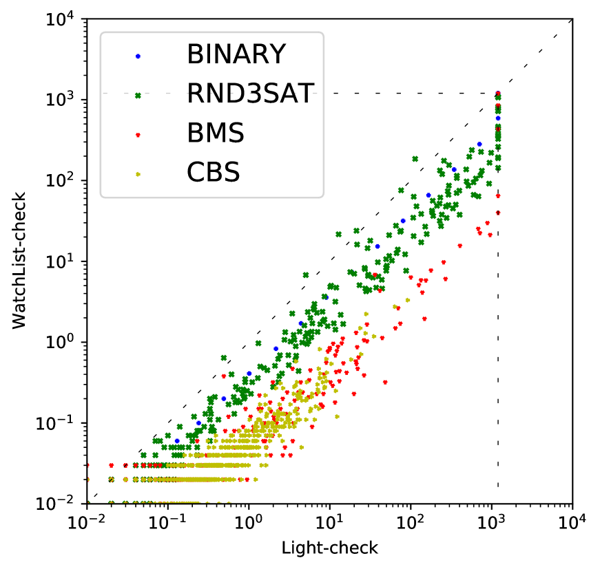
(a) CPU Time (in seconds)

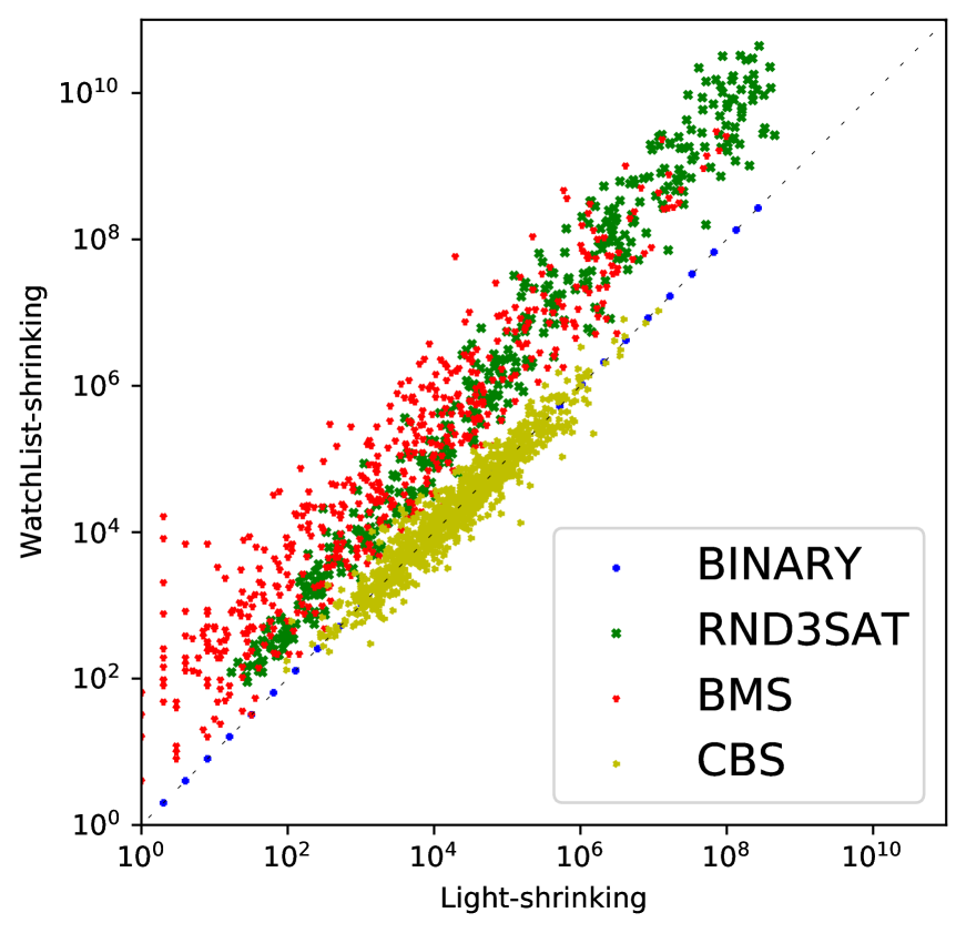
(b) # of partial models

Figure 1: Scatter plot comparing CPU time and log-total # of partial models with the two implicant shrinking algorithms.

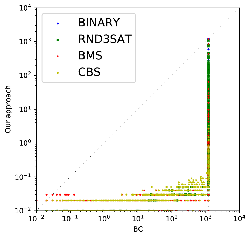
(a) BC

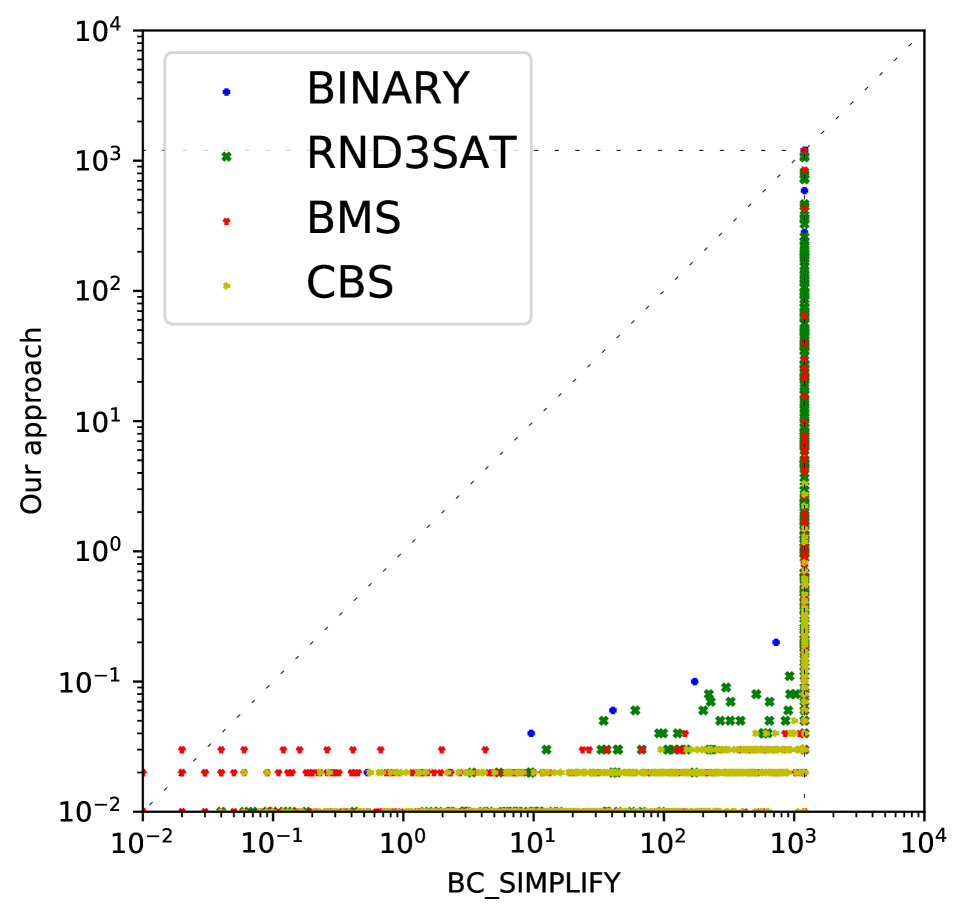
(b) BC_Partial

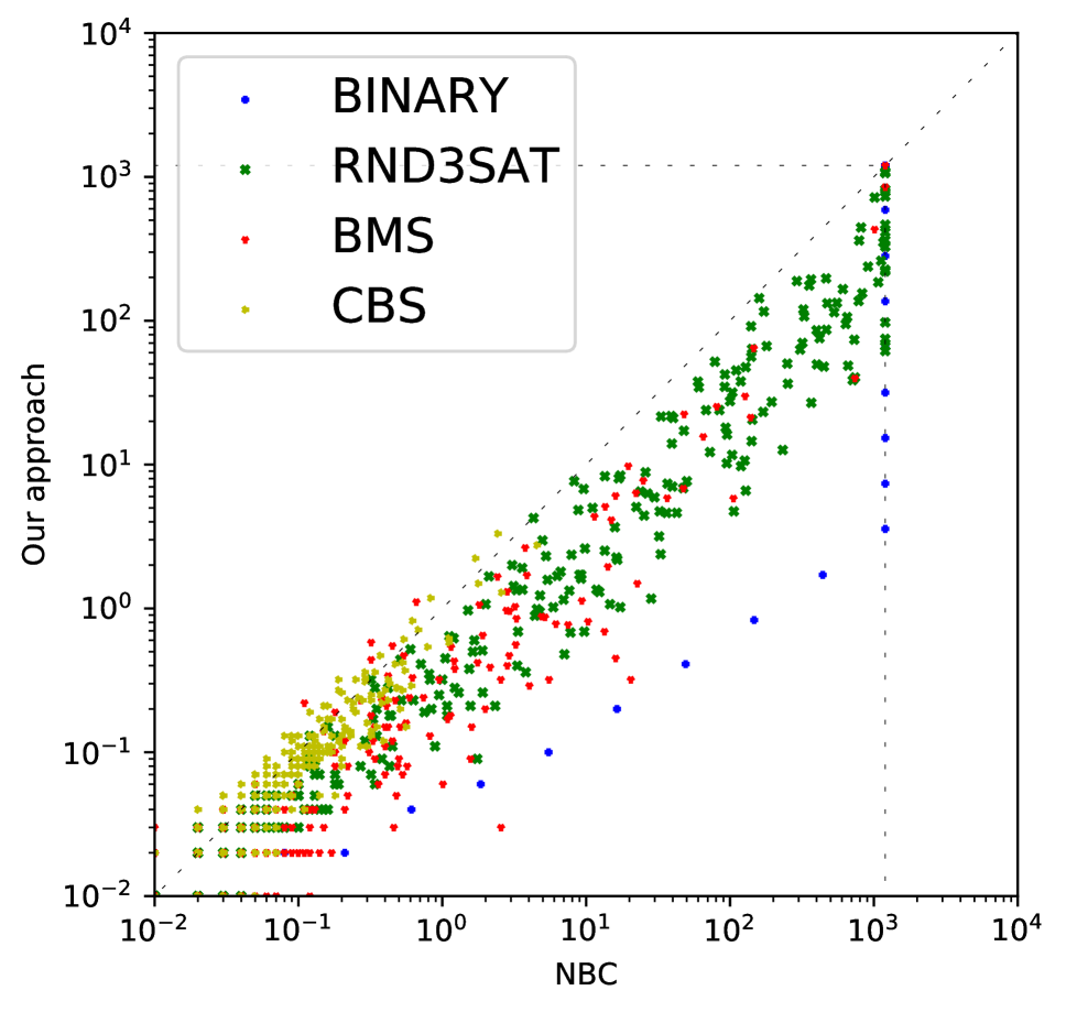
(c) NBC

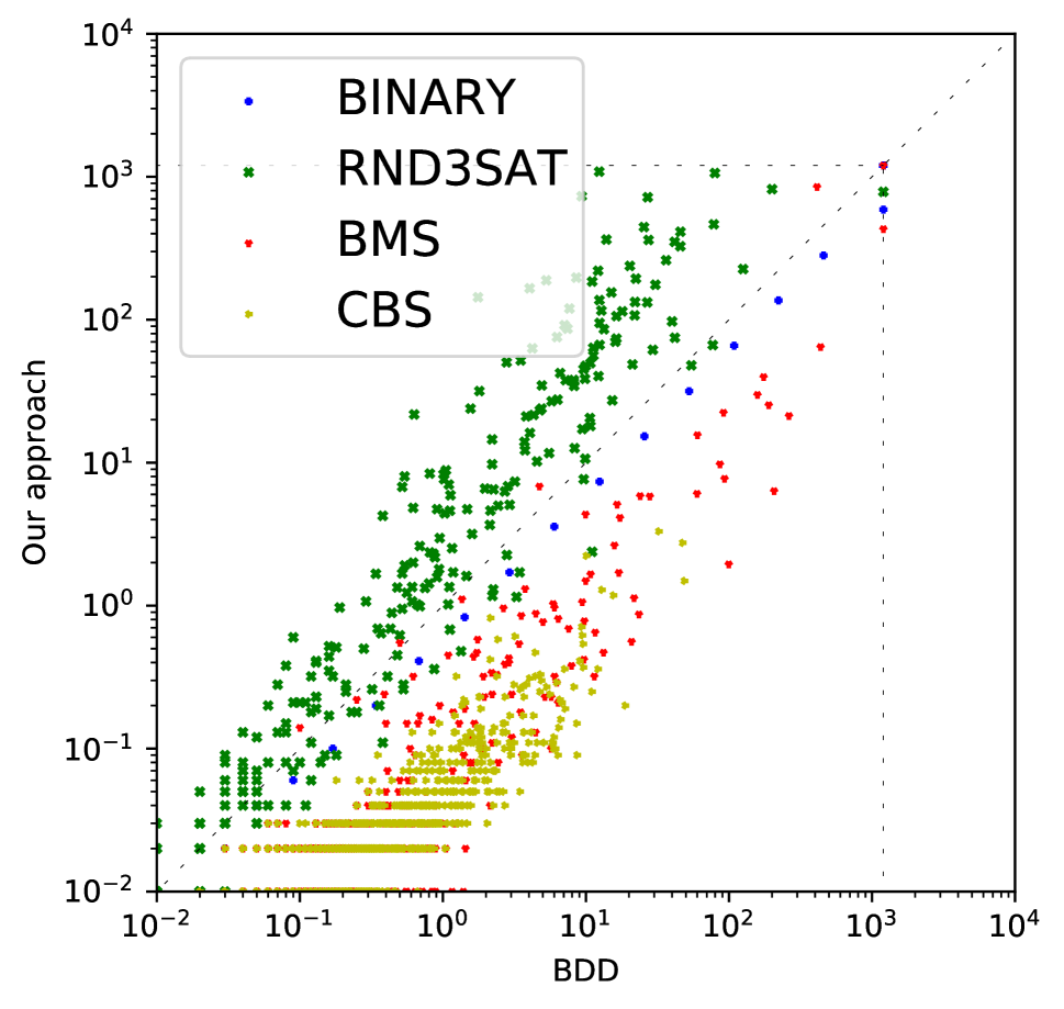
(d) BDD

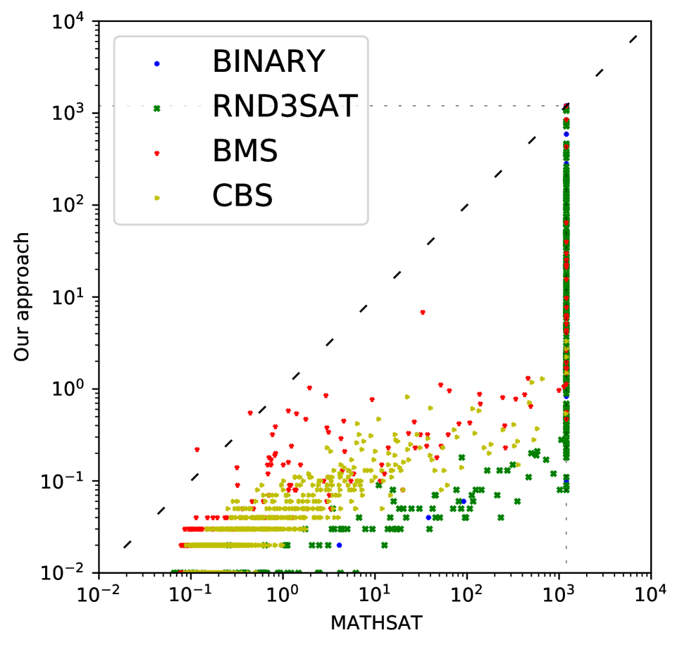
(e) MathSAT

Figure 2: Scatter plots comparing TabularAllSAT CPU times against the other AllSAT solvers. The $x$ and $y$ axes are both log-scaled.

The benchmarks used on related works on enumeration (Toda and Soh 2016) are typically from SATLIB (Hoos and Stützle 2000), which were thought for SAT solving. However, most of these benchmarks are not suited for AllSAT solving: some benchmarks are UNSAT or admit only a couple of solutions, whereas others are encoded in a way that no total assignment can be shrunk into a partial one. For the sake of significance for AllSAT, we considered benchmarks having two characteristics: ($i$) each problem admits a high number of total assignments; ($ii$) the problem structure allows for some minimization of assignments, to test the efficiency of the chronological implicant shrinking algorithms.

Binary clauses is a crafted dataset containing problems with $n$ variables defined by binary clauses in the form:

$$(x_{1}\vee x_{n})\wedge(x_{2}\vee x_{n-1})\wedge...\wedge(x_{n/2-1}\vee x_{n/2})$$

Finding all solutions poses a significant challenge: retrieving all possible assignments requires returning $3^{n/2}$ assignments within a feasible timeframe.

Rnd3sat contains 410 random 3-SAT problems with $n$ variables, $n\in[10,50]$. In SAT instances, the ratio of clauses to variables needed to achieve maximum hardness is about 4.26, but in AllSAT, it should be set to approximately 1.5 (Bayardo Jr and Schrag 1997). For this reason, we choose not to use the instances uploaded to SATLIB and we created new random 3-SAT problems accordingly.

We also tested our algorithms over SATLIB benchmarks, specifically CBS and BMS (Singer, Gent, and Smaill 2000).

Comparing Implicant Shrinking Techniques

In Figure 1 we compare the two implicant shrinking algorithms with respect to CPU time and the number of disjoint partial assignments. We checked the correctness of the enumeration by testing if the number of total assignments covered by the set of partial solutions was the same as the model count reported by the #SAT solver Ganak (Sharma et al. 2019), being always correct for both algorithms.

Results suggest that, with no surprise, dynamically updating watches is more effective in shrinking total assignments. When considering time efficiency, however, the faster but conservative simplification algorithm outperforms the other variant. The computational cost of updating each watch list $\omega(\ell)$ significantly slows down the computation process the higher the number of total models satisfying $F$ is.

All the experiments in the following subsections assume TabularAllSAT relies on the lighter variant.

Baseline Solvers

We considered BC, NBC, and BDD (Toda and Soh 2016), respectively a blocking, a non-blocking, and a BDD-based disjoint AllSAT solver. BC also provides the option to obtain partial assignments (from now on BC_Partial). Lastly, we considered MathSAT5 (Cimatti et al. 2013), since it provides an interface to compute partial enumeration of propositional problems by exploiting blocking clauses.

Some other AllSAT solvers, such as BASolver (Zhang, Pu, and Sun 2020) and AllSATCC (Liang et al. 2022), are currently not publicly available, as reported also in another paper (Fried, Nadel, and Shalmon 2023).

Results

Table 1 reports the number of instances solved by each solver for each set of benchmarks before reaching timeout, where ”solved” means that they enumerated completely a set of disjoint partial models covering all total models. We see that TabularAllSAT solves the highest amount of instances for each benchmark, even though BDD and NBC are close. We also present some scatter plots comparing TabularAllSAT time performance against each of the other AllSAT solvers available, using different marks and colors to distinguish instances from different benchmarks. The CPU times reported in Figure 2 consider only the time taken to reach each assignment, without storing them.

TabularAllSAT outperforms all the other solvers in every benchmark excluding rnd3sat, where BDD outperforms our approach. The latter instances are not structurally complex due to the low clause-to-variable ratio and can be compiled into BDDs with minimal inefficiencies, thus justifying this behavior: the higher the number of clauses is, the more challenging the compilation of the propositional formula into a BDD is, as we can see with BMS and CSB.

Conclusion

We presented an AllSAT procedure that combines CDCL, CB, and chronological implicant shrinking to perform partial disjoint enumeration. The experiments confirm the benefits of combining them, avoiding both performance degradations due to blocking clauses and bottlenecks generated by the solver being stuck in non-satisfiable search sub-trees.

This work could be extended in several directions. First, we plan to compare our algorithm against other enumeration algorithms based on knowledge compilation (for instance D4 (Lagniez and Marquis 2017)), even though this might involve a potentially costly compilation process before enumeration and accordingly such an approach is not any-time. Then, to further improve the performances of TabularAllSAT, we plan to explore novel decision heuristics that are suitable for chronological backtracking. Finally, we plan to extend our techniques to handle also projected enumeration and to investigate the integration of chronological backtracking with component caching.

References

- Bayardo Jr and Pehoushek (2000) Bayardo Jr, R. J.; and Pehoushek, J. D. 2000. Counting models using connected components. In AAAI/IAAI, 157–162.
- Bayardo Jr and Schrag (1997) Bayardo Jr, R. J.; and Schrag, R. 1997. Using CSP look-back techniques to solve real-world SAT instances. In Aaai/iaai, 203–208. Citeseer.
- Chistikov, Dimitrova, and Majumdar (2015) Chistikov, D.; Dimitrova, R.; and Majumdar, R. 2015. Approximate counting in SMT and value estimation for probabilistic programs. In Tools and Algorithms for the Construction and Analysis of Systems: 21st International Conference, TACAS 2015, Held as Part of the European Joint Conferences on Theory and Practice of Software, ETAPS 2015, London, UK, April 11-18, 2015, Proceedings 21, 320–334. Springer.
- Cimatti et al. (2013) Cimatti, A.; Griggio, A.; Schaafsma, B. J.; and Sebastiani, R. 2013. The MathSAT5 SMT solver. In Tools and Algorithms for the Construction and Analysis of Systems: 19th International Conference, TACAS 2013, Held as Part of the European Joint Conferences on Theory and Practice of Software, ETAPS 2013, Rome, Italy, March 16-24, 2013. Proceedings 19, 93–107. Springer.
- Davis, Logemann, and Loveland (1962) Davis, M.; Logemann, G.; and Loveland, D. 1962. A machine program for theorem-proving. Communications of the ACM, 5(7): 394–397.
- Déharbe et al. (2013) Déharbe, D.; Fontaine, P.; Le Berre, D.; and Mazure, B. 2013. Computing prime implicants. In 2013 Formal Methods in Computer-Aided Design, 46–52. IEEE.
- Dlala et al. (2016) Dlala, I. O.; Jabbour, S.; Sais, L.; and Yaghlane, B. B. 2016. A comparative study of SAT-based itemsets mining. In Research and Development in Intelligent Systems XXXIII: Incorporating Applications and Innovations in Intelligent Systems XXIV 33, 37–52. Springer.
- Fried, Nadel, and Shalmon (2023) Fried, D.; Nadel, A.; and Shalmon, Y. 2023. AllSAT for Combinational Circuits. In 26th International Conference on Theory and Applications of Satisfiability Testing (SAT 2023). Schloss Dagstuhl-Leibniz-Zentrum für Informatik.
- Grumberg, Schuster, and Yadgar (2004) Grumberg, O.; Schuster, A.; and Yadgar, A. 2004. Memory efficient all-solutions SAT solver and its application for reachability analysis. In Formal Methods in Computer-Aided Design: 5th International Conference, FMCAD 2004, Austin, Texas, USA, November 15-17, 2004. Proceedings 5, 275–289. Springer.
- Hoos and Stützle (2000) Hoos, H. H.; and Stützle, T. 2000. SATLIB: An online resource for research on SAT. Sat, 2000: 283–292.
- Huang and Darwiche (2005) Huang, J.; and Darwiche, A. 2005. Using DPLL for efficient OBDD construction. In Theory and Applications of Satisfiability Testing: 7th International Conference, SAT 2004, Vancouver, BC, Canada, May 10-13, 2004, Revised Selected Papers 7, 157–172. Springer.
- Jin, Han, and Somenzi (2005) Jin, H.; Han, H.; and Somenzi, F. 2005. Efficient conflict analysis for finding all satisfying assignments of a Boolean circuit. In Tools and Algorithms for the Construction and Analysis of Systems: 11th International Conference, TACAS 2005, Held as Part of the Joint European Conferences on Theory and Practice of Software, ETAPS 2005, Edinburgh, UK, April 4-8, 2005. Proceedings 11, 287–300. Springer.
- Khurshid et al. (2004) Khurshid, S.; Marinov, D.; Shlyakhter, I.; and Jackson, D. 2004. A case for efficient solution enumeration. In Theory and Applications of Satisfiability Testing: 6th International Conference, SAT 2003, Santa Margherita Ligure, Italy, May 5-8, 2003, Selected Revised Papers 6, 272–286. Springer.
- Lagniez and Marquis (2017) Lagniez, J.-M.; and Marquis, P. 2017. An Improved Decision-DNNF Compiler. In IJCAI, volume 17, 667–673.
- Lahiri, Bryant, and Cook (2003) Lahiri, S. K.; Bryant, R. E.; and Cook, B. 2003. A symbolic approach to predicate abstraction. In Computer Aided Verification: 15th International Conference, CAV 2003, Boulder, CO, USA, July 8-12, 2003. Proceedings 15, 141–153. Springer.
- Li, Hsiao, and Sheng (2004) Li, B.; Hsiao, M. S.; and Sheng, S. 2004. A novel SAT all-solutions solver for efficient preimage computation. In Proceedings Design, Automation and Test in Europe Conference and Exhibition, volume 1, 272–277. IEEE.
- Liang et al. (2022) Liang, J.; Ma, F.; Zhou, J.; and Yin, M. 2022. AllSATCC: Boosting AllSAT Solving with Efficient Component Analysis. In IJCAI, 1866–1872.
- Marques-Silva and Sakallah (1999) Marques-Silva, J. P.; and Sakallah, K. A. 1999. GRASP: A search algorithm for propositional satisfiability. IEEE Transactions on Computers, 48(5): 506–521.
- McMillan (2002) McMillan, K. L. 2002. Applying SAT methods in unbounded symbolic model checking. In Computer Aided Verification: 14th International Conference, CAV 2002 Copenhagen, Denmark, July 27–31, 2002 Proceedings 14, 250–264. Springer.
- Möhle and Biere (2019a) Möhle, S.; and Biere, A. 2019a. Backing backtracking. In Theory and Applications of Satisfiability Testing–SAT 2019: 22nd International Conference, SAT 2019, Lisbon, Portugal, July 9–12, 2019, Proceedings 22, 250–266. Springer.
- Möhle and Biere (2019b) Möhle, S.; and Biere, A. 2019b. Combining Conflict-Driven Clause Learning and Chronological Backtracking for Propositional Model Counting. In GCAI, 113–126.
- Möhle, Sebastiani, and Biere (2020) Möhle, S.; Sebastiani, R.; and Biere, A. 2020. Four flavors of entailment. In International Conference on Theory and Applications of Satisfiability Testing, 62–71. Springer.
- Möhle, Sebastiani, and Biere (2021) Möhle, S.; Sebastiani, R.; and Biere, A. 2021. On Enumerating Short Projected Models. arXiv preprint arXiv:2110.12924.
- Morettin, Passerini, and Sebastiani (2019) Morettin, P.; Passerini, A.; and Sebastiani, R. 2019. Advanced SMT techniques for weighted model integration. Artificial Intelligence, 275: 1–27.
- Morgado and Marques-Silva (2005a) Morgado, A.; and Marques-Silva, J. 2005a. Good learning and implicit model enumeration. In 17th IEEE International Conference on Tools with Artificial Intelligence (ICTAI’05), 6 pp.–136.
- Morgado and Marques-Silva (2005b) Morgado, A.; and Marques-Silva, J. 2005b. Good learning and implicit model enumeration. In 17th IEEE International Conference on Tools with Artificial Intelligence (ICTAI’05), 6–pp. IEEE.
- Moskewicz et al. (2001) Moskewicz, M. W.; Madigan, C. F.; Zhao, Y.; Zhang, L.; and Malik, S. 2001. Chaff: Engineering an efficient SAT solver. In Proceedings of the 38th annual Design Automation Conference, 530–535.
- Nadel and Ryvchin (2018) Nadel, A.; and Ryvchin, V. 2018. Chronological backtracking. In Theory and Applications of Satisfiability Testing–SAT 2018: 21st International Conference, SAT 2018, Held as Part of the Federated Logic Conference, FloC 2018, Oxford, UK, July 9–12, 2018, Proceedings 21, 111–121. Springer.
- Sebastiani (2020) Sebastiani, R. 2020. Are You Satisfied by This Partial Assignment? arXiv preprint arXiv:2003.04225.
- Sharma et al. (2019) Sharma, S.; Roy, S.; Soos, M.; and Meel, K. S. 2019. GANAK: A Scalable Probabilistic Exact Model Counter. In Proceedings of International Joint Conference on Artificial Intelligence (IJCAI).
- Singer, Gent, and Smaill (2000) Singer, J.; Gent, I. P.; and Smaill, A. 2000. Backbone fragility and the local search cost peak. Journal of Artificial Intelligence Research, 12: 235–270.
- Spallitta et al. (2022) Spallitta, G.; Masina, G.; Morettin, P.; Passerini, A.; and Sebastiani, R. 2022. SMT-based weighted model integration with structure awareness. In Uncertainty in Artificial Intelligence, 1876–1885. PMLR.
- Toda and Soh (2016) Toda, T.; and Soh, T. 2016. Implementing efficient all solutions SAT solvers. Journal of Experimental Algorithmics (JEA), 21: 1–44.
- Yu et al. (2014) Yu, Y.; Subramanyan, P.; Tsiskaridze, N.; and Malik, S. 2014. All-SAT using minimal blocking clauses. In 2014 27th International Conference on VLSI Design and 2014 13th International Conference on Embedded Systems, 86–91. IEEE.
- Zhang, Pu, and Sun (2020) Zhang, Y.; Pu, G.; and Sun, J. 2020. Accelerating All-SAT computation with short blocking clauses. In Proceedings of the 35th IEEE/ACM International Conference on Automated Software Engineering, 6–17.