The Mini-batch Stochastic Conjugate Algorithms with the unbiasedness and Minimized Variance Reduction

Abstract

We firstly propose the new stochastic gradient estimate of unbiasedness and minimized variance in this paper. Secondly, we propose the two algorithms: Algorithm1 and Algorithm2 which apply the new stochastic gradient estimate to modern stochastic conjugate gradient algorithms SCGA kou2022mini and CGVR jin2018stochastic . Then we prove that the proposed algorithms can obtain linear convergence rate under assumptions of strong convexity and smoothness. Finally, numerical experiments show that the new stochastic gradient estimate can reduce variance of stochastic gradient effectively. And our algorithms compared with SCGA and CGVR can convergent faster in numerical experiments on ridge regression model.

1 Introduction

With the development of big data, machine learning and deep learning is widely used in various fields. Many machine learning and deep learning problems can be described by the following finite-sum minimization problem.

$$\min\limits_{\omega\in R^{d}}f(\omega)=\frac{1}{n}\sum_{i=1}^{n}f_{i}(\omega)$$ (1)

Here $\omega$ is the decision variable, $f_{i}(\omega):R^{d}\to R$ is the loss function of $i$-th sample. When sample size $n$ is very large, it takes a lot of time calculating the gradient of the objective function to solve (1). Therefore, in order to reduce computation cost, a natural idea is that the full gradient at each iteration is replaced by calculating gradient of a random sample or average gradient over a mini-batch of random sample.

The earliest algorithm using this idea is stochastic gradient descent algorithm (SGD) bottou2010large . SGD and its variants dozat2016incorporating reddi2019convergence is widely used to minimize the loss function in large-scale machine learning problems for its advantages of the low computation cost. However, due to the variance of stochastic gradient, SGD can only reach an approximate solution if fixed step sizes are used, or it only obtains a slower sub-linear convergence rate if decreasing step sizes are used. In order to improve the convergence rate of SGD, many researchers design methods which can reduce the variance of stochastic gradient using historical information or periodically calculated full gradient information, such as SAG schmidt2017minimizing , SAGA defazio2014saga , SVRG johnson2013accelerating et al.

The stochastic gradient with variance reduction used in SVRG and SAGA algorithms is an unbiased estimate of the full gradient, but its variance is larger than SAG which is biased. A desired gradient estimate should be unbiased and has small variance. So we propose the new stochastic gradient estimate with unbiasedness and minimal vriance named. Based on our research interests, we mainly focus on applying the new stochastic gradient estimate in stochastic conjugate gradient methods.

Conjugate gradient methods is one class of the main methods for solving large-scale optimization problems. They have different formulas of $\beta_{k}$ among various conjugate gradient methods. The best-known standard formulas for $\beta_{k}$ are called the Fletcher–Reeves (FR) fletcher1964function , Polak–Ribière–Polyak (PRP) polak1969note polyak1969conjugate , Hestenes–Stiefel (HS) hestenes1952methods , Liu–Storey (LS) liu1991efficient and Dai-Yuan (DY) dai1999nonlinear formulas. Moreover, there is a large variety of hybrid conjugate gradient methods, such as TAS touati1990efficient , PRP-FR hu1991global , GN gilbert1992global et al. The hybrid conjugate gradient methods combine the properties of the standard ones in order to get new ones, rapid convergent to the solution andrei2020nonlinear . By mining the second-order information and analyzing the relationship between the conjugate direction and the quasi-Newton direction, proposed conjugate gradient methods includes: Dai and Kou dai2013nonlinear and Hager and Zhang hager2005new hager2013limited . More details about conjugate gradients can be found in andrei2020nonlinear Dai2020nonlinear . Recently, CGVR jin2018stochastic and SCGA kou2022mini which is two kinds of stochastic conjugate gradient algorithms with variance reduction is proposed. The researchers find that stochastic conjugate gradient method can reach the convergence point faster than stochastic gradient descent algorithms. so we propose the two improved stochastic conjugate gradient algorithms which apply the new stochastic gradient estimate mentioned above in SCGA kou2022mini and CGVR algorithms jin2018stochastic .

The rest of this paper organize is as follows: Section 2 proposes the new stochastic gradient estimate with the unbiasedness and minimized variance. Section 3 describes the details of Algorithm1 and Algorithm2. The convergence of our algorithms are proved in Section 4. In the end, Section 5 shows the results of our numerical experiments and Section 6 concludes this paper.

2 A New Stochastic Gradient Estimate with Unbiasedness and Minimized Variance (SGMV)

Firstly, let’s review the characteristics of stochastic gradient estimate with variance reduction in the literature. The stochastic gradient estimates of SAGA and SVRG is simplified to

$$g_{k}=\nabla f_{S_{k}}(\omega_{k})-\nabla f_{S_{k}}(\phi_{k})+\frac{1}{n}\sum_{i=1}^{n}\nabla f_{i}(\phi_{i}^{k})$$ (2)

where there is a high correlation between $\nabla f_{S_{k}}(\omega_{k})$ and $\nabla f_{S_{k}}(\phi_{k})$. The selection of $\phi_{k}$ in SVRG and SAGA is different. Based on $\nabla f_{S_{k}}(\omega_{k})$, $g_{k}$ includes the difference between the stochastic gradient of mini-batch sample $S_{k}$ and full gradient, so it can correct $\nabla f_{S_{k}}(\omega_{k})$ and make it closer to the full gradient $\frac{1}{n}\sum_{i=1}^{n}\nabla f_{i}(\omega_{i}^{k})$.

For the convenience of analysis, we define that

$$X_{j}=\nabla f_{j}(\omega_{k}),Y_{j}=\nabla f_{j}(\phi_{k})$$ (3)

$$\bar{X}=\nabla f_{S_{k}}(\omega_{k}),\bar{Y}=\nabla f_{S_{k}}(\phi_{k}),E(\bar{Y})=\frac{1}{n}\sum_{i=1}^{n}\nabla f_{i}(\phi_{i}^{k})$$ (4)

where $X_{j}$ and $Y_{j}$ are respectively the stochastic gradient of sample $j$ at iteration point $\omega_{k}$ and $\phi_{k}$, $\bar{X}$ and $\bar{Y}$ is the mean of $X_{j}$ and $Y_{j}$, $j\in S_{k}$. In order to find unbiased stochastic gradient estimate, we define the general form of stochastic gradient estimate

$$\theta_{\gamma}=\bar{X}-\gamma(\bar{Y}-E(\bar{Y}))$$

Specifically, the $\theta_{\gamma=1}$ is stochastic gradient estimate (2). Next, through the following analysis of the expectation and variance of $\theta_{\gamma}$, a better stochastic gradient estimate $\gamma^{*}$ which minimize the variance of $\theta_{\gamma}$ is found in this general form.

Firstly, $\theta_{\gamma}$ is an unbiased estimate to $E(\bar{X})$ .i.e.

$$E(\theta_{\gamma})=E(\bar{X})=\nabla f(\omega_{k})$$ (5)

And the variance of $\theta_{\gamma}$ is

$$Var(\theta_{\gamma}) =Var(\bar{X}-\gamma(\bar{Y}-E(\bar{Y})))$$ (6)

$$=Var(\bar{X})+Var(\gamma(\bar{Y}-E(\bar{Y})))-2Cov(\bar{X},\gamma(\bar{Y}-E(\bar{Y})))$$

$$=Var(\bar{X})+\gamma^{2}Var(\bar{Y})-2\gamma Cov(\bar{X},\bar{Y})$$

$Var(\theta_{\gamma})$ is a quadratic function about $\gamma$ , so we can easily obtain its minimizer

$$\gamma^{*}=\frac{Cov(\bar{X},\bar{Y})}{Var(\bar{Y})}$$ (7)

When $\gamma$ is taken to $\gamma^{*}$,

$$Var(\theta_{\gamma=\gamma^{*}})=Var(\bar{X})(1-\rho_{\bar{X}\bar{Y}}^{2})$$ (8)

where $\rho_{\bar{X}\bar{Y}}$ is correlation coefficient of random variable $\bar{X}$ and $\bar{Y}$. Because $\rho_{\bar{X}\bar{Y}}\in[-1,1]$ yields $Var(\theta_{\gamma=\gamma^{*}})\leq Var(\bar{X})$, so $\theta_{\gamma=\gamma^{*}}$ is a stochastic gradient estimate of variance reduction. In addition, as iteration number $k$ increases and $\rho_{\bar{X}\bar{Y}}$ increases, then $Var(\theta_{\gamma=\gamma^{*}})$ decreases. In particular, if $\omega_{k}$ is near the optimal value $\omega^{*}$, $\rho_{\bar{X}\bar{Y}}\rightarrow 1$, $Var(\theta_{\gamma=\gamma^{*}})\rightarrow 0$. In a word, iterating around the optimal value, $\theta_{\gamma=\gamma^{*}}$ is less affected by variance. Furthermore, due to $Var(\theta_{\gamma=\gamma^{*}})\leq Var(\theta_{\gamma=1})$, we see easily that $\theta_{\gamma=\gamma^{*}}$ is the better stochastic gradient estimate than $\theta_{\gamma=1}$ in SAGA/SVRG.

In order to calculate $\gamma^{*}$, we need to estimate $Cov(\bar{X},\bar{Y})$ and $Var(\bar{Y})$ with known sample data. We mainly use the basic statistic theory about survey sampling to estimate them. We assume that mini-batch sample $S_{k}$ is sampled with replacement and each mini-batch sample is of size $|S|$. it is easy to obtain that

$$Cov(\bar{X},\bar{Y}) =Cov(\frac{1}{|S|}\sum_{j\in S_{k}}X_{j},\frac{1}{|S|}\sum_{j\in S_{k}}Y_{j})$$ (9)

$$=\frac{1}{|S|^{2}}Cov(\sum_{j\in S_{k}}X_{j},\sum_{j\in S_{k}}Y_{j})$$

$$=\frac{1}{|S|^{2}}\sum_{j\in S_{k}}Cov(X_{j},Y_{j})$$

$$\approx\frac{1}{|S|}s_{XY}$$

$$Var(\bar{Y}) =Var(\frac{1}{|S|}\sum_{j\in S_{k}}Y_{j})$$ (10)

$$=\frac{1}{|S|^{2}}Var(\sum_{j\in S_{k}}Y_{j})$$

$$=\frac{1}{|S|^{2}}\sum_{j\in S_{k}}Var(Y_{j})$$

$$\approx\frac{1}{|S|}s_{Y}^{2}$$

(LABEL:2:cov_estimate) and (LABEL:2:var_estimate) show the process of $Cov(\bar{X},\bar{Y})$ and $Var(\bar{Y})$ estimated. Inside, the variance and covariance calculations are the elementwise operation. The estimation process of $Cov(\bar{X},\bar{Y})$ is described as follows: the first equality use the definition of $\bar{X}$ and $\bar{Y}$.Then by using the properties of covariance, it yields the second equality. $X_{i}$ and $X_{j}$ ($i\neq j$) are independent that yield $Cov(X_{i},X_{j})=0$, so the third equality hold. Finally,in fourth equality the covariance $Cov(X_{j},Y_{j})$ is estimated by the sample covariance $s_{XY}$ approximatively. Similarly, $Var(\bar{Y})$ is estimated by the sample variance $s_{XY}$. Note that $s_{XY}$ and $s_{Y}^{2}$ is defined as (11).

$$s_{XY} =\frac{1}{|S|-1}\sum_{j\in S_{k}}(X_{j}-\bar{X})(Y_{j}-\bar{Y})$$ (11)

$$s_{Y}^{2} =\frac{1}{|S|-1}\sum_{j\in S_{k}}(Y_{j}-\bar{Y})^{2}$$

To sum up, $\gamma^{*}$ can be estimated by ratio of $s_{XY}$ and $s_{Y}^{2}$

$$\gamma^{*}=\frac{Cov(\bar{X},\bar{Y})}{Var(\bar{Y})}\approx\frac{s_{XY}}{s_{Y}^{2}}$$ (12)

Based on the above analysis, the new stochastic gradient estimate $\theta_{\gamma=\gamma^{*}}$ with unbiasedness and minimal variance is as follows:

$$g_{k} =\nabla f_{S_{k}}(\omega^{k})-\gamma^{*}(\nabla f_{S_{k}}(\phi_{k})-\frac{1}{n}\sum_{i=1}^{n}\nabla f_{i}(\phi_{i}^{k}))$$ (13)

$$\text{where }\gamma^{*} \approx\frac{s_{XY}}{s_{Y}^{2}}$$

The new estimate can generate many algorithms based on $\phi_{k}$ which can be flexibly designed. The stronger the correlation between $\nabla f_{S_{k}}(\omega^{k})$ and $\nabla f_{S_{k}}(\phi_{k})$, the better the effect of the new stochastic gradient estimate.

Compared with $\gamma=1$, vector $\gamma=\gamma^{*}$ can be adjusted by each component of gradient and information of every iterations. Therefore, the new stochastic gradient estimate has adaptive parameter.

3 Algorithm

Appling the new stochastic gradient estimate to SCGA and CGVR, we propose the improvement algorithms of SCGA and CGVR. In this section, we describe the details of two new algorithms.

3.1 SCGA with the minimal variance stochastic gradient estimate

The main framework of Algorithm1 is as follows:

1 Initialization: Given $\omega_{0}\in R^{d}$, compute the full gradient matix at initial iterate $\omega_{0}$ and store it:

2 for $i=1,2...n$ do

3      Compute $\nabla f_{i}(\omega_{0})$

4       Store $\nabla f(\omega_{[0]})\leftarrow\nabla f_{i}(\omega_{0})$

5$\mu_{0}=\frac{1}{n}\sum_{i=1}^{n}\nabla f_{i}(\omega_{[0]})$

6 Set the initial stochastic gradient $g_{0}=\mu_{0}.$

7 Set the initial direction $d_{0}=-g_{0}$

8 Iteration:

9 for $k=1,2...$ do

10       Compute the stepsize $\alpha_{k-1}$ satisfying (14) and (15)

11       Update $\omega_{k}=\omega_{k-1}+\alpha_{k-1}d_{k-1}$

12       Randomly sample a mini-batch sample $S_{k}$

13       for $j:S_{k}$ do

14             Compute $\nabla f_{j}(\omega_{k})$ and store it into matrix $\nabla f_{[S_{k}]}(\omega_{k})$

15             Select $\nabla f_{j}(\omega_{[k-1]})$ in $\nabla f(\omega_{[k-1]})$ and store it into matrix $\nabla f_{[S_{k}]}(\omega_{[k-1]})$

16            

17      for $r=1,2...d$ do

18             Using (11), compute the sample covariance of $\nabla f_{[S_{k}]}^{(r)}(\omega_{k})$ and $\nabla f_{[S_{k}]}^{(r)}(\omega_{[k-1]})$, the sample variance of $\nabla f_{[S_{k}]}^{(r)}(\omega_{[k-1]})$

19             Using (13) Compute $\gamma^{*(r)}$

20      Compute $\nabla f_{S_{k}}(\omega_{k})=\frac{1}{|S|}\sum_{j\in S_{k}}\nabla f_{j}(\omega_{k}),\mu_{S_{k}}=\frac{1}{|S|}\sum_{j\in S_{k}}\nabla f_{j}(\omega_{[k-1]})$

21       Compute $g_{k}=\nabla f_{S_{k}}(\omega_{k})-\gamma^{*}(\mu_{S_{k}}-\mu_{k-1})$

22       Compute $\beta_{k}=\beta_{k}^{PRP-FR},\beta_{k}^{PRP-FR}$ using (16)

23       Update $d_{k}=-g_{k}+\beta_{k}d_{k-1}$

24       Update $\nabla f(\omega_{[k]})$ using (18)

25       Update $\mu_{k}=\frac{1}{n}\sum_{j=1}^{n}\nabla f_{j}(\omega_{[k]})$

Algorithm 1 SCGA with the minimal variance stochastic gradient estimate

Algorithm1 is mainly divided into two parts: initialization and iteration. In initialization, we compute gradient $\nabla f_{i}(\omega_{[0]})$ of each samples $i$ at the initial iteration point $\omega_{0}$ and store in the matrix

$$\nabla f(\omega_{[0]})=(\nabla f_{1}(\omega_{[0]}),\nabla f_{2}(\omega_{[0]}),...,\nabla f_{n}(\omega_{[0]}))$$

Then, we compute the full gradient $\mu_{0}$ at $\omega_{0}$, set initial stochastic gradient $g_{0}=\mu_{0}$ and initial direction $d_{0}=-g_{0}$ to compute the first iteration point $\omega_{1}$.
In iteration, the step size $\alpha_{k-1}$ satisfies the following strong Wolfe conditions:

$$f_{S_{k}}(\omega_{k}+\alpha_{k}d_{k})\leq f_{S_{k}}(\omega_{k})+\sigma_{1}\alpha_{k}g_{k}^{T}d_{k}$$ (14)

$$|g_{k+1}^{T}d_{k}|\leq-\sigma_{2}g_{k}^{T}d_{k}$$ (15)

where $0<\sigma_{1}<\sigma_{2}<1$. Then, it is easy to obtain the next iteration point $\omega_{k}=\omega_{k-1}+\alpha_{k-1}d_{k-1}$. Next, we determine the next search direction. The search direction $d_{k}$ is updated by $d_{k}=-g_{k}+\beta_{k}d_{k-1}$. For the choice of $\beta_{k}$ , our algorithm uses $\beta_{k}^{PRP-FR}$hu1991global which performs better than other hyhid conjugate gradient algorithmsandrei2020nonlinear such as $\beta_{k}^{TAS}$touati1990efficient and $\beta_{k}^{GN}$gilbert1992global . $\beta_{k}^{PRP-FR}$hu1991global . It combines the properties of $\beta^{PRP}$ and $\beta^{FR}$ in order to be convergent rapidly. And the upperbound of $|\beta_{k}^{PRP-FR}|$ is $\beta_{k}^{FR}$ so that the proof of convergence in section 4 holds. $\beta_{k}^{PRP-FR}$ is implemented as

$$\beta_{k}^{PRP-FR}=max\{0,min\{\beta^{PRP},\beta^{FR}\}\}$$ (16)

where

$$\beta_{k}^{PRP}=\frac{g_{k}^{T}(g_{k}-g_{k-1})}{\|g_{k-1}\|^{2}},\beta_{k}^{FR}=\frac{\|g_{k}\|^{2}}{\|g_{k-1}\|^{2}}$$ (17)

For the computation of stochastic gradient, our algorithm use the new stochastic gradient estimate which is proposed in Section 2. In the end of each iteration, we update the gradient matrix with that

$$\begin{split}\nabla f(\omega_{[k]})=\left\{\begin{array}[]{ll}\nabla f_{j}(\omega_{k}),&\forall j\in S_{k}\\ \nabla f_{j}(\omega_{[k-1]}),&\forall j\notin S_{k}\\ \end{array}\right.\end{split}$$ (18)

and compute the full gradient $\mu_{k}$ at $k$-th iteration.

3.2 CGVR with the minimal variance stochastic gradient estimate

The main framework of Algorithm2 is as follows:

1 Initialization: Given $x_{0}\in R^{d}$, compute $h_{0}=\frac{1}{n}\sum_{i=1}^{n}\nabla f_{i}(x_{0})$:

2 Iteration:

3 for $l=1,2...T$ do

4       $\mu_{l-1}=\frac{1}{n}\sum_{i=1}^{n}\nabla f_{i}(x_{l-1})$

5       Update $\omega_{0}=x_{l-1},g_{0}=h_{l-1},d_{0}=-g_{0}$

6       for $k=1,2...m$ do

7             Compute the stepsize $\alpha_{k-1}$ satisfying (14) and (15)

8             Update $\omega_{k}=\omega_{k-1}+\alpha_{k}d_{k-1}$

9             Randomly sampling a mini-batch sample $S_{k}$

10             for $j:S_{k}$ do

11                   Compute $\nabla f_{j}(\omega_{k}),\nabla f_{j}(\omega_{0})$

12                   Store $\nabla f_{[S_{k}]}(\omega_{k})\leftarrow\nabla f_{j}(\omega_{k}),\nabla f_{[S_{k}]}(\omega_{0})\leftarrow\nabla f_{j}(\omega_{0})$

13                  

14            for $r=1,2...d$ do

15                   Using (11), compute the sample covariance $\nabla f_{[S_{k}]}^{(r)}(\omega_{k})$ and $\nabla f_{[S_{k}]}^{(r)}(\omega_{0})$, the sample variance of $\nabla f_{[S_{k}]}^{(r)}(\omega_{0})$

16                   Compute $\gamma^{*(r)}$ using (13)

17            Compute $\nabla f_{S_{k}}(\omega_{k}),\nabla f_{S_{k}}(\omega_{0})$

18             Compute $g_{k}=\nabla f_{S_{k}}(\omega_{k})-\gamma^{*}(\nabla f_{S_{k}}(\omega_{0})-\mu_{l-1})$

19             Compute $\beta_{k}=\beta_{k}^{PRP-FR},\beta_{k}^{PRP-FR}$ using (16)

20             Update $d_{k}=-g_{k}+\beta_{k}d_{k-1}$

21            

22      Update $h_{l}=g_{m}$

23       Option I:$x_{l}=\omega_{m}$

24       Option II:$x_{l}=\omega_{k}$ for randomly chosen $k\in\{1,2...,m\}$

25      

Algorithm 2 CGVR with the minimal variance stochastic gradient estimate

The iteration of Algorithm2 is composed of inner loop and outer loop. The outer loop periodically updates the full gradient of iteration point $x_{l-1}$. In the inner loop iteration, according to the iteration direction $d_{k-1}$ of the previous step, we firstly get the new step size $\alpha_{k}$ with the inexact line search satisfying the strong Wolfe condition (14)(15). Second, we use stochastic conjugate gradient algorithm to determine the direction $d_{k}$ of the next iteration. Inside, Algorithm2 uses the new the stochastic gradient estimate, whereas CGVR uses the same stochastic gradient as SAGA. This is the main difference between Algorithm2 and CGVR. Due to the excellent characteristics of the new stochastic gradient estimate in variance reduction, Algorithm2 is a better stochastic conjugate gradient algorithm than CGVR.

Compared with Algorithm1,Algorithm2 has mainly the following differences. First, Algorithm2 needs to calculate full gradient for each outer loop, but does not need to store the gradient of each sample (see line 4 of the Algorithm2). Algorithm1 does not need to calculate the full gradient, but needs to use a large matrix to store the latest gradient of each sample (see line 2-4 of Algorithm1). So Algorithm2 has the characteristics of large computation and small storage, while Algorithm1 has the characteristics of low computation and large storage. Second, in the stochastic gradient estimate step of Algorithm2, the checkpoint is the initial point $w_{0}$ of the inner loop (see line 17 of Algorithm2), Algorithm1 use virtual checkpoint $\omega_{[k-1]}$ in stochastic gradient estimate(see line 20 of Algorithm1). Other details of Algorithm2 are similar to Algorithm1, so we don’t repeat them.

4 Convergence

Assumption 1($\mu$ -strong convexity and $L$ -smoothness) $f_{i},1\leq i\leq n$ is strongly convex and has Lipschitz continuous gradients, i.e.,

$$\mu I\prec\nabla^{2}f_{i}(w)\prec LI$$ (19)

For $\omega\in R^{d}$, $\mu$ is strong convexity constant and $L$ is Lipschitz constant.
Assumption 2 (lower and upper bounds of step size) Every step size $\alpha_{k}$ in Algorithm1 and Algorithm2 satisfies $\alpha_{1}\leq\alpha_{k}\leq\alpha_{2}$
Assumption 3 (upper bound of scalar $\beta_{k}$ ) There exists constant $\beta$ such that

$$\beta_{k}\leq\frac{\|g_{k}\|^{2}}{\|g_{k-1}\|^{2}}\leq\beta$$ (20)

Lemma 1

Under Assumption1, we have

$$2\mu(f(\omega)-f(\omega^{*}))\leq\|\nabla f(w)\|^{2}\leq 2L(f(\omega)-f(\omega^{*}))$$ (21)

Where $\omega\in R^{d}$, $\omega^{*}$ is the unique minimizer

Lemma 2

Consider that Algorithm1 and Algorithm2 (CG) algorithm, where step size $\alpha_{k}$ satisfies strong Wolfe condition with $0<\sigma_{2}<\frac{1}{2}$ and $\beta_{k}$ satisfies $|\beta_{k}|\leq\beta_{k}^{FR}$ , then it generates descent directions $d_{k}$ satisfying

$$-\frac{1}{1-\sigma_{2}}\leq\frac{\langle g_{k},d_{k}\rangle}{\|g_{k}\|^{2}}\leq\frac{2\sigma_{2}-1}{1-\sigma_{2}}$$ (22)

The proof of Lemma 2 is can be found in [17, lemma 3.1]. This lemma can give the lower and upper bound $\frac{\langle g_{k},d_{k}\rangle}{\|g_{k}\|^{2}}$, if the parameter $\beta_{k}$ is appropriately bounded in magnitude and $\alpha_{k}$ satisfies strong Wolfe conditions (14)(15). This conclusion is very important for the following proof of convergence. The following Theorem 1 and Theorem 2 show respectively the linear convergence of Algorithm1 and Algorithm2.

Theorem 4.1

Let Assumption 1,2,3 hold. If the bound of the step-size in Algorithm1 satisfies:

$$0<\alpha_{1}<\frac{1-\beta}{2L\sigma_{1}}$$ (23)

Then we have: $\forall k>0$

$$E(f(\omega_{k}))-f({\omega^{*}})\leq C\xi^{k}(E(f(\omega_{0}))-f(\omega^{*}))$$ (24)

where $\xi=\frac{(1-\sigma_{1})(1-\beta)+2L\alpha\sigma_{1}\sigma_{2}(1-\beta^{m})}{2\mu\sigma_{1}m(1-\sigma_{2})(1-\beta)}<1,\omega^{*}$ is the unique minimizer of $f$

Proof

It follows from strong Wolfe conditions (14) that

$$f_{S_{k}}(\omega_{k+1})-f_{S_{k}}(\omega_{k})\leq\sigma_{1}\alpha_{k}g_{k}^{T}d_{k}$$ (25)

Taking expectation on both sides of (25), we get

$$E(f(\omega_{k+1}))-f(\omega_{k})\leq\sigma_{1}E(\alpha_{k}g_{k}^{T}d_{k})$$ (26)

Then the definition of $d_{k}$ is used in (26), we have

$$E(f(\omega_{k+1}))-f(\omega_{k})\leq-\sigma_{1}E(\alpha_{k}\|g_{k}\|^{2})+\sigma_{1}E(\alpha_{k}\beta_{k}g_{k}^{T}d_{k-1})$$ (27)

Next, we apply Assumption 2 and strong Wolfe conditions (20) to get

$$E(f(\omega_{k+1}))-f(\omega_{k})\leq-\sigma_{1}\alpha_{1}E(\|g_{k}\|^{2})+\sigma_{1}\sigma_{2}E(\alpha_{k}\beta_{k}g_{k-1}^{T}d_{k-1})$$ (28)

By Assumption 2, 3 and Lemma 2, we have that

$$E(f(\omega_{k+1}))-f(\omega_{k})\leq-\sigma_{1}\alpha_{1}\|E(g_{k})\|^{2}+\frac{\alpha_{2}\sigma_{1}\sigma_{2}\beta}{1-\sigma_{2}}E(\|g_{k-1}\|^{2})$$ (29)

Note that $g_{k}$ is an unbiased estimate of the full gradient $\nabla f(\omega_{k})$ ,i.e.

$$E(g_{k})=\nabla f(\omega_{k})$$ (30)

Then by (30) and Lemma1, we have that

$$\|E(g_{k})\|^{2}=\|\nabla f(\omega_{k})\|^{2}\geq 2\mu(f(\omega_{k})-f(\omega^{*}))$$ (31)

On the other hand, Assumption 3 imples that

$$E(\|g_{k}\|^{2})\leq\beta E(\|g_{k-1}\|^{2})$$ (32)

Then we unfold $g_{k-1}$ in (32) until reaching $g_{0}$ and use (30), Lemma 1, i.e.

$$E(\|g_{k-1}\|^{2}) \leq\beta^{k-1}E(\|g_{0}\|^{2})$$ (33)

$$\leq\beta^{k-1}\|E(g_{0})\|^{2}$$

$$\leq\beta^{k-1}\|\nabla f(\omega_{0})\|^{2}$$

$$\leq 2\beta^{k-1}L(f(\omega_{0})-f(\omega^{*}))$$

Now using (31) and (33) in (29) we obtain that

$$E(f(\omega_{k+1}))-f(\omega_{k})\leq-2\mu\sigma_{1}\alpha_{1}(f(\omega_{k})-f(\omega^{*}))+\frac{2L\alpha_{2}\sigma_{1}\sigma_{2}\beta^{k}}{1-\sigma_{2}}(f(\omega_{0})-f(\omega^{*}))$$ (34)

Taking expectation on the both sides of (34) and rearranging, we obtain that

$$E(f(\omega_{k+1}))-f(\omega^{*})\leq(1-2\mu\sigma_{1}\alpha_{1})(E(f(\omega_{k}))-f(\omega^{*}))+\frac{2L\alpha_{2}\sigma_{1}\sigma_{2}\beta^{k}}{1-\sigma_{2}}(E(f(\omega_{0}))-f(\omega^{*}))$$ (35)

For the convenience of discussion, we define

$$\Delta_{k+1}=E(f(\omega_{k+1}))-f(\omega^{*}),\xi=1-2\mu\sigma_{1}\alpha_{1},\zeta=\frac{2L\alpha_{2}\sigma_{1}\sigma_{2}}{1-\sigma_{2}}$$ (36)

We rewrite (35) as (37),

$$\Delta_{k+1}=\xi\Delta_{k}+\zeta\Delta_{0}\beta^{k}$$ (37)

Then we unfold $\Delta_{k}$ in (37) until reaching $\Delta_{0}$,i.e.

$$\Delta_{k+1} =\xi^{k+1}\Delta_{0}+\Delta_{0}\zeta\sum_{i=0}^{k}\beta^{i}\xi^{k-i}$$ (38)

$$\leq\xi^{k+1}\Delta_{0}(1+\zeta\frac{1-(\frac{\beta}{\xi})^{k+1}}{\xi-\beta})$$

$$\leq\xi^{k+1}\Delta_{0}(1+\frac{\zeta}{\xi-\beta})$$

In the end, according to (38) and the definition of $\Delta_{k}$ in (36) , we have

$$E(f(\omega_{k+1}))-f(\omega_{*})\leq(1+\frac{\zeta}{\xi-\beta})\xi^{k+1}(E(f(\omega_{0}))-f(\omega^{*}))$$ (39)

let $0\leq\alpha_{1}\leq\frac{1-\beta}{2\mu\sigma_{1}}$ ,then it follows that $\beta\leq\xi\leq 1$. Hence, the Algorithm1 has the linear convergence rate.

Theorem 4.2

Let Assumption 1,2,3 hold. If number of outer loop iterations in Algorithm2 satisfies:

$$m>\frac{(1-\sigma_{1})+2L\alpha_{2}\sigma_{1}\sigma_{2}\beta}{2\mu\sigma_{1}\alpha_{1}(1-\sigma_{2})}$$

We have: $\forall l>0$

$$E(f(x_{l}))-f({\omega^{*}})\leq\xi^{l}(E(f(x_{0}))-f(\omega^{*}))$$ (40)

where

$$\xi=\frac{(1-\sigma_{1})(1-\beta)+2L\alpha\sigma_{1}\sigma_{2}(1-\beta^{m})}{2\mu\sigma_{1}m(1-\sigma_{2})(1-\beta)}<1$$

and $\omega^{*}$ is the unique minimizer of $f$

Proof

The first half of the proof is the same as that of Theorem 1, so we’ll skip this part.
Taking expectation on the both sides of (34), summing over $k=0,1...m-1$, we know

$$E(f(\omega_{m})-f(\omega_{0}))\leq -2\mu\sigma_{1}\alpha_{1}\sum_{i=1}^{m}E(f(\omega_{i})-f(\omega^{*}))$$ (41)

$$+\frac{2L\alpha_{2}\sigma_{1}\sigma_{2}}{1-\sigma_{2}}E(f(\omega_{0})-f(\omega^{*}))\sum_{i=1}^{m}\beta^{i}$$

$$= -2\mu\sigma_{1}\alpha_{1}mE(f(x_{l+1})-f(\omega^{*}))$$

$$+\frac{2L\alpha_{2}\sigma_{1}\sigma_{2}\beta}{1-\sigma_{2}}E(f(\omega_{0})-f(\omega^{*}))\frac{1-\beta^{m}}{1-\beta}$$

Rearranging (LABEL:4:theorem2_step1) and using $f(\omega^{*})\leq E(f(\omega_{m}))$ and $f(x_{l})=f(\omega_{0})$  we obtains

$$0\leq E(f(\omega_{0})-f(\omega_{m}))-2\mu\sigma_{1}\alpha_{1}mE(f(x_{l+1})-f(\omega^{*}))$$ (42)

$$+\frac{2L\alpha_{2}\sigma_{1}\sigma_{2}\beta(1-\beta^{m})}{(1-\sigma_{2})(1-\beta)}E(f(\omega_{0})-f(\omega^{*}))$$

$$\leq E(f(x_{l})-f(\omega^{*}))-2\mu\sigma_{1}\alpha_{1}mE(f(x_{l+1})-f(\omega^{*}))$$

$$+\frac{2L\alpha_{2}\sigma_{1}\sigma_{2}\beta(1-\beta^{m})}{(1-\sigma_{2})(1-\beta)}E(f(x_{l})-f(\omega^{*}))$$

Then, we have that

$$E(f(x_{l+1})-f(\omega_{*}))\leq\xi E(f(x_{l})-f(\omega^{*}))$$ (43)

$$\text{where }\xi=\frac{(1-\sigma_{2})(1-\beta)+2L\alpha_{2}\sigma_{1}\sigma_{2}\beta(1-\beta^{m})}{2\mu\sigma_{1}\alpha_{1}m(1-\sigma_{2})(1-\beta)}$$

Let $\xi\leq 1$; it follows that

$$m>\frac{(1-\sigma_{1})(1-\beta)+2L\alpha_{2}\sigma_{1}\sigma_{2}\beta(1-\beta^{m})}{2\mu\sigma_{1}\alpha_{1}(1-\sigma_{2})(1-\beta)}>\frac{(1-\sigma_{1})+2L\alpha_{2}\sigma_{1}\sigma_{2}\beta}{2\mu\sigma_{1}\alpha_{1}(1-\sigma_{2})}$$ (44)

Hence, when $m$ is large enough, the Algorithm2 has the linear convergence rate.

5 Numerical Experiments

In this section, we use the twelve data sets and the ridge regression model to reveal promising performance of the proposed stochastic gradient estimate and two improved algorithms. The summary of data sets is shown in table 1. Protein, Quantum can be found in the KDD Cup 2004 website, and other datasets are available in LIBSVM. In A9a and W8a data sets, all feature vectors are 0-1 variables, so we do not normalize them. All feature vectors of the remaining data sets are scale into the range of [-1,1] by the max-min scaler.

Table 1: Summary of data sets used in numerical experiments

dataset	d	n	type
A9a	123	32561	binary classification
Ijcnn1	22	49990	binary classification
Protein	74	145751	binary classification
Quantum	78	50000	binary classification
W8a	300	49749	binary classification
Covtype	54	581012	binary classification
YearPredictionMSD	90	463715	regression
Pyrim	27	74	regression
Bodyfat	24	252	regression
Triazines	60	180	regression
Eunite2001	16	336	regression
Cpusmall	12	8192	regression

The ridge regression model are presented as follows:

$$\min\limits_{\omega}\frac{1}{n}\sum_{i=1}^{n}(y_{i}-x_{i}\omega)^{2}+\lambda\|\omega\|^{2}$$ (45)

where $x_{i}\in R^{d}$ is denoted the feature vector of the i-th data sample, $y_{i}\in R$ is denoted the actual value of the i-th data sample, and $\lambda$ is the regularization parameter.

5.1 Variance Comparison of Stochastic Gradient Estimate

In this subsection, we designed the experiments to demonstrate the efficiency of the new stochastic gradient estimate. Here are the steps. Firstly, we use the conjugate gradient method to find the minimum of the ridge regression model on the $Ijcnn1$ dataset. The initial point $\omega_{0}$ and first 100 iteration points $\omega_{k},k=1,2...,100$ are stored. Secondly, randomly sample 100 mini-batch samples on $Ijcnn1$, denoted by $S_{l},l=1,2...100$. Thirdly, the full gradient at $w_{101}$ is estimated approximately by (46) at $\gamma=1$ and $\gamma=\gamma^{*}$, respectively. Finally, variance comparison of $g_{S_{l}}^{k}(\gamma=\gamma^{*})$ and $g_{S_{l}}^{k}(\gamma=1)$ are shown in Figure 1 for each $k$. Variance of $g_{S_{l}}^{k}$ is denoted by (47).

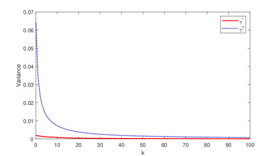
Figure 1: Variance comparison of stochastic gradient estimate: $g_{S_{l}}^{k}(\gamma=\gamma^{*})$ and $g_{S_{l}}^{k}(\gamma=1)$(x-axis is $k$, y-axis is variance of $g_{S_{l}}^{k}$)

As observed in Figure 1, the variances of $g_{S_{l}}^{k}(\gamma=\gamma^{*})$ and $g_{S_{l}}^{k}(\gamma=1)$ decrease as $k$ increases. In addition, the variance of $g_{S_{l}}^{k}(\gamma=\gamma^{*})$ is smaller than $g_{S_{l}}^{k}(\gamma=1)$. This result shows that the variance reduction effect of the new stochastic gradient estimate $(\gamma=\gamma^{*})$ is better than stochastic gradient estimate $(\gamma=1).$

$$g_{S_{l}}^{k}(\gamma) =\nabla f_{S_{l}}(w_{101})-\gamma(\nabla f_{S_{l}}(w_{k})-\frac{1}{n}\sum_{i=1}^{n}\nabla f_{i}(w_{k}))$$ (46)

$$k =0,1,2...100,l=1,2...100$$

$$Var(g_{S_{l}}^{k}(\gamma))=\frac{1}{100}\sum_{l=1}^{100}(g_{S_{l}}^{k}(\gamma)-\frac{1}{100}\sum_{l=1}^{100}g_{S_{l}}^{k}(\gamma))^{2},k=0,1,2...100$$ (47)

5.2 Experimental Result of Algorithm1 and Algorithm2

Figure 2 and Figure 3 plot the performance profile of SCGA, Algorithm1, CGVR and Algorithm2 on data sets of binary classification and regression. Two figures show that the Algorithm1 and Algorithm2 can converge faster than SCGA and CGVR.

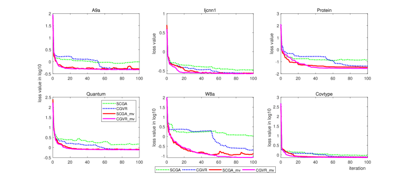
Figure 2: performance profiles of SCGA,CGVR,Algorithm1,Algorithm2 on the six data sets of binary classification (x-axis is times of iteration, y-axis is loss value in terms of log10)

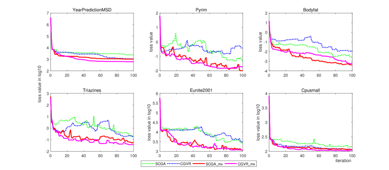
Figure 3: performance profiles of SCGA,CGVR,Algorithm1,Algorithm2 on the six data sets of regression (x-axis is times of iteration, y-axis is loss value in terms of log10)

Finally, Table 2 shows runtimes of the above experiments through 100 iterations. Note that runtime of Algorithm1 and Algorithm2 have no significant difference in runtime, compare to SCGA and CGVR.

Table 2: Runtime in 100 iterations

Dataset	SCGA	Algorithm1	CGVR	Algorithm2
A9a	4.53	4.60	3.92	4.26
Ijcnn1	5.86	5.75	5.13	5.09
Protein	16.12	15.89	14.54	14.59
Quantum	6.06	6.01	5.42	5.56
W8a	7.94	8.3	6.12	6.54 0
Covtype	61.53	62.47	54.48	55.50
YearPredictionMSD	49.85	50.71	44.90	46.34
Pyrim	0.10	0.14	0.12	0.14
Bodyfat	0.15	0.1	0.15	0.15 5
Triazines	0.14	0.21	0.15	0.23
Eunite2001	0.16	0.18	0.18	0.22
Cpusmall	1.20	1.19	1.02	1.05
Total	136.13	139.67	153.65	155.60

6 Conclusion

In this paper, we propose a new variance reduction stochastic gradient estimate. It is a more desirable estimate than estimate in SCGA and CGVR for its unbiasedness and minimal variance. Then we apply it to SCGA and CGVR, and propose two improved algorithms: Algorithm1 and Algorithm2. Next, the linear convergence rate of the new algorithms is proved under strong convexity and smoothness. Finally, we compare the convergence rate of the SCGA, Algorithm1, CGVR, Algorithm2 in numerical experiments. The results show that Algorithm1 and Algorithm2 have significant advantages in convergence rate than SCGA and CGVR. Besides, their runtime is not obvious difference.

References

- (1) L. Bottou, “Large-scale machine learning with stochastic gradient descent,” in Proceedings of COMPSTAT’2010. Springer, 2010, pp. 177–186.
- (2) T. Dozat, “Incorporating nesterov momentum into adam,” Proc. ICLR Workshop, pp. 1–4, 2016.
- (3) S. J. Reddi, S. Kale, and S. Kumar, “On the convergence of adam and beyond,” Proc. ICLR, pp. 1–23, 2018.
- (4) M. Schmidt, N. Le Roux, and F. Bach, “Minimizing finite sums with the stochastic average gradient,” Mathematical Programming, vol. 162, no. 1, pp. 83–112, 2017.
- (5) A. Defazio, F. Bach, and S. Lacoste-Julien, “Saga: A fast incremental gradient method with support for non-strongly convex composite objectives,” Advances in neural information processing systems, vol. 27, pp. 1646–1654, 2014.
- (6) R. Johnson and T. Zhang, “Accelerating stochastic gradient descent using predictive variance reduction,” Advances in neural information processing systems, vol. 26, 2013.
- (7) C. Kou and H. Yang, “A mini-batch stochastic conjugate gradient algorithm with variance reduction,” Journal of Global Optimization, pp. 1–17, 2022.
- (8) X.-B. Jin, X.-Y. Zhang, K. Huang, and G.-G. Geng, “Stochastic conjugate gradient algorithm with variance reduction,” IEEE Transactions on Neural Networks and Learning Systems, vol. 30, no. 5, pp. 1360–1369, 2018.
- (9) R. Fletcher and C. M. Reeves, “Function minimization by conjugate gradients,” The computer journal, vol. 7, no. 2, pp. 149–154, 1964.
- (10) E. Polak and G. Ribiere, “Note sur la convergence de méthodes de directions conjuguées,” Revue française d’informatique et de recherche opérationnelle. Série rouge, vol. 3, no. 16, pp. 35–43, 1969.
- (11) B. T. Polyak, “The conjugate gradient method in extremal problems,” USSR Computational Mathematics and Mathematical Physics, vol. 9, no. 4, pp. 94–112, 1969.
- (12) M. R. Hestenes and E. Stiefel, “Methods of conjugate gradients for solving,” Journal of research of the National Bureau of Standards, vol. 49, no. 6, p. 409, 1952.
- (13) Y. Liu and C. Storey, “Efficient generalized conjugate gradient algorithms, part 1: theory,” Journal of optimization theory and applications, vol. 69, no. 1, pp. 129–137, 1991.
- (14) Y.-H. Dai and Y. Yuan, “A nonlinear conjugate gradient method with a strong global convergence property,” SIAM Journal on optimization, vol. 10, no. 1, pp. 177–182, 1999.
- (15) D. Touati-Ahmed and C. Storey, “Efficient hybrid conjugate gradient techniques,” Journal of optimization theory and applications, vol. 64, no. 2, pp. 379–397, 1990.
- (16) Y. Hu and C. Storey, “Global convergence result for conjugate gradient methods,” Journal of Optimization Theory and Applications, vol. 71, no. 2, pp. 399–405, 1991.
- (17) J. C. Gilbert and J. Nocedal, “Global convergence properties of conjugate gradient methods for optimization,” SIAM Journal on optimization, vol. 2, no. 1, pp. 21–42, 1992.
- (18) Y.-H. Dai and C.-X. Kou, “A nonlinear conjugate gradient algorithm with an optimal property and an improved wolfe line search,” SIAM Journal on Optimization, vol. 23, no. 1, pp. 296–320, 2013.
- (19) W. W. Hager and H. Zhang, “A new conjugate gradient method with guaranteed descent and an efficient line search,” SIAM Journal on optimization, vol. 16, no. 1, pp. 170–192, 2005.
- (20) W. W. Hager and H. Zhang, “The limited memory conjugate gradient method,” SIAM Journal on Optimization, vol. 23, no. 4, pp. 2150–2168, 2013.
- (21) N. Andrei et al., Nonlinear conjugate gradient methods for unconstrained optimization. Springer, 2020.
- (22) Y. H. Dai, “Nonlinear conjugate gradient methods,” American Cancer Society.
- (23) T. Lidebrandt, Variance reduction three approaches to control variates. Matematisk statistik, Stockholms universitet, 2007.