A Gaussian Sliding Windows Regression Model for Hydrological Inference

Abstract

Statistical models are an essential tool to model, forecast and understand the hydrological processes in watersheds. In particular, the modeling of time lags associated with the time between rainfall occurrence and subsequent changes in streamflow, is of high practical importance. Since water can take a variety of flowpaths to generate streamflow, a series of distinct runoff pulses from different flowpath may combine to create the observed streamflow time series. Current state-of-the-art models are not able to sufficiently confront the problem complexity with interpretable parametrization, which would allow insights into the dynamics of the distinct flow paths for hydrological inference. The proposed Gaussian Sliding Windows Regression Model targets this problem by combining the concept of multiple windows sliding along the time axis with multiple linear regression. The window kernels, which indicate the weights applied to different time lags, are implemented via Gaussian-shaped kernels. As a result, each window can represent one flowpath and, thus, offers the potential for straightforward process inference. Experiments on simulated and real-world scenarios underline that the proposed model achieves accurate parameter estimates and competitive predictive performance, while fostering explainable and interpretable hydrological modeling.

1 Introduction

The hydrological processes that produce streamflow play key roles in determining the environmental effects of climate and land use changes. In particular, changes in climate or land use can trigger a complex series of nonlinear and interactive processes which can eventually impact the way in which watersheds partition, store, and release water, leading to potential changes in flood, landslide or drought risks (Dunn et al., 2010; Harman et al., 2011; Sawicz et al., 2014). Furthermore, water reservoirs and consistent streamflow are essential for the regulation of the water supply in both urban and rural areas (Janssen et al., 2021; Tang et al., 2009), as well as for sustainable energy production and continually healthy ecological habitats (Ahmad and Hossain, 2020; Zalewski et al., 2000). A deep understanding of how precipitated water becomes streamflow is of great importance and requires a sophisticated and interpretable statistical framework.

Hence we investigate the problem of inferring streamflow partitioning into different flowpaths such as overland flow, subsurface flow, and baseflow (Cornette et al., 2022; Kannan et al., 2007; McMillan, 2020; Nejadhashemi et al., 2009). While there exist many simple methods which can partition streamflow into fast surface flow versus slow baseflow (Nejadhashemi et al., 2009), the processes and reasoning behind this partitioning is usually lost. To prevent this, one could consider how input rainfall is partitioned into different flow paths. Hence, we consider a time series $\left(y_{t}\right)_{t\in T}$ of streamflow at a particular gauge and an input time series $\left(x_{t}\right)_{t\in T}$ of climate data on a common observational interval $T$. Given such data, a common approach is a lagged regression model following the concepts of auto-regressive moving-average with exogenous variables (ARIMAX, ARMAX) (Hyndman and Athanasopoulos, 2021). In contrast to these models, our problem does not involve lagged observations of the target $y_{t}$; instead, we seek to fully characterize the target time series via the lagged input time series. Further, we desire more interpretability and inferential power than is offered by ARIMAX models. For example, the maximum time interval for which the predictor has an impact on the response and the separation of flow pathways is of interest for watershed modeling.

A more closely related model in time series analysis is the finite distributed lag model (DLM) (Baltagi, 2022). Despite its roots in econometrics, the DLM has been extensively applied in environmental sciences (Chen et al., 2018; Peng et al., 2009; Rushworth et al., 2013; Warren et al., 2020). While ARIMAX mainly relies on the concept of ARIMA, i.e. it makes use of the lagged target variable $y_{t}$ as input, and only adds the present time point of the exogenous variable $x_{t}$, DLM predicts the target variable purely based on a distinct lagged input time series — the same setup that is pursued in this work. Basic DLM variants do not allow us to impose parametric assumptions on the shape of the regression parameter vector beyond simple singular shapes like geometrically decreasing patterns or polynomials (Almon, 1965; Eisner, 1960; Griliches, 1967), though recent work (Rushworth, 2018) extends the concept to B-splines in a Bayesian setting. Such DLM extensions permit a large variety of lag curve shapes, but do not make the separation between flow paths explicit. Crucially, then, they do not allow users to extract hydrologic inferences about distinct flow pulses.

Another economic model is adapted for hydrological inference by Giani et al. (2021), where the authors deploy the concept of cross-correlations in combination with a moving-average approach. Although their method has favorable properties to model the response time between rainfall events and flow pulses, it again does not allow a direct separation of the flow paths. Furthermore, correlation-based analyses do not allow straight-forward predictions on new test datasets.

An alternative to the approaches based on statistical time series models is to address the problem via systems of differential equations based on domain knowledge. In this category, Young (2006) describes transfer functions as a way to model dynamics in hydrological problems. A probabilistic model for travel time distributions of water under different soil conditions is proposed by Botter et al. (2010). Partial differential equation models, however, require an in-depth understanding of the application domain and potentially restrictive assumptions. Due to their complexity, interpretation is often not straight-forward. Finally, heavy numerical simulations are required, which may be resource and time prohibitive in large-scale experiments.

In contrast to further related works in the field of statistical modeling in hydrology, the methodology presented here focuses exclusively on the temporal relation between rainfall and streamflow in a given watershed. Spatial relationships between watersheds, as investigated by Roksvg et al. (2021), are beyond the scope of this article; nevertheless, the presented concept offers a foundation, which can be extended to include spatial information for gauged and ungauged catchments in future work and may complement existing large-scale analyses, such as that of Hare et al. (2021).

In this article, we present a parameterized, interpretable variant of lagged regression models for hydrological modelling: the Gaussian Sliding Window Regression model. It builds on the assumption that distinct flow paths (surface flow, sub-surface flow, etc.) provoke separable pulses of streamflow after rainfall events. These pulses are represented by multiple temporal windows, which weight the input $x_{t}$ at time points within the window via a Gaussian kernel. The output of each window is mapped to the target variable $y_{t}$ using a linear regression model. Compared to earlier Sliding Window Regression models (Davtyan et al., 2020; Khan et al., 2019; Janssen et al., 2021), the proposed method has major structural differences, which constitute the main novelties of our work:

1. We consider multiple, potentially overlapping windows representing distinct flow paths,

2. we use a parameterized kernel as model weights to allow straight-forward interpretations for hydrological inference, and

3. we allow windows not to cover the full interval between the maximum lag and the present time.

Our experimental evaluation involves both simulation and real-world experiments. The simulation study serves as a proof of concept for the model and validates the parameter estimation procedure. The application to two sets of real-world data demonstrates that the model achieves competitive predictive performance and has favorable properties for interpreting underlying hydrological processes.

2 Sliding Windows Regression Model

Our problem setup is based on a univariate input time series $x_{T}$ and a univariate target time series $y_{T}$ on a common, discrete time domain $T=[t_{\max}]$, where $[n]$ denotes the index set $\{0,\dots,n\}$. In the motivating application $x_{T}$ and $y_{T}$ represent rainfall and streamflow, respectively. The modeling goal is to represent the target value $y_{t}$ at time $t\in T$ based on time-lagged observations of $x_{[t]}$.

Our proposed model pursues the idea that the effect of precipitation on streamflow follows a mixture of $k$ kernels associated with temporal windows, each one characterizing a particular flow path (groundwater flow, sub-surface flow, or overland flow). Ultimately, we aim to represent the respective processes by weight vectors $\bm{w}^{(1)},\dots,\bm{w}^{(k)}\in\mathbb{R}^{t}$; each vector is over a range of lagged times and is associated with one flow path. Computing a weighted sum of the lagged time series $x_{[t]}$ with one such weight vector $\bm{w}^{(i)}$ delivers us an estimate for the amount of streamflow associated with the flow path $i\in\{1,\dots,k\}$ at time $t$. Summing the contributions gives the overall flow. To facilitate explanations, we present the model for the special case of only $k=1$ window first, and extend it to multi-window scenarios afterwards.

2.1 Single-window model

If only one flow path exists, we denote the associated weight vector by $\bm{w}\in\mathbb{R}^{t}$. By default, we require that all entries in $\bm{w}$ are non-negative, and that $\bm{w}$ is normalized, i.e. $\|\bm{w}\|_{1}=1$. Then, the gauged runoff $y_{t}$ is modeled by the weighted sum or the associated convolution

$$y_{t} =\beta\cdot\left(\sum\limits_{s=0}^{t}x_{t-s}w_{s}\right)+\varepsilon_{t}$$

$$=\beta\cdot\left(x_{[t]}\ast\bm{w}\right)+\varepsilon_{t},$$ (1)

with some multiplicative constant $\beta$ and an error term $\varepsilon_{t}$ assumed as Gaussian white noise. The symbol $\ast$ denotes the discrete convolution operator defined as

$$\bm{v}\ast\bm{z}=\sum\limits_{i=0}^{n}v_{n-i}z_{i}$$

for two vectors $\bm{v},\bm{z}\in\mathbb{R}^{n}$. Note that weight $w_{s}$ is applied to lag $s\in[t]$, i.e. $w_{s}$ denotes the weight applied to observation $x_{t-s}$ rather than $x_{s}$. The model parameter $\beta$ acts as a regression coefficient to adjust the scaling of the normalized weight vector $\bm{w}$. Since additional precipitation cannot lead to decreased streamflow, we additionally define $\beta$ to be positive, i.e. $\beta>0$. If applied in other domains, this restriction may be removed.

The assumption of independent errors $\varepsilon_{t}$ in model (1) (or its $k$-kernel generalization) is unrealistic for most real-world datasets where autocorrelated disturbances are common. Later, we describe a simple data transformation to address that complexity, however, and it is sufficient to proceed with the simpler model (1) for now.

2.1.1 Temporal windows

In practice, it is reasonable to assume that there exists a maximum time delay $s_{\max}$ between a water input pulse and the corresponding streamflow. Hence, the subset of lags with non-zero weights, $\{s:w_{s}>0\}$, is bounded above by $s_{\max}$, such that $w_{s}=0$ for all $s>s_{\max}$. On the other hand, water associated with slower flow paths may not reach the runoff gauge in less than a minimum time lag $s_{\min}\geq 0$, resulting in $w_{s}=0$ for $s<s_{\min}$. In essence, we define a temporal window as an interval of time lags, $W=[t-s_{\max},\dots,t-s_{\min}]\subseteq T$, and the corresponding window center lag (denoted as window location parameter) as

$$\delta=\frac{s_{\max}+s_{\min}}{2}>0.$$

The window size is by default assumed to be even-numbered and defined as $(s_{\max}-s_{\min})=2r$ for some window size parameter $r\in\mathbb{N}$, such that the number of time lags within the window, $\{s_{\min},s_{\min}+1,\dots,s_{\max}\}$, is $2r+1$.

Given such a window, the modeled response $y_{t}$ only depends on $x_{[t-s_{\max},t-s_{\min}]}$. We denote the subvector of a vector $\bm{v}\in\mathbb{R}^{n}$ with respect to the consecutive set of integer indices $\{i,i+1,\dots,j\}\subseteq[n]$ by $v_{[i,j]}=\left(v_{i},v_{i+1},\dots,v_{j}\right)$. For some index subset $S\subseteq\mathbb{N}$, time series segments are analogously abbreviated by $x_{S}=\left(x_{t}\right)_{t\in S}$ and treated as finite-dimensional vectors. Therefore, we can simplify the representation of the kernel weights to the subvector $\bm{\kappa}=w_{[s_{\min},\dots,s_{\max}]}\in\mathbb{R}^{2r+1}$. As a result, Eq. (1) results in the Sliding Window Regression (SWR) model with one window

$$y_{t}=\beta\cdot\left(x_{W}\ast\bm{\kappa}\right)+\varepsilon_{t}.$$ (2)

Note that the index of the kernel weights increase with the time lag, i.e., the first weight in $\bm{\kappa}$ corresponds to the most recent time point and the last weight corresponds to the most distant time point.

Graphically, the idea behind the SWR model for a univariate input $x_{[t]}$ can be visualized in Fig. 1: the target time series at time $t$, $y_{t}$, is predicted based on information from the input time series in window $W$, $x_{W}$.

Figure 1: Illustration of the Sliding Windows Regression model with $k=1$ window, which predicts $y_{t}=y_{70}$ based on $x_{W}$. On the time axis, the window $W=[40,60]$ is centered around $s=t-\delta=50$ and covers $2r+1=21$ time points. The window location parameter $\delta$ and the window size parameter $l$ are given by $\delta=20$ and $r=10$, respectively.

2.1.2 Gaussian Sliding Windows Regression Model

In the Gaussian SWR model, we introduce a parametrization to the window kernel: under the assumption that the time delay between the rainfall event and the resulting change in the streamflow is approximately Gaussian distributed, the weights $\bm{w}$ take the shape of a Gaussian probability density function centered around $s=t-\delta$ on the time axis. Since the time series is only measured at discrete time points, the Gaussian kernel is discretized by applying a step function, such that

$$\kappa_{i}=\frac{1}{C}\int\limits_{i-\frac{1}{2}}^{i+\frac{1}{2}}\phi(t;0,\sigma^{2})\ dt,$$

where $\phi(.,\mu,\sigma^{2})$ denotes the probability density function of a Gaussian distribution with mean $\mu$ and variance $\sigma^{2}>0$, the kernel indices $i\in\{-r,\dots,r\}\subset\mathbb{Z}$ are relative to the position of the window center $\delta$ so that the distribution has mean $\mu=0$, and $C$ denotes the normalization constant

$$C=\sum\limits_{i=-r}^{r}\int\limits_{i-\frac{1}{2}}^{i+\frac{1}{2}}\phi(t;0,\sigma^{2})\,dt\\ =\int\limits_{i-r-\frac{1}{2}}^{i+r+\frac{1}{2}}\phi(t;0,\sigma^{2})\,dt.$$

Examples for $r\in\{1,3,6\}$ and $\sigma=\frac{r}{3}$ are depicted in Fig. 2.

Figure 2: Examples for Gaussian shaped window kernels (weights). $r$ denotes the window size, centered around $s$.

Obviously, there exists a strong relation between the variance $\sigma^{2}$ and the window size $r$: even though the definition of kernel weights implies that non-zero weights occur for arbitrary size $r$, weights decay exponentially with their distance from the kernel center $s$. The number of model parameters characterizing the window kernel, hence, reduces to $\delta$ and $\sigma$. By default, the window is set to range from $s_{\min}=\lfloor s-3\sigma\rfloor$ to $s_{\max}=\lceil s+3\sigma\rceil$, which is guaranteed to cover more than $99\%$ of the probability mass. Note that, while $s$ does not always match with a time point measured in the time series, $s_{\min}$ and $s_{\max}$ are rounded to the previous and next measured time point, respectively. As a consequence, estimation of the window width is done via the continuous parameter $\sigma$, from which $r\approx 3\sigma$ follows. Based on this relation, we will use the parameter $\sigma$ instead of $r$ in the remainder of this article.

In the special case that $\sigma$ is very small and $r$ becomes $0$, the window length is $1$ and the full probability mass of the kernel accumulates in the window center $\delta$. However, since $\delta$ may be located between two observations of the input time series, the full probability mass is assigned to the closest measured time point in such cases, by definition.

2.1.3 Truncation and boundary conditions

Due to the fundamental condition that $s_{\min}\geq 0$ and $s_{\max}\leq t$, it follows that the Gaussian SWR model cannot be evaluated for arbitrary parameter combinations of $\delta$ and $\sigma$. The restriction $s_{\max}\leq t$ is less prohibitive in practice for longer time series and merely leads to $y_{t}$ not being predictable for $t<s_{\max}$. Hydrological application typically have time lags $\delta$ in the range of a few days, weeks or months, hence the impact of this restriction is negligible for a sufficiently long time series spanning over multiple years.

On the other hand, short time lags $\delta$ are highly relevant in practice. Under extremely wet conditions in low permeability catchments, it can be assumed that water from rainfall will almost immediately lead to changes in streamflow. Since $s_{\min}=\delta-r\geq 0$ implies that $\delta\geq r$, the lag of the time point with the maximum weight $w_{\delta}$ must not exceed the window size parameter $r$. Hence, the kernel requires modification to handle situations with fast-flowing water reaching its peak at a small time lag, i.e. $\delta<r$.

For this purpose, we truncate the kernel $\bm{\kappa}$ by $\tau=\max\{0,r-\delta\}$ time steps exceeding the upper limit $t$ on the time axis: the truncated kernel $\bm{\kappa}^{\tau}$ is given by

$$\bm{\kappa}^{\tau}\propto\kappa_{[1,(2r+1-\tau)]}.$$

The truncation results from ablating $\tau$ vector entries on the right side of $\bm{\kappa}$. As illustrated in Fig. 3, the truncated kernel represents a discretization of a truncated Gaussian density function.

Figure 3: Example for a truncated Gaussian shaped window kernel. In this example, window parameters $\delta=3$ and $r=6$ require a truncation by $\tau=3$ time points.

Note, however, that truncation has effects on the interpretation of the model parameters: while $\delta$ still indicates the time lag with the highest peak in model weights, it does not indicate the central lag of the window on the time axis anymore. Further, the right-truncated Gaussian distribution is no longer symmetric with respect to the temporal window, and hence, the distribution mean shifts to the left.

2.2 Multi-window model

Assuming multiple different (potentially overlapping) windows allows the model to account for distinct effects on the current target $y_{t}$. For this purpose, we extend our method from a single-window model to a mixture of $k$ kernels, which is related to the density resulting from a mixture of probability distributions (Everitt et al., 1981). For a given window $i\in\{1,\dots,k\}$, we use the same notation as in the single-window case for the window and kernel parameters with an added index $i$ denoting the window number: $\delta_{i}$, $r_{i}$, $s_{\min}^{(i)}$, $s_{\max}^{(i)}$ and $\sigma_{i}$. The Gaussian SWR model with multiple windows $W_{1},\dots,W_{k}$ is given as a direct generalization of Eq. 2 by

$$y_{t}=\sum_{i=1}^{k}\beta_{i}\cdot\left(x_{W_{i}}\ast\bm{\kappa}^{(i)}\right)+\varepsilon_{t},$$ (3)

where the regression parameters $\beta_{1},\dots,\beta_{k}\geq 0$ act as window weights. In summary, the Gaussian SWR model with $k$ windows contains the following parameters

• $k$ regression parameters ($\beta_{1},\dots,\beta_{k}$), $\beta_{i}\in\mathbb{R}^{+}$,

• $k$ lag parameters ($\delta_{1},\dots,\delta_{k}$), $\delta_{i}\in\mathbb{R}^{+}$, and

• $k$ kernel variance (size) parameters ($\sigma_{1}^{2},\dots,\sigma_{k}^{2}$), $\sigma_{i}\in\mathbb{R}^{+}$.

The concept of a Gaussian SWR model with multiple windows is illustrated in Fig. 4: a target value $y_{t}$ is predicted by multiple windows accumulating information in $x_{[t]}$ over different time intervals. Hence, the joint kernel forms a multi-modal distribution and can be interpreted as a kernel density estimator describing a more general mixture distribution of Gaussian and truncated Gaussian kernels. As depicted in Fig. 5, the combined kernel represents a linear combination of the single window kernels $\bm{\kappa}^{(i)}$, $i=1,\dots,k$. Under the assumption that each window has a distinct center point $\delta_{i}$ (otherwise, identifiability of the parameters might not be given), without loss of generality we can order the location parameters such that $\delta_{1}<\delta_{2}<\dots<\delta_{k}$.

Figure 4: Illustration of the Sliding Windows Regression model with $k=2$ windows, which predicts $y_{t}=y_{70}$ based on $x_{W_{1}}$ and $x_{W_{2}}$. On the time axis, the window $W_{1}=[40,60]$ is centered around $s_{1}=50$ and covers $2r_{1}+1=21$ time points, while window $W_{2}=[10,50]$ is centered around $s_{2}=30$ and covers $2r_{2}+1=41$ time points. The window location parameters and the window size parameters are given by $\delta_{1}=20$, $\delta_{2}=40$ and $\sigma_{1}=3.25$, $\sigma_{2}=6.5$, leading to $r_{1}=10$, $r_{2}=20$, respectively.

2.2.1 Parameter interpretation

By definition, the number of windows $k$ models the number of underlying, separable flow paths.

Since single-window kernels $\bm{\kappa}$ are normalized, regression parameters (window coefficients) $\beta_{1},\dots,\beta_{k}$ act as weights among the kernels. For practical evaluations, they may be converted into proportions representing the relative impacts of the underlying flow paths.

For symmetric windows, the location parameter $\delta_{i}$ and the width $\sigma_{i}$ of kernel $i$ indicate the mean and the standard deviation, respectively, of the time lag between precipitation and a change in streamflow. Thus, a direct estimate of the expected time delay between rainfall events and the resulting impact on the gauged runoff is possible for each flow path.

Figure 5: Examples for a mixture of window kernels (weights): kernel $\bm{\kappa}_{1}$ represents a truncated Gaussian, while kernel $\bm{\kappa}_{2}$ has a Gaussian shape. The combined window $\beta_{1}\bm{\kappa}_{1}+\beta_{2}\bm{\kappa}_{2}$ show a representation of the mixture model induced by the Gaussian SWR model.

2.3 Information criteria

Based on the definition and the model assumptions of the proposed Gaussian SWR model, the model errors are given by

$$\varepsilon_{t}=y_{t}-\beta_{1}\cdot\left(x_{W_{1}}\ast\bm{\kappa}^{(1)}\right)-\dots-\beta_{k}\cdot\left(x_{W_{k}}\ast\bm{\kappa}^{(k)}\right),$$

and follow a Gaussian white noise process. Hence, the log-likelihood $\log L(\bm{\beta},\bm{\delta},\bm{\sigma};x_{T},y_{T})$ is tractable and matches the log-likelihood of ordinary multiple linear regression models.

Using the log-likelihood and the number of parameters, Akaike’s Information Criterion (AIC) (Akaike, 1974) can be computed by

$$\text{AIC}=-2\log L(\bm{\beta},\bm{\delta},\bm{\sigma};x_{T},y_{T})+6k,$$

since the number of model parameters in a $k$-window model aggregates one regression parameter, one window location parameter, and one window width parameter for each of the $k$ windows. Analogously, the Bayesian Information Criterion (BIC) (Schwarz, 1978) is given as

$$\text{BIC}= -2\log L(\bm{\beta},\bm{\delta},\bm{\sigma};x_{T},y_{T})+\log(|T|)\cdot 3k,$$

where $|T|$ is the number of observed time points (number of samples).

2.4 Model training & implementation

In a training dataset, let $y_{T}$ denote the observed values of the target time series, and let $\hat{y}_{T}$ denote the predictions. Given a loss function $\ell(y_{T},\hat{y}_{T}(x_{T};\bm{\beta},\bm{\delta},\bm{\sigma}))$, model training involves an iterative optimization procedure outlined in Alg. 1. In each iteration $i=1,\dots,k_{\max}$, one new window is added to the model and its parameters are optimized using the gradient-free BOBYQA algorithm (Powell, 2009). To optimally exploit information from window positions detected in previous iterations, the initialization for the new window location parameter $\delta$ explores multiple options collected in a set $\bm{\Theta}^{(i)}$. For instance, center points between previous windows, $\frac{\delta_{j-1}^{(i-1)}+\delta_{j}^{(i-1)}}{2}$ for $j\in\{2,\dots,i-1\}$, may be part of $\bm{\Theta}^{(i)}$, along with new points outside the range of previous windows, $0$ and $\delta_{i-1}^{(i-1)}+\zeta$, where $\zeta\in\{1,5,10\}$. The regression parameters $\bm{\beta}$ and variance parameters $\bm{\sigma}$ are initialized by distributing the previous cumulative weights and variances equally across all new windows. The training procedure continues until the defined number of iterations $k_{\max}$ (which equals the maximum number of windows) is reached.

In the target function for the BOBYQA algorithm, parameters are optimized over the full range of real numbers ($\beta$) or positive real numbers ($\delta$,$\sigma$), respectively. Since no additional constraints are introduced, truncated as well as non-truncated kernels may be obtained. In the boundary case of $\delta=0$, a maximum level of truncation is reached, which reduces the kernel to the lower half of a Gaussian distribution density. If $\sigma=0$, the full probability mass of the kernel is reduced to the closest time lag.

If the number of windows is not known a-priori, an upper bound $k_{\max}$ must be defined, and the hyperparameter $k$ will be selected by choosing the best among all $k_{\max}$ iterations based on an information criterion $IC$ representing either AIC or BIC.

set window counter $i\leftarrow 0$

do

     set $i\leftarrow i+1$

     if i = 1 then

         $\bm{\beta}^{(1)}\leftarrow\bm{\delta}^{(1)}\leftarrow\bm{\sigma}^{(1)}\leftarrow 1$

         run BOBYQA algorithm initialized with $\bm{\beta}^{(1)}$, $\bm{\delta}^{(1)}$, $\bm{\sigma}^{(1)}$:

$$(\bm{\beta}^{(1)},\bm{\delta}^{(1)},\bm{\sigma}^{(1)})\leftarrow\underset{(\bm{\beta},\bm{\delta},\bm{\sigma})}{\arg\min}~{}\ell\left(y_{t},\hat{y}_{T}(x_{T};\bm{\beta},\bm{\delta},\bm{\sigma})\right)$$

     else

         initialize new regression and window size parameter:

         $\bm{\beta}^{(i)}\leftarrow\frac{\|\bm{\beta}^{(i-1)}\|_{1}}{i},$

         $\bm{\sigma}^{(i)}\leftarrow\frac{\|\bm{\sigma}^{(i-1)}\|_{1}}{i}.$

         for $d_{j}^{(i)}$ in a set of initialization points $\bm{\Theta}^{(i)}$ do

              try initialization of $\bm{\delta}^{(i)}$:

$$\bm{\delta}^{(i,j)}\leftarrow\left(\bm{\delta}^{(i-1)},d^{(i)}_{j}\right)$$

              run BOBYQA algorithm initialized with $\bm{\beta}^{(i)}$, $\bm{\delta}^{(i,j)}$, $\bm{\sigma}^{(i)}$:

$$(\bm{\beta}^{(i,j)},\bm{\delta}^{(i,j)},\bm{\sigma}^{(i,j)})\leftarrow\underset{(\bm{\beta},\bm{\delta},\bm{\sigma})}{\arg\min}~{}\ell\left(y_{t},\hat{y}_{T}(x_{T};\bm{\beta},\bm{\delta},\bm{\sigma})\right)$$

         end for

         set $\left(\bm{\beta}^{(i)},\bm{\delta}^{(i)},\bm{\sigma}^{(i)}\right)\leftarrow\left(\bm{\beta}^{(i,J)},\bm{\delta}^{(i,J)},\bm{\sigma}^{(i,J)}\right)$, where $J$ optimizes the information criterion $IC$:

$$J=\underset{j}{\arg\min}~{}IC\left(y_{T},\hat{y}_{T}(x_{T};\bm{\beta}^{(i,j)},\bm{\delta}^{(i,j)},\bm{\sigma}^{(i,j)}),i\right).$$

     end if

while $i<k_{\max}$

return $\bm{\beta}^{(I)},\bm{\delta}^{(I)},\bm{\sigma}^{(I)}$, such that information criterion $IC$ is optimized:

$$I=\underset{i}{\arg\min}~{}IC\left(y_{T},\hat{y}_{T}(x_{T};\bm{\beta}^{(i)},\bm{\delta}^{(i)},\bm{\sigma}^{(i)}),k\right).$$

Algorithm 1 Train a Gaussian Sliding Windows Regression model

The Gaussian SWR model is implemented in R version 4.3.0 (R Core Team, 2022). The implementation is publicly available on GitHub. The BOBYQA algorithm from the package nloptr (Johnson, 2021) is used to optimize the model parameters of the Gaussian SWR by derivative-free quadratic approximations. By default, the loss function $\ell(.,.)$ refers to the negative log-likelihood, $-\log L(.,x_{T},y_{T})$. As stopping criterion, the absolute tolerance of the function values (ftol_abs) is set to $10^{-8}$. During optimization, all parameters are bounded below by $0$, while no upper bound is provided.

2.5 Autocorrelated residuals

Due to the time series aspect of precipitation and runoff data, we expect that model input and model output are both individually affected by autocorrelation. Even under a perfect selection of model parameters and no model misspecification, we expect that autocorrelation should be present in the residuals of the Gaussian SWR model, since both input and output time series may have measurement errors correlated with time. This aspect violates the requirements of ordinary least squares regression and may distract evaluation metrics such as root mean squared error. Thus, we aim to resolve such issues by adapting the estimation procedure proposed by Cochrane and Orcutt (1949) in the context of ordinary least squares models.

Suppose the errors $\varepsilon_{t}$ in the model (3) follow an autoregressive process of lag 1, i.e., AR(1), so that

$$\varepsilon_{t}=\varphi\varepsilon_{t-1}+\eta_{t},$$ (4)

where $\eta_{t}$ is Gaussian white noise (instead of $\varepsilon_{t}$ in Eq. (3)), and $\varphi\in(-1,1)$. From Eq. (3) and (4), it follows that

$$y_{t}=\sum_{i=1}^{k}\beta_{i}\cdot\left(x_{W_{i}}\ast\bm{\kappa}^{(i)}\right)+\varphi\varepsilon_{t-1}+\eta_{t},$$

leading to

$$y_{t}-\varphi y_{t-1}=\sum_{i=1}^{k}\beta_{i}\cdot\left(\left(x_{W_{i}}-\varphi x_{W_{i}-1}\right)\ast\bm{\kappa}^{(i)}\right)+\eta_{t},$$ (5)

where $W_{i}-1=[t-s_{\max}^{(i)}-1,\dots,t-s_{\min}^{(i)}-1]$ denotes the element-wise time shift of the interval $W_{i}$. Here, we are exploiting the linearity of the convolution operator. Hence, given $\varphi$, the model can be written as an ordinary least squares model with uncorrelated errors $\eta_{t}$:

$$\tilde{y}_{t}=\sum_{i=1}^{k}\beta_{i}\cdot\left(\tilde{x}_{W_{i}}\ast\bm{\kappa}^{(i)}\right)+\eta_{t},$$

where the transformation $\tilde{z}_{t}=z_{t}-\varphi z_{t-1}$ can be applied a-priori as part of the preprocessing procedure on both variables $x_{t}$ and $y_{t}$.

For the Gaussian SWR model, we adapt the Cochrane-Orcutt procedure to estimate $\varphi$ and the optimal model parameters:

• estimate model parameters $\bm{\beta},\bm{\delta},\bm{\sigma}$ from the original model using $x_{t}$ and $y_{t}$ (i.e., set $\varphi=0$),

• estimate $\varphi$ from the model residuals,

• apply transformation $\tilde{z}_{t}=z_{t}-\varphi z_{t-1}$ and re-estimate model parameters $\bm{\beta},\bm{\delta},\bm{\sigma}$ from the transformed variables $\tilde{x}_{t}$, $\tilde{y}_{t}$.

Finally, the same concept also holds for more general AR($m$)-processes with $m>1$. However, the transformation leads to a loss of $m$ time points (samples) in the training dataset.

2.6 Uncertainty quantification

Minimizing the negative log-likelihood with respect to $(\bm{\beta},\bm{\delta},\bm{\sigma})$ gives maximum-likelihood estimates of the model parameters. Large-sample theory implies the errors in the estimators have an approximate multivariate Gaussian distribution with mean $\bm{0}$ (asymptotically unbiased) and an approximate covariance matrix $\mathcal{I}^{-1}$, where

$$\mathcal{I}(\bm{\beta},\bm{\delta},\bm{\sigma})=\frac{\partial^{2}}{\partial(\bm{\beta},\bm{\delta},\bm{\sigma})^{2}}\left(-\log L(\bm{\beta},\bm{\delta},\bm{\sigma};\bm{x},\bm{y})\right)$$

denotes the observed information. The Hessian can be obtained numerically via the R package numDeriv (Gilbert and Varadhan, 2019). The diagonal elements of $\mathcal{I}^{-1}$ lead to standard errors, which provide the uncertainty quantification reported below for the two watersheds studied. These watersheds have very long time series to support the asymptotic argument.

3 Simulation Study

In a simulation study, the proposed Gaussian SWR model will be validated in controlled scenarios based on real-world input data and simulated targets.

3.1 Experimental Setup

Precipitation data $x_{T}$ is used from the Koksilah River watershed which is located in Cowichan, British Columbia, Canada, while an artificial target variable $y_{T}$ is sampled based on Eq. (3). The model parameters $\bm{\beta}$, $\bm{\delta}$ and $\bm{\sigma}$ are randomly generated for this purpose, along with Gaussian white noise errors $\varepsilon_{t}\sim N(0,\rho^{2})$. The error variance $\rho^{2}$ is scaled with respect to the explained variance of the model in order to steer the complexity of the particular setups. The distributions of the model parameters are described further below.

In all of the following setups, the model parameters of the Gaussian SWR model were estimated on a training set comprising a time series of the first 29 hydrological years. The test set consisted of the remaining 10 time series of hydrological years, which corresponds to an approximate 75%/25% split of the dataset.

The primary factors steering the difficulty associated with a setup in the simulation study are:

1. the (ground truth) number of windows $k^{\text{gt}}$ — the dimensionality and complexity of parameter estimation increases with the number of windows,

2. the pairwise overlap between (ground truth) windows on the time axis — a higher overlap leads to a decrease in the separability of windows, and

3. the level of measurement noise $\rho^{2}$ applied, given by the noise rate (relative to the explained variance of the model).

While $k^{\text{gt}}$ and $\rho$ are systematically varied, the overlap of windows is a result from the random sampling of ground truth model parameters.

We employ 15 distinct setups (five 1-, 2-, and 3-window setups, respectively). Each setup uses a set of parameters independently sampled from $\delta_{i}\sim U(0,20)$, and $\sigma_{i},\beta_{i}\sim U(0,5)$ for any $i\in\{1,\dots,k\}$, where $U(a,b)$ denotes a uniform distribution on the interval $[a,b]$. Each 1-, 2- and 3-window setup is repeated at 5 distinct levels of measurement noise $\alpha\in\{0.05,0.25,0.5,0.75,0.95\}$ to control the error relative to the signal, for a total of 75 simulation experiments.

Given a noise level $\alpha$, the measurement noise is added as follows: After evaluating the deterministic terms in Eq. (3) with the given model parameters, denoted as $\hat{y}_{T}$, we compute the associated sample variance $\text{Var}(\hat{y}_{T})$. Gaussian white noise with standard deviation $\rho=\alpha\cdot\sqrt{\text{Var}(\hat{y}_{T})}$ is simulated and added to construct $y_{T}=\hat{y}_{T}+\varepsilon_{T}$.

The resulting variance of $y_{T}$ can be expressed as $\text{Var}(y_{T})=(1+\alpha^{2})\text{Var}(\hat{y}_{T})$. Thus, $\alpha$ represents the relative noise level with respect to the explained standard deviation. This induces an upper bound on the $R^{2}$ score (Kuhn and Johnson, 2019) achievable by any predictor given $x_{T}$ and $y_{T}$: a perfect model $\hat{y}_{t}$ would achieve an $R^{2}$ score of

$$R^{2}\left(y_{T},\hat{y}_{T}\right) =1-\frac{\|y_{T}-\hat{y}_{T}\|_{2}^{2}}{\|y_{T}-\bar{y}\bm{1}\|_{2}^{2}}$$

$$=1-\frac{\text{Var}(\varepsilon_{T})}{\text{Var}(y_{T})}$$

$$=1-\frac{\alpha^{2}\text{Var}(\hat{y}_{T})}{(1+\alpha^{2})\text{Var}(\hat{y}_{T})}$$

$$=1-\frac{\alpha^{2}}{1+\alpha^{2}},$$ (6)

where $\bar{y}$ denotes the mean of $y_{T}$ across $T$, and $\bm{1}$ denotes a vector of ones. All noise levels $\alpha$ and associated $R^{2}$ scores are shown in Table 1.

Table 1: Noise levels and associated maximum $R^{2}$ scores (upper bound for predictive model performance).

	noise level $\alpha$	maximum $R^{2}$
1	0.05	0.998
2	0.25	0.941
3	0.5	0.8
4	0.75	0.64
5	0.95	0.526

3.2 Evaluation Metrics

In order to evaluate the Gaussian SWR model, we deploy evaluation metrics to assess both the accuracy of parameter estimation and the predictive performance. To facilitate the assessment of the estimated parameters, we introduce the notion of overlap between two weight vectors with equal dimensions, $\bm{w}^{(1)},\bm{w}^{(2)}\in\mathbb{R}^{t}$ as follows:

$$O(\bm{w}^{(1)},\bm{w}^{(2)})=\sum\limits_{s=1}^{t}\min\{w_{s}^{(1)},w_{s}^{(2)}\}.$$

Hence, in a functional setting, the overlap would describe the area covered by the minimum of both kernel functions; in our discretized scenario, the integral is replaced by a sum. Since both weight vectors are positive and sum to 1 due to the normalization condition, the overlap will be in $[0,1]$ and reaches $1$ only if both weight vectors are exactly equal.

We group the evaluation criteria applied to our model results into two categories:

• Kernel overlap: When combining all estimated windows to a joint weight vector, the overlap between the full predicted and the ground truth kernels is assessed (including the weighting of windows by regression parameters $\bm{\beta}$). In particular, we compute the overlap $O(\hat{\bm{\theta}},\bm{\theta})$, where $\hat{\bm{\theta}}=(\hat{\bm{\beta}},\hat{\bm{\delta}},\hat{\bm{\sigma}})$, and $\bm{\theta}=(\bm{\beta},\bm{\delta},\bm{\sigma})$, respectively. Thus, the combined kernel overlap evaluates the quality of overall parameter estimation, including the regression parameters $\bm{\beta}$.

• Predictive performance: Conventional regression metrics are used to evaluate the predictive performance of the model on the test set (Kuhn and Johnson, 2019). These include the root mean squared error (RMSE), as well as the coefficient of determination ($R^{2}$) on the test set. The latter is also known as Nash-Sutcliffe Efficiency (NSE) in hydrology (Nash and Sutcliffe, 1970) and is introduced in Eq. (6). In addition, the Kling-Gupta efficiency (KGE) is a performance metric used in hydrology which, unlike the NSE, independently encourages predictions to match the variability of observations, thereby removing the tendency of NSE to underestimate high flows and overestimate low flows (Gupta et al., 2009). It uses the following formulation:

  $$1-\sqrt{(r-1)^{2}+\left(\frac{\sigma_{\hat{y}_{T}}}{\sigma_{y_{T}}}-1\right)^{2}+\left(\frac{\mu_{\hat{y}_{T}}}{\mu_{y_{T}}}-1\right)^{2}},$$

  where $r$ denotes the Pearson correlation coefficient between $y_{T}$ and $\hat{y}_{T}$, $\mu$ represents the respective means, and $\sigma$ represents the respective standard deviations. All performance metrics are implemented using the R package hydroGOF (Mauricio Zambrano-Bigiarini, 2020).

3.3 Results for uncorrelated errors

In the first step, we evaluate the predicted kernels obtained from training the Gaussian SWR model in each setup specified above. We distinguish two scenarios: fixed $k$ indicates that the number of windows $k$ is fixed to the ground truth number of windows $k^{\text{gt}}$, i.e. no hyperparameter selection is performed. On the contrary, variable $k$ indicates that no information about $k$ is provided a priori, i.e. the model applies a maximum of $k_{\max}=3$ windows and selects $k$ based on the best BIC.

Fig. 6 compares the ground truth and estimated kernels for the middle noise level $\alpha=0.5$ in each setup. Dotted vertical lines indicate the true or estimated window centers $\delta_{i}$ along the time axis. In all 1-window and 2-window setups, window positions and sizes were accurately predicted. In the 3-window setups, dominant peaks and general shapes are reconstructed in all scenarios. Among the less dominant kernels, minor deviations in position of the window center and the regression parameters are visible. The worst fit is observed in setup no. 13, where the weight of the second window is over-estimated, while the weight of the first window is under-estimated in magnitude. Nevertheless, the combined kernel matches with the ground truth very accurately, and the general separation of the windows is acceptable.

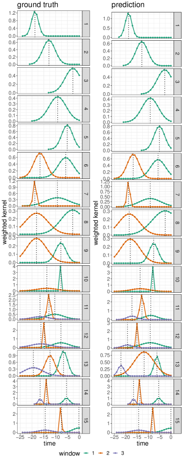
Figure 6: Ground truth versus predicted kernels (noise level $\alpha=0.5$). The number of windows was selected as a model hyperparameter.

Beyond visual comparison, Table 2 provides an overview of computed metrics based on predicted and true parameters. Overall, all setups achieve excellent overlaps with the ground truth kernels (almost 1.0, around 0.99 and approximately 0.97 for 1-window, 2-window, and 3-window models, respectively). Thus, the reconstruction of the overall weighted kernel is at a high level across all simulated setups.

Table 2: Parameter estimation errors for 1-, 2- and 3-window setups. All results are averaged over all noise levels.

setup no.	overlap
1-window setups
1	1.00
2	1.00
3	1.00
4	1.00
5	1.00
mean	1.00
2-window setups
6	0.99
7	0.99
8	0.99
9	0.99
10	0.99
mean	0.99
3-window setups
11	0.97
12	0.96
13	0.96
14	0.98
15	0.97
mean	0.97

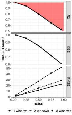
Figure 7: Predictive performance summaries for 1-, 2- and 3-window setups by noise level. All results are averaged over the 5 distinct simulated parameter setups.

Having observed the high accuracy of parameter identification in the well-separated scenarios of the simulation experiment, we further investigate the predictive performance of the models with respect to the target variable on the test set. Figure 7 illustrates the corresponding $R^{2}$, KGE, and RMSE scores obtained by the estimated Gaussian SWR models. In agreement with the observations made on the quality of parameter estimation, the predictive performance remains at a high level and is mainly affected by the noise levels. For the $R^{2}$ score, the upper bounds in Table 1 are indicated by a red region, which cannot be reached at the given noise level. The achieved $R^{2}$ values are close to the upper bounds across all model setups, and hence the estimated models obtain almost optimal prediction accuracy on the test set.

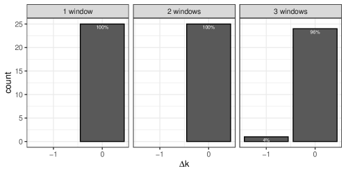
Figure 8: Histogram of hyperparameter estimation error $\Delta k$ across all setups.

To guarantee interpretability of the model parameters, an accurate estimation of the number of windows $k$ is crucial. To investigate the accuracy of the hyperparameter selection procedure, Fig. 8 shows a histogram of errors $\Delta k=k-k^{\text{gt}}$, where $k$ is the predicted number of windows according to BIC values. For $k^{\text{gt}}=1$ and $k^{\text{gt}}=2$, all predicted models select $k=1$ and $k=2$ windows, respectively. Thus, correct hyperparameters are selected in these setups. For $k^{\text{gt}}=3$, an error of $-1$ (under-estimation by one window) occurs in $1$ out of the $25$ setups ($4\%$). The affected setup is 11 at a high noise level of $\alpha=0.75$, where for one repeat experiment only two non-dominant windows are erroneously combined into one.

3.4 Results for autocorrelated errors

To account for more general error structures, we repeat the above experiment but with response data simulated according to autocorrelated AR(1) errors $\varepsilon_{t}$. We make use of the R function arima.sim from package forecast (Hyndman and Athanasopoulos, 2021) to simulate AR(1) noise with a given standard deviation $\rho$, which represents the sample variance $\text{Var}(\hat{y}_{T})$ and the noise levels $\alpha$ from Table 1 analogous to the case of uncorrelated errors. Internally, the function constructs i.i.d. errors $\eta_{t}$ with the given standard deviation $\rho$, which are then transformed to form an AR(1) process. The true autoregressive parameter $\varphi$ is set to 0.5 throughout.

In practice, autocorrelation has to be assessed and the autoregressive parameter $\varphi$ estimated when we extend the Gaussian SWR model using the Cochrane-Orcutt procedure. As a proof-of-concept, the Durbin-Watson test for autocorrelated model errors is performed to assess the residuals before and after the Cochrane-Orcutt data transformation. As expected, model fits with no Cochrane-Orcutt transformation deliver p-values below $0.01$ (rejecting the null hypothesis of no autocorrelation) for all 75 setups. The average absolute estimation error of the parameter $\varphi$ is $0.007$ across all setups, suggesting highly accurate estimation. After applying the Cochrane-Orcutt procedure, however, 73 out of the 75 setups lead to residuals with with p-values above $0.1$, which provides no evidence for violation of the assumption of uncorrelated residuals. The two remaining setups have only small residual correlation, $0.04$ and $0.02$, respectively.

Under the autocorrelated error model, the upper bounds for the $R^{2}$ scores achievable by the model must be modified: Since $\text{Var}(\varepsilon_{1})=\text{Var}(\eta_{1})$ and $\text{Var}(\eta_{t})=\alpha^{2}\text{Var}(\hat{y}_{T})$, it holds that

$$\text{Var}(\varepsilon_{t}) =\varphi^{2}\text{Var}(\varepsilon_{t-1})+\text{Var}(\eta_{t})$$

$$=\varphi^{4}\text{Var}(\varepsilon_{t-2})+\varphi^{2}\text{Var}(\eta_{t-1})+\text{Var}(\eta_{t})$$

$$=\dots=\sum\limits_{i=0}^{t-1}\varphi^{2i}\text{Var}(\eta_{t-i})$$

$$=\underbrace{\frac{1-\varphi^{2(t-1)}}{1-\varphi^{2}}}_{\xi}\alpha^{2}\text{Var}(\hat{y}_{T}).$$

It holds that $\xi\approx\frac{1}{1-\varphi^{2}}$ for longer time series. As a result, the maximum achievable $R^{2}$ score under the AR(1) model errors is given by

$$R^{2}(y_{T},\hat{y}_{T}) =1-\frac{\xi\alpha^{2}\text{Var}(\hat{y}_{T})}{(1+\xi\alpha^{2})\text{Var}(\hat{y}_{T})}$$

$$=\frac{1}{1+\xi\alpha^{2}}.$$

For the given noise levels $\alpha$, the maximum $R^{2}$ scores for the autocorrelated simulations are presented in Table 3. Results obtained for the experimental setups are shown in Fig. 9. As with the uncorrelated model setups, the $R^{2}$ scores almost reach the theoretical upper bound.

Table 3: Noise levels and associated maximum $R^{2}$ scores (upper bound for predictive model performance) in the autocorrelated setups.

	noise level $\alpha$	maximum $R^{2}$
1	0.05	0.997
2	0.25	0.923
3	0.5	0.75
4	0.75	0.571
5	0.95	0.454

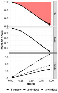
Figure 9: Predictive performance summaries for 1-, 2- and 3-window setups by noise level in the autocorrelated setup

Finally, the hyperparameter selection under the autocorrelated model setup is demonstrated in Fig. 10. Overall, the number of windows $k$ selected via BIC matches the ground truth in all 1-window setups, overestimates by 1 for 4 out of 25 of the 2-window setups, and underestimates by 1 for one of the 25 3-window simulations.

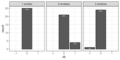
Figure 10: Histogram of hyperparameter estimation error $\Delta k$ across all setups (autocorrelated errors).

4 Real-World Data Experiments

In the second part of our experiments, we evaluate the performance of the Gaussian SWR model on two real-world examples. Both watersheds are located on the west coast of North America, with the first catchment representing the Koksilah River which is located in Cowichan, British Columbia, Canada. The second catchment represents the Smith River in Hiouchi, California, United States. The available dataset consists of 39 hydrological years for watershed 1 and 38 hydrological years for watershed 2. The Koksilah River has been investigated in previous works (Janssen et al., 2023).

4.1 Experimental Setup

Analogous to the simulation study, we use a training subset containing years 1 to 29 of the time series, followed by a test set covering 10 or 9 years, respectively (years 30 to 39 for watershed 1, and years 30 to 38 for watershed 2). The maximum number of windows is set to $k_{\max}=3$.

After an initial training run, the model residuals are evaluated for autocorrelations using the Durbin-Watson test. If autocorrelation is detected, the Cochrane-Orcutt procedure is applied. The Durbin-Watson test is applied again to verify that there is no evidence of correlation in the updated model.

4.2 Results

The Durbin-Watson test on the residuals from the model with untransformed data gives a p-value $<0.01$ in both cases, i.e. strong evidence against an independent-error model. In the case of watershed 1, an AR($2$) process with parameters $\varphi_{1}=0.46$ and $\varphi_{2}=0.13$ is indicated to model the autocorrelation, resulting in a Durbin-Watson p-value of $0.67$ after applying the Cochrane-Orcutt procedure. For watershed 2, an AR($1$) process with parameter $\varphi=0.64$ is sufficient to remove the autocorrelation, resulting in a p-value of $0.89$ after data transformation.

The estimated kernels for each watershed are illustrated in Fig. 11, and their parameters are estimated with uncertainty quantification in Table 4. Predictive performance scores ($R^{2}$, $KGE$, and RMSE) on the test set are shown in Table 5. Overall, the Gaussian SWR model achieves reasonably accurate prediction for both watersheds, e.g., $R^{2}$ scores of approximately 0.7 and 0.8, respectively.

Table 4: Parameter estimates after Cochrane-Orcutt transformation for real-world watersheds, with approximate standard errors.

watershed no	window no	$\beta_{i}$	$\delta_{i}$	$\sigma_{i}$
1	1	$0.45\pm 1e^{-2}$	$1.23\pm 2e^{-1}$	$3.01\pm 1e^{-1}$
	2	$0.40\pm 1e^{-2}$	$1.39\pm 4e^{-2}$	$0.08\pm 2e^{-2}$
2	1	$0.40\pm 6e^{-3}$	$0.00\pm 8e^{-2}$	$0.60\pm 6e^{-2}$
	2	$0.31\pm 8e^{-3}$	$1.84\pm 8e^{-3}$	$3.05\pm 1e^{-2}$
	3	$0.12\pm 5e^{-3}$	$11.68\pm 2e^{-1}$	$3.19\pm 7e^{-2}$

Table 5: Predictive performance metrics (on test set) after parameter estimation using Cochrane-Orcutt transformation for real-world watersheds. Evaluation metrics are computed on the original (untransformed) test set, as well as on the transformed test set.

watershed	$k$	metric
		$R^{2}$	KGE	RMSE
original data
1	2	0.70	0.77	3.38
2	3	0.79	0.86	4.32
transformed data
1	2	0.59	0.68	2.68
2	3	0.66	0.76	3.42

The Gaussian SWR model selects $k=2$ windows for watershed 1 and the maximum number of $k=3$ windows for watershed 2. Fig. 11 showa a clear dominance of the short-term history (window close to 0) in both cases. For the long-term history, the Gaussian SWR model selects two more distinguishable peaks for watershed 2, while all windows deployed for watershed 1 are centered at $\delta_{i}$ close to $0$, i.e. truncated. Thus, the combined kernel for watershed 1 resembles a truncated Student-t distribution with strong tails.

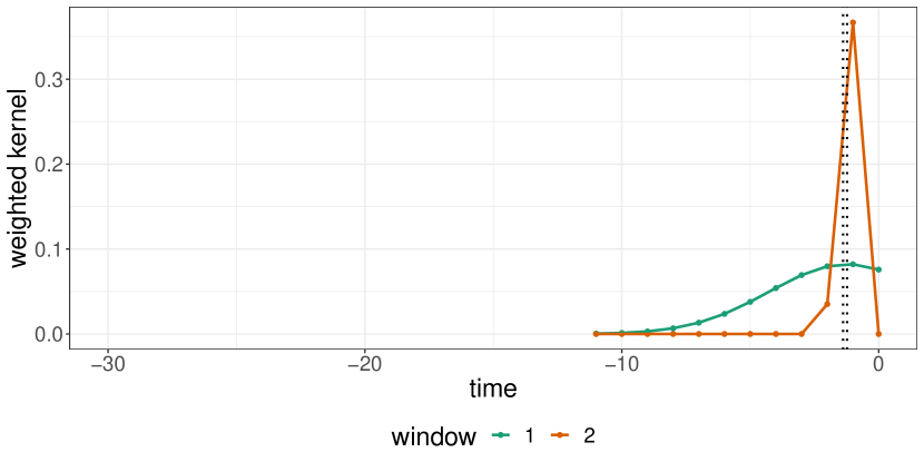
(a) Watershed 1.

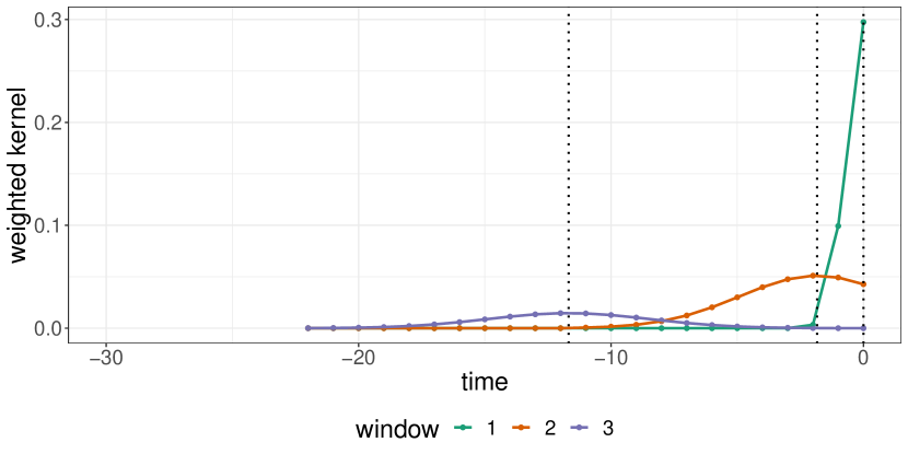
(b) Watershed 2.

Figure 11: Estimated scaled window kernels in real-world data experiments.

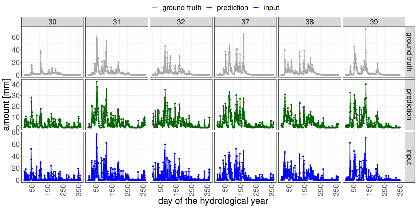
(a) Watershed 1.

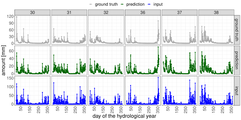
(b) Watershed 2.

Figure 12: Observed streamflow, predicted streamflow, and rainfall in the real-world experiments for six years of the test set

Fig. 12 compares the time series of predicted and observed waterflows for both watershed, along with the respective rainfall time series (all relating to untransformed data). To save space the plots restrict the time domain of the test set to the hydrological years 30–32 (years 1–3 of the test set) and hydrological years 37–39 or 36–38 (years 8–10 or 7–9) of the test set). Since the Gaussian SWR model acts as a smoothing operator on the input time series, the prediction time series is less spiked than the rainfall input and generally matches the shape of the ground truth well. However, time intervals with flat gauge values appear more noisy in the predictions, particularly for watershed 1.

4.3 Runtime Analysis

All experiments were performed on an Intel i7-8565U 1.8GHz CPU with 32GB RAM running Windows 11, where Algorithm 1 was implementated in R. The runtimes in Table 6 are averages over 5 independent model fits to account for variations in the computation time. In each run, the Gaussian SWR model is trained for one real-world watershed using the same experimental setup as in the real-world study; time to compute predictions is excluded. The maximum number of windows $k_{\max}$ is clearly important, but all runtimes are moderate.

Table 6: Runtimes of the Gaussian SWR model with $k_{\max}\in\{1,\dots,3\}$, averaged over 5 runs.

$k_{\max}$	runtime [s]
1	0.9
2	35.3
3	117.3

5 Discussion and Conclusion

Our experiments validated the Gaussian SWR model in a controlled experimental environment and real-world scenarios. Good predictive accuracy on a test set, as measured by $R^{2}$ for instance, was achieved throughout. The simulations demonstrated that achievable accuracy was dominated by the noise level, and rather independent of the number, position, size, and weighting of the ground truth windows. Moreover, multiple kernels were usually identifiable, with accurate parameter estimates. Thus, the proposed Gaussian SWR model has promising utility for hydrological inference.

Parameterizing the kernels as having Gaussian densities is easily extended to more flexible shapes, such as Student’s t, Gamma, or asymmetric generalized Laplace distributions. The latter two suggestions would enable long-tailed lag effects.

Relative to the more general DLM, the predictive performance of the Gaussian SWR model is comparable on the datasets used in our real-world experiments. The DLM implementation by Demirhan (2020) achieves test-set $R^{2}$ scores of 0.7 ($q=5$), 0.72 ($q=10$ and $q=20$) for watershed 1 and 0.79 ($q=5$), 0.8 ($q=10$), 0.81 ($q=20$) for watershed 2. Thus, the parametric assumption taken by Gaussian SWR, i.e. restricting the kernel shape to a mixture of Gaussians, does not significantly affect the predictive performance. However, the favorable parametrization employed by the Gaussian SWR model allows for straight-forward interpretations of the model parameters: the window position and size parameters are directly transferable to the concept of distinct flow paths in hydrology and deliver information on the expected lag of the runoff and its variance, respectively. Regression parameters $\bm{\beta}$ give indications of the relative importance of each flow path: while a dominant window with short lag typically models a strong short-term (overland) flow, well-distinguished windows with longer time lags indicate the presence of distinct long-term effects such as sub-surface or groundwater flows.

From a hydrological viewpoint, a major limitation of the Gaussian SWR model is that the kernels, particularly the parameters $\bm{\beta}$ and $\bm{\delta}$, do not change dynamically over the hydrologic year. The hydrologic year in many watersheds is characterized by drier and wetter periods, with distinct patterns in rainfall-runoff relationships. Related works by Janssen et al. (2023) on the same watershed 1 demonstrate that the predictive performance can be increased to approximately $R^{2}=0.8$ using a functional data analysis approach with dynamic regression weights and sparsity. Potentially, the Gaussian SWR model setup could be extended in future work to account for such dynamic parameters at the cost of a higher number of model parameters and a more complex training procedure, while keeping its highly interpretable ability to separate flow paths.

The presence of significant precipitation falling as snow will impact runoff dynamics in colder regions. As a consequence, runoff lags and magnitudes of the distinct flows paths may vary significantly over the year, which is not covered by linear constant-lag models. To overcome this issue for watersheds with significant snow to rainfall ratios, an extension of the proposed Gaussian SWR model to account for non-linearities would further be of interest. We consider this as another potential future extension of the proposed model.

From a machine learning viewpoint, the concept of convolving time series data with kernels is a well-established concept in artificial neural networks (ANNs), known as 1-dimensional convolution layers (Kiranyaz et al., 2021). In the neural network literature, the convolution of a window with the input time series acts as an integrated feature extraction step from the raw input, which is then mapped to the model output via a predictive model. In contrast to the neural network, our proposed method consists of a single layer (regression model) only, while ANNs allow for deeper architectures covering multiple layers of processing. Even though ANNs may therefore offer more flexibility and higher predictive model performance, the straight-forward interpretability of the regression parameters as weightings of the underlying flow paths would not hold when generalizing the model to a traditional multi-layer ANN. This ability could be devised and implemented, however, in impactful future works.

References

- Ahmad and Hossain [2020] S. K. Ahmad and F. Hossain. Maximizing energy production from hydropower dams using short-term weather forecasts. Renewable Energy, 146:1560–1577, 2020.
- Akaike [1974] H. Akaike. A new look at the statistical model identification. IEEE Transactions on Automatic Control, 19(6):716–723, Dec. 1974. doi:10.1109/tac.1974.1100705. URL https://doi.org/10.1109/tac.1974.1100705.
- Almon [1965] S. Almon. The distributed lag between capital appropriations and expenditures. Econometrica: Journal of the Econometric Society, pages 178–196, 1965.
- Baltagi [2022] B. H. Baltagi. Econometrics. Classroom Companion: Economics. Springer Nature, Cham, Switzerland, 6 edition, Jan. 2022.
- Botter et al. [2010] G. Botter, E. Bertuzzo, and A. Rinaldo. Transport in the hydrologic response: Travel time distributions, soil moisture dynamics, and the old water paradox. Water Resources Research, 46(3), Mar. 2010. doi:10.1029/2009wr008371. URL https://doi.org/10.1029/2009wr008371.
- Chen et al. [2018] Y.-H. Chen, B. Mukherjee, and V. J. Berrocal. Distributed lag interaction models with two pollutants. Journal of the Royal Statistical Society Series C: Applied Statistics, 68(1):79–97, July 2018. doi:10.1111/rssc.12297. URL https://doi.org/10.1111/rssc.12297.
- Cochrane and Orcutt [1949] D. Cochrane and G. H. Orcutt. Application of least squares regression to relationships containing auto-correlated error terms. Journal of the American Statistical Association, 44(245):32–61, Mar. 1949. doi:10.1080/01621459.1949.10483290. URL https://doi.org/10.1080/01621459.1949.10483290.
- Cornette et al. [2022] N. Cornette, C. Roques, A. Boisson, Q. Courtois, J. Marçais, J. Launay, G. Pajot, F. Habets, and J.-R. de Dreuzy. Hillslope-scale exploration of the relative contribution of base flow, seepage flow and overland flow to streamflow dynamics. Journal of Hydrology, 610:127992, 2022.
- Davtyan et al. [2020] A. Davtyan, A. Rodin, I. Muchnik, and A. Romashkin. Oil production forecast models based on sliding window regression. Journal of Petroleum Science and Engineering, 195:107916, Dec. 2020. doi:10.1016/j.petrol.2020.107916. URL https://doi.org/10.1016/j.petrol.2020.107916.
- Demirhan [2020] H. Demirhan. dLagM: An R package for distributed lag models and ARDL bounds testing. PLoS ONE, 15(2):e0228812, 2020. URL https://journals.plos.org/plosone/article?id=10.1371/journal.pone.0228812.
- Dunn et al. [2010] S. Dunn, C. Birkel, D. Tetzlaff, and C. Soulsby. Transit time distributions of a conceptual model: their characteristics and sensitivities. Hydrological Processes, 24(12):1719–1729, 2010.
- Eisner [1960] R. Eisner. A distributed lag investment function. Econometrica, Journal of the Econometric Society, pages 1–29, 1960.
- Everitt et al. [1981] B. S. Everitt, D. J. Hand, and B. Everitt. Finite Mixture Distributions. Monographs on Statistics & Applied Probability. Chapman and Hall, London, England, May 1981.
- Giani et al. [2021] G. Giani, M. A. Rico-Ramirez, and R. A. Woods. A practical, objective, and robust technique to directly estimate catchment response time. Water Resources Research, 57(2):e2020WR028201, 2021. doi:https://doi.org/10.1029/2020WR028201. URL https://agupubs.onlinelibrary.wiley.com/doi/abs/10.1029/2020WR028201. e2020WR028201 2020WR028201.
- Gilbert and Varadhan [2019] P. Gilbert and R. Varadhan. numDeriv: Accurate Numerical Derivatives, 2019. URL https://CRAN.R-project.org/package=numDeriv. R package version 2016.8-1.1.
- Griliches [1967] Z. Griliches. Distributed lags: A survey. Econometrica: journal of the Econometric Society, pages 16–49, 1967.
- Gupta et al. [2009] H. V. Gupta, H. Kling, K. K. Yilmaz, and G. F. Martinez. Decomposition of the mean squared error and NSE performance criteria: Implications for improving hydrological modelling. Journal of Hydrology, 377(1-2):80–91, Oct. 2009. doi:10.1016/j.jhydrol.2009.08.003. URL https://doi.org/10.1016/j.jhydrol.2009.08.003.
- Hare et al. [2021] D. K. Hare, A. M. Helton, Z. C. Johnson, J. W. Lane, and M. A. Briggs. Continental-scale analysis of shallow and deep groundwater contributions to streams. Nature Communications, 12(1), Mar. 2021. doi:10.1038/s41467-021-21651-0. URL https://doi.org/10.1038/s41467-021-21651-0.
- Harman et al. [2011] C. Harman, P. Troch, and M. Sivapalan. Functional model of water balance variability at the catchment scale: 2. elasticity of fast and slow runoff components to precipitation change in the continental united states. Water Resources Research, 47(2), 2011.
- Hyndman and Athanasopoulos [2021] R. J. Hyndman and G. Athanasopoulos. Forecasting. OTexts, Australia, 3 edition, May 2021.
- Janssen et al. [2021] J. Janssen, V. Radić, and A. Ameli. Assessment of future risks of seasonal municipal water shortages across north america. Frontiers in Earth Science, 9:730631, 2021.
- Janssen et al. [2023] J. Janssen, S. Meng, A. Haris, S. Schrunner, J. Cao, W. J. Welch, N. Kunz, and A. A. Ameli. Learning from limited temporal data: Dynamically sparse historical functional linear models with applications to earth science. arXiv preprint arXiv:2303.06501, 2023.
- Johnson [2021] S. G. Johnson. The NLopt nonlinear-optimization package, 2021. URL http://github.com/stevengj/nlopt. v2.7.1.
- Kannan et al. [2007] N. Kannan, S. White, F. Worrall, and M. Whelan. Hydrological modelling of a small catchment using swat-2000–ensuring correct flow partitioning for contaminant modelling. Journal of Hydrology, 334(1-2):64–72, 2007.
- Khan et al. [2019] I. A. Khan, A. Akber, and Y. Xu. Sliding window regression based short-term load forecasting of a multi-area power system. In 2019 IEEE Canadian Conference of Electrical and Computer Engineering (CCECE). IEEE, May 2019. doi:10.1109/ccece.2019.8861915. URL https://doi.org/10.1109/ccece.2019.8861915.
- Kiranyaz et al. [2021] S. Kiranyaz, O. Avci, O. Abdeljaber, T. Ince, M. Gabbouj, and D. J. Inman. 1d convolutional neural networks and applications: A survey. Mechanical Systems and Signal Processing, 151:107398, 2021. ISSN 0888-3270. doi:https://doi.org/10.1016/j.ymssp.2020.107398. URL https://www.sciencedirect.com/science/article/pii/S0888327020307846.
- Kuhn and Johnson [2019] M. Kuhn and K. Johnson. Applied Predictive Modeling. Springer New York, 2019. ISBN 9781493979363.
- Mauricio Zambrano-Bigiarini [2020] Mauricio Zambrano-Bigiarini. hydroGOF: Goodness-of-fit functions for comparison of simulated and observed hydrological time series, 2020. URL https://github.com/hzambran/hydroGOF. R package version 0.4-0.
- McMillan [2020] H. McMillan. Linking hydrologic signatures to hydrologic processes: A review. Hydrological Processes, 34(6):1393–1409, 2020.
- Nash and Sutcliffe [1970] J. Nash and J. Sutcliffe. River flow forecasting through conceptual models part i — a discussion of principles. Journal of Hydrology, 10(3):282–290, Apr. 1970. doi:10.1016/0022-1694(70)90255-6. URL https://doi.org/10.1016/0022-1694(70)90255-6.
- Nejadhashemi et al. [2009] A. P. Nejadhashemi, A. Shirmohammadi, J. M. Sheridan, H. J. Montas, and K. R. Mankin. Case study: evaluation of streamflow partitioning methods. Journal of irrigation and drainage engineering, 135(6):791–801, 2009.
- Peng et al. [2009] R. D. Peng, F. Dominici, and L. J. Welty. A bayesian hierarchical distributed lag model for estimating the time course of risk of hospitalization associated with particulate matter air pollution. Journal of the Royal Statistical Society: Series C (Applied Statistics), 58(1):3–24, Feb. 2009. doi:10.1111/j.1467-9876.2008.00640.x. URL https://doi.org/10.1111/j.1467-9876.2008.00640.x.
- Powell [2009] M. J. Powell. The bobyqa algorithm for bound constrained optimization without derivatives. Cambridge NA Report NA2009/06, University of Cambridge, Cambridge, 26, 2009.
- R Core Team [2022] R Core Team. R: A Language and Environment for Statistical Computing. R Foundation for Statistical Computing, Vienna, Austria, 2022. URL https://www.R-project.org/.
- Roksvg et al. [2021] T. Roksvg, I. Steinsland, and K. Engeland. A two-field geostatistical model combining point and areal observations—a case study of annual runoff predictions in the voss area. Journal of the Royal Statistical Society Series C: Applied Statistics, 70(4):934–960, Aug. 2021. doi:10.1111/rssc.12492. URL https://doi.org/10.1111/rssc.12492.
- Rushworth [2018] A. Rushworth. Bayesian distributed lag models, 2018.
- Rushworth et al. [2013] A. M. Rushworth, A. W. Bowman, M. J. Brewer, and S. J. Langan. Distributed lag models for hydrological data. Biometrics, 69(2):537–544, 2013.
- Sawicz et al. [2014] K. Sawicz, C. Kelleher, T. Wagener, P. Troch, M. Sivapalan, and G. Carrillo. Characterizing hydrologic change through catchment classification. Hydrology and Earth System Sciences, 18(1):273–285, 2014.
- Schwarz [1978] G. Schwarz. Estimating the dimension of a model. The Annals of Statistics, 6(2), Mar. 1978. doi:10.1214/aos/1176344136. URL https://doi.org/10.1214/aos/1176344136.
- Tang et al. [2009] Q. Tang, E. Rosenberg, and D. Lettenmaier. Use of satellite data to assess the impacts of irrigation withdrawals on upper klamath lake, oregon. Hydrology and Earth System Sciences, 13(5):617–627, 2009.
- Warren et al. [2020] J. L. Warren, T. J. Luben, and H. H. Chang. A spatially varying distributed lag model with application to an air pollution and term low birth weight study. Journal of the Royal Statistical Society Series C: Applied Statistics, 69(3):681–696, Mar. 2020. doi:10.1111/rssc.12407. URL https://doi.org/10.1111/rssc.12407.
- Young [2006] P. C. Young. Rainfall-Runoff Modeling: Transfer Function Models, chapter 128. John Wiley & Sons, Ltd, 2006. ISBN 9780470848944. doi:https://doi.org/10.1002/0470848944.hsa141a. URL https://onlinelibrary.wiley.com/doi/abs/10.1002/0470848944.hsa141a.
- Zalewski et al. [2000] M. Zalewski et al. Ecohydrology—the scientific background to use ecosystem properties as management tools toward sustainability of water resources. Ecological engineering, 16(1):1–8, 2000.