Fast Variational Block-Sparse Bayesian Learning

Abstract

We present a fast update rule for variational block-sparse Bayesian learning (SBL) methods. Based on a variational Bayesian approximation, we show that iterative updates of probability density functions (PDFs) of the prior precisions and weights can be expressed as a nonlinear first-order recurrence from one estimate of the parameters of the proxy PDFs to the next. In particular, for commonly used prior PDFs such as Jeffrey’s prior, the recurrence relation turns out to be a strictly increasing rational function. This property is the basis for two important analytical results. First, the determination of fixed points by solving for the roots of a polynomial. Second, the determination of the limit of the prior precision after an infinite sequence of update steps. These results are combined into a simplified single-step check for convergence/divergence of each prior precision. Consequently, our proposed criterion significantly reduces the computational complexity of the variational block-SBL algorithm, leading to a remarkable two orders of magnitude improvement in convergence speed shown by simulations. Moreover, the criterion provides valuable insights into the sparsity of the estimators obtained by different prior choices.

I Introduction

Sparse signal models have gained widespread adoption over the last 20 years through the advent of compressed sensing [1]. Generally, the aim of sparse signal reconstruction algorithms is to reconstruct a signal based on a large dictionary matrix as a weighted linear combination of only a few (non-zero) entries of the dictionary. One approach to solve this problem is sparse Bayesian learning (SBL). SBL uses the normal variance mixture model [2] which models the prior precision, i.e., inverse variance, of each weight as a hyperparameter. These hyperparameters are estimated from the data [3, 4, 5, 6]. Extensions to block-sparse signal models have been developed, where the weights are grouped into blocks, with only a small number of blocks differing from the zero vector [7, 8, 9, 10].

A major shortcoming of the SBL framework is the slow convergence rate of the hyperparameter estimation. However, this problem was alleviated by the introduction of a fast method to maximize the marginal likelihood [4, 5]. In [11], this fast method for maximizing the marginalized likelihood is extended to multiple measurement vectors, which is closely related to block sparsity. Additionally, [11] shows that the hyperparameters can be analytically determined by solving for the roots of a polynomial. However, solving the polynomial with a considerable order was not computationally efficient for the application outlined in [11]. Therefore, an iterative maximization procedure was utilized. In [12], the authors introduced an adaption of the fast marginal likelihood maximization method from [11] tailored to block-sparse models.

Alternatively, SBL can be derived within a variational Bayesian framework [13, 14, 15, 16]. In this framework, (approximate) posterior distributions of the parameters are estimated by maximizing the evidence lower bound (ELBO) [17] [18, Ch. 10]. Since posterior probability density functions (PDFs) are estimated instead of point estimates only, the variational approach provides a more complete characterization of the parameters of interest. Furthermore, different hyperpriors, i.e. prior PDFs on the hyperparameters, lead to different estimators. By choosing a parameterized PDF as hyperprior, which encompasses many commonly used hyperpriors as special cases of its parameters, we compare different variants of SBL within the same framework [15, 19]. A fast update rule for the hyperparameters is of critical importance for this analysis. For non-blocked variational SBL such a fast update rule is proposed in [13] by identifying the fixed points of a recurrent sequence of variational updates. However, extending the solution in [13] to block-sparse models is not trivial.

Contribution

The main contribution of this work is the expansion of the variational SBL method, as introduced in [13], to block-sparse models. In particular, we extend and generalize [13, Theorem 1] to block-sparse models. Since [13, Theorem 1] merely provides the condition for one (locally stable) fixed point to be existent, it cannot be used in it’s original form. We show (i) that for block-sparse models potentially multiple such fixed points exists and (ii) that the fixed points of the variational update sequence for block-sparse models can be found as the roots of a polynomial. To make the fast update rule [13] applicable to block sparse models, we need to identify to which fixed point the variational update sequence converges.

Our new theorem, as stated in Theorem 1, enables the calculation of the limit of the variational update sequence. I.e., it allows to determine to which fixed point the variational update sequence converges, which is crucial to the block-sparse fast update rule. Noted that [13, Theorem 1] is regarded as a special case of Theorem 1, where each block consists of only a single component.

Based on Theorem 1, we derive a fast variational block-sparse SBL algorithm with the following advantages.

• The runtime of our algorithm is up to two orders of magnitude smaller than that of similar block-SBL algorithms [9], while simultaneously achieving a better performance in terms of the normalized mean squared error (NMSE) and the probability of correctly recovering the support.

• We can obtain many commonly used hyperprior distributions by modeling the hyperprior as a generalized inverse Gaussian distribution. Thus, the estimators obtained by using different hyperpriors can be analyzed and compared directly using our solution.

• We show that for a certain parameterization of the generalized inverse Gaussian distribution, our proposed method is equivalent to the method of fast marginal likelihood maximization for block-SBL [12]. However, since different parameter settings of the hyperprior lead to different estimators our method is more general.

• We apply our proposed block-SBL to a direction of arrival (DOA) estimation problem and show the benefits compared to the multi-snapshot SBL-based DOA estimation algorithm in [20].

Since a fast block-SBL was already presented by [12], we would like to highlight the similarities and differences between our approach and [12]. While the approach of [12] is based on maximizing the marginalized likelihood similar to [5], we address the issue through the framework of variational Bayesian inference. The variational Bayesian approach allows to consider and analyze different hyperpriors and, thus, different estimators whereas [12] is shown to be equivalent to a special case of our parameterized hyperprior. Another advantage of the variational Bayesian approach is that it can be easily extended to include the estimation of additional parameters such as using a parametrized (infinite) dictionary matrix similar to [14, 21]. Note that the variational Bayesian approach can be easily incorporated into message passing algorithms, such as belief propagation [22]. This integration can be utilized in joint channel estimation and decoding of MIMO communication systems [23, 24, 25].

II Overview of the Block-Sparse SBL Framework

II-A System Model

We aim to estimate the weights $\bm{x}$ in the linear model

$$\bm{y}=\bm{\Phi}\bm{x}+\bm{v}$$ (1)

where $\bm{y}$ is the observed signal vector of length $N$, $\bm{\Phi}$ is an $N\times M$ dictionary matrix and $\bm{v}$ is additive white Gaussian noise (AWGN) with precision $\lambda\in\mathbb{R}_{\geq 0}$. Thus, the likelihood function is given by the PDF $p(\bm{y}|\bm{x},\lambda)=\mathcal{N}(\bm{y};\bm{\Phi}\bm{x},\lambda^{-1}\bm{I})$. To allow for both a real-valued and complex-valued signal model, we use a parameterized likelihood function.

We assume that $\bm{x}$ is block-sparse, meaning that the $M$-length vector $\bm{x}$ is partitioned into $K$ blocks $\bm{x}_{i}$ of known size $d_{i}$ each, e.g.

$$\bm{x}=[\underbrace{x_{1}\hskip 2.84526ptx_{2}\,\cdots\,x_{d_{1}}}_{\bm{x}_{1}^{\text{T}}}\,\cdots\,\,\cdots\,\underbrace{x_{M-d_{K}+1}\,\cdots\,x_{M}}_{\bm{x}_{K}^{\text{T}}}]^{\text{T}}$$ (2)

for which $\bm{x}_{i}=\bm{0}$ for all except a few blocks $i$. Note that we can transform any problem with joint sparsity in groups of non-neighboring weights to the blocked form illustrated in (2) by rearranging the columns of the dictionary matrix $\bm{\Phi}$ and the entries of $\bm{x}$. Furthermore, consider the multiple measurement vector (MMV) signal model

$$\bm{Y}=\bm{\Psi}\bm{X}+\bm{V}$$ (3)

where $\bm{Y}=[\bm{y}_{1}\hskip 2.84526pt\bm{y}_{2}\,\cdots\,\bm{y}_{J}]$ is a matrix of $J$ measurement vectors $\bm{y}_{j}$, $\bm{\Psi}$ is some dictionary matrix with corresponding weights $\bm{X}$, and $\bm{V}$ is a matrix of additive noise. A common assumption is that the sparsity profile is the same for each column in $\bm{X}$, i.e. that all elements in each row of $\bm{X}$ are either jointly zero or nonzero. Let $\bm{y}=\text{vec}(\bm{Y}^{\text{T}})$, $\bm{x}=\text{vec}(\bm{X}^{\text{T}})$, and $\bm{v}=\text{vec}(\bm{V}^{\text{T}})$, where $\text{vec}(\bm{X})$ denote the operation of stacking all the columns of the $N\times M$ matrix $\bm{X}$ into an $NM\times 1$ column vector. Furthermore, let $\bm{\Phi}=\bm{\Psi}\otimes\bm{I}_{J}$ be the Kronecker product of $\bm{\Psi}$ with the $J\times J$ identity matrix $\bm{I}_{J}$, finding the row-sparse matrix $\bm{X}$ in (3) is equivalent to finding the block-sparse weight vector $\bm{x}$ in (1).

The block-sparse or MMV problem has many applications. E.g. the estimation of block-sparse channels in multiple-input multiple-output communication systems [23, 24] or DOA estimation using the MMV model [20]. We provide an example of how to apply the system model in (3) to MMV-DOA estimation in Section VII.

II-B SBL Probabilistic Model

SBL solves the sparse signal reconstruction task of (1) through the mechanism of automatic relevance detection [3]. We use a normal variance mixture model [2] and model the prior for each block $\bm{x}_{i}$ as a zero-mean Gaussian PDF

$$p(\bm{x}_{i}|\gamma_{i})=\mathcal{N}\big{(}\bm{x}_{i};\bm{0},(\gamma_{i}\bm{B}_{i})^{-1}\big{)}\,.$$ (4)

with precision matrix $\gamma_{i}\bm{B}_{i}$, where $\bm{B}_{i}$ is a known matrix characterizing the intra-block correlation and $\gamma_{i}\in\mathbb{R}_{\geq 0}$ is a hyperparameter which scales the prior precision matrix of each block [4, 5, 6]. The different blocks of weights $\bm{x}_{i}$ are assumed independent, i.e. $p(\bm{x}|\bm{\gamma})=\prod_{i=1}^{K}p(\bm{x}_{i}|\gamma_{i})$, denoting $\bm{\gamma}=[\gamma_{1}\hskip 2.84526pt\hskip 0.85358pt\gamma_{2}\,\cdots\,\gamma_{K}]^{\text{T}}$. By estimating $\bm{\gamma}$ from the data, the relevance of each block is automatically determined. For many blocks $i$ the estimate of $\gamma_{i}$ diverges. These blocks are effectively removed from the model as the corresponding estimate of $\bm{x}_{i}$ approaches $\bm{0}$.

To perform (approximate) Bayesian inference, we place independent hyperprior PDFs $p(\bm{\gamma})=\prod_{i=1}^{K}p(\gamma_{i})$ over the unknown hyperparameters $\gamma_{i}$. Given $p(\bm{x}|\bm{\gamma})$ and $p(\bm{\gamma})$, the prior on the weights is obtained as

$$p(\bm{x})=\int p(\bm{x}|\bm{\gamma})p(\bm{\gamma})\,\text{d}\bm{\gamma}.$$ (5)

Hence, by specifying different hyperprior PDFs $p(\bm{\gamma})$, we obtain different priors $p(\bm{x})$ and, thus, different estimators. Commonly used PDFs for $p(\gamma_{i})$ include the Gamma and inverse Gamma PDFs as well as Jeffrey’s prior $p(\gamma_{i})\propto\gamma_{i}^{-1}$ [13, 19, 15]. The generalized inverse Gaussian distribution [26]

$$p(\gamma_{i};a_{i},b_{i},c_{i})=\frac{\big{(}\frac{a_{i}}{b_{i}}\big{)}^{\frac{c_{i}}{2}}\gamma_{i}^{c_{i}-1}}{2K_{c_{i}}(\sqrt{a_{i}b_{i}})}\exp\big{\{}-\frac{1}{2}(a_{i}\gamma_{i}+b_{i}\gamma_{i}^{-1})\big{\}}$$ (6)

where $K_{c}(\cdot)$ denotes the modified Bessel function of the second kind, includes the aforementioned PDFs as special cases of the parameters $a_{i}$, $b_{i}$ and $c_{i}$ as shown in the first and second column of Table I. Moreover, this choice of prior for $p(\bm{\gamma})$ is conjugate for Gaussian $p(\bm{x}|\bm{\gamma})$, which allows to solve the variational updates analytically [15]. Therefore, we consider a generalized inverse Gaussian distribution as hyperprior $p(\gamma_{i})$ throughout this work.

To complete the Bayesian model, we also need a prior PDF for the noise precision $\lambda$. We use a Gamma PDF with shape $\epsilon$ and rate $\eta$

$$p(\lambda;\epsilon,\eta)=\frac{\eta^{\epsilon}}{\Gamma(\epsilon)}\lambda^{\epsilon-1}\exp\{-\eta\lambda\}$$ (7)

where $\Gamma(\cdot)$ denotes the Gamma function, since this is a conjugate prior for the precision of a Gaussian distribution.

II-C Variational Bayesian Inference

We apply variational inference [17] [18, Ch. 10] to approximate the posterior PDF of the parameters $\bm{x}$, $\bm{\gamma}$ and $\lambda$

$$p(\bm{x},\bm{\gamma},\lambda|\bm{y})\propto p(\bm{y}|\bm{x},\lambda)p(\bm{x}|\bm{\gamma})p(\bm{\gamma})p(\lambda)$$ (8)

with a simpler, factorized distribution $q(\bm{x},\bm{\gamma},\lambda)$. Specifically, we apply the structured mean-field assumption $q(\bm{x},\bm{\gamma},\lambda)=q_{\bm{x}}(\bm{x})q_{\lambda}(\lambda)\prod_{i=1}^{K}q_{\gamma_{i}}(\gamma_{i})$ to approximate the posterior PDF as

$$p(\bm{x},\bm{\gamma},\lambda|\bm{y})\approx q_{\bm{x}}(\bm{x})q_{\lambda}(\lambda)\prod_{i=1}^{K}q_{\gamma_{i}}(\gamma_{i}).$$ (9)

Each factor $q_{j}\in\mathcal{Q}=\{q_{\bm{x}},\,q_{\lambda},\,q_{\gamma_{1}},\,q_{\gamma_{2}},\,\cdots,\,q_{\gamma_{K}}\}$ of $q(\bm{x},\bm{\gamma},\lambda)$ in (9) is found by maximizing the ELBO

$$\mathcal{L}(q)=\bigg{<}\ln\frac{p(\bm{x},\bm{\gamma},\lambda|\bm{y})}{q(\bm{x},\bm{\gamma},\lambda)}\bigg{>}_{q(\bm{x},\bm{\gamma},\lambda)}$$ (10)

where $\big{<}f(\cdot)\big{>}_{q(\cdot)}$ denotes the expectation of the function $f(\cdot)$ depending on random variables distributed with PDF $q(\cdot)$. Maximizing the ELBO (10) is equivalent to minimizing the Kullback-Leibler (KL)-divergence between the true posterior and the approximation $q$ [17] [18, Ch. 10]. The factors $q_{j}\in\mathcal{Q}$ are updated iteratively using

$$q_{j}\propto\exp\big{\{}\big{<}\ln p(\bm{x},\bm{\gamma},\lambda|\bm{y})\big{>}_{q_{\bar{j}}}\big{\}}$$ (11)

while keeping the remaining factors $q_{l}\in\mathcal{Q}\backslash\{q_{j}\}$ fixed. We denote $q_{\bar{j}}=\prod_{q_{l}\in\mathcal{Q}\backslash\{q_{j}\}}q_{l}$ as the product of all factors in $\mathcal{Q}$ except for $q_{j}$. Inserting the posterior (8) into (11), we obtain

$$q_{\bm{x}}(\bm{x})=\mathcal{N}(\bm{x};\hat{\bm{x}},\,\hat{\bm{\Sigma}})$$ (12)

as a Gaussian PDF with mean

$$\hat{\bm{x}} =\hat{\lambda}\hat{\bm{\Sigma}}\bm{\Phi}^{\text{H}}\bm{y}$$ (13)

and covariance matrix

$$\hat{\bm{\Sigma}}=(\hat{\lambda}\bm{\Phi}^{\text{H}}\bm{\Phi}+\bm{B}_{\bm{\gamma}})^{-1}$$ (14)

where $\hat{\lambda}=\big{<}\lambda\big{>}_{q_{\lambda}}$ is the current estimate of the noise precision, $\bm{B}_{\bm{\gamma}}$ is a block-diagonal matrix with the principal diagonal blocks $\hat{\gamma}_{i}\bm{B}_{i}$, and $\hat{\gamma}_{i}=\big{<}\gamma_{i}\big{>}_{q_{\gamma_{i}}}$ is the mean of $q_{\gamma_{i}}$ [15]. Similarly, by inserting (8) into (11) we get

$$q_{\gamma_{i}}(\gamma_{i})\propto\gamma_{i}^{\hat{c}_{i}-1}\exp\big{\{}-\frac{1}{2}(\hat{a}_{i}\gamma_{i}+b_{i}\gamma_{i}^{-1})\big{\}}$$ (15)

for $i\in\{1,\,2,\,\cdots,\,K\}$. I.e. $q_{\gamma_{i}}$ is the PDF of a generalized inverse Gaussians distribution with parameters $\hat{a}_{i}=2\rho\big{<}\bm{x}_{i}^{\text{H}}\bm{B}_{i}\bm{x}_{i}\big{>}_{q_{\bm{x}}}+a_{i}$, $b_{i}$ and $\hat{c}_{i}=c_{i}+\rho d_{i}$ [15]. For the update of the other factors in $\mathcal{Q}$ only the expectations $\hat{\gamma}_{i}=\big{<}\gamma_{i}\big{>}_{q_{\gamma_{i}}}$ are required, which can be computed from $\hat{a}_{i}$, $b_{i}$, and $\hat{c}_{i}$ as [15, 26]

$$\hat{\gamma}_{i}=\big{<}\gamma_{i}\big{>}_{q_{\gamma_{i}}} =\frac{\sqrt{b_{i}}}{\sqrt{\hat{a}_{i}}}\frac{K_{\hat{c}_{i}+1}\big{(}\sqrt{\hat{a}_{i}\hskip 0.85358ptb_{i}}\big{)}}{K_{\hat{c}_{i}}\big{(}\sqrt{\hat{a}_{i}\hskip 0.85358ptb_{i}}\big{)}}\hskip 0.85358pt.$$ (16)

Simplified expressions of the update equation (16) for different selections of the parameters settings $a_{i}$, $b_{i}$ and $c_{i}$ are listed in the third column of Table I. Note, that if Jeffery’s prior is used, the simplified form $\hat{\gamma}_{i}=d_{i}/\big{<}\bm{x}_{i}^{\text{H}}\bm{B}_{i}\bm{x}_{i}\big{>}_{q_{\bm{x}}}$ of (16) given in the last row of Table I is equivalent to the update rule [9, Eq. (4)] obtained by applying the expectation-maximization (EM)-algorithm. Hence, the presented fast solution can also be applied to [9] and similar EM-based block-SBL algorithms.

Finally, by inserting (8) into (11) we obtain

$$q_{\lambda}(\lambda)\propto\lambda^{\hat{\epsilon}-1}\exp\{-\hat{\eta}\lambda\}$$ (17)

i.e. a Gamma PDF with shape $\hat{\epsilon}=\rho N+\epsilon$ and rate $\hat{\eta}=\rho\big{(}\|\bm{y}-\bm{\Phi}\hat{\bm{x}}\|^{2}+\text{tr}(\bm{\Phi}^{\text{H}}\bm{\Phi}\hat{\bm{\Sigma}})\big{)}+\eta$. The expectation $\hat{\lambda}$ of $q_{\lambda}$ is

$$\hat{\lambda}=\big{<}\lambda\big{>}_{q_{\lambda}}=\frac{\rho N+\epsilon}{\rho\big{(}\|\bm{y}-\bm{\Phi}\hat{\bm{x}}\|^{2}+\text{tr}(\bm{\Phi}^{\text{H}}\bm{\Phi}\hat{\bm{\Sigma}})\big{)}+\eta}\hskip 0.85358pt.$$ (18)

TABLE I: Fast update rules of $\hat{\gamma}_{i}$ for different parametrizations of $p(\gamma_{i})$, expanding on [15, Table 1]

Hyperprior Shape	Hyperprior Parameters	Update of $\hat{\gamma}_{i}$	$f_{i}(\hat{\gamma}_{i})$	Fast Update Polynomial $G_{i}(\hat{\gamma}_{i})$	Sparse
Generalized inverse Gaussian	$a_{i}>0$, $b_{i}>0$, $c_{i}\in\mathbb{R}$	$\sqrt{\frac{b_{i}}{\hat{a}_{i}}}\frac{K_{\hat{c}_{i}+1}\big{(}\sqrt{\hat{a}_{i}\hskip 0.85358ptb_{i}}\big{)}}{K_{\hat{c}_{i}}\big{(}\sqrt{\hat{a}_{i}\hskip 0.85358ptb_{i}}\big{)}}$	-	-	-
Inverse Gamma	$a_{i}\rightarrow 0$, $b_{i}>0$, $c_{i}=-\rho d_{i}-\frac{1}{2}$	$\sqrt{\frac{b_{i}}{2\rho\big{<}\bm{x}_{i}^{\text{H}}\bm{B}_{i}\bm{x}_{i}\big{>}_{q_{\bm{x}}}}}$	$\sqrt{\frac{b_{i}A_{i}(\hat{\gamma}_{i})}{2\rho B_{i}(\hat{\gamma}_{i})}}$	$b_{i}A_{i}(\hat{\gamma}_{i})-2\rho\hat{\gamma}_{i}^{2}B_{i}(\hat{\gamma}_{i})$	No
Gamma	$a_{i}>0$, $b_{i}\rightarrow 0$, $c_{i}>0$	$\frac{c_{i}+\rho d_{i}}{\rho\big{<}\bm{x}_{i}^{\text{H}}\bm{B}_{i}\bm{x}_{i}\big{>}_{q_{\bm{x}}}+\frac{a_{i}}{2}}$	$\frac{c_{i}+\rho d_{i}}{\rho\frac{B_{i}(\hat{\gamma}_{i})}{A_{i}(\hat{\gamma}_{i})}+\frac{a_{i}}{2}}$	$(c_{i}+\rho d_{i})A_{i}(\hat{\gamma}_{i})-\hat{\gamma}_{i}\big{(}\rho B_{i}(\hat{\gamma}_{i})+\frac{a_{i}}{2}A_{i}(\hat{\gamma}_{i})\big{)}$	No
Scaled Jeffrey’s $p(\gamma_{i})\propto\gamma_{i}^{-1+c_{i}}$	$a_{i}\rightarrow 0$, $b_{i}\rightarrow 0$, $c_{i}>-\rho d_{i}$	$\frac{c_{i}+\rho d_{i}}{\rho\big{<}\bm{x}_{i}^{\text{H}}\bm{B}_{i}\bm{x}_{i}\big{>}_{q_{\bm{x}}}}$	$\frac{c_{i}+\rho d_{i}}{\rho\frac{B_{i}(\hat{\gamma}_{i})}{A_{i}(\hat{\gamma}_{i})}}$	$(c_{i}+\rho d_{i})A_{i}(\hat{\gamma}_{i})-\rho\hat{\gamma}_{i}B_{i}(\hat{\gamma}_{i})$	Yes if $c_{i}>0$
Jeffrey’s $p(\gamma_{i})\propto\gamma_{i}^{-1}$	$a_{i}\rightarrow 0$, $b_{i}\rightarrow 0$, $c_{i}\rightarrow 0$	$\frac{d_{i}}{\big{<}\bm{x}_{i}^{\text{H}}\bm{B}_{i}\bm{x}_{i}\big{>}_{q_{\bm{x}}}}$	$\frac{d_{i}A_{i}(\hat{\gamma}_{i})}{B_{i}(\hat{\gamma}_{i})}$	$d_{i}A_{i}(\hat{\gamma}_{i})-\hat{\gamma}_{i}B_{i}(\hat{\gamma}_{i})$	Yes

• Note that our model is slightly different from the one used in [15]. The hyperparameters $\gamma_{i}$ correspond to $z_{i}^{-1}$ in [15]. This reparametrization results in a swap of the hyperprior parameters $a_{i}$ and $b_{i}$, and a change in the sign of $c_{i}$ compared to [15, Table 1]. Furthermore, the Gamma hyperprior PDF corresponds to the inverse Gamma mixing distribution of [15, Table 1] and vice versa.

III Variational Fast Solution

III-A Derivation of the Fast Solution

In the variational Bayesian framework, a solution is typically obtained by iterating the update equations (13), (14), (16) and (18) until convergence. However, the convergence of the hyperparameters $\hat{\gamma}_{i}$ can be slow due to the cyclic dependency of $\hat{\gamma}_{i}$ on $\hat{\bm{x}}$ and $\hat{\bm{\Sigma}}$ and vice versa. To accelerate convergence, we analyse how the parameters $\hat{\gamma}_{i}$ of the distribution $q_{\gamma_{i}}$ of a single hyperprior behave if updates of $q_{\bm{x}}$ and $q_{\gamma_{i}}$ are repeated ad infinitum. Following the approach of [13], we consider the sequence of estimates $\{\hat{\gamma}_{i}^{[n]}\}_{n=1}^{\infty}$ obtained by repeated cycles of updating $q_{\bm{x}}$ followed by updating $q_{\gamma_{i}}$. For specific parameter settings $a_{i}$, $b_{i}$ and $c_{i}$, each element of the sequence can be calculated by the simplified version of (16) listed in the third column of Table I. We are interested in knowing if the sequence converges and, if it does converge, in its limit.

Note, that the expression $h_{i}(\hat{\gamma}_{i}):=\big{<}\bm{x}_{i}^{\text{H}}\bm{B}_{i}\bm{x}_{i}\big{>}_{q_{\bm{x}}}$ in the update equations for $\hat{\gamma}_{i}$ given in the third column of Table I is a function of the previous estimate of $\hat{\gamma}_{i}$ trough (13) and (14). Hence, the sequence of estimates $\hat{\gamma}_{i}^{[n]}$ obtained by repeatedly updating $q_{\bm{x}}$ followed by $q_{{\gamma}_{i}}$ can be viewed as generated by a first-order recurrence $f_{i}$ : $\mathbb{R}_{\geq 0}\rightarrow\mathbb{R}_{\geq 0}$ which maps from one estimate in the sequence to the next as $\hat{\gamma}_{i}^{[n+1]}=f_{i}(\hat{\gamma}_{i}^{[n]})$. If the update sequence converges, the limit must be a fixed point

$$\hat{\gamma}_{i}^{\ast}\in\mathcal{G}_{i}=\{\hat{\gamma}_{i}\in\mathbb{R}_{\geq 0}:f_{i}(\hat{\gamma}_{i})-\hat{\gamma}_{i}=0\}$$ (19)

of this recurrent relation.

As we show in Section III-B, the function $h_{i}(\hat{\gamma}_{i})$ can be expressed as a rational function

$$h_{i}(\hat{\gamma}_{i})=\big{<}\bm{x}_{i}^{\text{H}}\bm{B}_{i}\bm{x}_{i}\big{>}_{q_{\bm{x}}}=\frac{B_{i}(\hat{\gamma}_{i})}{A_{i}(\hat{\gamma}_{i})}$$ (20)

where $A_{i}(\hat{\gamma}_{i})$ and $B_{i}(\hat{\gamma}_{i})$ are two polynomials in $\hat{\gamma}_{i}$.

We insert the simplified update equations $f_{i}$, given in the fourth column of Table I, and (20) into the fixed point equation $f_{i}(\hat{\gamma}_{i})-\hat{\gamma}_{i}=0$ to find the fixed points $\hat{\gamma}_{i}^{\ast}$ as solutions to the polynomial equation $G_{i}(\hat{\gamma}_{i})=0$ after a few algebraic manipulations. Thus, the sets of fixed points $\mathcal{G}_{i}$ can be obtained as

$$\mathcal{G}_{i} =\{\hat{\gamma}_{i}\in\mathbb{R}_{\geq 0}:G_{i}(\hat{\gamma}_{i})=0\}\,.$$ (21)

Different polynomials $G_{i}(\hat{\gamma}_{i})$ are obtained for the different shapes of the hyperprior $p(\gamma_{i})$ listed in the first column of Table I. For the readers convenience these polynomials are included in the fifth column of Table I as well.

Moreover, Appendix -A shows that $h_{i}(\hat{\gamma}_{i})=B_{i}(\hat{\gamma}_{i})/A_{i}(\hat{\gamma}_{i})$ is strictly decreasing. It follows, that the recurrence relations $f_{i}$ given in the fourth column of Table I are smooth and strictly increasing functions since they are the reciprocal of a smooth and strictly decreasing function $h_{i}(\hat{\gamma}_{i})=B_{i}(\hat{\gamma}_{i})/A_{i}(\hat{\gamma}_{i})$. Thus, the following variant of the monotone convergence theorem [27, Theorem 3.14] proves under which condition the sequence $\{\hat{\gamma}_{i}^{[n]}\}_{n=1}^{\infty}$ converges or diverges based on the set of fixed points $\mathcal{G}_{i}$.

Theorem 1.

For any initial condition $\hat{\gamma}_{i}^{[0]}\geq 0$, the convergence of the sequence of estimates $\{\hat{\gamma}_{i}^{[n]}\}_{n=1}^{\infty}$ generated as $\hat{\gamma}_{i}^{[n+1]}=f_{i}(\hat{\gamma}_{i}^{[n]})$ by any strictly increasing first-order recurrence $f_{i}$ : $\mathbb{R}_{\geq 0}\rightarrow\mathbb{R}_{\geq 0}$, such as the ones listed in the fourth column of Table I, is governed by the sets of fixed points $\mathcal{G}_{i}^{+}=\{\hat{\gamma}_{i}\in(\hat{\gamma}_{i}^{[0]},\,\infty)\,:\,f_{i}(\hat{\gamma}_{i})-\hat{\gamma}_{i}=0\}$ greater than $\hat{\gamma}_{i}^{[0]}$, and fixed points $\mathcal{G}_{i}^{-}=\{\hat{\gamma}_{i}\in[0,\,\hat{\gamma}_{i}^{[0]}]\,:\,f_{i}(\hat{\gamma}_{i})-\hat{\gamma}_{i}=0\}$ smaller than or equal to $\hat{\gamma}_{i}^{[0]}$ as

$$\lim_{n\rightarrow\infty}\hat{\gamma}_{i}^{[n]}=\begin{cases}\displaystyle\infty&\mathrm{if}\ f_{i}(\hat{\gamma}_{i}^{[0]})>\hat{\gamma}_{i}^{[0]}\ \mathrm{and}\ \mathcal{G}_{i}^{+}=\emptyset\\ \min\mathcal{G}_{i}^{+}&\mathrm{if}\ f_{i}(\hat{\gamma}_{i}^{[0]})>\hat{\gamma}_{i}^{[0]}\ \mathrm{and}\ \mathcal{G}_{i}^{+}\neq\emptyset\\ \max\mathcal{G}_{i}^{-}&\mathrm{if}\ f_{i}(\hat{\gamma}_{i}^{[0]})\leq\hat{\gamma}_{i}^{[0]}\end{cases}$$ (22)

where $\emptyset$ denotes the empty set.

Proof.

Since $f_{i}$ is strictly increasing, the sequence $\{\hat{\gamma}_{i}^{[n]}\}_{n=1}^{\infty}$ is either strictly increasing if $f_{i}(\hat{\gamma}_{i}^{[0]})>\hat{\gamma}_{i}^{[0]}$, or strictly decreasing if $f_{i}(\hat{\gamma}_{i}^{[0]})<\hat{\gamma}_{i}^{[0]}$, while the case $f_{i}(\hat{\gamma}_{i}^{[0]})=\hat{\gamma}_{i}^{[0]}$ is trivial. By definition every fixed point $\hat{\gamma}_{i}^{\ast}\in\mathcal{G}_{i}=\mathcal{G}_{i}^{-}\cup\mathcal{G}_{i}^{+}$ must fulfil $f_{i}(\hat{\gamma}_{i}^{\ast})=\hat{\gamma}_{i}^{\ast}$. Since $f_{i}$ is strictly increasing, it follows that the sequence $\{\hat{\gamma}_{i}^{[n]}\}$ is upper bounded by $\min\mathcal{G}_{i}^{+}$ (if such a fixed point exists) and lower bounded by $\max\mathcal{G}_{i}^{-}$. The monotone convergence theorem [27, Theorem 3.14] states, that the sequence $\{\hat{\gamma}_{i}^{[n]}\}_{n=1}^{\infty}$ converges to the upper bound if it is increasing or to the lower bound if it is decreasing. If the sequence is decreasing, it can not diverge since by definition $f_{i}(\hat{\gamma}_{i})\geq 0$. Thus, a fixed point $\hat{\gamma}_{i}^{\ast}$ must exists in the interval $[0,\,\hat{\gamma}_{i}^{[0]}]$ and $\mathcal{G}_{i}^{-}$ can not be empty. If the sequence is increasing and no fixed point $\hat{\gamma}_{i}^{\ast}$ exists in the interval $(\hat{\gamma}_{i}^{[0]},\,\infty)$, i.e. if $\mathcal{G}_{i}^{+}$ is empty, we can always find some small constant $\Delta$ : $f_{i}(\hat{\gamma}_{i}^{[n]})-\hat{\gamma}_{i}^{[n]}\geq\Delta>0$ $\forall$ $n\in\mathbb{Z}_{>0}$. Hence, for any arbitrarily large positive constant $C$ : $\hat{\gamma}_{i}^{[n]}>C$ $\forall$ $n>\lceil\frac{C}{\Delta}\rceil$, i.e. the sequence diverges. ∎

We derive a fast update rule for $q_{\gamma_{i}}$ and $q_{\bm{x}}$ as follows. First, the set of fixed points $\mathcal{G}_{i}$ is obtained by solving for the roots of the polynomial $G_{i}(\hat{\gamma}_{i})$ in $\mathbb{R}_{\geq 0}$, e.g. by solving for the eigenvalues of the companion matrix [28]. Once the fixed points $\mathcal{G}_{i}$ are obtained, we apply Theorem 1 and (22) to update our estimate of $\hat{\gamma}_{i}$ obtained by iterating the variational update sequence $q_{\gamma_{i}}\rightarrow q_{\bm{x}}\rightarrow q_{\gamma_{i}}\rightarrow q_{\bm{x}}\rightarrow\cdots$ ad infinitum with $\hat{\gamma}_{i}=\lim_{n\rightarrow\infty}\hat{\gamma}_{i}^{[n]}$. Each fast variational update (22) is guaranteed to increase the ELBO, since it is the result of an infinite sequence of update steps where each single step increases the ELBO.

Discussion of Theorem 1

While [13, Theorem 1] proofs under which condition a (locally stable) fixed point exists, that theorem is only applicable for the non-blocked case $d_{i}=1$ $\forall$ $i$. In the block-sparse case $d_{i}>1$, several such fixed points might exist since the polynomial $G_{i}(\hat{\gamma}_{i})$ can have up to $P$ positive roots with $P$ denoting the order of $G_{i}(\hat{\gamma}_{i})$. To find the limit of the sequence $\{\hat{\gamma}_{i}^{[n]}\}_{n=1}^{\infty}$ for $d_{i}>1$, we need a method to determine to which of those fixed points the sequence converges. While such a method can not be determined by [13, Theorem 1], (22) from our Theorem 1 allows to determine to which of the fixed points the sequence converges.

III-B Derivation of the Update-Polynomials

In this subsection, we show how the expectation $\big{<}\bm{x}_{i}^{\text{H}}\bm{B}_{i}\bm{x}_{i}\big{>}_{q_{\bm{x}}}$ in the update of $\hat{a}_{i}$ can be simplified into a rational function of $\hat{\gamma}_{i}$. Note, that

$$\big{<}\bm{x}_{i}^{\text{H}}\bm{B}_{i}\bm{x}_{i}\big{>}_{q_{\bm{x}}}=\hat{\bm{x}}_{i}^{\text{H}}\bm{B}_{i}\hat{\bm{x}}_{i}+\text{tr}(\bm{B}_{i}\hat{\bm{\Sigma}}_{i})$$ (23)

is an expectation over a Gaussian PDF $q_{\bm{x}}$, where $\hat{\bm{\Sigma}}_{i}$ denotes the $d_{i}\times d_{i}$ submatrix on the principal diagonal of $\hat{\bm{\Sigma}}$ which corresponds to the (marginal) covariance of the $i$-th block $\bm{x}_{i}$ in $q_{\bm{x}}$ [29, Eq. (378)]. Let $\bm{E}_{i}=[\bm{0}\hskip 2.84526pt\bm{I}_{d_{i}}\hskip 2.84526pt\bm{0}]^{\text{T}}$ be an $M\times d_{i}$ selection matrix such that $\hat{\bm{x}}_{i}=\bm{E}_{i}^{\text{T}}\hat{\bm{x}}$ and $\hat{\bm{\Sigma}}_{i}=\bm{E}_{i}^{\text{T}}\hat{\bm{\Sigma}}\bm{E}_{i}$, and let $\bm{L}_{i}\bm{L}_{i}^{\text{H}}=\bm{B}_{i}$ be the Cholesky decomposition of $\bm{B}_{i}$. First, we investigate the trace term

$$\text{tr}(\bm{B}_{i}\hat{\bm{\Sigma}}_{i})=\text{tr}(\bm{L}_{i}^{\text{H}}\bm{E}_{i}^{\text{T}}\hat{\bm{\Sigma}}\bm{E}_{i}\bm{L}_{i})$$ (24)

in (23). To make the dependence on $\hat{\gamma}_{i}$ explicit, we write $\hat{\bm{\Sigma}}$ as

$$\hat{\bm{\Sigma}}=\bigg{(}\lambda\bm{\Phi}^{\text{H}}\bm{\Phi}+\sum_{k=1,\,k\neq i}^{K}\hat{\gamma}_{k}\bm{E}_{k}\bm{B}_{k}\bm{E}_{k}^{\text{T}}+\hat{\gamma}_{i}\bm{E}_{i}\bm{B}_{i}\bm{E}_{i}^{\text{T}}\bigg{)}^{-1}$$ (25)

and apply the Woodbury matrix identity

$$\hat{\bm{\Sigma}}=\bar{\bm{\Sigma}}-\bar{\bm{\Sigma}}\bm{E}_{i}(\hat{\gamma}_{i}^{-1}\bm{B}_{i}^{-1}+\bm{E}_{i}^{\text{T}}\bar{\bm{\Sigma}}\bm{E}_{i})^{-1}\bm{E}_{i}^{\text{T}}\bar{\bm{\Sigma}}$$ (26)

where $\bar{\bm{\Sigma}}=\big{(}\lambda\bm{\Phi}^{\text{H}}\bm{\Phi}+\sum_{k=1,\,k\neq i}^{K}\hat{\gamma}_{k}\bm{E}_{k}\bm{B}_{k}\bm{E}_{k}^{\text{T}}\big{)}^{-1}$. Let $\bar{\bm{\Sigma}}_{i}=\bm{E}_{i}^{\text{T}}\bar{\bm{\Sigma}}\bm{E}_{i}$, and let $\bm{U}_{i}\bm{S}_{i}\bm{U}_{i}^{\text{H}}$ be the eigendecomposition of $\bm{L}_{i}^{\text{H}}\bar{\bm{\Sigma}}_{i}\bm{L}_{i}$, such that the columns of $\bm{U}_{i}$ are the eigenvectors of $\bm{L}_{i}^{\text{H}}\bar{\bm{\Sigma}}_{i}\bm{L}_{i}$ and $\bm{S}_{i}$ is a diagonal matrix with the corresponding eigenvalues $s_{i,l}$ on its main diagonal and $\bm{L}_{i}^{\text{H}}\bar{\bm{\Sigma}}_{i}\bm{L}_{i}=\bm{U}_{i}\bm{S}_{i}\bm{U}_{i}^{\text{H}}$. We insert (26) into (24) and use the identity

$$(\hat{\gamma}_{i}^{-1}\bm{B}_{i}^{-1}+\bar{\bm{\Sigma}}_{i})^{-1}=\bm{L}_{i}\bm{U}_{i}(\hat{\gamma}_{i}^{-1}\bm{I}_{d_{i}}+\bm{S}_{i})^{-1}\bm{U}_{i}^{\text{H}}\bm{L}_{i}^{\text{H}}$$ (27)

to rewrite the trace term in (23) as

$$\text{tr}\big{(}\bm{B}_{i}\hat{\bm{\Sigma}}_{i}\big{)} =\text{tr}\big{(}\bm{S}_{i}\big{)}-\text{tr}\big{(}\bm{S}_{i}(\hat{\gamma}_{i}^{-1}\bm{I}_{d_{i}}+\bm{S}_{i})^{-1}\bm{S}_{i}\big{)}$$

$$=\sum_{l=1}^{d_{i}}\frac{s_{i,l}}{1+\hat{\gamma}_{i}s_{i,l}}\,.$$ (28)

Next, we investigate the expression $\hat{\bm{x}}_{i}^{\text{H}}\bm{B}_{i}\hat{\bm{x}}_{i}$ in (23). Using (13), (26) and (27), we write

$$\hat{\bm{x}}_{i}^{\text{H}}\bm{B}_{i}\hat{\bm{x}}_{i} =\hat{\lambda}^{2}\bm{y}^{\text{H}}\bm{\Phi}\bar{\bm{\Sigma}}\bm{E}_{i}\bm{L}_{i}\bm{U}_{i}[\bm{I}_{d_{i}}-2\bm{S}_{i}(\hat{\gamma}_{i}^{-1}\bm{I}_{d_{i}}+\bm{S}_{i})^{-1}$$

$$\quad+\bm{S}_{i}^{2}(\hat{\gamma}_{i}^{-1}\bm{I}_{d_{i}}+\bm{S}_{i})^{-2}]\bm{U}_{i}^{\text{H}}\bm{L}_{i}^{\text{H}}\bm{E}_{i}^{\text{T}}\bar{\bm{\Sigma}}\bm{\Phi}^{\text{H}}\bm{y}$$ (29)

after applying a few algebraic manipulations. Equation (29) is a quadratic form $\bm{q}_{i}^{\text{H}}\bm{A}_{i}\bm{q}_{i}$ of the vector

$$\bm{q}_{i}=\hat{\lambda}\bm{U}_{i}^{\text{H}}\bm{L}_{i}^{\text{H}}\bm{E}_{i}^{\text{T}}\bar{\bm{\Sigma}}\bm{\Phi}^{\text{H}}\bm{y}$$ (30)

and a diagonal matrix $\bm{A}_{i}=\bm{I}_{d_{i}}-2\bm{S}_{i}(\hat{\gamma}_{i}^{-1}\bm{I}_{d_{i}}+\bm{S}_{i})^{-1}+\bm{S}_{i}^{2}(\gamma_{i}^{-1}\bm{I}_{d_{i}}+\bm{S}_{i})^{-2}$, which can be expressed as

$$\hat{\bm{x}}_{i}^{\text{H}}\bm{B}_{i}\hat{\bm{x}}_{i} =\sum_{l=1}^{d_{l}}\frac{|q_{i,l}|^{2}}{(1+\hat{\gamma}_{i}s_{i,l})^{2}}$$ (31)

where $q_{i,l}$ is the $l$-th entry of the vector $\bm{q}_{i}$.

We define

$$A_{i}(\hat{\gamma}_{i})=\prod_{l=1}^{d_{i}}(1+\hat{\gamma}_{i}s_{i,l})^{2}$$ (32)

as a polynomial of order $2d_{i}$ and

$$B_{i}(\hat{\gamma}_{i})=\sum_{l=1}^{d_{i}}(\hat{\gamma}_{i}s_{i,l}^{2}+|q_{i,l}|^{2}+s_{i,l})\prod_{j=1,j\neq i}^{d_{i}}(1+\hat{\gamma}_{i}s_{i,j})^{2}\,$$ (33)

as a polynomial of order $2d_{i}-1$. We insert (III-B) and (31) into (23), we arrive at (20) after some algebraic manipulations. Thus, proving that the expectation $\big{<}\bm{x}_{i}^{\text{H}}\bm{B}_{i}\bm{x}_{i}\big{>}_{q_{\bm{x}}}$ in the update of $\hat{a}_{i}$ is indeed a rational function.

IV Efficient Implementation

The solution of iterating updates of $q_{\bm{x}}$ and $q_{\gamma_{i}}$ ad infinitum can be obtained by the following steps if the hyperprior PDF is one of the special cases of the generalized inverse Gaussian distribution listed in Table I.

1. Calculate $\bar{\bm{\Sigma}}$ and the eigenvalue decomposition of $\bm{L}_{i}^{\text{H}}\bar{\bm{\Sigma}}_{i}\bm{L}_{i}$ to obtain $\bm{q}_{i}$ and $\bm{S}_{i}$. Furthermore, calculate the coefficients of the polynomials $A_{i}(\hat{\gamma}_{i})$ and $B_{i}(\hat{\gamma}_{i})$ using (32) and (33), respectively.

2. Solve for the real and positive roots of the polynomial $G_{i}(\hat{\gamma}_{i})$ and construct the set $\mathcal{G}_{i}$ from (21).

3. Apply Theorem 1 to update $\hat{\gamma}_{i}$ using (22).

Note, that all rows and columns of $\hat{\bm{\Sigma}}$ which correspond to a block $i$ with $\hat{\gamma}_{i}=\infty$ will be zero. Hence, the algorithm can be implemented efficiently by considering only the nonzero rows and columns of $\hat{\bm{\Sigma}}$. As detailed in Algorithm 1, we initialize the algorithm with $\hat{\lambda}=2N/\|\bm{y}\|^{2}$ and $\hat{\gamma}_{i}=\infty$ $\forall$ $i$ (i.e. with an empty model). We cycle through all blocks $i\in\{1,\,2,\,\cdots K\}$ to update $\hat{\gamma}_{i}$ using our fast solution (22). We perform an update of the noise precision $\hat{\lambda}$ after we updated all $\hat{\gamma}_{i}$. These steps are iterated until no blocks have been added or removed from the model during the last iteration and the change in the ELBO from one iteration to the next is below a threshold. To avoid the trivial maximum of the ELBO at $\hat{\gamma}_{i}=\infty$ $\forall$ $i$ in case scaled Jeffrey’s prior is used as hyperprior discussed in Section V-B, we update $\hat{\gamma}_{i}$ as if the previous update was $\hat{\gamma}_{i}^{[0]}=0$ in the first three iterations. Note, that these modified updates of $\hat{\gamma}_{i}$ might decrease the ELBO. Nevertheless, we perform such modified updates only in the first three iteration to achieve a better initialization. After the third iteration we only perform unmodified updates, which are guaranteed to increase the ELBO. Therefore, Algorithm 1 is guaranteed to converge to a (local) maximum of the ELBO.

Algorithm 1 Fast Variational Block-Sparse Bayesian Learning

0:  Observations $\bm{y}$, dictionary $\bm{\Phi}$, precision matrices $\bm{B}_{i}$.

0:  Weights $\hat{\bm{x}}$, hyperparameters $\bm{\gamma}$, noise precision $\hat{\lambda}$.

  Initialize $n=1$, $\hat{\lambda}=\frac{2N}{\|\bm{y}\|^{2}}$ and all $\hat{\gamma}_{i}=\infty$.

  while not converged do

     for all blocks $i\in\{1,\,2,\,\cdots,\,K\}$ do

        $\bar{\bm{\Sigma}}\leftarrow(\hat{\lambda}\bm{\Phi}^{\text{H}}\bm{\Phi}+\sum_{k=1,k\neq i}^{K}\hat{\gamma}_{k}\bm{E}_{k}\bm{B}_{k}\bm{E}_{k}^{\text{T}})^{-1}$.

        Calculate $\bm{U}_{i}$, $\bm{S}_{i}$ and $\bm{q}_{i}$.

        Obtain the roots of $G_{i}(\hat{\gamma}_{i})$ in $\mathbb{R}_{\geq 0}$.

        if $n\leq 3$ then

           Update $\hat{\gamma}_{i}$ using (22), assuming $\hat{\gamma}_{i}^{[0]}=0$.

        else

           Update $\hat{\gamma}_{i}$ using (22).

        end if

     end for

     $\hat{\bm{\Sigma}}\leftarrow(\hat{\lambda}\bm{\Phi}^{\text{H}}\bm{\Phi}+\bm{B}_{\bm{\gamma}})^{-1}$.

     $\hat{\bm{x}}\leftarrow\hat{\lambda}\hat{\bm{\Sigma}}\bm{\Phi}^{\text{H}}\bm{y}$.

     Update $\hat{\lambda}$ using (18).

     $n\leftarrow n+1$.

  end while

Computational Complexity

Let $\hat{M}=\|\hat{\bm{x}}\|_{0}$ denote the number of nonzero elements of $\hat{\bm{x}}$, the computational complexity for each step is as follows:

• The calculation of $\bar{\bm{\Sigma}}$ is of complexity $\mathcal{O}(\hat{M}^{3})$.

• The eigenvalue decomposition of $\bm{L}_{i}^{\text{H}}\bar{\bm{\Sigma}}_{i}\bm{L}_{i}$ is of complexity $\mathcal{O}(d_{i}^{3})$.

• Calculating the coefficients of the polynomials $A_{i}(\hat{\gamma}_{i})$ and $B_{i}(\hat{\gamma}_{i})$ is of complexity $\mathcal{O}(d_{i}^{3})$.

• Solving for the roots of the polynomial $G_{i}(\hat{\gamma}_{i})=0$ is of complexity $\mathcal{O}(d_{i}^{3})$.

• Updating $\hat{\gamma}_{i}$ according to Theorem 1 with $\mathcal{G}_{i}$ already obtained is of complexity $\mathcal{O}(d_{i})$.

Assuming that $d_{i}$ is a small constant with respect to $\hat{M}$, the by far most computationally complex operation is the computation of $\bar{\bm{\Sigma}}$ with complexity $\mathcal{O}(\hat{M}^{3})$. Applying the EM-algorithm directly as in [9], the computationally most demanding operation is again the matrix inversion required for the covariance matrix, which is of complexity $\mathcal{O}(N^{3})$. It follows from the sparsity assumption that $\hat{M}\ll N$ and, thus, our algorithm is of lower computational complexity than the ones proposed in [9]. This difference is further enhanced by the fact, that we check for convergence of $\hat{\gamma}_{i}$ in a single step. Hence, only a few iterations are needed, as demonstrated in Section VI. The runtime of Algorithm 1 can be further reduced by using the Woodbury matrix identity to compute updates of $\hat{\bm{\Sigma}}$ and $\bar{\bm{\Sigma}}$ instead of calculating the full inverse after each update of $\hat{\gamma}_{i}$. However, repeated updates may lead to the accumulation of numerical errors. Therefore, we do not apply it in our implementation.

V Analysis of the Algorithm

V-A Sparsity Analysis

The hyperparameter $\hat{\gamma}_{i}$ diverges if no real and positive solution to the update polynomial $G_{i}(\hat{\gamma}_{i})=0$ given in fifth column of Table I exists, resulting in an estimate $\hat{\bm{x}}_{i}=\bm{0}$ for the corresponding block. Hence, we can analyse the sparsity of the solution by analysing the coefficients of the $P$-order polynomial $G_{i}(\hat{\gamma}_{i})=\sum_{k=0}^{P}g_{i,k}\,\hat{\gamma}_{i}^{k}$, specifically the coefficients for the highest power $g_{i,P}$ and the coefficient for the constant term $g_{i,0}$. Using the definitions of $G_{i}(\hat{\gamma}_{i})$ given in the fifth column of Table I together with (32), (33), and the fact that $A_{i}(\hat{\gamma}_{i})$ and $B_{i}(\hat{\gamma}_{i})$ are polynomials with positive coefficients, it can be shown that $g_{i,0}$ is always positive. Thus, a sufficient but not necessary condition for the existence of a positive solution to $G_{i}(\hat{\gamma}_{i})=0$ is $g_{i,P}<0$. Hence, we analyse the sign of the coefficient $g_{i,P}$ for the different hyperpriors listed in Table I. If $g_{i,P}$ is positive, a positive and real solution to $G_{i}(\hat{\gamma}_{i})=0$ must exists, resulting in an estimator which is not sparse since $\gamma_{i}$ will never diverge. On the other hand, if $g_{i,P}>0$, then for any large enough initial value $\hat{\gamma}_{i}^{[0]}$ the sequence $\{\hat{\gamma}_{i}^{[n]}\}_{n=1}^{\infty}$ will diverge. Depending on the other coefficients of $G_{i}(\hat{\gamma}_{i})$, no fixed point might exist resulting in a (potentially) sparse estimate. Inserting (32) and (33) into the definitions for $G_{i}(\hat{\gamma}_{i})$ given in Table I we arrive at the following for different hyperprior PDFs $p(\gamma)$.

Inverse Gamma PDF

In case of an inverse Gamma PDF as hyperprior, the polynomial $G_{i}(\hat{\gamma}_{i})$ is of order $P=2d_{i}+1$. The coefficient $g_{i,P}=-2\rho d_{i}\prod_{l=1}^{d_{i}}s_{i,l}^{2}$ is strictly negative. Thus, $G_{i}(\hat{\gamma}_{i})=0$ will always have at least one positive solution. Accordingly, in our experiments we observed that the resulting estimate is not sparse.

Gamma PDF

In case of a Gamma PDF as hyperprior, the polynomial $G_{i}(\hat{\gamma}_{i})$ is of order $P=2d_{i}+1$. The coefficient $g_{i,P}=-\frac{a_{i}}{2}\prod_{l=1}^{d_{i}}s_{i,l}^{2}$ is strictly negative. Thus, there will always exist at least one positive solution to $G_{i}(\hat{\gamma}_{i})=0$. Accordingly, in our experiments we observed that the resulting estimate is not sparse.

Scaled Jeffery’s PDF

For the scaled Jeffrey’s PDF, i.e. the improper prior $p(\gamma_{i})\propto\gamma_{i}^{-1+c_{i}}$, the polynomial $G_{i}(\hat{\gamma}_{i})$ is of order $P=2d_{i}$. The sign of the coefficient $g_{i,P}=c_{i}\prod_{l=1}^{d_{i}}s_{i,l}^{2}$ is equal to the sign of the parameter $c_{i}$. If $c_{i}<0$ then $g_{i,P}<0$ and $G_{i}(\hat{\gamma}_{i})=0$ will always have at least one positive solution resulting in a non-sparse estimate. On the other hand, if $c_{i}>0$, no real and positive solution to $G_{i}(\hat{\gamma}_{i})=0$ might exists depending on the other coefficients of $G_{i}(\hat{\gamma}_{i})$. Thus, we obtain a sparse estimate. Accordingly, this was also observed in our numerical experiments.

Jeffrey’s PDF

Consider Jeffrey’s prior as a special case of the scaled Jeffrey’s prior with $c_{i}=0$. It is readily obtained that the coefficient $g_{i,2d_{i}}=0$. Thus, $G_{i}(\hat{\gamma}_{i})$ is of order $P=2d_{i}-1$. The sign of $g_{i,P}$ depends on $|q_{i,l}|^{2}$ and $s_{i,l}$ in a nontrivial fashion. Thus, it is not guaranteed that a real and positive solution to $G_{i}(\hat{\gamma}_{i})=0$ exists, resulting in a sparse estimate. Accordingly, this was also observed in our numerical experiments.

V-B Discussion on the Sparsity of the Estimator

When utilizing SBL for line spectrum estimation–which involves the applications of arrival direction and arrival time estimation–it is known to overestimate the number of components [30, 31, 32, 33]. A common solution to this problem is to introduce an additional thresholding operator that prunes away components for which little evidence exists in the data [32, 33]. For variational SBL, [13] suggested to introduce such a pruning as follows. In order to be a limit of the variational update sequence, each fixed point $\hat{\gamma}_{i}^{\ast}\in\mathbb{R}_{\geq 0}$ : $f_{i}(\hat{\gamma}_{i}^{\ast})-\hat{\gamma}_{i}^{\ast}=0$ must be locally stable. Any point $\hat{\gamma}_{i}^{\ast}$ of the recurrence $f_{i}(\hat{\gamma}_{i})$ is locally stable if, and only if [13]

$$\bigg{|}\frac{\text{d}f_{i}(\hat{\gamma}_{i})}{\text{d}\hat{\gamma}_{i}}\bigg{|}_{\hat{\gamma}_{i}=\hat{\gamma}_{i}^{\ast}}<1.$$ (34)

Reference [13] showed, that for $d_{i}=1$ and using Jeffrey’s prior as hyperprior PDF $p(\gamma_{i})$, the condition (34) equals $\frac{q_{i,1}^{2}}{s_{i,1}}\geq 1$. Furthermore, [13] suggested to introduce a heuristic threshold $\frac{q_{i,1}^{2}}{s_{i,1}}>\chi^{\prime}\geq 1$ to increase the sparsity of the estimator. They verified the effectiveness of this method through numerical simulations. For $d_{i}>1$, the relation between condition (34) and the values of $q_{i,l}$ and $s_{i,l}$, $l\in\{1,\,2,\,\cdots,\,d_{i}\}$ is more involved. Nevertheless, we can apply the same intuition and heuristically introduce a threshold

$$\bigg{|}\frac{\text{d}f_{i}(\hat{\gamma}_{i})}{\text{d}\hat{\gamma}_{i}}\bigg{|}_{\hat{\gamma}_{i}=\hat{\gamma}_{i}^{\ast}}<\chi\leq 1$$ (35)

which each fixed point $\hat{\gamma}_{i}^{\ast}$ must fulfill in order to be considered as member of the sets of potential fixed points $\mathcal{G}_{i}$ for the fast update rule. However, one disadvantage of this approach is that that for $\chi<1$ the fast update might not correspond to the result of an infinite sequence of variational updates anymore. Hence, any guarantee that the ELBO is increased in each step and that the algorithm converges is lost.

Let us point out, that for the scaled Jeffrey’s PDF with $c_{i}>0$ increasingly more mass of the hyperprior PDF $p(\gamma_{i})$ is placed on larger hyperparameters $\gamma_{i}$. Since the hyperparameters $\gamma_{i}$ scale the prior precision matrix of each block, this can be interpreted as an additional force that drives the weight estimates towards $\hat{\bm{x}}_{i}=\bm{0}$. Hence, the parameter $c_{i}$ can be used to tune the desired (i.e. the a priori expected) sparsity of the estimator in a similar fashion as the heuristic threshold $\chi$. However, no modification of the update rules is required in this case. Therefore, the algorithm is still guaranteed to increase the ELBO in each step and, thus, guaranteed to converge. Note, that using a scaled Jeffrey’s prior with $c_{i}>0$ results in a trivial maximum of the ELBO at $\gamma_{i}=\infty$ $\forall$ $i$, i.e. where $\hat{\bm{x}}_{i}=\bm{0}$ $\forall$ $i$. However, this trivial global maximum of the ELBO did not impact our numerical results, since the algorithm is only guaranteed to converge towards a local maximum. If the hyperparameters are initialized with $\hat{\gamma}_{i}=0$ $\forall$ $i$, then we observed that our algorithm converges to a non-trivial local maximum of the ELBO in our simulations. Analyzing the behavior of the algorithm under the existence of such a trivial maximum as well as designing priors which increase the sparsity without resulting in such a trivial global maximum is an interesting avenue for future research.

V-C Simulation Study

In order to verify the theoretical analysis of Section V-A and to investigate the heuristic approach of Section V-B, we conduct the following experiment. A noiseless system with a single block where $K=1$, $d_{1}=M=N$, and $\bm{\Phi}=\bm{I}_{N}$ is considered, i.e., $\bm{y}=\bm{x}=\bm{x}_{1}$.

Let $\bm{1}_{N}$ denote a vector of ones with length $N$, noiseless measurements $\bm{y}=\alpha\bm{1}_{N}$ are generated repeatedly using different scales $\alpha$. We evaluate the fast update rule for $\hat{\gamma}_{i}$ and the resulting weight estimate $\hat{\bm{x}}_{i}$ depending on the amplitude $\alpha$ of $\bm{y}$ for $i=1$ and fixed $\hat{\lambda}=1$. Figure 1a and 1b show the RMS amplitude $\|\hat{\bm{x}}_{i}\|/\sqrt{d_{i}}$ of the weights $\hat{\bm{x}}_{i}$, where $\|\cdot\|$ denotes the $L_{2}$-norm. “Hard” thresholding is given by $\hat{\bm{x}}_{i}=\bm{y}$ if $\|\bm{y}\|/\sqrt{d_{i}}>1$ and $\hat{\bm{x}}_{i}=\bm{0}$ otherwise. It is shown by the dashed gray lines in Figure 1.

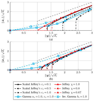
Figure 1: Thresholding function for different priors and parameters for a system with a single block $K=1$, $d_{i}=M=N$ and $\bm{\Phi}=\bm{I}_{N}$. Using a Gamma PDF or inverse Gamma PDF with $b>0$ as hyperprior does not result in a sparse estimate whereas using Jeffrey’s prior or scaled Jeffrey’s prior results in a sparse estimate. Block sizes $d_{i}=2$ (a) and $d_{i}=10$ (b).

Since for this setup $\bm{\Phi}=\bm{I}_{N}$, a perfect estimator for the noiseless case would be $\hat{\bm{x}}_{i}=\bm{y}$ and a sparse estimate can be obtained by thresholding small values of $\|\hat{\bm{x}}_{i}\|$ for $i=1$. Comparing the estimator obtained by different parameters of the generalized inverse Gaussian hyperprior PDF, it can be observed that the Gamma prior and the inverse Gamma prior do not lead to a sparse estimator since $\hat{\bm{x}}_{i}=\bm{0}$ if and only if $\bm{y}=\bm{0}$. This is in line with both the analysis presented in Section V-A and the results from the literature for a non-blocked complex model [19]. When comparing the scaled Jeffrey’s prior and Jeffrey’s prior, we see that both estimators are indeed sparse since many values of $\bm{y}$ lead to $\hat{\bm{x}}_{i}=\bm{0}$. Furthermore, we can see that Jeffrey’s prior without an increased heuristic threshold $\chi$ leads to a “soft” thresholding behavior that smoothly approaches $\hat{\bm{x}}_{i}=\bm{0}$ as $\bm{y}$ gets smaller. Introducing a threshold of $\chi<1$ or utilizing the scaled Jeffrey’s prior is analogous to the ”hard” thresholding approach, where the threshold is determined by either $\chi$ or $c_{i}$. An increase in the threshold results obviously into a sparser estimate. Furthermore, it is noteworthy to highlight the effect of difference different block sizes on the solution ($d_{i}=2$ and $d_{i}=10$ shown in Figure 1a and 1b, respectively). The cutoff value for Jeffery’s prior remains constant even with different thresholds, relative to the average amplitude of the components within the block. However, the likelihood of the average component amplitude being high decreases as the block size increases. This is due to the low likelihood of all amplitudes being high in the same realization. Consequently, a fixed threshold $\chi$ would result in varying false alarm rates depending on the block size. In contrast, using a scaled Jeffrey’s prior leads to a reduction of the cutoff region with an increase in block size, compensating to some extent for the reduction of the false alarm rate.

Finally, from Figure 1 we can see that with $c_{i}$ and $\chi$ tuned to achieve a similar thresholding (e.g. $c_{i}=1$ and $\chi=0.67$ for a block size of $d_{i}=10$), the estimation performance of both estimators is rather similar. Thus, we conclude that the scaled Jeffrey’s prior is to be preferred over Jeffrey’s prior with an additional threshold in order to retain the convergence guarantees of the variational algorithm.

V-D Equivalence to Fast Marginal Likelihood Maximization

In the following, we prove that the proposed fast variational solution to block-SBL using Jeffrey’s prior is equivalent to the fast marginal likelihood maximization scheme of [12]. In [12], the hyperparameters $\bm{\gamma}$ are estimated by maximizing the log marginal likelihood

$$\mathcal{L}_{\text{Ma}}(\bm{\gamma})=2\ln\int p(\bm{y}|\bm{x},\lambda)p(\bm{x}|\bm{\gamma})\,\text{d}\bm{x}$$ (36)

with respect to a single $\gamma_{i}$ at a time in an iterative fashion. We start to prove the equivalence between [12] and our solution by expressing the marginal likelihood (36) as

$$\mathcal{L}_{\text{Ma}}(\bm{\gamma})=\ln|\bm{\Sigma}|+\hat{\lambda}^{2}\bm{y}^{\text{H}}\bm{\Phi}\bm{\Sigma}\bm{\Phi}^{\text{H}}\bm{y}+\sum_{i=1}^{K}d_{i}\ln\gamma_{i}+\text{const.}$$ (37)

after integrating out the weights $\bm{x}$. As derived in Appendix -B, (37) can be expressed as a function of a single prior $\gamma_{i}$ using the Woodbury matrix identity and block matrix determinant lemma as

$$\mathcal{L}_{\text{Ma}}(\bm{\gamma}) =\mathcal{L}_{\sim i}(\bm{\gamma}_{\sim i})+\mathcal{L}_{i}(\gamma_{i})$$

$$=\mathcal{L}_{\sim i}(\bm{\gamma}_{\sim i})+\sum_{l=1}^{d_{i}}\ln\bigg{(}\frac{\gamma_{i}s_{i,l}}{1+\gamma_{i}s_{i,l}}\bigg{)}-\frac{\gamma_{i}|q_{i,l}|^{2}}{(1+\gamma_{i}s_{i,l})^{2}}$$ (38)

where $\bm{\gamma}_{\sim i}$ denotes the vector $\bm{\gamma}$ with the element $\gamma_{i}$ removed and $\mathcal{L}_{\sim i}(\bm{\gamma}_{\sim i})$ is some function which does not depend on $\gamma_{i}$. The marginal likelihood is maximized by finding the maximum of (V-D) as $\frac{\text{d}}{\text{d}\gamma_{i}}\mathcal{L}_{i}(\gamma_{i})=0$. The derivative of (V-D) is

$$\frac{\text{d}}{\text{d}\gamma_{i}}\mathcal{L}_{i}(\gamma_{i})=\sum_{l=1}^{d_{i}}\frac{1}{\gamma_{i}}\frac{1}{1+\gamma_{i}s_{i,l}}-\frac{|q_{i,l}|^{2}}{(1+\gamma_{i}s_{i,l})^{2}}$$ (39)

Thus, the condition $\frac{\text{d}}{\text{d}\gamma_{i}}\mathcal{L}_{i}(\gamma_{i})=0$ can be expressed as

$$0 =\gamma_{i}\sum_{l=1}^{d_{i}}\bigg{(}\big{(}\gamma_{i}s_{i,l}^{2}+|q_{i,l}|^{2}+s_{i,l}\big{)}\prod_{j=1,j\neq l}^{d_{i}}(1+\gamma_{i}s_{i,l})^{2}\bigg{)}$$

$$\qquad-d_{i}\prod_{l=1}^{d_{i}}(1+\gamma_{i}s_{i,l})^{2}$$

$$=\gamma_{i}B_{i}(\gamma_{i})-d_{i}A_{i}(\gamma_{i})\,.$$ (40)

applying the definitions (32) and (33). Comparing (V-D) with the polynomials $G_{i}(\hat{\gamma}_{i})$ in the fifth column of Table I, we recognize that the extrema of the marginalized likelihood with respect to a single $\gamma_{i}$ correspond to the fixed points of the recurrent relation $f_{i}$ in the fast variational solution in case Jeffrey’s prior is used. Hence, showing that the two approaches are equivalent.

VI Numerical Evaluation

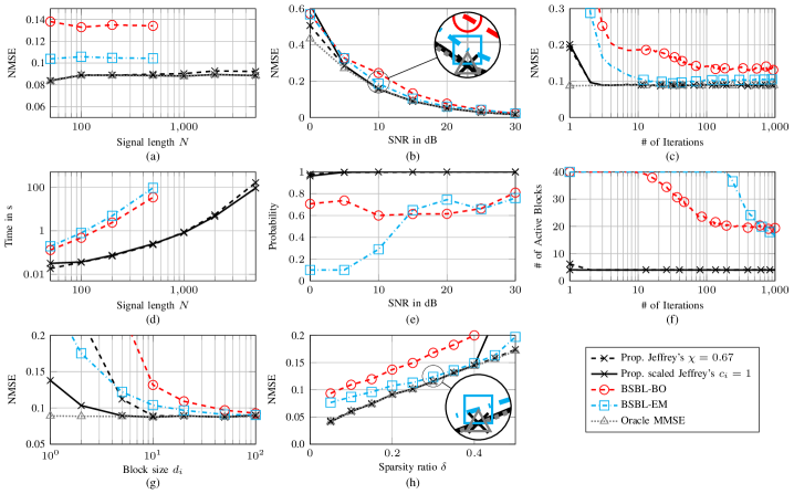
Figure 2: Performance of the proposed algorithm using a dictionary matrix with Gaussian distributed entries averaged over 100 realizations. NMSE as function of the signal length (a), SNR (b) and the number of iterations (c). The runtime of each algorithm as a function of the signal length is shown in (d). Classification probability of correctly classifying each block as zero/nonzero as a function of the SNR (e) and the number of active blocks $(\hat{\bm{x}}_{i}\neq\bm{0}$) as function of the number of iterations (f). Further evaluation of the NMSE over block size (g) and sparsity ratio (h). Unless otherwise stated, the following parameters were used in the simulations. $N=200$, $M=2N$, $\text{SNR}=15\,\text{dB}$, $\delta=0.2$ and $d_{i}=10$ $\forall$ $i$.

To investigate the performance of the algorithm, we generate an dictionary matrix with $M=2N$ columns and assume $N=200$ measurements are obtained unless otherwise stated. The elements of the dictionary matrix are drawn from independent zero-mean normal distributions with unit variance and each column $\bm{\phi}_{k}$ of $\bm{\Phi}$ is normalized such that $\|\bm{\phi}_{k}\|=1$. The the corresponding weight vector $\bm{x}$ is partitioned into blocks with an equal block size of $d_{i}=10$ $\forall$ $i$. We selected a number of blocks at randomly chosen locations such that the desired sparsity ratio $\delta=\frac{\|\bm{x}\|_{0}}{N}=0.2$ was achieved. For these nonzero blocks we draw $\bm{x}_{i}$ from a Gaussian distribution with zero mean and unit variance while for the remaining blocks $\bm{x}_{i}=0$. The location of the nonzero blocks is unknown to the algorithm. The noise precision $\lambda$ is chosen, such that the signal-to-noise ratio (SNR) defined as $\text{SNR}=\frac{\lambda\|\bm{\Phi}\bm{x}\|^{2}}{N}$ equals $15\,\text{dB}$. As performance metric we use the normalized mean squared error (NMSE)defined as $\text{NMSE}=\frac{\|\bm{x}-\hat{\bm{x}}\|^{2}}{\|\bm{x}\|^{2}}$, averaged over 100 simulation runs. We use Jeffrey’s prior for the noise precision $p(\lambda)$, which is obtained by $\epsilon=\eta=0$ in (7). Two variants of the proposed method are evaluated. Once using a Jeffrey’s prior, obtained by $a_{i}=b_{i}=c_{i}=0$ in (15), as hyperprior $p(\gamma_{i})$ and a threshold of $\chi=0.67$, and once using the scaled Jeffrey’s prior with $c_{i}=1$ as hyperprior $p(\gamma_{i})$. Since we are interested in sparse estimators, we did not consider the non-sparse variants of the hyperprior. As comparison methods we use two variants of the EM-based block-SBL algorithm from [9]. The comparison algorithms apply the EM algorithm directly (BSBL-EM) or use a bounded-optimization approach to increase the convergence speed of the EM algorithm (BSBL-BO). Note, that the BSBL-EM algorithm is equivalent to the variational BSBL algorithm [15] using Jeffrey’s prior as hyperprior. For all algorithms we assumed that $\bm{B}_{i}=\bm{I}$ is a known and fixed parameter. We also include an “oracle” minimum mean squared error (MMSE) estimator, which is given the true locations of the nonzero blocks and calculates the weights of the nonzero blocks using the pseudoinverse of the corresponding columns of the dictionary as reference.

Figure 2a-2c depicts the NMSE of the algorithms as a function of the signal length $N$, the SNR and number of iterations. We define the number of iterations as the number of times the main loop of the algorithm is repeated, i.e. the amount of times all variables $\hat{\bm{x}}$, $\hat{\bm{\Sigma}}$, $\hat{\lambda}$ and $\hat{\gamma}_{1}\cdots\hat{\gamma}_{K}$ are updated. Figure 2d shows the runtime of the algorithms again as function of the signal length $N$. For $N=500$, the proposed method is faster by approximately 2 orders of magnitude compared to the two BSBL variants [9] while achieving an NMSE virtually identical to that of the oracle MMSE estimator. As shown in Figures 2b and 2c, an NMSE almost identical to that of the oracle estimator is achieved already after 3 iterations and over a wide range of SNRs. Figure 2e shows the empirical probability of correctly estimating any $\hat{\gamma}_{i}$ as converged or diverged (i.e. the empirical probability of classifying each block correctly as zero or nonzero block). While the proposed method classifies the blocks correctly as zero or nonzero almost all the time, both variants of the BSBL algorithm significantly overestimated the number of nonzero blocks. The difference in the runtime of the algorithms can be explained by Figures 2c and 2f. While our proposed algorithm converges to an NMSE estimate virtually identical that of the oracle estimator after 3 iterations, the BSBL-BO and BSBL-EM algorithm require more iterations to converge. Furthermore, as detailed in Figure 2f, the proposed algorithm estimates the number of active blocks correctly from the first iteration on. Thus, any operations that require the covariance of the weights $\hat{\bm{\Sigma}}$ can be performed with a small matrix since the entries of $\hat{\bm{\Sigma}}$ corresponding to deactivated blocks are exactly zero. It can be seen in Figure 2f, that the BSBL-BO algorithm keeps all 40 blocks active for the first 10 iterations and then slowly starts to deactivate blocks. The BSBL-EM algorithm keeps all 40 blocks active for the first 100 iterations before it starts to deactivate them. Thus, in addition to requiring more iterations until convergence, each iteration also involves operations with a larger matrix $\hat{\bm{\Sigma}}$. Therefore, each iteration of both BSBL variants is computationally more expensive compared to the proposed algorithm.

Additionally, we evaluate how varying the block size $d_{i}$ and the sparsity ratio $\delta$ affects the algorithm performance in terms of NMSE. To evaluate the performance of the algorithm as function of the block size $d_{i}$, we use $N=500$ while we use $N=200$ for the evaluation over the sparsity ratio $\delta$. Figures 2g and 2h show the NMSE obtained by these numerical experiments. Again, the proposed method outperforms both BSBL variants over most simulated sparsity ratios and SNRs. An evaluation of the runtime and zero/nonzero classification probability was evaluated as well. However we found these results to be similar to the ones in Figure 2d and 2e. Thus, they are omitted for the sake of brevity. In case the block size is varied, the proposed method utilizing the scaled Jeffrey’s prior with $c_{i}=1$ is again superior to both BSBL variants as well as to the proposed method if Jeffrey’s prior is used in combination with a threshold of $\chi=0.67$. The difference between the two variants of the proposed method stems form the dependence of the probability of missed detection and false alarm on the block size, which is more severe for Jeffrey’s prior compared to the scaled Jeffrey’s prior as discussed in Section V-C.

VII Application Example: DOA Estimation

VII-A System Model

Consider an unknown number of $L$ narrowband sources with complex signal amplitudes $s_{l}[t]\in\mathbb{C}$, $l=1,\cdots,L$ located at fixed DOAs $\theta_{l}\in\Theta=[-90^{\circ},90^{\circ})$ in the far field of an array consisting of $N$ sensors, such as a microphone or antenna array. Multiple measurements $\bm{y}_{t}\in\mathbb{C}^{N}$ at different times $t=1,2,\cdots,d$ are obtained. Each measurement is modeled as

$$\bm{y}_{t}=\sum_{l=1}^{L}\bm{\psi}(\theta_{l})s_{l}[t]+\bm{v}_{t}$$ (41)

where $\bm{\psi}(\theta_{l})$ is the steering vector of the array and $\bm{v}_{t}$ is additive noise. We assume that the noise $\bm{v}_{t}$ follows a Gaussian PDF $\mathcal{N}(\bm{v}_{t};\bm{0},\lambda^{-1}\bm{I}$) and is independent across different times $t$. For a linear array, the steering vector is

$$\bm{\psi}(\theta_{l})=\frac{1}{\sqrt{N}}\big{[}1\ e^{-j2\pi\frac{p_{2}}{\mu}\sin\theta_{l}}\ \cdots\ e^{-j2\pi\frac{p_{N}}{\mu}\sin\theta_{l}}\big{]}^{\text{T}}$$ (42)

where $\mu$ is the wavelength of the signal and $p_{n}$ is the distance from sensor 1 to sensor $n$.

An alternative model can be obtained by introducing a search grid of $K$ potential source DOAs $\bar{\bm{\theta}}=[\bar{\theta}_{1}\ \bar{\theta}_{2}\ \cdots\bar{\theta}_{K}]^{\text{T}}$ and corresponding amplitude vectors $\bm{x}^{(t)}$. With this grid we construct a dictionary matrix $\bm{\Psi}=[\bm{\psi}(\bar{\theta}_{1})\ \bm{\psi}(\bar{\theta}_{2})\ \cdots\ \bm{\psi}(\bar{\theta}_{K})]$, such that we approximate (41) as

$$\bm{y}_{t}=\bm{\Psi}\bm{x}^{(t)}+\bm{v}_{t}.$$ (43)

Instead of directly estimating $L$ and the DOAs $\theta_{1}$ through $\theta_{L}$ we obtain a sparse estimate of $\bm{x}^{(t)}$ and use the number of nonzero elements of $\bm{x}^{(t)}$ as estimate $\hat{L}$ of $L$. From the columns of $\bm{\Psi}$ corresponding to the active entries in $\bm{x}^{(t)}$, we can extract DOAs estimates $\hat{\theta}_{l}$, $l=1,\cdots,\hat{L}$.

The locations of the sources are assumed stationary. Therefore, the sparsity profile of $\bm{x}^{(t)}$ at different times $t$ stays constant. Let $\bm{Y}=[\bm{y}_{1}\ \bm{y}_{2}\ \cdots\bm{y}_{d}]$, $\bm{X}=[\bm{x}^{(1)}\ \bm{x}^{(2)}\ \cdots\ \bm{x}^{(d)}]$ and $\bm{V}=[\bm{v}_{1}\ \bm{v}_{2}\ \cdots\ \bm{v}_{d}]$, we arrive at the row-sparse MMV signal model

$$\bm{Y}=\bm{\Psi}\bm{X}+\bm{V}.$$ (44)

As discussed in Section II-A, (44) can be rearranged into a block-sparse model. Thus, the row-sparse matrix $\bm{X}$ can be estimated using the presented algorithm.

Note, that in this model the weights in each row of $\bm{X}$, (i.e. each block $\bm{x}_{i}$ of $\bm{x}$) are either zero or correspond to the amplitudes of a source over time $\bm{x}_{i}=\big{[}s_{l}[1]\ s_{l}[2]\ \cdots\ s_{l}[d]\big{]}^{\text{T}}$. Thus, any prior knowledge about these source amplitudes can be incorporated in the matrix $\bm{B}_{i}$.

VII-B DOA Estimation Results

Since the BSBL algorithms from [9] are not applicable for a complex valued signal model, we compare our algorithm against the multi-snapshot SBL-based DOA estimation algorithm in [20] termed DOA-SBL. Since in this case the actual weights $\bm{X}$ are of secondary interest, we resort to the optimal subpattern assignment (OSPA) metric [34] of the estimated DOAs $\hat{\theta}_{l}$, $l\in\{1,\cdots,\hat{L}\}$ to evaluate the performance of the algorithms. The OSPA is a metric which considers both the actual estimation error as well as the error in estimating the model order (i.e. the number of missed detection and false alarms). As parameters for the OSPA, we set the order to $1$ and use a cutoff-distance of $5^{\circ}$. Since the DOA-SBL algorithm does not directly estimating a sparse weight vector, we evaluate two versions of this algorithm. Let $\gamma_{i,\text{DOA-SBL}}$ and $\sigma^{2}_{\text{DOA-SBL}}$ denote the prior variances and noise variance estimated by [20]. We define the component SNR of the $i$-th block as $\text{SNR}_{i,\text{DOA-SBL}}=\frac{\gamma_{i,\text{DOA-SBL}}}{\sigma^{2}_{\text{DOA-SBL}}}$. We consider all DOAs $\hat{\theta}_{i}$ which have an associated component SNR above a certain threshold as first variant of the DOA-SBL algorithm. Based on preliminary simulations, we adapted the threshold to maximize the performance of the DOA-SBL algorithm in our simulated scenarios. As an additional comparison, we also consider an oracle variant of the algorithm which is given the true number of components $L$ and estimates $\hat{\theta}_{l}$ as the DOAs corresponding to the $L$ blocks with largest component SNR. To account for the increasing processing gain at increasing arrays sizes, we define the array SNR as for snapshot $t$ as $\text{SNR}_{\text{A}}=\lambda\|\bm{\Psi}\bm{x}^{(t)}\|^{2}$.

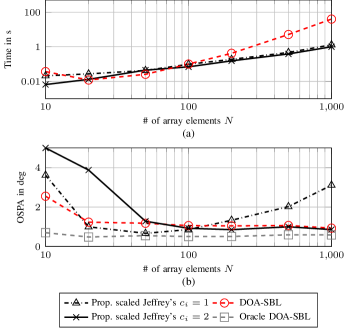
Figure 3: Runtime comparison (a) and OSPA (b) of the proposed method with the DOA-SBL algorithm [20] as function of the number of array elements at an $\text{SNR}_{\text{A}}=10\,\text{dB}$ given a single snapshot $d=1$.

Single-Snapshot Estimation Performance

For the first experiment, we analyse the runtime and estimation accuracy as a function of the number of array elements $N$. We generate a dictionary with $M=2N$ entries spaced such that $\sin(\bar{\theta}_{m})$ forms a regular grid. We simulate 3 sources located at the grid points closest to $\{-2^{\circ},3^{\circ},50^{\circ}\}$ with amplitudes drawn randomly from a zero-mean complex Gaussian distribution with unit variance and consider only a single snapshot $d=1$. For the DOA-SBL algorithm, we calculate the OSPA based on all blocks with component SNR $\geq 10\,\text{dB}$. To illustrate the effect of the parameter $c_{i}$, we use two variants of our algorithm. Both use the scaled Jeffrey’s priors and are parameterized with $c_{i}=1$ and $c_{i}=2$, respectively. Figures 3a and 3b show the runtime and OSPA, respectively, for both algorithms at an $\text{SNR}_{\text{A}}=20\,\text{dB}$. The smallest OSPA is achieved by the oracle DOA-SBL algorithm. This is not surprising, since this algorithm is given the true number of sources in advance. However, knowing the true number of sources is not a realistic assumption for most practical applications. For array sizes of 100 elements and larger, the proposed algorithm parameterized with $c_{i}=2$ is faster than the DOA-SBL algorithm while achieving the same OSPA. For array sizes with less than 100 elements, the OSPA for our algorithm parameterized with $c_{i}=2$ increases rapidly. This is due to some components not being detected in those cases. The parameter $c_{i}$ acts similar to a threshold. Hence, we can increase the detection probability by using a smaller value for $c_{i}$. Consequently, this also leads to an increased false alarm rate. The increased false alarm rate is mostly noticeable at large $N$, due to the larger number of possible DOAs in the grid for large $N$. Hence, by using a smaller $c_{i}$ we can reduce the OSPA at smaller array sizes at the cost of increasing the OSPA at larger array sizes, as shown in Figure 3b. We refer the reader to [32] for a detailed discussion on the relation between the array size and number of false alarms for a similar SBL-based approach.

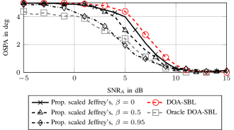
Figure 4: OSPA of the proposed method and the DOA-SBL algorithm [20] as function of the $\text{SNR}_{\text{A}}$ given $d=10$ snapshots with different source correlations $\beta$.

Multi-Snapshot Estimation Performance

Next, we simulate a system with an array consisting of $N=100$ antennas where $d=10$ snapshots are obtained. We simulate three sources at the same DOAs as in the previous experiment. To investigate the effect of intra-block correlations, the source amplitudes $s_{k}[t]$ are generated by a first-order autoregressive model, i.e. $s_{k}[t]=\xi+\beta s_{k}[t-1]$ where $\xi\sim\mathcal{CN}(\xi;0,1)$ is a circularly-symmetric zero-mean complex Gaussian random variable with unit variance. The coefficient $\beta\in\mathbb{C}$ : $|\beta|<1$ can be used to set the correlation between the snapshots over time. The covariance matrix $\bm{\Sigma}_{\text{s}}$ of the samples $s_{k}[t]$ is given as a Toeplitz matrix

$$\bm{\Sigma}_{\text{s}}=\left[\begin{matrix}1&\beta&\cdots&\beta^{d-1}\\ \beta&1&\cdots&\beta^{d-2}\\ \vdots&\vdots&\ddots&\vdots\\ \beta^{d-1}&\beta^{d-2}&\cdots&1\end{matrix}\right].$$ (45)

We evaluate three different cases. (i) no correlation $\beta=0$, (ii) medium correlation $\beta=0.5$ and (iii) strong correlation $\beta=0.95$. For the proposed algorithm we set $\bm{B}_{i}=\bm{\Sigma}_{\text{s}}^{-1}$ $\forall$ $i$ to exploit this information. The correlation between the source amplitudes provides additional statistical information which can be used to separate true sources from the additive white noise. Therefore, the probability of false alarms gets smaller with increasing correlation $\beta$. To achieve an (approximately) constant false alarm rate for our algorithm, we parameterize the scaled Jeffrey’s prior with $c_{i}=2$ for the case of no correlation (i) and medium correlation (ii), and use $c_{i}=1.5$ for high correlation (iii), based on preliminary simulations. For the DOA-SBL algorithm, we calculate the OSPA based on all blocks with a component SNR $\geq 2\,\text{dB}$, based on the same preliminary simulations. The performance of the DOA-SBL algorithm is approximately the same in all three cases, since it can not exploit the additional information resulting from the correlation of the source amplitudes. Thus, we plot the performance of the DOA-SBL only for case (i). Figure 4 depicts the OSPA of both algorithms as a function of the $\text{SNR}_{\text{A}}$. For $\text{SNR}_{\text{A}}<0\,\text{dB}$ and $\text{SNR}_{\text{A}}>10\,\text{dB}$, the estimation either fails due to the high noise level or is trivial. Thus the performance of both algorithms is approximately the same in these regions. In the transition region $0\,\text{dB}\leq\text{SNR}_{\text{A}}\leq 10\,\text{dB}$, the proposed algorithm achieves a smaller OSPA than the DOA-SBL algorithm for all three cases. With increasing correlation, the performance of the proposed algorithm improves. For the case of high correlation (iii), the performance of the proposed algorithm is practically the same as the performance of the oracle DOA-SBL algorithm which is given the true number of sources $L$. We refer the reader to [8] for a more in-depth investigation and discussion of the effects of the intra-block correlation $\bm{B}_{i}$ as well as for suggestions on how to estimate this matrix efficiently without introducing too many additional parameters.

Note, that in any practical example the DOAs will not align exactly with the search grid of potential DOAs. This mismatch introduces errors and complicates the estimation process. This can be counteracted e.g. by using a variational-EM approach similar to [14, 21] to optimizing the ELBO over the estimated source locations $\hat{\theta}_{l}$ in addition to the variational parameters. Furthermore, [30] directly integrates the estimation of the parameters $\hat{\theta}_{l}$ into the variational framework in order to obtain (approximate) posterior distributions $q(\theta_{l})$. However, we consider these off-grid approaches outside the scope of this work.

VIII Conclusion

We derived a fast update rule for the variational Bayesian approach to block-SBL. Iterating the update equation for the approximating PDF of the weights and hyperparameters is expressed as a first-order recurrence from the previous parameter set to the next. We showed how the fixed points of the recurrent relation can be obtained as the roots of a polynomial. Furthermore, by proving that the recurrent relation is a strictly increasing rational function, we are able to determine if the sequence converges and, if it does converge, we can determine its limit. Hence, we can check for convergence/divergence and update each hyperparameter to its asymptotic value in a single step.

Using numerical simulations, we show that the proposed fast update rule improves the run time of the variational block-sparse SBL algorithm [9] by two orders of magnitude. Moreover, the proposed algorithm is shown to achieve a smaller NMSE over a wide range of signal lengths, SNRs, block sizes and sparsity ratios than the comparison algorithms. Additionally, the proposed algorithm is also applied to DOA estimation. Our results demonstrate that (i) our algorithm is able to outperform similar SBL-based DOA estimation algorithms in terms of computation time while achieving a similar performance for single-snapshot DOA estimation and (ii) achieves a smaller OSPA than the comparison DOA estimation algorithm in a low-SNR multiple-snapshot DOA estimation scenario where the source amplitudes are correlated over the snapshots.

A promising direction for future research is the extension of the presented method to include the estimation of the size of each block, or, to a parametrized continuous (infinite) dictionary matrix similar to our recent work [21]. Another interesting direction for future research is the combination of the presented method with belief propagation algorithms for joint channel estimation and decoding [25] or sequential tracking of time variant channels [36] in multi-input multiple-output communication systems, which are often modeled to be block-sparse [24, 23].

-A Proof that $h_{i}$ is Strictly Decreasing

To obtain a more convenient expression for $h_{i}(\hat{\gamma}_{i})=B_{i}(\hat{\gamma}_{i})/A_{i}(\hat{\gamma}_{i})$, we express the polynomial $B_{i}(\hat{\gamma}_{i})$ given in (33) as the product of $A_{i}(\hat{\gamma}_{i})$ defined in (32) and some expression

$$B_{i}(\hat{\gamma}_{i}) =\sum_{l=1}^{d_{i}}(\hat{\gamma}_{i}s_{i,l}^{2}+|q_{i,l}|^{2}+s_{i,l})\prod_{j=1,j\neq i}^{d_{i}}(1+\hat{\gamma}_{i}s_{i,j})^{2}$$

$$=\sum_{l=1}^{d_{i}}\frac{\hat{\gamma}_{i}s_{i,l}^{2}+|q_{i,l}|^{2}+s_{i,l}}{(1+\hat{\gamma}_{i}s_{i,l})^{2}}\prod_{j=1}^{d_{i}}(1+\hat{\gamma}_{i}s_{i,j})^{2}$$

$$=A_{i}(\hat{\gamma}_{i})\cdot\sum_{l=1}^{d_{i}}\frac{\hat{\gamma}_{i}s_{i,l}^{2}+|q_{i,l}|^{2}+s_{i,l}}{(1+\hat{\gamma}_{i}s_{i,l})^{2}}\,.$$ (46)

Inserting (46) into (23), we rewrite $h_{i}(\hat{\gamma}_{i})$ as

$$h_{i}(\hat{\gamma}_{i})=\frac{B_{i}(\hat{\gamma}_{i})}{A_{i}(\hat{\gamma}_{i})}=\sum_{l=1}^{d_{i}}\frac{\hat{\gamma}_{i}s_{i,l}^{2}+|q_{i,l}|^{2}+s_{i,l}}{(1+\hat{\gamma}_{i}s_{i,l})^{2}}$$ (47)

Taking the derivative of $h_{i}(\hat{\gamma}_{i})$ with respect to $\hat{\gamma}_{i}$ results in

$$\frac{\text{d}}{\text{d}\hat{\gamma}_{i}}h_{i}(\hat{\gamma}_{i}) =\sum_{l=1}^{d_{i}}\frac{\text{d}}{\text{d}\hat{\gamma}_{i}}\frac{\hat{\gamma}_{i}s_{i,l}^{2}+|q_{i,l}|^{2}+s_{i,l}}{(1+\hat{\gamma}_{i}s_{i,l})^{2}}$$

$$=-\sum_{l=1}^{d_{i}}\frac{\hat{\gamma}_{i}s_{i,l}^{3}+2s_{i,l}|q_{i,l}|^{2}+s_{i,l}^{2}}{(1+\hat{\gamma}_{i}s_{i,l})^{3}}\,.$$ (48)

Since $s_{i,l}>0$ and $|q_{i,l}|^{2}>0$, we have $\frac{\text{d}h_{i}(\hat{\gamma}_{i})}{\text{d}\hat{\gamma}_{i}}<0$ $\forall$ $\hat{\gamma}_{i}\in\mathbb{R}_{\geq 0}$. Thus, proving that $h_{i}$ is a strictly decreasing function on the domain $\mathbb{R}_{\geq 0}$.

-B Detailed Derivations for the Proof of Equivalence

Let $\bm{\Phi}_{i}$ denote all columns of the dictionary matrix which correspond to the $i$-th block and $\bm{\Phi}_{\sim i}$ all remaining columns of $\bm{\Phi}$, such that $\bm{\Phi}=[\bm{\Phi}_{\sim i}\hskip 2.84526pt\bm{\Phi}_{i}]$. Similarly, let $\bm{B}_{\sim i}$ be a diagonal matrix with the blocks $\gamma_{k}\bm{B}_{k}$ $\forall$ $k\in\{1,\,2,\,\cdots,\,K\}\backslash\{i\}$ on its main diagonal, such that we can express $\bm{\Sigma}^{-1}$ as a block matrix

$$\bm{\Sigma}^{-1}=\left[\begin{matrix}\lambda\bm{\Phi}_{\sim i}^{\text{H}}\bm{\Phi}_{\sim i}+\bm{B}_{\sim i}&\lambda\bm{\Phi}_{\sim i}^{\text{H}}\bm{\Phi}_{i}\\ \lambda\bm{\Phi}_{i}^{\text{H}}\bm{\Phi}_{\sim i}&\lambda\bm{\Phi}_{i}^{\text{H}}\bm{\Phi}_{i}+\gamma_{i}\bm{I}\end{matrix}\right]\,.$$ (49)

Denoting $\bm{\Sigma}_{\sim i}=(\lambda\bm{\Phi}_{\sim i}^{\text{H}}\bm{\Phi}_{\sim i}+\bm{B}_{\sim i})^{-1}$ and $\bm{\Sigma}_{i}=(\lambda\bm{\Phi}_{i}^{\text{H}}\bm{\Phi}_{i}-\lambda^{2}\bm{\Phi}_{i}^{\text{H}}\bm{\Phi}_{\sim i}\bm{\Sigma}_{\sim i}\bm{\Phi}_{\sim i}^{\text{H}}\bm{\Phi}_{i})^{-1}$, we use the block matrix determinant lemma to express

$$\ln|\bm{\Sigma}| =-\ln|\bm{\Sigma}^{-1}|=\ln|\bm{\Sigma}_{\sim i}|-\ln|\bm{\Sigma}_{i}^{-1}+\gamma_{i}\bm{I}|$$

$$=\ln|\bm{\Sigma}_{\sim i}|-\sum_{l=1}^{d_{i}}\ln\big{(}\gamma_{i}+\frac{1}{s_{i,l}}\big{)}\,.$$ (50)

Using the Woodbury matrix identity, we can also make the dependence on $\gamma_{i}$ explicit in the second term in (37)

$$\lambda^{2}\bm{y}^{\text{H}}\bm{\Phi}\bm{\Sigma}\bm{\Phi}^{\text{H}}\bm{y} =\lambda^{2}\bm{y}^{\text{H}}\bm{\Phi}\big{(}\bar{\bm{\Sigma}}-\bar{\bm{\Sigma}}\bm{E}_{i}(\gamma_{i}^{-1}\bm{I}+\bm{\Sigma}_{i})^{-1}\bm{E}_{i}^{\text{T}}\bar{\bm{\Sigma}})\bm{\Phi}^{\text{H}}\bm{y}$$ (51)

Using the identity (27), expression (51) can be be further simplified to

$$\lambda^{2}\bm{y}^{\text{H}}\bm{\Phi}\bm{\Sigma}\bm{\Phi}^{\text{H}}\bm{y} =\text{const.}-\bm{q}_{i}^{\text{H}}(\gamma_{i}^{-1}\bm{I}+\bm{S}_{i})^{-1}\bm{q}_{i}$$

$$=\text{const.}-\sum_{l=1}^{d_{i}}\frac{\gamma_{i}|q_{i,l}|^{2}}{1+\gamma_{i}s_{i,l}}.$$ (52)

Inserting (-B) and (-B) into (37) we arrive at (V-D).

Given the derivatives $\frac{\text{d}}{\text{d}\gamma_{i}}\ln\frac{\gamma_{i}s_{i,l}}{1+\gamma_{i}s_{i,l}}=\frac{1}{\gamma_{i}}\frac{1}{1+\gamma_{i}s_{i,l}}$ and $\frac{\text{d}}{\text{d}\gamma_{i}}\frac{\gamma_{i}|q_{i,l}|^{2}}{1+\gamma_{i}s_{i,l}}=\frac{|q_{i,l}|^{2}}{(1+\gamma_{i}s_{i,l})^{2}}$, (39) is readily obtained. To arrive at (V-D), we start with $\frac{\text{d}}{\text{d}\gamma_{i}}\mathcal{L}_{i}(\gamma_{i})=0$ and multiply both sides of the equation with $\gamma_{i}\prod_{l=1}^{d_{i}}(1+\gamma_{i}s_{i,l})^{2}$ to obtain

$$0=\sum_{l=1}^{d_{i}}\big{(}1+\gamma_{i}s_{i,l}-\gamma_{i}|q_{i,l}|^{2}\big{)}\prod_{j=1,j\neq l}^{d_{i}}(1+\gamma_{i}s_{i,l})^{2}\,.$$ (53)

Finally, we add $0=\gamma_{i}s_{i,l}+\gamma_{i}^{2}s_{i,l}^{2}-\gamma_{i}s_{i,l}-\gamma_{i}^{2}s_{i,l}^{2}$ into each term in the sum in (53) to arrive at (V-D) after a few algebraic manipulations.

References

• [1] M. F. Duarte and Y. C. Eldar, “Structured compressed sensing: From theory to applications,” IEEE Trans. Signal Process., vol. 59, no. 9, pp. 4053–4085, Sep. 2011.
• [2] O. Barndorff-Nielsen, J. Kent, and M. Sørensen, “Normal variance-mean mixtures and z distributions,” Int. Statist Rev. / Revue Internationale de Statistique, vol. 50, no. 2, pp. 145–159, Aug. 1982.
• [3] M. E. Tipping, “Sparse Bayesian learning and the relevance vector machine,” J. Mach. Learn. Res., vol. 1, pp. 211–244, Jun. 2001.
• [4] A. Faul and M. Tipping, “Analysis of sparse Bayesian learning,” in Advances Neural Inf. Process. Syst., vol. 14, Vancouver, Canada, Dec. 3–8, 2001, pp. 383–389.
• [5] M. E. Tipping and A. C. Faul, “Fast marginal likelihood maximisation for sparse Bayesian models,” in Proc. 9th Int. Workshop Artif. Intell. and Statist., vol. R4, Key West, FL, USA, Jan. 03–06, 2003, pp. 276–283.
• [6] D. P. Wipf and B. D. Rao, “Sparse Bayesian learning for basis selection,” IEEE Trans. Signal Process., vol. 52, no. 8, pp. 2153–2164, Aug. 2004.
• [7] ——, “An empirical Bayesian strategy for solving the simultaneous sparse approximation problem,” IEEE Trans. Signal Process., vol. 55, no. 7, pp. 3704–3716, Jun. 2007.
• [8] Z. Zhang and B. D. Rao, “Sparse signal recovery with temporally correlated source vectors using sparse Bayesian learning,” IEEE J. Sel. Topics Signal Process., vol. 5, no. 5, pp. 912–926, 2011.
• [9] ——, “Extension of SBL algorithms for the recovery of block sparse signals with intra-block correlation,” IEEE Trans. Signal Process., vol. 61, no. 8, pp. 2009–2015, Apr. 2013.
• [10] J. Fang, Y. Shen, H. Li, and P. Wang, “Pattern-coupled sparse Bayesian learning for recovery of block-sparse signals,” IEEE Trans. Signal Process., vol. 63, no. 2, pp. 360–372, Jan. 2015.
• [11] M. Luessi, S. D. Babacan, R. Molina, and A. K. Katsaggelos, “Bayesian simultaneous sparse approximation with smooth signals,” IEEE Trans. Signal Process., vol. 61, no. 22, pp. 5716–5729, Nov. 2013.
• [12] Z. Ma, W. Dai, Y. Liu, and X. Wang, “Group sparse Bayesian learning via exact and fast marginal likelihood maximization,” IEEE Trans. Signal Process., vol. 65, no. 10, pp. 2741–2753, May 2017.
• [13] D. Shutin, T. Buchgraber, S. R. Kulkarni, and H. V. Poor, “Fast variational sparse Bayesian learning with automatic relevance determination for superimposed signals,” IEEE Trans. Signal Process., vol. 59, no. 12, pp. 6257–6261, Dec. 2011.
• [14] D. Shutin, W. Wand, and T. Jost, “Incremental sparse Bayesian learning for parameter estimation of superimposed signals,” in 10th Int. Conf. Sampling Theory and Appl., Bremen, Germany, Jul. 1–5, 2013, pp. 513–516.
• [15] S. D. Babacan, S. Nakajima, and M. N. Do, “Bayesian group-sparse modeling and variational inference,” IEEE Trans. Signal Process., vol. 62, no. 11, pp. 2906–2921, Jun. 2014.
• [16] S. Sharma, S. Chaudhury, and Jayadeva, “Variational Bayes block sparse modeling with correlated entries,” in 24th Int. Conf. Pattern Recognit., Beijing, China, Aug.20–24, 2018, pp. 1313–1318.
• [17] D. G. Tzikas, A. C. Likas, and N. P. Galatsanos, “The variational approximation for Bayesian inference,” IEEE Signal Process. Mag., vol. 25, no. 6, pp. 131–146, Nov. 2008.
• [18] C. M. Bishop, Pattern Recognition and Machine Learning.   Secaucus, NJ, USA: Springer-Verlag New York, Inc., 2006.
• [19] N. L. Pedersen, C. Navarro Manchón, M.-A. Badiu, D. Shutin, and B. H. Fleury, “Sparse estimation using Bayesian hierarchical prior modeling for real and complex linear models,” Signal Process., vol. 115, pp. 94–109, Oct. 2015.
• [20] P. Gerstoft, C. F. Mecklenbräuker, A. Xenaki, and S. Nannuru, “Multisnapshot sparse Bayesian learning for DOA,” IEEE Signal Process. Lett., vol. 23, no. 10, pp. 1469–1473, Oct. 2016.
• [21] J. Möderl, F. Pernkopf, K. Witrisal, and E. Leitinger, “Variational inference of structured line spectra exploiting group-sparsity,” ArXiv e-prints, Mar. 2023. [Online]. Available: https://arxiv.org/abs/2303.03017
• [22] E. Riegler, G. E. Kirkelund, C. N. Manchon, M. A. Badiu, and B. H. Fleury, “Merging belief propagation and the mean field approximation: A free energy approach,” IEEE Trans. Inf. Theory, vol. 59, no. 1, pp. 588–602, Jan. 2013.
• [23] O.-E. Barbu, C. Navarro Manchón, C. Rom, T. Balercia, and B. H. Fleury, “OFDM receiver for fast time-varying channels using block-sparse Bayesian learning,” IEEE Trans. Veh. Technol., vol. 65, no. 12, pp. 10 053–10 057, Dec. 2016.
• [24] R. Prasad, C. R. Murthy, and B. D. Rao, “Joint channel estimation and data detection in MIMO-OFDM systems: A sparse Bayesian learning approach,” IEEE Trans. Signal Process., vol. 63, no. 20, pp. 5369–5382, Oct. 2015.
• [25] G. E. Kirkelund, C. N. Manchon, L. P. B. Christensen, E. Riegler, and B. H. Fleury, “Variational message-passing for joint channel estimation and decoding in MIMO-OFDM,” in 2010 IEEE Global Telecommun. Conf., London, U.K., Dec. 6–10, 2010, pp. 1–6.
• [26] B. Jorgensen, Statistical properties of the generalized inverse Gaussian distribution, ser. Lecture notes in statistics.   New York, NY, USA: Springer-Verlag, 1982, vol. 9.
• [27] W. Rudin, Principles of mathematical analysis, 3rd ed.   New York, NY, USA: McGraw-Hill, 1976.
• [28] A. Edelman and H. Murakami, “Polynomial roots from companion matrix eigenvalues,” Math. Comput., vol. 64, no. 210, pp. 763–776, 1995.
• [29] K. B. Petersen and M. S. Pedersen, The Matrix Cookbook.   Technical University of Denmark, 2012, version Nov. 15, 2012, Accessed: Oct. 2023. [Online]. Available: https://www.math.uwaterloo.ca/~hwolkowi/matrixcookbook.pdf
• [30] M.-A. Badiu, T. L. Hansen, and B. H. Fleury, “Variational Bayesian inference of line spectra,” IEEE Trans. Signal Process., vol. 65, no. 9, pp. 2247–2261, May 2017.
• [31] T. L. Hansen, B. H. Fleury, and B. D. Rao, “Superfast line spectral estimation,” IEEE Trans. Signal Process., vol. 66, no. 10, pp. 2511–2526, Feb. 2018.
• [32] E. Leitinger, S. Grebien, B. Fleury, and K. Witrisal, “Detection and estimation of a spectral line in MIMO systems,” in 2020 54th Asilomar Conf. Signals, Syst. and Computers, Pacific Grove, CA, USA, Nov. 01–04, 2020, pp. 1090–1095.
• [33] S. Grebien, E. Leitinger, K. Witrisal, and B. H. Fleury, “Super-resolution estimation of UWB channels including the diffuse component – an SBL-inspired approach,” ArXiv e-prints, Aug. 2023. [Online]. Available: https://arxiv.org/abs/2308.01702
• [34] D. Schuhmacher, B.-T. Vo, and B.-N. Vo, “A consistent metric for performance evaluation of multi-object filters,” IEEE Trans. Signal Process., vol. 56, no. 8, pp. 3447–3457, Aug. 2008.
• [35] Y. Park, F. Meyer, and P. Gerstoft, “Graph-based sequential beamforming,” J. Acoustical Soc. Amer., vol. 153, no. 1, pp. 723–737, Jan. 2023.
• [36] X. Li, E. Leitinger, A. Venus, and F. Tufvesson, “Sequential detection and estimation of multipath channel parameters using belief propagation,” IEEE Trans. Wireless Commun., vol. 21, no. 10, pp. 8385–8402, Oct. 2022.