Inspecting molecular aggregate quadratic vibronic coupling effects using squeezed coherent states

Abstract

We present systematic comparison of three quantum mechanical approaches describing excitation dynamics in molecular complexes using the Time-Dependent variational principle (TDVP) with three increasing sophistication trial wavefunctions (ansatze): Davydov $\text{D}_{2}$, squeezed $\text{D}_{2}$ ($\text{sqD}_{2}$) and a numerically exact multiple $\text{D}_{2}$ ($\text{mD}_{2}$) ansatz in order to characterize validity of the $\text{sqD}_{2}$ ansatze. Numerical simulation of molecular aggregate absorption and fluorescence spectra with intra- and intermolecular vibrational modes, including quadratic electron-vibrational (vibronic) coupling term, which is due to vibrational frequency shift upon pigment excitation is presented. Simulated absorption and fluorescence spectra of J type molecular dimer with high frequency intramolecular vibrational modes obtained with $\text{D}_{2}$ and $\text{sqD}_{2}$ ansatze matches spectra of $\text{mD}_{2}$ ansatz only in the single pigment model without quadratic vibronic coupling. In general, the use of $\text{mD}_{2}$ ansatz is required to model accurate dimer and larger aggregate’s spectra. For a J dimer aggregate coupled to a low frequency intermolecular phonon bath, absorption and fluorescence spectra are qualitatively similar using all three ansatze. The quadratic vibronic coupling term in both absorption and fluorescence spectra manifests itself as a lineshape peak amplitude redistribution, static frequency shift and an additional shift, which is temperature dependent. Overall the squeezed $\text{D}_{2}$ model does not result in considerable improvement of simulation results compared to the simplest Davydov $\text{D}_{2}$ approach.

I Introduction

A fundamental aspect of the physics of optically excited molecules and their complexes is the transport of excitation energy. Electronic and vibronic couplings are two aspects that are crucial to this process [1]. Complex quantum dynamics of electronic and vibrational excitations are produced as a result of intermolecular interactions right after the optical excitation. Their interplay is essential for effective photosynthetic machinery in a natural setting where the energy transfer, relaxation, and charge transfer play a crucial role in initial stages of solar energy conversion [2, 3].

The wavefunction-based TDVP method can be used to simulate molecular aggregate excitation dynamics as well as their optical spectra with respect to an ansatz (or parameterization form), which should be sufficiently sophisticated to describe the aggregate’s essential vibronic features. One family of wavefunctions is called Davydov’s ansatze [4, 5, 6], which utilize Gaussian wavepackets, also known as coherent states (CS), to represent vibronic states of molecular aggregate. It has been extensively used to compute spectra of molecules as well as to examine excitation relaxation dynamics in single molecules and their molecular aggregates [7, 8, 9, 10, 11, 12, 13, 14].

The trial wavefunction’s selection greatly influences how accurate the method is. It has been shown, that in some cases, for precise modeling of molecular aggregates, the $D_{2}$ ansatz falls short [15], however, accuracy of vibrational mode representation can be improved by expanding the available parameter space. The most potent approach is to consider a superposition of multiple $\text{D}_{2}$ ansatze, known as the multi-Davydov $\text{D}_{2}$ ansatz. It considerably increases accuracy, making TDVP with $\text{mD}_{2}$ a numerically exact method. Spin-boson models [16], nonadiabatic dynamics of molecules’ dynamics [17, 10], linear and nonlinear spectra of molecular aggregates [11, 15, 18] have all been investigated using TDVP with $\text{mD}_{2}$.

Instead of considering superposition of ansatze, which is equivalent to complete quantum treatment, one can expand available state space of the $\text{D}_{2}$ ansatz incrementally. One approach is to replace the CS with squeezed coherent states (sqCS), which has additional degrees of freeedom (DOFs) which allow for wavepacket to contract and expand along coordinate and momentum axes in it’s phase space. Presumably this should allow sqCS to better represent complicated structure of realistic vibrational mode wavepackets, which become non-Gaussian due to both electronic [18] and quadratic vibronic [13, 19, 10] couplings.

In this work, we aim to compare accuracy of TDVP with three increasing sophistication ansatze: the regular Davydov $\text{D}_{2}$, $\text{sqD}_{2}$ with sqCS and an exact $\text{mD}_{2}$ ansatz by analysing simulated absorption and fluorescence spectra of a J-type dimer couped to high frequency (intra-) and low freqency intermolecular vibrational modes. In addition, we also consider the quadratic vibronic coupling term, which induce wavepacket non-Gaussianity.

The rest of the paper is organized as follows: in Subsection II.A we describe quadratic vibronic molecular aggregate model, considered ansatze and shortly mention an approach to include finite temperature into the model. In Subsection II.B we present theory of absorption and fluorescence spectra using TDVP approach. In Section III we analyze and compare J aggregate absorption and fluorescence spectra in three vibrational mode regimes. Results are discussed and conclusions are given in Section IV.

II Theory

II.1 Electron-vibrational molecular aggregate model theory

The generic model system is a molecular aggregate made of $N$ chromophores with resonant interaction between them. Each chromophore corresponds to a single pigment molecule (site) which is a two-level electronic quantum system with ground and excited states. Moreover, each pigment is coupled to a set of vibrational degrees of freedom (DOF) corresponding to either intra- or intermolecular vibrational modes. Vibrations are explicitly modeled by quantum harmonic oscillators (QHO). The total system Hamiltonian can then be written as [1, 20, 3, 21]

$$\hat{H}=\hat{H}_{\text{S}}+\hat{H}_{\text{V}}+\hat{H}_{\text{S-V}}+\hat{H}_{\text{S-V}^{2}},$$ (1)

where $\hat{H}_{\text{S}}$ represents site Hamiltonian, $\hat{H}_{\text{V}}$ is a vibrational Hamiltonian, $\hat{H}_{\text{S-V}}$ is a first-order interaction term between sites and vibrational modes, and $\hat{H}_{\text{S-V}^{2}}$ is the quadratic site-vibration coupling term. All of the above are explicitly expressed as

$$\hat{H}_{\text{S}}= \sum_{n}\varepsilon_{n}\hat{a}_{n}^{\dagger}\hat{a}_{n}+\sum_{n,m}^{n\neq m}V_{nm}\hat{a}_{n}^{\dagger}\hat{a}_{m},$$ (2)

$$\hat{H}_{\text{V}}= \sum_{k,q}\omega_{kq}^{g}\hat{b}_{kq}^{\dagger}\hat{b}_{kq},$$ (3)

$$\hat{H}_{\text{S-V}}= -\sum_{n}\hat{a}_{n}^{\dagger}\hat{a}_{n}\sum_{q}\omega_{nq}^{e}f_{nq}\left(\hat{b}_{nq}^{\dagger}+\hat{b}_{nq}\right),$$ (4)

$$\hat{H}_{\text{$\text{S-V}^{2}$}}= \frac{1}{4}\sum_{n}\hat{a}_{n}^{\dagger}\hat{a}_{n}\sum_{q}\left(w_{nq}^{e}-w_{nq}^{g}\right)\left(\hat{b}_{nq}^{\dagger}+\hat{b}_{nq}\right)^{2},$$ (5)

where $\varepsilon_{n}$ denotes the $n$th site electronic excitation energy, whichincludes molecular reorganization energy, equal to $\Lambda_{n}=\sum_{q}\omega_{nq}^{e}f_{nq}^{2}$. where summation index $q$ runs over vibrational modes. $V_{nm}$ is the resonant coupling between the $n$th and $m$th site, $\hat{a}_{n}^{\dagger}$ $\left(\hat{a}_{n}\right)$ are the creation (annihilation) operators of chromophore electronic excitation, $\hat{b}_{nq}^{\dagger}$ $\left(\hat{b}_{nq}\right)$ are creation (annihilation) operators of vibrational excitations. The linear vibronic coupling strength is given by dimensionless amplitude $f_{nq}$. The quadratic vibronic coupling term, $\hat{H}_{\text{$\text{S-V}^{2}$}}$, becomes relevant once the vibrational mode frequencies in electronic ground state, $\omega_{nq}^{g}$, are different from the ones in excited state, $\omega_{nq}^{e}$, otherwise this term does not contribute [13, 22, 23, 24, 25, 26, 10].

To obtain linear absorption and fluorescence spectrum of the presented vibronic model, we will be using the TDVP method, which will be applied to three parameterized wavefunction ansatze with increasing sophistication. All of them are based on the Davydov $\text{D}_{2}$ ansatz. First of, the least sophisticated ansatz we will be testing, is the Davydov $\text{D}_{2}$ ansatz. It considers a superposition of singly excited aggregate configurations $|n\rangle=|1\rangle_{n}\prod_{m\neq n}|0\rangle$ [27, 1], with time-dependent amplitudes $\alpha_{n}\left(t\right)$, while vibrational QHO states are expanded in terms of CS. These are obtained by applying the translation operator

$$\hat{D}\left(\lambda_{kq}\left(t\right)\right)=\exp\left(\lambda_{kq}\left(t\right)\hat{b}_{kq}^{\dagger}-\text{h.c.}\right),$$ (6)

with complex time-dependent displacement parameters, $\lambda_{kq}$, to the QHO vacuum state denoted by $|0\rangle_{kq}$. Then the $\text{D}_{2}$ ansatz is defined as

$$|\Psi_{\text{D}_{2}}\left(t\right)\rangle=\sum_{n}\alpha_{n}\left(t\right)|n\rangle\prod_{k,q}|\lambda_{kq}\left(t\right)\rangle.$$ (7)

In order to increase the complexity of ansatz to better represent a complicated vibronic model states, in addition to the translation operator, we can additionally apply the squeeze operator

$$\hat{S}\left(\zeta_{kq}\left(t\right)\right)=\exp\left(\frac{1}{2}\left(\zeta_{kq}^{*}\left(t\right)\hat{b}_{kq}^{2}-\text{h.c.}\right)\right),$$ (8)

with complex-valued squeeze parameter $\zeta_{kq}(t)$, which squeezes the Gaussian wavepacket and only then shifts the resulting squeezed state along the coordinate and momentum axes. The resulting state

$$\hat{D}\left(\lambda_{kq}\left(t\right)\right)\hat{S}\left(\zeta_{kq}\left(t\right)\right)|0\rangle_{kq}=|\lambda_{kq}\left(t\right),\zeta_{kq}\left(t\right)\rangle,$$ (9)

is called a sqCS. For convenience, we express complex squeeze parameter $\zeta_{kq}(t)$ in its polar form $\zeta_{kq}(t)=r_{kq}(t)e^{\text{i}\theta_{kq}(t)}$ where squeeze amplitude $r_{kq}(t)$ and squeeze angle $\theta_{kq}(t)$ are now real time-dependent parameters. Then the squeezed $\text{sqD}_{2}$ ansatz is defined as

$$|\Psi_{\text{sqD}_{2}}\left(t\right)\rangle=\sum_{n}\alpha_{n}\left(t\right)|n\rangle\prod_{k,q}|\lambda_{kq}\left(t\right),\zeta_{kq}\left(t\right)\rangle.$$ (10)

Even more general approach to constructing the ansatz is to consider a superposition of multiple copies of the $\text{D}_{2}$ ansatz. It has been termed by the multiple Davydov $\text{D}_{2}$, $\text{mD}_{2}$ ansatz, and is defined as

$$|\Psi_{\text{mD}_{2}}\left(t\right)\rangle=\sum_{i=1}^{M}\left(\sum_{n}\alpha_{i,n}\left(t\right)|n\rangle\prod_{k,q}|\lambda_{i,kq}\left(t\right)\rangle\right),$$ (11)

where each $i-$th multiple corresponds to a superposition of electronic state excitations accompanied by the vibrational state of an aggregate. By increasing the number of multiples considered, $M$, ansatz state space is expanded accordingly. Note, that $\text{mD}_{2}$ ansatz with $M=1$ simplifies to the $\text{D}_{2}$ ansatz, while an arbitrary wavefunction can be expressed when $M\to\infty$, making the approach exact.

Time evolution of considered ansatze are obtained by solving their respective equations of motion (EOM), which are given Appendix A. A more in depth discussion of $\text{mD}_{2}$ ansatz EOM numerical implementation can be found in Refs. [18, 28].

Inclusion of additional statistical physics concepts are required in order to simulate finite temperature of the model. The thermal ensemble will be constructed by considering independent wavefunction trajectories $\gamma$, each with different initial conditions, and thus energies. Notice that time propagation of wavefunction fully conserves the total energy of each trajectory.

Considering excitation process, prior to molecular aggregate excitation via an external field, the aggregate is in its electronic ground state $|0\rangle$, while vibrational DOFs are thermally excited. Thus QHO modes follow statistics of the canonical ensemble with respect to aggregate ground electronic state. Characterization of the vibrational manifold is straightfoward because all oscillators in electronic ground state state are uncoupled. Diagonal density operator of a single QHO can be written in the basis of CS with quasiprobability distribution function [29, 8, 30, 31]

$$\mathcal{P}^{\left(\text{g/e}\right)}\left(\lambda\right)=\mathcal{Z}^{-1}\exp\left(-\left|\lambda\right|^{2}\left(\text{e}^{\frac{\omega_{g/e}}{k_{\text{B}}T}}-1\right)\right),$$ (12)

where $\mathcal{Z}$ is the partition function of QHO, $k_{\text{B}}$ is the Boltzmann constant and $T$ is the temperature. By sampling $\mathcal{P}^{\left(\text{g}\right)}$ distribution, ground state vibrational mode initial displacements $\lambda\left(0\right)$ are obtained. Then, by taking average of observable $A$ over ensemble of trajectories $\gamma$, one obtains thermally averaged observable.

In the case of $\text{D}_{2}$ ansatz, distributions $\mathcal{P}^{\left(\text{g}\right)}$ fully describe CS initial displacements without ambiguity. For the $\text{sqD}_{2}$ ansatz, we again sample $\mathcal{P}^{\left(\text{g}\right)}$ to deduce displacements $\lambda_{kq}\left(0\right)$ and set the squeeze parameters to $r_{kq}=1$, $\theta_{kq}=0$ (no squeezing). This is still complete description of thermal equilibrium state due to eq. 12. Lastly, in the case of $\text{mD}_{2}$ ansatz, we have $M$ equivalent ways to set $\lambda_{i,kq}\left(0\right)$ values. Therefore, we choose to initially populate the first multiple, $i=1$, according to values sampled from $\mathcal{P}^{\left(\text{g}\right)}$, and set the rest, $i\neq 1$, terms to $\lambda_{i\neq 1}\left(0\right)=0$ [18].

II.2 Absorption and fluorescence spectra theory using TDVP

Two spectroscopic signals, the linear absorption and fluorescence are the most widely employed spectroscopy tools used to infer information on molecular systems. Assuming that the lifetime of excited state is longer than the excited state thermal equilibration, it is well known [32, 1] that the absorption/fluorescence spectrum can be obtained by taking Fourier transform of the corresponding time domain response function

$$A_{\text{abs/flor}}\left(\omega\right)=\text{Re}\int_{0}^{\infty}\text{d}t\text{e}^{i\omega t-\gamma_{\text{dep}}t}S_{\text{abs/flor}}^{\left(1\right)}\left(t\right).$$ (13)

In the rotating wave and instantaneous aggregate-field interaction approximations [32, 18], the absorption-related response function is given by linear response

$$S_{\text{abs}}^{\left(1\right)}\left(t\right)=\frac{1}{\Gamma}\sum_{\gamma=1}^{\Gamma}\langle\Psi^{\left(\text{g}\right)}\left(0\right)|_{\gamma}\hat{\mu}_{-}e^{i\hat{H}t}\hat{\mu}_{+}e^{-i\hat{H}_{\text{G}}t}|\Psi^{\left(\text{g}\right)}\left(0\right)\rangle_{\gamma},$$ (14)

where the ground state Hamiltonian is equal to $\hat{H}_{\text{G}}=\hat{H}_{\text{V}}$. Sum over $\gamma$ trajectories describe ensemble averaging over incoherent ensemble of electronic ground states $|\Psi^{\left(\text{g}\right)}\left(0\right)\rangle_{\gamma}$ (for all ansatze) before excitation via the external field, where each trajectory has different initial bath conditions, as described previously in Section (II.1). $\Gamma$ is the total number of trajectories of thermal ensemble.

$$\hat{\mu}_{+} =\sum_{n}\left(\boldsymbol{e}\cdot\boldsymbol{\mu}_{n}\right)\hat{a}_{n}^{\dagger},$$ (15)

$$\hat{\mu}_{-} =\sum_{n}\left(\boldsymbol{e}\cdot\boldsymbol{\mu}_{n}\right)\hat{a}_{n},$$ (16)

are the aggregate excitation and deexcitation operators, $\boldsymbol{e}$ is the external field polarization vector, $\boldsymbol{\mu}_{n}$ is the $n$th molecule electronic transition dipole vector. In Eq. (13) we include phenomenological dephasing rate, $\gamma_{\text{dep}}$, to account for decay of coherence due to explicitly unaccounted dephasing effects.

To describe fluorescence response function $S_{\text{flor}}^{\left(1\right)}\left(t\right)$, a more general, third-order, time-resolved fluorescence (TRF) response function [32, 33]

$$S_{\text{trf}}^{\left(3\right)}\left(\tau,t\right) =\frac{1}{\Gamma}\sum_{\gamma=1}^{\Gamma}\langle\Psi^{\left(\text{g}\right)}\left(0\right)|_{\gamma}\hat{\mu}_{+}e^{-i\hat{H}\left(\tau+t\right)}\hat{\mu}_{-}$$

$$\times e^{-i\hat{H}_{\text{G}}t}\hat{\mu}_{-}e^{-i\hat{H}\tau}\hat{\mu}_{+}|\Psi^{\left(\text{g}\right)}\left(0\right)\rangle_{\gamma},$$ (17)

must be used. Initially, first two aggregate-field interactions create nonequilibrium density matrix configuration among electronic excited states. Then the aggregate evolves for waiting time, $\tau$, after which, deexcitation transition takes place by spontaneus emission from the excited to the ground electronic state, defined by delay time interval, $t$.

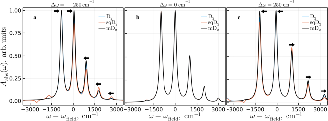
Figure 1: Absorption spectrum of a monomer ($\mathcal{M}_{1}$ model) at 300 K temperature with $\Delta\omega_{1,1}$ equal to a) $-250\ \text{cm}^{-1}$, b) $0\ \text{cm}^{-1}$, c) $+250$ $\text{cm}^{-1}$ simulated using $\text{D}_{2},$ $\text{sqD}_{2}$ and $\text{mD}_{2}$ ansatze. Arrows indicate peak frequency shift direction when compared to the $\Delta\omega=0$ case.

We assume spontaneus emission to only occur from the lowest energy excited aggregate vibronic state. After initial excitation by an external field, due to non-radiative relaxation processes and interaction with an environment, during the sufficiently long waiting time, $\tau\to\infty$, aggregate relaxes towards the minimal energy $E_{0}^{(\text{e})}$ excited aggregate vibronic state, $|\Psi_{\text{E}_{0}}^{\left(\text{e}\right)}\left(\tau\right)\rangle$. From TRF response function in Eq. (17) now follows that the fluorescence response function can be written as

$$S_{\text{flor}}^{\left(1\right)}\left(t\right)=\langle\Psi_{\text{E}_{\text{0}}}^{\left(\text{e}\right)}\left(0\right)|e^{-i\hat{H}t}\hat{\mu}_{-}e^{-i\hat{H}_{\text{G}}t}\hat{\mu}_{-}|\Psi_{\text{E}_{0}}^{\left(\text{e}\right)}\left(0\right)\rangle,$$ (18)

where , for convenience, we set the long waiting time to $\tau=0$. Note, that Eq. (18) does not contain summation over thermal ensemble trajectories $\gamma$, as the the minimal energy $E_{0}^{(\text{e})}$ and initial state $|\Psi_{\text{E}_{0}}^{\left(\text{e}\right)}\left(0\right)\rangle$ does not depend on initial vibrational conditions (temperature), but is solely a function of Hamiltonian and chosen ansatz.

The lowest energy state $|\Psi_{E_{0}}^{\left(\text{e}\right)}\left(0\right)\rangle$ is obtained by numerical optimization of excited state energy. That is obtained using heuristic adaptive particle swarm optimization algorithm [34, 35] by minimizing the total aggregate energy $E=\langle\Psi|\hat{H}|\Psi\rangle$, as a function of respective ansatz free parameters. For a given model of interest, optimization has to be performed once and can be reused afterwards.

At finite temperature $T$, due to thermal energy fluctuations, the resulting thermal ensemble in the excited aggregate state has larger average energy $\left\langle E_{0}^{(\text{e})}\right\rangle_{T}\geq E_{0}^{(\text{e})}$. Therefore, after waiting time $\tau$ aggregate can be in any one of the thermal ensemble states. Now fluorescence response function $S_{\text{flor}}^{\left(1\right)}\left(t\right)$ is obtained by averaging over an ensemble of thermal excited states $|\Psi_{\text{E}_{T}}^{\left(\text{e}\right)}\left(0\right)\rangle_{\gamma}$, where $\gamma$ is a trajectory number.

In order to find $|\Psi_{\text{E}_{T}}^{\left(\text{e}\right)}\left(0\right)\rangle_{\gamma}$ states, we cannot use the same algorithm as for the electronic ground state since all vibrational modes in electronic excited state are now indirectly coupled. Additionally, their frequencies are shifted if the quadratic vibronic coupling contributes.

For each trajectory $\gamma$, thermal excited states $|\Psi_{\text{E}_{T}}^{\left(\text{e}\right)}\left(0\right)\rangle_{\gamma}$ is obtained by perturbing $|\Psi_{\text{E}_{0}}^{\left(\text{e}\right)}\left(0\right)\rangle$ free parameters in such a way as to increase its total energy by the energy fluctuation $\delta E_{\gamma}=\sum_{n,q}\omega_{nq}^{\left(\text{e}\right)}\left|\tilde{\lambda}_{nq}^{\left(\gamma\right)}\right|^{2}$, where $\tilde{\lambda}_{nq}^{\left(\gamma\right)}$ are sampled from the excited state $\mathcal{P}^{\left(\text{e}\right)}$ distribution in Eq. (12). In order to find free parameters that correspond to energy $E_{\gamma}=E_{0}^{(\text{e})}+\delta E_{\gamma}$, we perturb CS displacements $\lambda_{nq}\left(\tau\right)$ for $\text{D}_{2}$, $\text{sqD}_{2}$ ansatze and $\lambda_{i,nq}\left(\tau\right)$ for $\text{mD}_{2}$ ansatz, until the new state energy $E_{\gamma}^{\text{fit}}=\langle\Psi_{\text{E}_{T}}^{\left(\text{e}\right)}\left(0\right)|_{\gamma}\hat{H}|\Psi_{\text{E}_{T}}^{\left(\text{e}\right)}\left(0\right)\rangle_{\gamma}$ matches $E_{\gamma}$ with $0.1\ \text{cm}^{-1}$ precision. Fluorescence response function at finite temperature is then equal to

$$S_{\text{flor}}^{\left(1\right)}\left(t\right)=\frac{1}{\Gamma}\sum_{\gamma=1}^{\Gamma}\langle\Psi_{\text{E}_{T}}^{\left(\text{e}\right)}\left(0\right)|_{\gamma}e^{-i\hat{H}t}\hat{\mu}_{-}e^{-i\hat{H}_{\text{G}}t}\hat{\mu}_{-}|\Psi_{\text{E}_{T}}^{\left(\text{e}\right)}\left(0\right)\rangle_{\gamma}.$$ (19)

III Results

III.1 Model parameters

In this section we investigate effects of intermolecular coupling and vibrational mode frequency shifts in Eq. (5), on absorption and fluorescence spectra. We consider three models. First model, $\mathcal{M}_{1}$, contains a single pigment coupled to one high frequency intramolecular mode. Second, $\mathcal{M}_{2}$, is a J-type dimer of two coupled chromophores, where excitations are coupled to a single high frequency intramolecular vibrational mode (one per pigment). Third, $\mathcal{M}_{3}$, is again two chromophore system, but here electronic excitations are coupled to overdamped phonon bath.

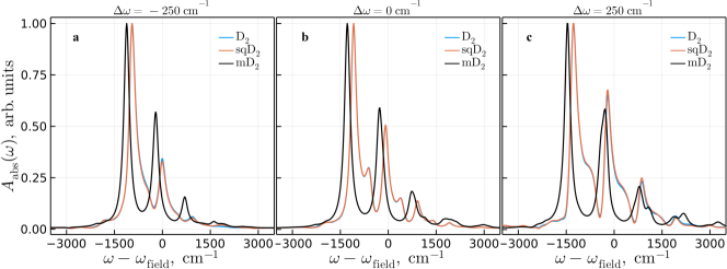
Figure 2: Absorption spectrum of a J-type dimer ($\mathcal{M}_{2}$ model) at 300 K temperature with $\Delta\omega_{1,1}=\Delta\omega_{2,1,}$ equal to a) $-250\ \text{cm}^{-1}$, b) $0\ \text{cm}^{-1}$, c) $+250$ $\text{cm}^{-1}$ simulated using $\text{D}_{2},$ $\text{sqD}_{2}$ and $\text{mD}_{2}$ ansatze.

The J-type dimers in models $\mathcal{M}_{2}$ and $\mathcal{M}_{3}$ consist of two pigments, each of which can be resonantly excited by an external electric field, thus we assume that single pigment excitation energies are resonant with optical field, $\varepsilon_{n}=\omega_{\text{field}}$, where $\omega_{\text{field}}$ is an external field frequency. Electronic transition dipole moment vectors of the chromophores are identical, $\boldsymbol{\mu}_{n}=\left(1,0,0\right)$, in Cartesian coordinate system. For $\mathcal{M}_{1}$ model, intramolecular vibrational mode frequency in the electronic ground state is $\omega_{1,1}^{g}=1000\ \text{cm}^{-1}$ and Huang-Rhys (HR) factor is $S=f_{1,1}^{2}=1$. For $\mathcal{M}_{2}$ model, the resonance coupling is $J_{12}=-500\ \text{cm}^{-1}$, while vibrational mode frequencies of the chromophores are $\omega_{1,1}^{g}=\omega_{2,1}^{g}=1000\ \text{cm}^{-1}$ with HR factors $S=f_{1,1}^{2}=f_{2,1}^{2}=1$. For $\mathcal{M}_{3}$ model, the resonance coupling is $J_{12}=-50\ \text{cm}^{-1}$ and vibrational phonon mode frequencies $\omega_{n,q}^{g}$ span from $0.1\ \text{cm}^{-1}$ to $490.1\ \text{cm}^{-1}$ with step-size of $10\ \text{cm}^{-1}$ for each pigment $n$ to represent overdamped phonon bath with a given spectral density. Here the $f_{nq}$ distribution is defined in terms of discretized quasi-continuos spectral density function

$$C_{n}^{"}\left(\omega\right)=\pi\sum_{q}f_{nq}^{2}\omega_{nq}^{e}\delta(\omega-\omega_{n,q}),$$ (20)

where $C_{n}^{"}\left(\omega\right)=\omega/\left(\omega^{2}+\gamma^{2}\right)$ is the Drude function with damping $\gamma=100\ \text{cm}^{-1}$. Magnitudes of $f_{nq}$ are then normalized so that the total reorganization energy $\Lambda_{n}=100\ \text{cm}^{-1}$ for each pigment $n$.

Models $\mathcal{M}_{1}$ and $\mathcal{M}_{2}$ are typically found in synthetic pigment aggregates [36, 37, 38], while $\mathcal{M}_{3}$ model more closely corresponds to chlorophyl aggregates found in nature [3, 1].

When plotting the simulated absorption and fluorescence response functions according to the Eq. (13), we will include phenomenological dephasing rate of $\gamma_{\text{dep}}=50\ \text{fs}$ for models $\mathcal{M}_{1}$, $\mathcal{M}_{2}$ and rate of $\gamma_{\text{dep}}=250\ \text{fs}$ for model $\mathcal{M}_{3}$. These are to account for additional dephasing stemming from explicitly not included phonons (for models $\mathcal{M}_{1}$, $\mathcal{M}_{2}$) and chromophone vibrational modes (for model $\mathcal{M}_{3}$).

III.2 Absorption spectra

In all models, we vary vibrational mode frequencies in the excited state $\omega_{nq}^{e}$ by shifting them from frequencies in the ground state $\omega_{nq}^{g}$, thus we define the difference of frequencies as $\Delta\omega_{nq}=\omega_{nq}^{e}-\omega_{nq}^{g}$. First, we start by investigating absorption spectrum of $\mathcal{M}_{1}$ model. In Fig. (1) we present absorption spectrum of the monomer at 300 K temperature with frequency shifts of $\Delta\omega_{1,1}\equiv\Delta\omega=-250,\ 0,\ +250\ \text{cm}^{-1}$. .

When $\Delta\omega=0$, we observe absorption spectrum with vibrational peak progresion representing jumps from ground to an arbitrary vibrational excited state. All three ansatze produce identical spectra since there is no electronic coupling and the nonlinear effects, due to quadratic vibronic coupling, are also absent. Now, when vibrational mode frequency in the excited state is higher than the ground state ($\Delta\omega=250\ \text{cm}^{-1}$), nonlinear effects become evident together with non-physical features in spectra of some ansatze. Absorption spectra of $\text{D}_{2}$ and $\text{sqD}_{2}$ ansatz have a negative peak at $\approx 2000\ \text{cm}^{-1}$ suggesting that they are unable to fully capture the nonlinear effects, i.e., they are not exact solutions of the Schrödinger equation. Meanwhile, $\text{mD}_{2}$ ansatz with $M=5$ superposition terms produce strictly positive absorption spectra and thus will be considered to be the reference spectra for further comparisons. To check validity of this claim, we compared $\text{mD}_{2}$ spectra simulated with $M=1-10$ terms and found $M\geq 5$ spectra to be quantitatively exact (not shown). Besides the negative peaks, neither $\text{D}_{2}$ nor $\text{sqD}_{2}$ are able to reproduce vibrational peak progression amplitudes of $\text{mD}_{2}$ ansatz.

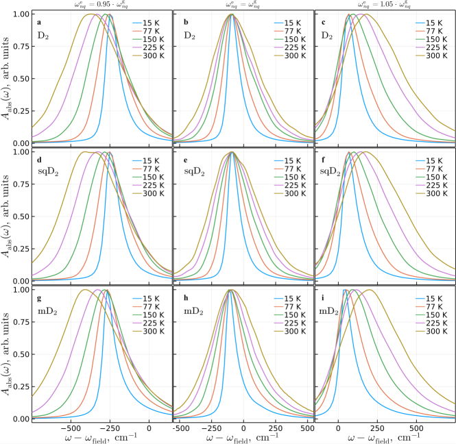
Figure 3: Absorption spectrum of a J dimer ($\mathcal{M}_{3}$ model) coupled to the phonon bath at various temperatures with vibrational mode frequencies in aggregate excited states $\omega_{nq}^{e}$ equal to a) $0.95\cdot\omega_{nq}^{g}$, b) $\omega_{nq}^{g}$, c) $1.05\cdot\omega_{nq}^{g}$ simulated using $\text{D}_{2}$ (1st row), $\text{sqD}_{2}$ (2nd row) and $\text{mD}_{2}$ (3rd row) ansatze.

By comparing $\text{mD}_{2}$ absorption spectra peak amplitude progression in all three $\Delta\omega$ cases, we find that progression peak amplitudes either increase or are reduced as compared to the $\Delta\omega=0$ spectrum, we will refer to these qualitative changes as model having increased or decreased effective HR factor. Therefore, effective HR is reduced when $\Delta\omega$ is positive, and is increased when $\Delta\omega$ is negative. In addition, $\Delta\omega$ also changes progression peak frequencies, however, not in a monotonic fashion. Direction of frequency change of each peak is indicated by an arrow, when compared to the $\Delta\omega=0$ case. Absolute frequency of some peaks increase, while for others it decreases. This can also be interpreted as relative energy gap between progression peaks becoming larger when $\Delta\omega$ is positive, and gap is reduced when $\Delta\omega$ is negative.

Next, we look at absorption spectrum of model $\mathcal{M}_{2}$. In Fig. (2) we present absorption spectrum of the J dimer at 300 K temperature with shifts $\Delta\omega_{1,1}=\Delta\omega_{2,1,}\equiv\Delta\omega=-250,\ 0,\ 250\ \text{cm}^{-1}$. Now, even in the $\Delta\omega=0$ case, when nonlinear effects are still absent, we find mismatch between absorption spectrum simulated using $\text{D}_{2},\text{sqD}_{2}$ ansatze and $\text{mD}_{2}$. This is purelly due to electronic coupling between vibronic states of sites, which was lacking in model $\mathcal{M}_{1}$. Also, notice that spectra of $\text{D}_{2}$, $\text{sqD}_{2}$ ansatze are identical, since according equations $\text{sqD}_{2}$ becomes different from $\text{D}_{2}$ only when quadratic vibronic coupling is present, i.e. $\Delta\omega\neq 0$. The exact $\text{mD}_{2}$ spectrum has a familiar J dimer absorption lineshape dominated by the exchange narrowing effect [39], which effectively reduces HR factor as compared to the monomer in Fig. (1). Absorption spectra of $\text{D}_{2}$, $\text{sqD}_{2}$ ansatze reproduces exchange narrowing effect, however, their spectra has additional secondary peaks not seen in $\text{mD}_{2}$ spectrum. Their spectra also has slightly higher energy 0-0 quanta transitions peak (and 0-1, 0-2, etc.) as compared to the $\text{mD}_{2}$ spectrum, which implies that $\text{mD}_{2}$ is able to better represent lower energy excited aggregate state.

When the quadratic vibronic coupling effects are present ($\Delta\omega=-250,\ 250\ \text{cm}^{-1}$), again, in both cases, we find $\text{D}_{2},\text{sqD}_{2}$ spectra to differ from $\text{mD}_{2}$ spectra. Very slight differences can also be seen between $\text{D}_{2}$ and $\text{sqD}_{2}$ ansatze, however, without any obvious improvement from $\text{sqD}_{2}$. In both cases, $\text{mD}_{2}$ spectra again shows J dimer exchange narrowing type lineshape with changes to peak amplitudes similar to those seen in Fig. (1) – relative energy gap between peaks become larger when $\Delta\omega$ is positive, and is reduced when $\Delta\omega$ is negative. Spectrum with $\Delta\omega=250\ \text{cm}^{-1}$ has a more pronounced fine structure to its absorption progression peaks than those spectra with $\Delta\omega=-250\ \text{cm}^{-1}$ and $=0$.

These findings suggest that neither $\text{D}_{2}$ nor a more complicated $\text{sqD}_{2}$ are able to fully capture absorption spectrum of J dimers with high frequency intramolecular vibrational modes, not even in the simplest case ($\Delta\omega=0\ \text{cm}^{-1}$) when the quadratic vibronic coupling is excluded..

Next, lets look at the absorption spectra of $\mathcal{M}_{3}$ model. In this case phonon modes become thermally excited so we additionally present temperature-dependent spectra. In Fig. (3) we present absorption spectra of a J dimer coupled to phonon bath at various temperatures. Now each chromophone couples to 50 low frequency vibrational modes, therefore, to investigate quadratic vibronic coupling effect, we will look at cases when all modes’ frequencies, $\omega_{nq}^{e}$, in an excited aggregate are equal to frequencies in an ground aggregate state, $\omega_{nq}^{g}$, scaled by a factor of $\gamma=0.95,\ 1,\ 1.05$.

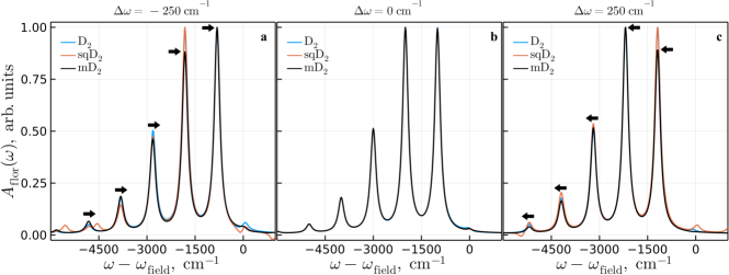
Figure 4: Fluorescence spectrum of a monomer ($\mathcal{M}_{1}$ model) at 300 K temperature with $\Delta\omega_{1,1}$ equal to a) $-250\ \text{cm}^{-1}$, b) $0\ \text{cm}^{-1}$, c) $+250$ $\text{cm}^{-1}$ simulated using $\text{D}_{2},$ $\text{sqD}_{2}$ and $\text{mD}_{2}$ ansatze. Arrows indicate peak frequency shift direction when compared to the $\Delta\omega=0$ case.

When $\gamma=1$, all methods produce qualitatively identical absorption spectra over a broad range of temperatures. At low temperatures spectra consists of a single absorption peak. With increasing temperature, spectra broadens and slightly shifts (on average) due to thermal excitation of vibrational modes in electronic ground state and due to finite discretization at low frequencies. .

Now, when phonon mode frequencies in the aggregate excited state are higher ($\gamma=1.05$), in addition to the previously seen thermal spectra broadening, we also observe two type of spectral shifts: a static shift – the whole absorption spectra shifts to the higher energies, as compared to the $\gamma=1$ case, and a temperature dependent absorption peak shift to the higher energies. Spectra simulated with all ansatze when $\gamma=1.05$ are also qualitativelly similar, however, spectrum of $\text{mD}_{2}$ in Fig. (3i) has a less straightforward temperature dependent peak shift dependence. Peak frequency changes not as linearly with temperature as in spectra simulated with $\text{D}_{2}$ and $\text{sqD}_{2}$ ansatze in Fig. (3c) and Fig. (3f). Similarly, when phonon mode frequencies in the aggregate excited state are lower ($\gamma=0.95$), we find all the same spectral shift effects, only now to the lower energy side.Spectra simulated with different ansatze appear qualitatively the same, therefore we conclude that to simulate absorption spectra of J dimer coupled to low frequency phonon modes, even with quadratic vibronic coupling, it is sufficient to use the simplest $\text{D}_{2}$ ansatz.Fluorescence spectra

$\mathcal{M}_{1}$	$\Delta\omega$	$\text{D}_{2}$	$\text{sqD}_{2}$	$\text{mD}_{2}$
	$-250$	-812.5	-812.5	-816.9
	0	-1000.0	-1000.0	-1000.0
	$250$	-1187.5	-1190.9	-1190.9
$\mathcal{M}_{2}$	$\Delta\omega$	$\text{D}_{2}$	$\text{sqD}_{2}$	$\text{mD}_{2}$
	$-250$	-956.3	-959.9	-1119.2
	$0$	-1125.0	-1125.0	-1284.7
	$250$	-1131.9	-1302.0	-1460.9
$\mathcal{M}_{3}$	$\omega_{nq}^{e}$	$\text{D}_{2}$	$\text{sqD}_{2}$	$\text{mD}_{2}$
	$0.95\cdot\omega_{nq}^{g}$	-265.09	-265.1	-265.0
	$1.0\cdot\omega_{nq}^{g}$	-112.5	-112.2	-111.7
	$1.05\cdot\omega_{nq}^{g}$	41.1	40.4	41.1

Table 1: Energy $E_{0}^{(\text{e})}$ of aggregate excited state $|\Psi_{\text{E}_{0}}^{\left(\text{e}\right)}\left(0\right)\rangle$ for models $\mathcal{M}$ using $\text{D}_{2}$, $\text{sqD}_{2}$ and $\text{mD}_{2}$ ansatze. $\text{mD}_{2}$ ansatz consist of $M=5$ superposition terms. Values are in units of $\text{cm}^{-1}$.

In order to compute fluorescence spectrum, for each considered ansatze, we first have to find the lowest energy $E_{0}^{(\text{e})}$ excited aggregate state $|\Psi_{E_{0}}^{\left(\text{e}\right)}\left(0\right)\rangle$ in terms of that ansatz free parameter by minimizing the total aggregate energy $E=\langle\Psi|\hat{H}|\Psi\rangle$, as explained in Section (II.2). The resulting energies $E_{0}^{(\text{e})}$ for models $\mathcal{M}$ are given in Table (1).

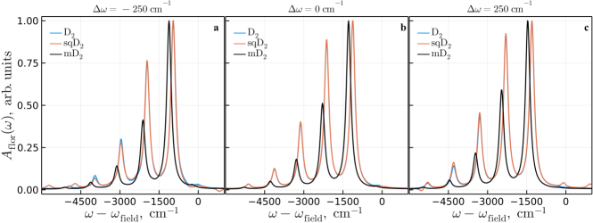
Figure 5: Fluorescence spectrum of a J dimer ($\mathcal{M}_{2}$ model) at 300 K temperature with $\Delta\omega_{1,1}=\Delta\omega_{2,1,}$ equal to a) $-250\ \text{cm}^{-1}$, b) $0\ \text{cm}^{-1}$, c) $250$ $\text{cm}^{-1}$ simulated using $\text{D}_{2},$ $\text{sqD}_{2}$ and $\text{mD}_{2}$ ansatze.

We see that for model $\mathcal{M}_{1}$, when vibrational nonlinearities are absent, all ansatze give exactly the same energy, however, by including the quadratic vibronic coupling ($\Delta\omega\neq 0$ cases), both $\text{sqD}_{2}$ and $\text{mD}_{2}$ find lower energy states than $\text{D}_{2}$ ansatz. $\text{mD}_{2}$ ansatz further outperform $\text{sqD}_{2}$ ansatz, when $\Delta\omega$ is negative. Consequently, $\text{sqD}_{2}$ model outperforms $\text{D}_{2}$ ansatz when searching for excited state energy minimum when quadratic coupling is included.

In model $\mathcal{M}_{2}$, when $\Delta\omega=0$, we see that $\text{D}_{2}$ and $\text{sqD}_{2}$ again find equivalent energy state, however, now $\text{mD}_{2}$ ansatz manages to represent significantly lower energy state, which is not accessed by any of the non-multiple ansatze and is created purelly due to electronic coupling between pigments. When nonlinearities are included, $\text{sqD}_{2}$ ansatz again outperforms $\text{D}_{2}$, especially when $\Delta\omega$ is positive, yet $\text{mD}_{2}$ further improves on $\text{sqD}_{2}$ states.

In model $\mathcal{M}_{3}$, we try to find minimum point in 1020-dimensional space for $\text{mD}_{2}$, 204-dimensional for $\text{D}_{2}$, and 404-dimensional for $\text{sqD}_{2}$, which is a difficult problem to solve. To have a fair comparison of ansatze for model $\mathcal{M}_{3}$, we limited search for the state $|\Psi_{E_{0}}^{\left(\text{e}\right)}\left(0\right)\rangle$ in terms of $\text{sqD}_{2}$ ansatz to its sqCS displacement parameters, $\lambda_{kq}$, and set squeezing parameters to $r_{kq}=1$, $\theta_{kq}=0$ (no squeezing). For the $\text{mD}_{2}$ ansatz, we limited search to just one of its multiples. With these limits set, essentially both $\text{sqD}_{2}$ and $\text{mD}_{2}$ ansatz behave as $\text{D}_{2}$, thus all three ansatze relax to the same excited aggregate state with energies equivalent to those under $\text{D}_{2}$ column. This is confirmed by numberical results where all ansatze managed to represent states with very similar energies. The obtained numbers are also likely within the margin of error and require an improved approach for finding actual lowest energy states.

Now, lets look at fluorescence spectra of the same $\mathcal{M}$ models. In Fig. (4) we display fluorescence spectra of a monomer coupled to high frequency vibration ($\mathcal{M}_{1}$ model) at 300 K temperature with frequency shifts of $\Delta\omega_{1,1}\equiv\Delta\omega=-250,\ 0,\ +250\ \text{cm}^{-1}$. When $\Delta\omega=0$, we find all three ansatze to produce identical fluorescence spectra, which, as expected, has a mirror symmetry with $\mathcal{M}_{1}$ model absorption spectrum in Fig. (1b). Fluorescence spectrum consists of progression of energeticaly downward transition peaks.

When the quadratic vibronic coupling term is included ($\Delta\omega=-250,\ +250\ \text{cm}^{-1}$), simulated fluorescence spectra of considered ansatze are different. In both cases, fluorescence spectrum of $\text{D}_{2}$ qualitatively match $\text{mD}_{2}$ ansatz spectrum peak amplitudes and frequencies, while the intermediate complexity $\text{sqD}_{2}$ consistently overestimate peak amplitudes and show additional peaks that are not present in $\text{mD}_{2}$ ansatz spectrum. Here we see an example, where additional, but not sufficient, DOF (squeezing) of $\text{sqD}_{2}$ ansatz actually produce visually worse quality spectrum than the smaller state space $\text{D}_{2}$ ansatz. This is in contrast to absorption spectra of $\mathcal{M}_{1}$ model, where both $\text{D}_{2}$ and $\text{sqD}_{2}$ ansatz showed equivalent errors when compared to $\text{mD}_{2}$ spectra.

By comparing $\text{mD}_{2}$ fluorescence spectra with quadratic vibronic coupling to that without it, we find that fluorescence progression peak amplitudes change – effective HR factor increases when $\Delta\omega$ is positive, and decreases when $\Delta\omega$ is negative. Also, quadratic vibronic coupling shifts whole spectra to the lower energy side when $\Delta\omega$ is positive, and to the higher side when $\Delta\omega$ is negative. In contrast to the absorption spectra in Fig. (1), energy gaps between progression peaks remain unchanged, Also, by comparing quadratic vibronic coupling absorption and fluoresnce spectra of $\mathcal{M}_{1}$ model of $\text{mD}_{2}$ ansatz, we see that quadratic vibronic coupling breaks the mirror symmetry between the two.

Now, lets move on to the $\mathcal{M}_{2}$ model. In Fig. (5) we show its fluorescence spectrum simulated at 300 K temperature with $\Delta\omega_{1,1}=\Delta\omega_{2,1,}\equiv\Delta\omega$ equal to $-250\ \text{cm}^{-1}$, $0\ \text{cm}^{-1}$, $250$ $\text{cm}^{-1}$.

When nonlinearities are absent ($\Delta\omega=0$), we again see that $\text{D}_{2}$ and $\text{sqD}_{2}$ ansatze yeld identical fluorescence spectra, which differ from the spectrum of $\text{mD}_{2}$ ansatz in fluorescence peak amplitudes and frequencies. The discrepency between spectra is again a result of $\text{D}_{2}$, $\text{sqD}_{2}$ ansatze not being able to properly represent vibronic states created by electronic coupling between J dimer pigments. The lineshape of $\text{mD}_{2}$ fluorescence spectrum is dominated by the exchange narrowing effect and does not have mirror symmetry with absorption spectrum.

From fluorescence spectra of $\mathcal{M}_{2}$ model with the quadratic vibronic coupling term ($\Delta\omega=-250,\ +250\ \text{cm}^{-1}$), we draw the same conclusions as in the $\mathcal{M}_{1}$ model: $\text{D}_{2}$ spectrum matches $\text{mD}_{2}$ spectrum better than does $\text{sqD}_{2}$; effective HR factor increases when $\Delta\omega$ is positive, and decreases when $\Delta\omega$ is negative; quadratic vibronic coupling shift spectra to the lower energy side when $\Delta\omega$ is positive, and to the higher side when $\Delta\omega$ is negative; energy gaps between progression peaks remain unchanged from $\Delta\omega=0$ spectrum.

Overall, fluorescence spectrum of J dimer coupled to the high frequency vibrational modes is accuratelly captured only by the $\text{mD}_{2}$ ansatz, while $\text{sqD}_{2}$ yield visually slightly worse quality spectrum than that of $\text{D}_{2}$ ansatz, however, neither are to match $\text{mD}_{2}$ accuracy.

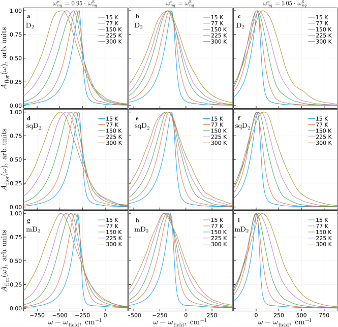
Figure 6: Fluorescence spectrum of a J dimer ($\mathcal{M}_{3}$ model) coupled to the bath at various temperatures with vibrational mode frequencies in aggregate excited states $\omega_{nq}^{e}$ equal to a) $0.95\cdot\omega_{nq}^{g}$, b) $\omega_{nq}^{g}$, c) $1.05\cdot\omega_{nq}^{g}$ simulated using $\text{D}_{2}$ (1st row), $\text{sqD}_{2}$ (2nd row) and $\text{mD}_{2}$ (3rd row) ansatze.

Next, lets look at the fluorescence spectra of $\mathcal{M}_{3}$ model. In Fig. (6) we show fluorescence spectra of a J dimer coupled to bath of low frequency phonon modes at various temperatures. We see that all ansatze produce qualitatively simillar fluorescence spectra with all vibrational mode scalling factors $\gamma=0.95,\ 1,\ 1.05$. As in absorption spectra of $\mathcal{M}_{3}$ model in Fig. (3), we find analogous effects of spectral broadening with increasing temperature, as well as two type of spectral shifts: a static shift – the whole spectrum shifts to the higher energies when $\gamma$ is positive, and to the lower energies when $\gamma$ is negative, as compared to the $\gamma=1$ case, and an additional temperature dependent fluorescence peak shift to the higher energy side when $\gamma$ is positive, and to the lower side when $\gamma$ is negative. In addition to these, we now observe fluorescence peak drift to the lower energies with increasing temperature when the frequency scale factor is $\gamma=1$, regardless of the ansatze used.

All in all, spectra simulated with considered ansatze appear qualitatively equivalent, thus we conclude that to simulate fluorescence spectra of J dimer coupled to low frequency phonon modes, even with quadratic vibronic coupling, it is sufficient to use the simplest $\text{D}_{2}$ ansatz.

IV Discussion

Natural progression in constructing more and more sophisticated Davydov type ansatze, would be to write down ansatz as a superposition of $\text{sqD}_{2}$ ansatze – the $\text{multi-sqD}_{2}$ ansatz. This was recently done by Zeng et al. [40], where they used it to simulate dynamics and absorption spectra of pyrazine and the 2-pyridone dimer aggregate, and found a great match with the state-of-the-art multi-configuration time-dependent Hartree (MCTDH) method results. In fact, presented approach of using Davydov type ansatze is closely related to the Gaussian-MCTDH with frozen Gaussians functions for $\text{D}_{2}$, $\text{mD}_{2}$ ansatze, and $\text{sqD}_{2}$ with thawed Gaussian functions [6, 41, 42, 43].

Our analysis presented in Section (III), show that using sqCS, instead of regular CS, does not provide any significant improvement to the simulated absorption and fluorescence spectra of J dimers, even when the quadratic vibronic coupling is used. Therefore one has to wonder if an additional numerical effort needed to propagate $\text{multi-sqD}_{2}$ ansatz is worth, since any arbitrary wavefunction can be already exactly expanded using $\text{mD}_{2}$ ansatz using the unity operator expression

$$\hat{I}=\pi^{-1}\iint\text{d\text{Re}{\hbox{\lambda}}}\ \text{d\text{Im}{\hbox{\lambda}}}\ |\lambda\rangle\langle\lambda|.$$ (21)

It would be interesting to see if the $\text{multi-sqD}_{2}$ ansatz would require less terms in its superposition than the $\text{mD}_{2}$ ansatz to obtain equivalent spectra. However, this is outside the topic of this paper.

We looked at the quadratic vibronic coupling effects for low and high frequency modes. For the high frequency modes, we looked at large nonlinearities by increasing and decreasing mode frequency by 25%, which is much larger than what is observed in molecules [14]. This was chosen to investigate limits of all ansatze, however, for smaller nonlinearities we expect the same conclusion, i.e., that multiple-type ansatze are required to simulate aggregate spectra. This is because we considered strong electronic coupling between pigments, which eventually splits wavepacket into several discrete packets and move quasi-independent along seperate vibronic state energy surfaces, while the quadratic vibronic coupling introduces only the secondary effects, which were not captured by non-multiple ansatze.

For the low frequency modes, we considered small nonlinearities by changing frequencies by 5%, more in line with what is observed, with small electronic coupling between pigments, and found all considered ansatze to produce qualitativelly identical spectra. This implies that even when quadratic vibronic coupling is the main source of nonlinearity, for realistic frequency shifts, sqCS does not provide any significant improvement. However, it is worth mentioning that $\text{sqD}_{2}$ model outperforms $\text{D}_{2}$ ansatz when searching for excited state energy minimum when quadratic coupling is included. This improvement may be important for other types of processes such as charge separation and internal conversion.

In conclusion, we compared absorption and fluorescence spectra of vibronic J dimer model with quadratic vibronic coupling simulated using three increasing sophistication wavefunction ansatze: $\text{D}_{2}$, $\text{sqD}_{2}$ and $\text{mD}_{2}$. We found that it is necessary to use $\text{mD}_{2}$ ansatz whenever molecular aggregate electronic DOFs are coupled to higher frequency intramolecular vibrational modes. If they are coupled to low frequency phonon bath modes, all three ansatze produce qualitatively the same spectra. The quadratic vibronic coupling term manifests itself in both absorption and fluorescence spectra as a lineshape peak amplitude redistribution, static frequency shift and an additional shift, which is dependent on the temperature.

Conflicts of interest

There are no conflicts of interest to declare.

Appendix A Time-dependent variational principle

Will be using time-dependent Dirac-Frenkel variational principle to obtain a set of equations of motion of the $\text{D}_{2},\text{sqD}_{2}$ and $\text{mD}_{2}$ ansatze free parameters: $\Gamma_{\text{D}_{2}}=\left\{\alpha_{n}\left(t\right),\lambda_{kq}\left(t\right)\right\}$, $\Gamma_{\text{sqD}_{2}}=\left\{\alpha_{n}\left(t\right),\lambda_{kq}\left(t\right),r_{kq}\left(t\right)\right\}$ and $\Gamma_{\text{mD}_{2}}=\left\{\alpha_{i,n}\left(t\right),\lambda_{i,kq}\left(t\right)\right\}$. Solution of the set of equations will result in ansatze time evolution, such that the deviation from an exact solution of the Schrödinger equation will be minimized. As a first step, we write down model Lagrangian in the form of

$$\mathcal{L}\left(t\right) =\frac{\text{i}}{2}\left(\langle\Psi\left(t\right)|\dot{\Psi}\left(t\right)\rangle-\langle\dot{\Psi}\left(t\right)|\Psi\left(t\right)\rangle\right)$$

$$-\langle\Psi\left(t\right)|\hat{H}|\Psi\left(t\right)\rangle$$ (22)

where $\dot{x}\left(t\right)$ is the time derivative of $x\left(t\right)$. For the $\text{sqD}_{2}$ ansatz, Lagrangian can be expressed as (hereafter, we omit explicitly writing parameter time dependence)

$$\mathcal{L}_{\text{sqD}_{2}} =\frac{\text{i}}{2}\sum_{n}\alpha_{n}^{*}\dot{\alpha}_{n}-\frac{\mathrm{i}}{2}\sum_{m}\alpha_{m}\dot{\alpha}_{m}^{*}$$

$$+\frac{\text{i}}{2}\sum_{n,h,q}\left|\alpha_{n}\right|^{2}\left(\dot{\lambda}_{hq}\lambda_{hq}^{*}-\dot{\lambda}_{hq}^{*}\lambda_{hq}+\text{i}\dot{\theta}_{hq}\sinh^{2}\left(r_{hq}\right)\right)$$

$$-\sum_{n}\left|\alpha_{n}\right|^{2}\varepsilon_{n}-\sum_{n,m}^{n\neq m}V_{nm}\alpha_{m}\alpha_{n}^{*}$$

$$-\sum_{n,m,q}\left|\alpha_{m}\right|^{2}\omega_{nq}^{g}\left(\sinh^{2}\left(r_{nq}\right)+\left|\lambda_{nq}\right|^{2}\right)$$

$$+2\sum_{n,q}\left|\alpha_{n}\right|^{2}\omega_{nq}^{e}f_{nq}\text{Re}\lambda_{nq}$$

$$-\sum_{n,q}\left|\alpha_{n}\right|^{2}\Delta\omega_{nq}$$

$$\times \left(\cosh\left(2r_{nq}\right)-\sinh\left(2r_{nq}\right)\cos\left(\theta_{nq}\right)+\left(2\text{Re}\lambda_{nq}\right)^{2}\right)\ ,$$ (23)

and for the $\text{mD}_{2}$, Lagrangian reads

$$\mathcal{L}_{\text{mD}_{2}} =\text{i}\sum_{i,j}\sum_{n}\alpha_{i,n}^{\star}\dot{\alpha}_{j,n}S_{ij}$$

$$+\text{i}\sum_{i,j}\sum_{n}\alpha_{i,n}^{\star}\alpha_{j,n}S_{ij}K_{ij}$$

$$-\sum_{i,j}\sum_{n}\alpha_{i,n}^{\star}\alpha_{j,n}S_{ij}\varepsilon_{n}-\sum_{i,j}\sum_{n,m}\alpha_{i,n}^{\star}\alpha_{j,m}S_{ij}J_{nm}$$

$$-\sum_{ij}\sum_{n}\alpha_{i,n}^{\star}\alpha_{j,n}S_{ij}\sum_{h}\omega_{nh}\lambda_{i,nh}^{\star}\lambda_{j,nh}$$

$$+\sum_{ij}\sum_{n}\alpha_{i,n}^{\star}\alpha_{j,n}S_{ij}\sum_{h}\omega_{nh}f_{nh}\left(\tilde{\lambda}_{i,nh}^{\star}+\tilde{\lambda}_{j,nh}\right)$$

$$-\sum_{ij}\sum_{n}\alpha_{i,n}^{\star}\alpha_{j,n}S_{ij}\sum_{h}\Delta\omega_{nh}\left(1+\left(\lambda_{i,nh}^{\star}+\lambda_{j,nh}\right)^{2}\right),$$ (24)

where Debay-Waller factor is

$$S_{ij}= \exp\left\{\sum_{k,q}\lambda_{i,kq}^{\star}\lambda_{j,kq}-\frac{1}{2}\left(\left|\lambda_{i,kq}\right|^{2}+\left|\lambda_{j,kq}\right|^{2}\right)\right\},$$ (25)

and

$$K_{ij}=\sum_{kq}\lambda_{i,kq}^{\star}\dot{\lambda}_{j,kq}-\frac{1}{2}\frac{\text{d}}{\text{dt}}\left|\lambda_{j,kq}\right|^{2}.$$ (26)

Now, for each Lagrangian $\mathcal{L}_{\beta}$, where $\beta=\text{sqD}_{2},\ \text{mD}_{2}$, we applying the Euler-Lagrange equation

$$\frac{\text{d}}{\text{dt}}\left(\frac{\partial\mathcal{L}_{\beta}}{\partial\dot{\gamma_{\beta}}^{\star}}\right)-\frac{\partial\mathcal{L}_{\beta}}{\partial\gamma_{\beta}^{\star}}=0,$$ (27)

to each free parameters $\gamma_{\beta}\in\Gamma_{\beta}$ of ansatz in order to obtain equation of motion.

For the $\text{sqD}_{2}$ ansatz, this procedure results in a system of differential equations:

$$\dot{\alpha}_{n}= -\frac{1}{2}\alpha_{n}\sum_{h,q}\left(\dot{\lambda}_{hq}\lambda_{hq}^{*}-\dot{\lambda}_{hq}^{*}\lambda_{hq}\right)$$

$$-\frac{\mathrm{i}}{2}\alpha_{n}\sum_{h,q}\dot{\theta}_{hq}\sinh^{2}\left(r_{hq}\right)$$

$$-\mathrm{i}\alpha_{n}\varepsilon_{n}-\mathrm{i}\sum_{m}^{n\neq m}V_{m}\alpha_{m}$$

$$-\mathrm{i}\alpha_{n}\sum_{m,q}\omega_{mq}^{g}\left(\sinh^{2}\left(r_{mq}\right)+\left|\lambda_{mq}\right|^{2}\right)$$

$$+\mathrm{i}2\alpha_{n}\sum_{q}\omega_{nq}^{e}f_{nq}\text{Re}\lambda_{nq}$$

$$-\mathrm{i}\alpha_{n}\sum_{q}\Delta\omega_{nq}\cosh\left(2r_{nq}\right)$$

$$+\mathrm{i}\alpha_{n}\sum_{q}\Delta\omega_{nq}\sinh\left(2r_{nq}\right)\cos\left(\theta_{nq}\right)+\left(2\text{Re}\lambda_{nq}\right)^{2},$$ (28)

for each index $n$, and

$$\dot{\lambda}_{kh} =-\mathrm{i}\omega_{kh}^{g}\lambda_{kh}+\frac{\text{$\mathrm{i}$}}{\rho}\left|\alpha_{k}\right|^{2}\omega_{kh}^{e}f_{kh}$$

$$-4\frac{\text{i}}{\rho}\left|\alpha_{k}\right|^{2}\Delta\omega_{kh}\text{Re}\lambda_{kh},$$ (29)

$$\dot{r}_{kh}=\frac{\text{2}}{\rho}\left|\alpha_{k}\right|^{2}\Delta\omega_{kh}\sin\left(\theta_{kh}\right),$$ (30)

$$\dot{\theta}_{kh} =-2\omega_{kh}^{g}$$

$$-4\frac{\left|\alpha_{k}\right|^{2}}{\rho}\Delta\omega_{kh}\left(1-\coth\left(2r_{kh}\right)\cos\left(\theta_{kh}\right)\right),$$ (31)

for each pair of $\left\{k,h\right\}$ indeces.

We denote $\rho=\sum_{n}\left|\alpha_{n}\right|^{2}$ as the total population. Only the last two terms $r_{kh}$, $\theta_{kh}$, which make up the complex squeezing parameter $\zeta=r_{kh}e^{\text{i$\theta_{kh}$}}$, depend on $\Delta w$. Now, if we look back at Hamiltonian terms Eq. (2-5), we see straightaway that only the quadratic vibronic term depends on $\Delta w$, thus squeezing is generated only by this term. Otherwise, if $\Delta w=0$, squeezing amplitude $r_{kh}$ becomes time independent, while squeezing angle $\theta_{kh}$ changes at a constant rate $-2\omega_{kh}^{g}$.

For the $\text{mD}_{2}$ ansatz, variational principle yields a system of implicit differential equations:

$$\sum_{j}\left(\dot{\alpha}_{j,n}S_{ij}+\alpha_{j,n}S_{ij}K_{ij}\right)$$

$$=-\text{i}\sum_{j,m}\alpha_{j,m}S_{ij}J_{nm}$$

$$-\text{i}\sum_{j}\alpha_{j,n}S_{ij}\left(A_{ij}+B_{ij,n}+C_{ij,n}\right),$$ (32)

for each pair of indices $\left\{i,n\right\}$, and

$$\sum_{j,n}\left(\alpha_{i,n}^{\star}\dot{\alpha}_{j,n}S_{ij}\lambda_{j,kh}+P_{ij,n}\dot{\lambda}_{j,kh}+P_{ij,n}\lambda_{j,kh}K_{ij}\right)$$

$$=-\text{i}\sum_{j,n,m}G_{ij,nm}\lambda_{j,kh}J_{nm}$$

$$-\text{i}\sum_{j,n}P_{ij,n}\lambda_{j,kh}\left(A_{ij}+B_{ij,n}+C_{ij,n}\right)$$

$$-\text{i}\sum_{j,n}P_{ij,n}\omega_{kh}^{g}\lambda_{j,kh}+\text{i}\sum_{j}P_{ij,k}f_{kh}\omega_{kh}^{e}$$

$$-2\text{i}\sum_{j}P_{ij,k}\Delta\omega_{kh}\left(\lambda_{i,kh}^{\star}+\lambda_{j,kh}\right),$$ (33)

for pair of $\left\{i,k,h\right\}$ indices, where we additionally defined

$$G_{ij,nm} =\alpha_{i,n}^{\star}\alpha_{j,m}S_{ij},$$ (34)

$$P_{ij,n} =G_{ij,nn},$$ (35)

$$A_{ij} =\sum_{k,q}\omega_{kh}^{g}\lambda_{i,kh}^{\star}\lambda_{j,kh},$$ (36)

$$B_{ij,n} =-\sum_{h}f_{nh}\omega_{nh}^{e}\left(\lambda_{i,nh}^{\star}+\lambda_{j,nh}\right),$$ (37)

$$C_{ij,n} =\sum_{h}\Delta\omega_{nh}\left(1+\left(\lambda_{i,nh}^{\star}+\lambda_{j,nh}\right)^{2}\right).$$ (38)

For the $\text{D}_{2}$ ansatz, we once again can explicitly compute equations of motions following TDVP, however, we do not have to, since $\text{D}_{2}$ ansatz is a simplified version of $\text{mD}_{2}$ ansatz, when multiplicity number is set to $M=1$.

Calculation of linear response functions $S_{\text{abs/flor}}^{\left(1\right)}$ requires evaluation of two distinct coherent states. In the case of $\text{D}_{2}$ and $\text{mD}_{2}$ ansatze, the overlap between two distinct $a$ and $b$ coherent state are given b

$$\langle\lambda_{a}|\lambda_{b}\rangle=\exp\left(\lambda_{a}^{\ast}\lambda_{b}-\frac{1}{2}\left(|\lambda_{a}|^{2}+|\lambda_{b}|^{2}\right)\right).$$ (39)

Meanwhile, overlap of two squeezed coherent states, as used in $\text{sqD}_{2}$ ansatz, is given by expression [13]

$$\langle\lambda_{a},\zeta_{a}|\lambda_{b},\zeta_{b}\rangle =\frac{1}{\sqrt{\zeta_{ab}}}\exp\left(-\frac{\left|\lambda_{a}\right|^{2}+\left|\lambda_{b}\right|^{2}}{2}\right)$$

$$\times\exp\left(\frac{\lambda_{a}^{*}\lambda_{b}}{\zeta_{ab}}+\frac{\lambda_{a}^{*2}}{2\zeta_{ab}}\eta_{ab}+\frac{\lambda_{b}^{2}}{2\zeta_{ab}}\eta_{ba}\right),$$ (40)

where

$$\eta_{ab} =e^{-\text{i}\theta_{b}}\cosh\left(r_{a}\right)\sinh\left(r_{b}\right)-e^{-\text{i}\theta_{a}}\cosh\left(r_{b}\right)\sinh\left(r_{a}\right),$$ (41)

$$\zeta_{ab} =\cosh\left(r_{a}\right)\cosh\left(r_{b}\right)-e^{\text{i}\left(\theta_{b}-\theta_{a}\right)}\sinh\left(r_{a}\right)\sinh\left(r_{b}\right).$$ (42)

References

- Valkunas et al. [2013] L. Valkunas, D. Abramavicius and T. Mančal, Molecular Excitation Dynamics and Relaxation, Wiley-VCH Verlag GmbH, 2013.
- Blankenship [2002] R. E. Blankenship, Molecular Mechanisms of Photosynthesis, Blackwell Science Ltd, Oxford, UK, 2002.
- van Amerongen et al. [2000] H. van Amerongen, R. van Grondelle and L. Valkunas, Photosynthetic Excitons, World Scientific, 2000.
- Davydov [1979] A. S. Davydov, Physica Scripta, 1979, 20, 387–394.
- Scott [1991] A. C. Scott, Physica D: Nonlinear Phenomena, 1991, 51, 333–342.
- Zhao et al. [2022] Y. Zhao, K. Sun, L. Chen and M. Gelin, WIREs Computational Molecular Science, 2022, 12, e1589.
- Sun et al. [2010] J. Sun, B. Luo and Y. Zhao, Physical Review B - Condensed Matter and Materials Physics, 2010, 82, 014305.
- Chorošajev et al. [2016] V. Chorošajev, O. Rancova and D. Abramavicius, Physical Chemistry Chemical Physics, 2016, 18, 7966–7977.
- Jakučionis et al. [2018] M. Jakučionis, V. Chorošajev and D. Abramavičius, Chemical Physics, 2018, 515, 193–202.
- Jakučionis et al. [2020] M. Jakučionis, T. Mancal and D. Abramavičius, Physical Chemistry Chemical Physics, 2020, 22, 8952–8962.
- Sun et al. [2015] K. W. Sun, M. F. Gelin, V. Y. Chernyak and Y. Zhao, Journal of Chemical Physics, 2015, 142, 212448.
- Zhou et al. [2016] N. Zhou, L. Chen, Z. Huang, K. Sun, Y. Tanimura and Y. Zhao, Journal of Physical Chemistry A, 2016, 120, 1562–1576.
- Chorošajev et al. [2017] V. Chorošajev, T. Marčiulionis and D. Abramavicius, The Journal of Chemical Physics, 2017, 147, 074114.
- Jakucionis et al. [2022] M. Jakucionis, I. Gaiziunas, J. Sulskus and D. Abramavicius, The Journal of Physical Chemistry A, 2022, 126, 180–189.
- Zhou et al. [2016] N. Zhou, L. Chen, Z. Huang, K. Sun, Y. Tanimura and Y. Zhao, Journal of Physical Chemistry A, 2016, 120, 1562–1576.
- Wang et al. [2016] L. Wang, L. Chen, N. Zhou and Y. Zhao, The Journal of Chemical Physics, 2016, 144, 024101.
- Chen et al. [2019] L. Chen, M. F. Gelin and W. Domcke, Journal of Chemical Physics, 2019, 150, 24101.
- Jakučionis et al. [2022] M. Jakučionis, A. Žukas and D. Abramavičius, Physical Chemistry Chemical Physics, 2022, 24, 17665–17672.
- Abramavičius and Marčiulionis [2018] D. Abramavičius and T. Marčiulionis, Lithuanian Journal of Physics, 2018, 58, 307–317.
- Bardeen [2014] C. J. Bardeen, Annual Review of Physical Chemistry, 2014, 65, 127–148.
- Schröter et al. [2015] M. Schröter, S. Ivanov, J. Schulze, S. Polyutov, Y. Yan, T. Pullerits and O. Kühn, Physics Reports, 2015, 567, 1–78.
- Steffen and Tanimura [2000] T. Steffen and Y. Tanimura, Journal of the Physical Society of Japan, 2000, 69, 3115–3132.
- Tanimura and Steffen [2000] Y. Tanimura and T. Steffen, Journal of the Physical Society of Japan, 2000, 69, 4095–4106.
- Zhang et al. [2020] J. Zhang, R. Borrelli and Y. Tanimura, The Journal of Chemical Physics, 2020, 152, 214114.
- Hu et al. [1993] B. L. Hu, J. P. Paz and Y. Zhang, Physical Review D, 1993, 47, 1576–1594.
- Xu et al. [2018] R.-X. Xu, Y. Liu, H.-D. Zhang and Y. Yan, The Journal of Chemical Physics, 2018, 148, 114103.
- Frenkel [1931] J. Frenkel, Physical Review, 1931, 37, 17–44.
- Werther and Großmann [2020] M. Werther and F. Großmann, Physical Review B, 2020, 101, 174315.
- Glauber [1963] R. J. Glauber, Physical Review, 1963, 131, 2766–2788.
- Wang et al. [2017] L. Wang, Y. Fujihashi, L. Chen and Y. Zhao, The Journal of Chemical Physics, 2017, 146, 124127.
- Xie et al. [2017] Q. Xie, H. Zhong, M. T. Batchelor and al, Journal of Physics A: Mathematical and Theoretical, 2017, 51, 014001.
- Mukamel [1995] S. Mukamel, Principles of nonlinear optical spectroscopy, Oxford University Press, 1995.
- Balevičius et al. [2015] V. Balevičius, L. Valkunas and D. Abramavicius, The Journal of Chemical Physics, 2015, 143, 074101.
- Zhan et al. [2009] Z. H. Zhan, J. Zhang, Y. Li and H. S. Chung, IEEE transactions on systems, man, and cybernetics. Part B, Cybernetics : a publication of the IEEE Systems, Man, and Cybernetics Society, 2009, 39, 1362–1381.
- K Mogensen and N Riseth [2018] P. K Mogensen and A. N Riseth, Journal of Open Source Software, 2018, 3, 615.
- Lim et al. [2015] J. Lim, D. Paleček, F. Caycedo-Soler, C. N. Lincoln, J. Prior, H. von Berlepsch, S. F. Huelga, M. B. Plenio, D. Zigmantas and J. Hauer, Nature Communications, 2015, 6, 7755.
- Christensson et al. [2011] N. Christensson, F. Milota, J. Hauer, J. Sperling, O. Bixner, A. Nemeth and H. F. Kauffmann, Journal of Physical Chemistry B, 2011, 115, 5383–5391.
- Bondarenko et al. [2020] A. S. Bondarenko, T. L. C. Jansen and J. Knoester, The Journal of Chemical Physics, 2020, 152, 194302.
- Hestand and Spano [2018] N. J. Hestand and F. C. Spano, Chemical Reviews, 2018, 118, 7069–7163.
- Zeng and Yao [2022] J. Zeng and Y. Yao, Journal of Chemical Theory and Computation, 2022, 18, 1255–1263.
- Beck [2000] M. Beck, Physics Reports, 2000, 324, 1–105.
- Worth and Burghardt [2003] G. A. Worth and I. Burghardt, Chemical Physics Letters, 2003, 368, 502–508.
- Worth et al. [2008] G. A. Worth, H.-D. Meyer, H. Köppel, L. S. Cederbaum and I. Burghardt, International Reviews in Physical Chemistry, 2008, 27, 569–606.