Modeling Molecular J and H Aggregates using Multiple-Davydov D2 Ansatz

Abstract

The linear absorption spectrum of J and H molecular aggregates is studied using the time-dependent Dirac-Frenkel variational principle (TDVP) with the multi-Davydov $\text{D}_{2}$ ($\text{mD}_{2}$) trial wavefunction (Ansatz). Both the electronic and vibrational molecular degrees of freedom (DOF) are considered. By inspecting and comparing absorption spectrum of both open and closed chain aggregates over a range of electrostatic nearest neighbor coupling and temperature values, we find the $\text{mD}_{2}$ Ansatz to be necessary for obtaining accurate aggregate absorption spectrum in all parameter regimes considered, while the regular Davydov $\text{D}_{2}$ Ansatz is not sufficient. Establishing relation between the model parameters and the depth of the $\text{mD}_{2}$ Ansatz is the main focus of the study. Molecular aggregate wavepacket dynamics, during excitation by an external field, is also studied. We find the wavepacket to exhibit an out-of-phase oscillatory behavior along the coordinate and momentum axes and an overall wavepacket broadening, implying the electron-vibrational (vibronic) eigenstates of an aggregate to reside on non-parabolic energy surfaces.

I Introduction

Molecular aggregate excitation dynamics can be computed using the wavefunction-based TDVP by postulating an Ansatz, which ought to be complex enough to represent the necessary vibronic states of the aggregate. The Davydov $\text{D}_{2}$ Ansatz, which was originally developed for the molecular chain soliton theory (Davydov, 1979; Scott, 1991), represents quantum states of molecular vibrational modes using Gaussian wavepackets, also known as coherent states (CS). It has been widely applied to study excitation relaxation processes in both isolated molecules and in molecular aggregates (Sun et al., 2010; Chorošajev et al., 2016; Jakučionis et al., 2018, 2020), as well as to compute their linear and nonlinear spectra (Sun et al., 2015; Zhou et al., 2016; Chorošajev et al., 2017; Jakucionis et al., 2022).

While TDVP method is based on propagating pure wavefunctions, its stochastic extension can be used to describe non-zero temperature by averaging over initial equilibrium thermal state (Glauber, 1963). However, it still does not properly account for the energy dissipation effect in the vibronic system. That can be achieved using the thermalization approach by implicitly modeling vibrational energy exchange with an extended environment (Jakučionis and Abramavičius, 2021).

The $\text{D}_{2}$ Ansatz is not sufficient to allow for accurate modeling of molecular aggregates (Zhou et al., 2016). Accuracy can be greatly improved by considering a superposition of multiple copies of the $\text{D}_{2}$ Ansatze, termed the multi-Davydov $\text{D}_{2}$ Ansatz. The $\text{mD}_{2}$ Ansatz, and its more complex variant, $\text{mD}_{1}$ Ansatz (Zhou et al., 2014), have been applied to study polaron dynamics in Holstein molecular crystals (Zhou et al., 2016), the spin-boson models (Wang et al., 2016) and for nonadiabatic dynamics of single molecules (Chen et al., 2019; Jakučionis et al., 2020), as well as to simulate nonlinear response function of molecular aggregates (Sun et al., 2015; Zhou et al., 2016) and others (Gao et al., 2021; Wang et al., 2021; Sun et al., 2021, 2022). A more in-depth overview of the various types of Davydov Ansatze and their applications can be found in a recent review article by Zhao et al. (Zhao et al., 2021).

However, a well defined strategy to determine the required number of multiples in $\text{mD}_{2}$ Ansatz (ot the depth) needed to obtain the converged result is lacking. Absorption spectrum and excitation relaxation dynamics of a linear molecular aggregate are key quantities that may serve for establishing relation between model parameters and the parameters of the Ansatz. Molecule electronic properties significantly depend on the transition dipoles, whether the dipoles are in the “head-to-tail” (J aggregate) or “side-to-side” (H aggregate) configurations (McRae and Kasha, 1958; Kasha, 1963; Kasha et al., 1965; Spano, 2009; Schröter et al., 2015; Hestand and Spano, 2018). In a J aggregate, excitation by an external electric field produces initially excited lowest energy excitonic state, therefore, energy relaxation effect is minimal and the absorption spectrum is dominated by the exchange narrowing effect (Eisfeld and Briggs, 2006; Walczak et al., 2008; Roden et al., 2008). It effectively reduces electron-vibrational coupling strength and the shape of the spectrum is similar to that of a single molecule, rescaled due to exchange narrowing. Meanwhile, in an H aggregate, external fields excite the highest energy excitonic state, thus, various available vibronic energy relaxation pathways make H aggregate spectra more complicated than that of the J aggregate, with non-trivial spectral lineshape (Eisfeld and Briggs, 2006; Roden et al., 2008).

The rest of the paper is organized in the following way. First, in Section II we describe the vibronic molecular aggregate model and the theory of linear absorption using the $\text{mD}_{2}$ Ansatz. Secondly, in Section III we analyze a range of J and H molecular aggregate absorption spectra and quantify their convergence in terms of $\text{mD}_{2}$ Ansatz depth. Lastly, in Section IV, we discuss our findings, relate $\text{mD}_{2}$ Ansatz vibrational wavepacket evolution to the previously proposed $\text{sD}_{2}$ Ansatz and present conclusions.

II Theory and its numerical implementation

We consider a vibronic molecular aggregate model, where both the electronic and the vibrational DOF are included. Each molecule (site) in the aggregate is modeled as a two electronic-level system, where $\varepsilon_{n}$ is the $n$th site excited electronic state energy. Electrostatic interaction between excited electronic states of sites is given in terms of the resonant dipole-dipole interaction with strengths $J_{nm}$. Intramolecular vibrational modes of sites are modeled as harmonic vibrational modes. Mode $q$ of the $k$th site is characterized by a frequency $w_{kq}$ and the electron-vibrational coupling strength $f_{kq}$.

Vibronic aggregate model Hamiltonian $\hat{H}$ is given as a sum of the following Hamiltonians (Valkunas et al., 2013; Bardeen, 2014; van Amerongen et al., 2000; Schröter et al., 2015). Electronic site Hamiltonian

$$\hat{H}_{\text{S}}=\sum_{n}\varepsilon_{n}\hat{a}_{n}^{\dagger}\hat{a}_{n}+\sum_{n,m}^{n\neq m}J_{nm}\hat{a}_{n}^{\dagger}\hat{a}_{m},$$ (1)

describes an electronic excitation delocalized over the whole aggregate (exciton), where $\hat{a}_{n}^{\dagger}$ $\left(\hat{a}_{n}\right)$ are the $n$th site Paulionic excitation creation (annihilation) operators. Intramolecular vibrational mode Hamiltonian (with the reduced Planck’s constant set to $\hbar=1$) is that of quantum harmonic oscillators (QHO)

$$\hat{H}_{\text{V}}=\sum_{k,q}w_{kq}\hat{c}_{kq}^{\dagger}\hat{c}_{kq},$$ (2)

with excluded zero-quanta energy constant shift, where $\hat{c}_{kq}^{\dagger}$ $\left(\hat{c}_{kq}\right)$ are oscillator bosonic creation (annihilation) operators of the $q$th intramolecular mode, coupled to the $k$th site, which account for molecular vibrations. The electronic-vibrational interaction is included using the shifted oscillator model, i.e., the vibrational mode potential becomes displaced along the coordinate axis in the excited electronic state. Electron-vibrational coupling Hamiltonian is then given by

$$\hat{H}_{\text{S-V}}= -\sum_{n}\hat{a}_{n}^{\dagger}\hat{a}_{n}\sum_{q}w_{nq}f_{nq}\left(\hat{c}_{nq}^{\dagger}+\hat{c}_{nq}\right).$$ (3)

Molecular aggregate sites also interact with an external electric field $\boldsymbol{E}\left(t\right)=\boldsymbol{e}E\left(t\right)\exp\left(-\text{i}\omega_{\text{field}}t\right)$, where $\boldsymbol{e}$ is the optical polarization vector, $E\left(t\right)$ is the time-dependent field envelope and $\omega_{\text{field}}$ is the field frequency. In the dipole and Frank-Condon approximations, sites interact with optical electric field via their purely electronic transition dipole vectors $\boldsymbol{\mu}_{n}$, therefore, the site-field coupling Hamiltonian is given as $\hat{H}_{\text{S-F}}\left(t\right)=\hat{\boldsymbol{\mu}}\cdot\boldsymbol{E}\left(t\right)$ with $\hat{\boldsymbol{\mu}}=\hat{\boldsymbol{\mu}}_{+}+\hat{\boldsymbol{\mu}}_{-}$ being the transition dipole operator and

$$\hat{\boldsymbol{\mu}}_{+} =\sum_{n}\boldsymbol{\mu}_{n}\hat{a}_{n}^{\dagger},$$ (4)

$$\hat{\boldsymbol{\mu}}_{-} =\sum_{n}\boldsymbol{\mu}_{n}\hat{a}_{n},$$ (5)

are the transition operators that increase (decrease) the number of excitation quanta in the aggregate. We consider electric field in an impulsive limit with rotating wave approximation (Mukamel, 1995), $E\left(t\right)\rightarrow E_{0}\delta\left(t-\tau\right)$, where $\tau$ is the interaction time, therefore, transitions between aggregate states with different number of excitations occur instantaneously.

Using the Heitler-London approach (Frenkel, 1931; Valkunas et al., 2013), we construct the electronic states of the aggregate as products of molecular excitations: the molecular aggregate electronic ground state $|0\rangle=\bigotimes_{n}|0_{n}\rangle$ (global ground state of all sites) is taken as a reference state, thus, in the ground state, inter-site coupling and electron-vibrational coupling are absent, we also have the electronic ground state energies equal to zero. Then the aggregate ground state Hamiltonian is purely vibrational $\hat{H}_{G}=\hat{H}_{\text{V}}$.

Time propagation of various states be computed using TDVP applied to the Davydov Ansatze (Sun et al., 2010; Zhou et al., 2016; Jakučionis et al., 2018). Since the ground electronic state $\left(\text{g}\right)$ corresponds to independent molecular vibrations, it is sufficient to describe it by the simplest $\text{D}_{2}$ Ansatz

$$|\Psi_{\text{D}_{2}}^{\left(\text{g}\right)}\left(t\right)\rangle=\vartheta\left(t\right)|0\rangle\otimes|\boldsymbol{\lambda}\left(t\right)\rangle,$$ (6)

where $\vartheta\left(t\right)$ is the ground state amplitude. Vibrational state is represented in terms of the multi-dimensional CS, $|\boldsymbol{\lambda}\left(t\right)\rangle=\bigotimes_{k,q}|\lambda_{kq}\left(t\right)\rangle$. Single-dimensional CS $|\lambda_{kq}\left(t\right)\rangle$ is created by applying translation operator

$$\hat{D}\left(\lambda_{kq}\left(t\right)\right)=\exp\left(\lambda_{kq}\left(t\right)\hat{c}_{kq}^{\dagger}-\lambda_{kq}^{\star}\left(t\right)\hat{c}_{kq}\right),$$ (7)

with complex displacement parameter $\lambda_{kq}\left(t\right)$, to the QHO vacuum state: $\hat{D}\left(\lambda_{kq}\left(t\right)\right)|0\rangle_{kq}=|\lambda_{kq}\left(t\right)\rangle$. For the time propagation of the aggregate’s electronic excited state $\left(\text{e}\right)$, $\text{mD}_{2}$ Ansatz will be used (Zhou et al., 2016), given by

$$|\Psi_{\text{mD}_{2}}^{\left(\text{e}\right)}\left(t\right)\rangle=\sum_{i}^{M}\sum_{n}\alpha_{i,n}\left(t\right)|n\rangle\otimes|\boldsymbol{\lambda}_{i}\left(t\right)\rangle,$$ (8)

where $|n\rangle=|1_{n}\rangle\bigotimes_{m\neq n}|0_{m}\rangle$ is an electronic state of amplitude $\alpha_{i,n}\left(t\right)$, which defines a singly excited $n$th site. Aggregate’s vibrational state now is $|\boldsymbol{\lambda}_{i}\left(t\right)\rangle=\bigotimes_{k,q}|\lambda_{i,kq}\left(t\right)\rangle$. Each multiple $i$ corresponds to an excitonic state associated with an aggregate vibrational state. By considering more multiples, complexity and, in principle, accuracy of the $\Psi_{\text{mD}_{2}}^{\left(\text{e}\right)}$ could be increased. The $\Psi_{\text{mD}_{2}}^{\left(\text{e}\right)}$ Ansatz with $M=1$ reduces to the regular Davydov $\Psi_{\text{D}_{2}}^{\left(\text{e}\right)}$ Ansatz.

While, in general, the state of the aggregate is the superposition of the ground $\Psi_{\text{D}_{2}}^{\left(\text{g}\right)}$ and the excited $\Psi_{\text{mD}_{2}}^{\left(\text{e}\right)}$ state wavefunctions, in the perturbative treatment of interaction with the optical field, the aggregate’s electronic state will always adhere to either $\Psi_{\text{D}_{2}}^{\left(\text{g}\right)}$ or $\Psi_{\text{mD}_{2}}^{\left(\text{e}\right)}$, therefore it is sufficient to consider evolution of these wavefunctions independently.

For the ground state, TDVP procedure results in a system of explicit differential equations of motion (EOM) for variables $\vartheta\left(t\right)$, $\lambda_{kq}\left(t\right)$, which yield analytical solution: $\vartheta\left(t\right)=\vartheta\left(0\right)$, $\lambda_{kq}\left(t\right)=\exp\left(-\text{i}w_{kq}t\right)$, while for the electronic excited state, the resulting EOM constitute a system of implicit differential equations for $\alpha_{i,n}\left(t\right)$, $\lambda_{i,kq}\left(t\right)$ variables, which can be solved numerically. Details on the $\text{mD}_{2}$ Ansatz EOM, their solution and numerical implementation, can be found in Appendix A.

Using the response function theory (Mukamel, 1995; Valkunas et al., 2013), the linear absorption spectrum is given by a half-Fourier transform,

$$A\left(\omega\right)=\text{Re}\int_{0}^{\infty}\text{d}t\text{e}^{i\omega t-\gamma t}S^{\left(1\right)}\left(t\right),$$ (9)

of the linear response function $S^{\left(1\right)}\left(t\right)$, given by

$$S^{\left(1\right)}\left(t\right)=\langle\Psi_{\text{D}_{2}}^{\left(\text{g}\right)}\left(0\right)|\hat{\mu}_{-}e^{i\hat{H}t}\hat{\mu}_{+}e^{-i\hat{H}_{\text{G}}t}|\Psi_{\text{D}_{2}}^{\left(\text{g}\right)}\left(0\right)\rangle,$$ (10)

where we defined a scalar dipole operator $\hat{\mu}_{\pm}=\boldsymbol{e}\cdot\hat{\boldsymbol{\mu}}_{\pm}$. We also include phenomenological dephasing rate of $\gamma=100\ \text{cm}^{-1}$ to account for the decay of optical coherence due to the environment fluctuations, explicitly unaccounted by our approach.

Numerical computation of $S^{\left(1\right)}\left(t\right)$ can be greatly streamlined by deriving expressions that relate variables of the ground state $\vartheta\left(t\right)$, $\lambda_{kq}\left(t\right)$ and the excited state $\alpha_{i,n}\left(t\right)$, $\lambda_{i,kq}\left(t\right)$, when an upward transition operators $\hat{\mu}_{+}$ act on the ground state $\Psi_{\text{D}_{2}}^{\left(\text{g}\right)}$, such that we can define

$$\hat{\mu}_{+}|\Psi_{\text{D}_{2}}^{\left(\text{g}\right)}\left(\tau\right)\rangle\equiv |\Psi_{\text{mD}_{2}}^{\left(\text{e}\right)}\left(\tau\right)\rangle,$$ (11)

and, from Eqs. (4), (5), follows also that

$$\langle\Psi_{\text{D}_{2}}^{\left(\text{g}\right)}\left(\tau\right)|\hat{\mu}_{-}\equiv\left(\hat{\mu}_{+}|\Psi_{\text{D}_{2}}^{\left(\text{g}\right)}\left(\tau\right)\rangle\right)^{\dagger}.$$ (12)

Notice, that, in general, even though at the time of interaction $\tau$, initial state $\Psi_{\text{D}_{2}}^{\left(\text{g}\right)}$ is normalized, the resulting excited state $\Psi_{\text{mD}_{2}}^{\left(\text{e}\right)}$ is not necessarily normalized. This does not introduce difficulties, since in the derivation of EOM, no assumptions of Ansatze normalization has been made. Alternatively, the resulting wavefunctions from Eqs. (11), (12) can be manually normalized, however, this would require keeping track of excitation amplitudes separately.

During the ground to the excited state transition in Eq. (11), the ground state wavefunction $\Psi_{\text{D}_{2}}^{\left(\text{g}\right)}$ can be equivalently represented by an arbitrary single CS out of the $i=1,2,\ldots,M$ multiples of the $\Psi_{\text{mD}_{2}}^{\left(\text{e}\right)}$ Ansatz. For this reason, we choose to “populate” the $i=1$ multiple after excitation, and call the rest of the multiples $j\neq i$ as initially “unpopulated”. Then the newly created state $\Psi_{\text{mD}_{2}}^{\left(\text{e}\right)}$, given by Eq. (11), has amplitudes $\alpha_{i=1,n}\left(\tau\right)=\mu_{n}\vartheta\left(\tau\right)$, $\alpha_{j,n}\left(\tau\right)=0$, where $\mu_{n}=\boldsymbol{e}\cdot\boldsymbol{\mu}_{n}$, and CS displacements $\lambda_{i=1,kq}\left(\tau\right)=\lambda_{kq}\left(\tau\right)$.

Unpopulated CS variables $\lambda_{j,kq}\left(\tau\right)$ initially do not contribute to the dynamics, therefore, their position, in principle, is arbitrary. However, during the following excited state evolution, unpopulated multiples become populated and begin to influence model dynamics. It is known, that the initial distance between the populated and unpopulated CS $\delta=\left|\lambda_{i=1,kq}\left(\tau\right)-\lambda_{j,kq}\left(\tau\right)\right|$ should not be too large, otherwise, they will not participate in the excited state dynamics (even at large propagation times CS will remain separated) (Jakučionis et al., 2020). On the other hand, setting all CS in close proximity to each other $\lambda_{j,kq}\left(\tau\right)\approx\lambda_{i=1,kq}\left(\tau\right)$, leads to a highly singular EOM (Bargmann et al., 1971; Werther and Großmann, 2020). We chose to set unpopulated CS in a layered hexagonal pattern around the populated CS given by equation

$$\lambda_{j,kq}\left(\tau\right) =\lambda_{i=1,kq}\left(\tau\right)$$

$$+\Delta\sin\left(\frac{\pi}{m}\right)\left(1+\left\lfloor\beta\right\rfloor\right)e^{\text{i}2\pi\left(\beta+\frac{1}{2m}\left\lfloor\beta\right\rfloor\right)}$$ (13)

where $\Delta$ is a distance parameter, $\beta\left(j,m\right)=\left(j-2\right)/m$ is a coordination function with $m=6$ being the number of CS in each layer and $\left\lfloor x\right\rfloor$ is the floor function of $x$. $\Delta$ should be large enough not to have significant overlap among the initial distribution of CS, we found $\Delta=0.5$ to give numerically well behaved, consistent and convergent results.

After independently propagating bra $\left(\text{L}\right)$ and ket $\left(\text{R}\right)$ states of Eq. (10), their overlap is given by

$$S^{\left(1\right)}\left(t\right) =\langle\Psi_{\text{mD}_{2}}^{\left(\text{e}\right)}\left(t\right)|_{\text{L}}\cdot|\Psi_{\text{mD}_{2}}^{\left(\text{e}\right)}\left(t\right)\rangle_{\text{R}}$$

$$=\sum_{i,j}\sum_{n}\alpha_{i,n}^{\star\left(\text{L}\right)}\left(t\right)\alpha_{j,n}^{\left(\text{R}\right)}\left(t\right)\langle\boldsymbol{\lambda}_{i}\left(t\right)|_{\text{L}}\cdot|\boldsymbol{\lambda}_{j}\left(t\right)\rangle_{\text{R}},$$ (14)

where the CS overlap is given by

$$\langle\boldsymbol{\lambda}_{i}\left(t\right)|_{\text{L}}\cdot|\boldsymbol{\lambda}_{j}\left(t\right)\rangle_{\text{R}} =\exp\sum_{k,q}\left(\lambda_{i,kq}^{\star\left(\text{L}\right)}\left(t\right)\lambda_{j,kq}^{\left(\text{R}\right)}\left(t\right)\right)$$

$$\times\exp\sum_{k,q}\left(-\frac{1}{2}\left|\lambda_{i,kq}^{\star\left(\text{L}\right)}\left(t\right)\right|^{2}\right)$$

$$\times\exp\sum_{k,q}\left(-\frac{1}{2}\left|\lambda_{j,kq}^{\left(\text{R}\right)}\left(t\right)\right|^{2}\right).$$ (15)

Temperature of the molecular aggregate is included by implementing the Monte Carlo ensemble averaging scheme. Before excitation of molecular aggregate via an external field, vibrational modes reside in the ground state and obey the canonical ensemble statistics with density operator in the $P$-representation given by the probability function (Glauber, 1963; Chorošajev et al., 2016; Wang et al., 2017; Xie et al., 2017)

$$\mathcal{P}\left(\lambda_{kq}\left(0\right)\right)=\mathcal{Z}_{kq}^{-1}\exp\left(-\left|\lambda_{kq}\left(0\right)\right|^{2}\left[\text{e}^{\frac{\omega_{kq}}{k_{\text{B}}T}}-1\right]\right),$$ (16)

where $\mathcal{Z}_{kq}$ is the partition function, $k_{\text{B}}$ is the Boltzmann constant and $T$ is the temperature. By sampling vibrational mode initial conditions $\lambda_{kq}\left(0\right)$ from Eq. (16), and averaging over the linear response functions $S^{\left(1\right)}\left(t\right)$, we obtain thermally averaged linear response function $\left\langle S^{\left(1\right)}\left(t\right)\right\rangle_{T}$, which now depends on the temperature. We found $360$ samples to result in converged absorption spectrum presented in the next Section.

III Results

We consider the absorption spectra of the H and J aggregates. The model aggregate consists of $N=10$ sites, each of which can be resonantly excited by an external electric field, thus we set single site excitation energies to $\varepsilon_{n}=\omega_{\text{field}}$ with the nearest neighbor couplings $J_{n,n+1}=J=\pm 500\ \text{cm}^{-1}$ for H and J aggregates, respectively. For each aggregate type, we consider two types of boundary conditions: open chain (OC) with $J_{N,1}=J_{1,N}=0\ \text{cm}^{-1}$, and the closed chain (CC) with $J_{N,1}=J_{1,N}=J$. Purely excitonic absorption spectrum of such CC aggregate consists of a single peak due to the superradiant excitonic state with $\varepsilon_{n}+2J$ energy. The OC aggregate, besides having the main peak at $\approx\varepsilon_{n}+2J$, also has many lower amplitude peaks.

Next, we include one intramolecular vibrational mode per site with frequency $\omega_{kq}=500\ \text{cm}^{-1}$ and Huang-Rhys (HR) factor $S=f_{kq}^{2}=1$, which defines the electron-vibrational coupling strength. Site electronic transition dipole moment vectors are identical and set to $\boldsymbol{\mu}_{n}=\left(1,0,0\right)$. Vibrational mode initial thermal energy is set to $k_{\text{B}}T=\omega_{kq}/2$, which corresponds to the temperature of $T=360\ \text{K}.$ Note, that rescaling all energy parameters by a constant would give exactly the same spectrum.

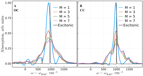
Figure 1: Absorption spectrum of model H aggregate in (A) OC and (B) CC configurations, computed with $\text{mD}_{2}$ Ansatz depth $M$. Purely excitonic spectra is also shown.

Absorption spectrum of the model H aggregate, computed with an increasing $\text{mD}_{2}$ Ansatz depth $M$, both in OC and CC arrangement, are shown in Fig. (1). In both cases, absorption spectrum converges with $M=7$ multiples, higher multiplicity spectra have been computed and are identical up to $M=11$. Absorption of the $M=1$ case, which is equivalent to using the Davydov $\text{D}_{2}$ Ansatz, has peaks in the same frequencies as the converged spectrum, however, their intensities are incorrect, some are even negative. By increasing the number of multiples considered, peak amplitudes become strictly positive. The 0-0 electronic peak can be clearly identified. Vibrational side-peaks to the higher energy side are due to 0-n vibronic transitions, while on the lower energy side reside the n-0 transition peaks, permitted by the non-zero temperature. Finite vibronic peak widths originate from the vibrational dephasing, due to finite temperature and aggregate environment fluctuations. Both the OC and CC aggregates have similar lineshapes, slightly finer vibronic structure can be observed in the CC system, due to a larger symmetry and, therefore, effectively lower broadening.

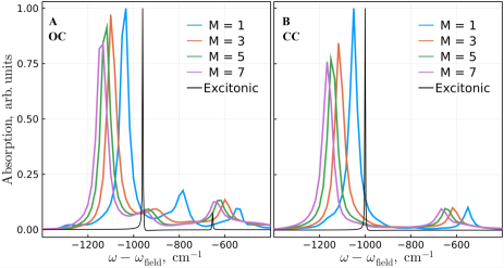
Figure 2: Absorption spectrum of model J aggregate in (A) OC and (B) CC configurations, computed with $\text{mD}_{2}$ Ansatz depth $M$. Purely excitonic spectra is also shown.

Absorption spectrum of the model J aggregate is shown in Fig. (2). In the CC aggregate, visible side-peak, on the higher energy side of the strong 0-0 transition, is the first term of vibrational progression. The effective HR factor is thus significantly reduced (hence, the exchange narrowing) due to intermolecular couplings. It is observed independent of Ansatz depth considered in both OC and CC arrangements. By increasing $M$, absorption spectrum redshifts to lower energies, while qualitatively maintaining the same shape, however, slight differences emerge. For the OC aggregate, peak intensities change, while for CC aggregate, mostly only the main peak intensity changes. Apparent energy splitting between electronic transitions is considerably reduced, implying that vibronic states do not maintain excitonic intraband gaps due to the strong intramolecular vibrational coupling. In contrast to the H aggregate, all absorption peaks are positive, even with $M=1$ multiplicity.

In order to quantify convergence of H aggregate absorption spectrum with increasing$\text{mD}_{2}$ Ansatz depth, we calculate the normalized discrepancy (Gelzinis et al., 2015)

$$\mathcal{D}\left(M\right)=\frac{1}{\mathcal{N}}\int\text{d}\omega\sqrt{\left(A\left(\omega,M\right)-\overline{A}\left(\omega\right)\right)^{2}},$$ (17)

where $A\left(\omega,M\right)$ is the absorption spectrum with multiplicity $M$, where $\overline{A}\left(\omega\right)=A\left(\omega,M=11\right)$ is the converged reference spectra and

$$\mathcal{N}=\max_{\text{over}\ M}\int\text{d}\omega\sqrt{\left(A\left(\omega,M\right)-\overline{A}\left(\omega\right)\right)^{2}},$$ (18)

is the normalization factor. In Fig. (3) we show $\mathcal{D}\left(M\right)$ for H aggregate for various values of the nearest neighbor coupling $J$, vibrational mode thermal energy $k_{\text{B}}T$, and Ansatz depth $M=1,\ldots,8$.

We observe that for CC and OC H aggregates, discrepancy significantly depends on $J$ and $k_{\text{B}}T$, even at the same depth $M$. We observe, that in the case of $M=1,$ independent of model parameters and site arrangement, spectrum discrepancy is always high. By increasing depth to just $M=2$, for some parameters, discrepancy is reduced significantly. By inspecting higher depths ($M=2-4$), a general observation can be made. Mainly, that the CC H aggregate requires larger depth at higher temperatures, while for the OC H aggregate, two parameter regions of high discrepancy can be discerned: at low temperatures, independent of the coupling strength, and at high temperatures at weak coupling. The high temperature cases can be rationalized as needing more CS to represent thermally excited QHO eigenstates with quantum numbers $n>0$, which are more probable at higher temperatures. Reasoning for the low temperature case is more subtle. Aggregate excitation via an external field shifts oscillators away from their equilibrium considerably (HR factor $S=1$), then the molecular wavepacket relaxes via vibronic state energy surfaces, which induce wavepacket shape changes and/or wavepacket splitting between vibronic surfaces. Either of these two effects would necessitate molecular aggregate wavepacket to be represented by the $\text{mD}_{2}$ Ansatz with depth $M>1$.

As seen in Fig. (2), by considering larger depth, J aggregate absorption spectrum lineshape redshifts with minimal changes to the overall shape of the spectrum, therefore, the use of discrepancy estimate in Eq. (17) is not necessary. By visually inspecting spectrum of J aggregate with various nearest neighbor couplings and temperatures (shown in Supplementary Material), we find depth of $M=7$ to again give a well converged result.

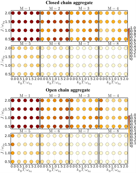
Figure 3: Normalized discrepancy $\mathcal{D}\left(M\right)$ of the H aggregate in a CC and OC configurations for a range of $J$, $k_{\text{B}}T$ values, computed with $\text{mD}_{2}$ Ansatz depth $M$.

IV Discussion

The total energy of a single QHO, represented by the $\text{D}_{2}$ Ansatz, is proportional to the CS displacement $\lambda$ from the origin, $E_{\text{D}_{2}}^{\left(\text{osc}\right)}\propto|\lambda|^{2}$, and the wavepacket shape is that of the lowest energy QHO eigenstate with quantum number $n=0$, i.e., a simple Gaussian. On the other hand, using representation of the $\text{mD}_{2}$ Ansatz, oscillator energy is proportional to the sum of products of CS displacements, $E_{\text{mD}_{2}}^{\left(\text{osc}\right)}\propto\sum_{i,j}\lambda_{i}^{\star}\lambda_{j}$, and the wavepacket now is not necessarily a Gaussian due to the interference of multiple CS. This allows $\text{mD}_{2}$ Ansatz to represent more complicated QHO eigenstate wavepackets with quantum numbers $n>0$. It should be noted, that CS can be used to represent an arbitrary wavepacket using the unity operator expression

$$\hat{I}=\pi^{-1}\iint\text{d\text{Re}$\lambda$}\ \text{d\text{Im}$\lambda$}\ |\lambda\rangle\langle\lambda|,$$ (19)

consequently, $\text{mD}_{2}$ Ansatz with infinite depth would allow for complete and exact description of a quantum system. It thus becomes important to obtain the lower limit at which the vibronic dynamics is properly described for e. g. absorption spectroscopy.

Using either of the $\text{D}_{2}$ or $\text{mD}_{2}$ representations, oscillator can have equal energy, $E_{\text{D}_{2}}^{\left(\text{osc}\right)}=E_{\text{mD}_{2}}^{\left(\text{osc}\right)}$, however, their wavepacket shape must not be equivalent. It is therefore interesting to look at vibrational mode wavepacket transition from being represented by the $\text{D}_{2}$ to a more complex $\text{mD}_{2}$ Ansatz. Such transition occurs naturally in Eq. (10), for the computation of the linear response function, when an upward transition dipole operator acts on the aggregate ground state, as given by Eq. (11). One way to track wavepacket changes, is to consider its coordinate and momentum variances, given by

$$\sigma_{x}^{2}\left(t\right) =\left\langle\hat{x}^{2}\left(t\right)\right\rangle-\left\langle\hat{x}\left(t\right)\right\rangle^{2},$$ (20)

$$\sigma_{p}^{2}\left(t\right) =\left\langle\hat{p}^{2}\left(t\right)\right\rangle-\left\langle\hat{p}\left(t\right)\right\rangle^{2},$$ (21)

where $\left\langle\mathcal{O}\left(t\right)\right\rangle=\left\langle\Psi_{\text{mD}_{2}}^{\left(\text{e}\right)}\left(t\right)\left|\hat{\mathcal{O}}\right|\Psi_{\text{mD}_{2}}^{\left(\text{e}\right)}\left(t\right)\right\rangle$ is an expectation value of operator $\hat{\mathcal{O}}$, and their average variance

$$\overline{\sigma_{x,p}^{2}}\left(t\right)=\frac{1}{2}\left(\sigma_{x}^{2}\left(t\right)+\sigma_{p}^{2}\left(t\right)\right).$$ (22)

For an independent QHO, the average variance is $\overline{\sigma_{x,p}^{2}}=n+\frac{1}{2}$, where $n$ is the QHO occupation number. In Fig. (4) we display coordinate, momentum and their average variances of vibrations coupled to the 1st and 6th sites of the J aggregate in both OC and CC configurations with depth $M=10$. In the OC configuration, 1st site is the outermost and the 6th site is in the middle of the aggregate, while in the CC, these modes are translationally invariant and represent two modes with a largest separation.

In both configurations, we observe coordinate and momentum variance oscillations in an out-of-phase manner, while at the same time, the average variance also increases, slightly more in a CC. Instead of considering superposition of CS to capture such oscillatory behavior, squeezed coherent states (SCS) could be used (Tsue and Fujiwara, 1991; Abramavičius and Marčiulionis, 2018; Chorošajev et al., 2017; Zeng and Yao, 2022), which are able to produce similar variance oscillations intrinsically . Downside of using SCS would be the need to additionally propagate variables describing squeezing amplitude and phase for each vibrational mode. In the Davydov $\text{D}_{2}$ type Ansatz with SCS, the overall increase of variance would not be captured, yet, for low temperatures, this might serve as a sufficient approximation. For high temperatures, multi-Davydov $\text{D}_{2}$ type Ansatz with SCS would be required.

In a CC configuration, due to the 10-fold symmetry of the aggregate, no difference between variance changes of vibrational modes is to be expected, while slight differences are observed due to the finite size of the thermal ensemble considered. Meanwhile, in the OC, difference between variances of the outer and inner modes can be seen. Outer vibrational mode, again, show increasing, but oscillatory dynamics, while the inner mode coordinate and momentum variance values differ, i.e., wavepacket becomes permanently more stretched along the momentum axis as compared to the coordinate axis.

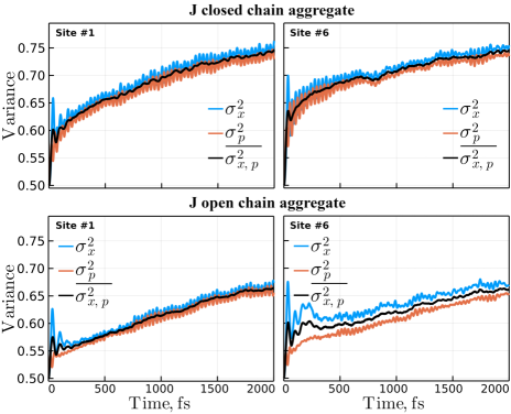
Figure 4: Coordinate, momentum and their average variances of a 1st and 6th site vibrational mode of a J aggregate in ring and chain configurations with multiplicity $M=11$.

We see, that vibrational mode variance changes without any explicit coupling term between the vibrational DOF. Previously we have proposed a simplified version of the $\text{mD}_{2}$ Ansatz, termed $\text{sD}_{2}$ (Jakučionis et al., 2020), by considering multiplicity only of vibrational mode states. We have observed that the energy transfer between vibrational modes required inclusion of quadratic or higher order Hamiltonian coupling term between oscillators, which deformed the initially quadratic oscillator potential energy surfaces. Energy transfer between vibrational modes manifested itself as an increase of vibrational mode variance. In the presented case of the $\text{mD}_{2}$ Ansatz, vibrational mode variance increase without introducing any explicit Hamiltonian coupling terms, implying that the multiplicity of the vibronic states implicitly changes the parabolic potential energy surfaces into non-parabolic. This can be understood by solving for vibronic energy surfaces the eigenstates $E(x_{1},\ldots,x_{Q})$. E.g., for a dimer aggregate, vibronic aggregate Hamiltonian $\hat{H}$ characteristic polynomial equation is equal to

$$0 =\left(\varepsilon_{1}+\omega f^{2}-x_{1}\omega f+\frac{\omega}{2}\left(x_{1}^{2}+x_{2}^{2}\right)-E(x_{1},x_{2})\right)$$

$$\times\left(\varepsilon_{2}+\omega f^{2}-x_{2}\omega f+\frac{\omega}{2}\left(x_{1}^{2}+x_{2}^{2}\right)-E(x_{1},x_{2})\right)$$

$$-J^{2},$$ (23)

solution of which, $E(x_{1},x_{2})$, is not a quadratic function of vibrational mode coordinates $x_{1}$ and $x_{2}$.

In conclusion, by inspecting absorption spectrum of a wide range of J and H molecular aggregates, in both CC and OC site configurations, with various nearest neighbor coupling strength and temperature values, we find the $\text{mD}_{2}$ Ansatz with depth of $M=7$ to be required for accurate aggregate absorption spectra simulation, while the regular Davydov $\text{D}_{2}$ Ansatz is not sufficient. For H aggregates, multiplicity is required to obtain absorption lineshape positivity and correct peak intensities. For J aggregates, increasing the number of $\text{mD}_{2}$ Ansatz depth, mostly redshifts absorption spectrum, keeping the overall lineshape qualitatively stays the same, especially in CC aggregate. However, the very exchange narrowing effect is captured by the simple Davydov $\text{D}_{2}$ Ansatz. Due to vibronic energy level structure of an aggregate, we find molecular wavefunction to exhibit an out-of-phase oscillatory behavior along the coordinate and momentum axes and an overall broadening, which again is not captured by the Davydov $\text{D}_{2}$ Ansatz.

Appendix A Multi-Davydov $\text{D}_{2}$ equations of motion and numerical implementation

Following the TDVP procedure, we derived vibronic molecular aggregate EOMs, given by

$$\sum_{j}\left(\dot{\alpha}_{j,n}S_{ij}+\alpha_{j,n}S_{ij}K_{ij}\right) =-\text{i}\Theta_{i,n},$$ (24)

for each pair of indices $\left\{i,n\right\}$, and

$$\sum_{j,n}\left(\alpha_{i,n}^{\star}\dot{\alpha}_{j,n}S_{ij}\lambda_{j,kh}+P_{ij,n}\dot{\lambda}_{j,kh}\right)$$

$$+\sum_{j,n}P_{ij,n}\lambda_{j,kh}K_{ij} =-\text{i}\Omega_{i,kh},$$ (25)

for pair of $\left\{i,k,h\right\}$ indices. These constitute a system of equations needed to solve to propagate the $\text{mD}_{2}$ Ansatz, shown in Eq. (8). Dot notation is used, where $\dot{x}$ is the time derivative of $x$. Right-hand side of given EOMs are

$$\Theta_{i,n} =\sum_{j,m}\alpha_{j,m}S_{ij}J_{nm}$$

$$+\sum_{j}\alpha_{j,n}S_{ij}\sum_{h}\left(C_{ij,nh}+\sum_{k}A_{ij,kh}\right),$$ (26)

$$\Omega_{i,kh} =\sum_{j,n,m}G_{ij,nm}\lambda_{j,kh}J_{nm}$$

$$+\sum_{j,n}P_{ij,n}\lambda_{j,kh}\sum_{q}\left(C_{ij,nq}+\sum_{f}A_{ij,fq}\right)$$

$$+\sum_{j}P_{ij,k}f_{kh}\omega_{kh}-\text{i}\sum_{j,n}P_{ij,n}\omega_{kh}\lambda_{j,kh},$$ (27)

where auxiliary definitions are

$$G_{ij,nm} =\alpha_{i,n}^{\star}\alpha_{j,m}S_{ij},$$ (28)

$$P_{ij,n} =G_{ij,nn},$$ (29)

$$A_{ij,kh} =\omega_{kh}\lambda_{i,kh}^{\star}\lambda_{j,kh},$$ (30)

$$C_{ij,nh} =-f_{nh}\omega_{nh}\left(\lambda_{i,nh}^{\star}+\lambda_{j,nh}\right),$$ (31)

$$K_{ij} =\sum_{m,h}\dot{\lambda}_{j,mh}\left(\lambda_{i,mh}^{\star}-\frac{1}{2}\lambda_{j,mh}^{\star}\right)$$ (32)

$$-\sum_{m,h}\frac{1}{2}\dot{\lambda}_{j,mh}^{\star}\lambda_{j,mh}.$$ (33)

We solved the presented system of EOMs in terms of variable $\alpha_{i,n}$, $\lambda_{i,kh}$ real and imaginary parts, which are ordered in a column state vector, $\boldsymbol{x}=\left\{\boldsymbol{\alpha}_{i,n}^{\text{R}},\boldsymbol{\alpha}_{i,n}^{\text{I}},\boldsymbol{\lambda}_{i,kh}^{\text{R}},\boldsymbol{\lambda}_{i,kh}^{\text{I}}\right\}$. This doubles the amount of variables, however, removes consistency problems regarding treatment of complex variables $\dot{\lambda}_{j,mh}$, $\dot{\lambda}_{j,mh}^{\star}$.

Numerical propagation of the $\text{mD}_{2}$ Ansatz is a two step process. First, the time derivative of a state vector, $\dot{\boldsymbol{x}}$, is found, by writing Eqs. (24), (25) in a matrix form

$$\boldsymbol{M}\dot{\boldsymbol{x}}=\boldsymbol{f},$$ (34)

and solving for $\dot{\boldsymbol{x}}$ using the Generalized Minimal Residual Method (GMRES) with Lower–Upper (LU) decomposition as a preconditioner. We found GMRES method to provide a more accurate and stable solution than using the Moore-Penrose pseudo inverse or the solely LU decomposition method. Second, the state vector now can be propagated using a variety of ordinary differential equation solvers (Rackauckas, Christopher and Nie, 2017). We found an adaptive-order adaptive-time Adams-Moulton method (VCABM) (Ernst Hairer et al., 1993) to provide just as accurate solution as a typical Runge–Kutta fourth-order method, however, with less computational effort.

During time evolution of the $\text{mD}_{2}$ Ansatz, two, or more, multiplicity wavepackets can approach each other and highly overlap, this results in an ill-conditioned coefficient matrix, $\boldsymbol{M}$, with no consistent solution of Eq. (34). To remedy this, we have implemented a programmed removal (apoptosis) of overlapping multiples of the $\text{mD}_{2}$ Ansatz, with the minimal distance for apoptosis to occur $d=0.05$, as defined in Ref. (Werther and Großmann, 2020).

Establishing scaling factor of the numerical effort required to propagate $\text{mD}_{2}$ Ansatz with increasing model size is not straightforward. The total number of complex variables, $V$, describing $\text{mD}_{2}$ Ansatz is easy to find, $V=M\cdot\left(N+K\cdot Q\right)$, however, due to first having to compute the time derivative of a state vector, $\dot{\boldsymbol{x}}$, which involves non-linear and/or iterative methods, the actual numerical effort is difficult to quantify. Empirical estimation, which would compare scaling factors of several computation approaches, is an interesting future research avenue.

References

- Davydov (1979) A. S. Davydov, Phys. Scr., 1979, 20, 387–394.
- Scott (1991) A. C. Scott, Phys. D Nonlinear Phenom., 1991, 51, 333–342.
- Sun et al. (2010) J. Sun, B. Luo and Y. Zhao, Phys. Rev. B - Condens. Matter Mater. Phys., 2010, 82, 014305.
- Chorošajev et al. (2016) V. Chorošajev, O. Rancova and D. Abramavicius, Phys. Chem. Chem. Phys., 2016, 18, 7966–7977.
- Jakučionis et al. (2018) M. Jakučionis, V. Chorošajev and D. Abramavičius, Chem. Phys., 2018, 515, 193–202.
- Jakučionis et al. (2020) M. Jakučionis, T. Mancal and D. Abramavičius, Phys. Chem. Chem. Phys., 2020, 22, 8952–8962.
- Sun et al. (2015) K. W. Sun, M. F. Gelin, V. Y. Chernyak and Y. Zhao, J. Chem. Phys., 2015, 142, 212448.
- Zhou et al. (2016) N. Zhou, L. Chen, Z. Huang, K. Sun, Y. Tanimura and Y. Zhao, J. Phys. Chem. A, 2016, 120, 1562–1576.
- Chorošajev et al. (2017) V. Chorošajev, T. Marčiulionis and D. Abramavicius, J. Chem. Phys., 2017, 147, 074114.
- Jakucionis et al. (2022) M. Jakucionis, I. Gaiziunas, J. Sulskus and D. Abramavicius, J. Phys. Chem. A, 2022, 126, 180–189.
- Glauber (1963) R. J. Glauber, Phys. Rev., 1963, 131, 2766–2788.
- Jakučionis and Abramavičius (2021) M. Jakučionis and D. Abramavičius, Phys. Rev. A, 2021, 103, 032202.
- Zhou et al. (2016) N. Zhou, L. Chen, Z. Huang, K. Sun, Y. Tanimura and Y. Zhao, J. Phys. Chem. A, 2016, 120, 1562–1576.
- Zhou et al. (2014) N. Zhou, L. Chen, D. Mozyrsky, V. Chernyak and Y. Zhao, Phys. Rev. B - Condens. Matter Mater. Phys., 2014, 90, 155135.
- Wang et al. (2016) L. Wang, L. Chen, N. Zhou and Y. Zhao, J. Chem. Phys., 2016, 144, 024101.
- Chen et al. (2019) L. Chen, M. F. Gelin and W. Domcke, J. Chem. Phys., 2019, 150, 24101.
- Gao et al. (2021) L. Gao, K. Sun, H. Zheng and Y. Zhao, Adv. Theory Simulations, 2021, 4, 2100083.
- Wang et al. (2021) L. Wang, F. Zheng, J. Wang, F. Großmann and Y. Zhao, J. Phys. Chem. B, 2021, 125, 3184–3196.
- Sun et al. (2021) K. Sun, X. Liu, W. Hu, M. Zhang, G. Long and Y. Zhao, Phys. Chem. Chem. Phys., 2021, 23, 12654–12667.
- Sun et al. (2022) K. Sun, C. Dou, M. F. Gelin and Y. Zhao, J. Chem. Phys., 2022, 156, 024102.
- Zhao et al. (2021) Y. Zhao, K. Sun, L. Chen and M. Gelin, WIREs Comput. Mol. Sci., 2021, e1589.
- McRae and Kasha (1958) E. G. McRae and M. Kasha, J. Chem. Phys., 1958, 28, 721–722.
- Kasha (1963) M. Kasha, Radiat. Res., 1963, 20, 55–70.
- Kasha et al. (1965) M. Kasha, H. R. Rawls and M. A. El-Bayoumi, Pure Appl. Chem., 1965, 11, 371–392.
- Spano (2009) F. C. Spano, Acc. Chem. Res., 2009, 43, 429–439.
- Schröter et al. (2015) M. Schröter, S. D. Ivanov, J. Schulze, S. P. Polyutov, Y. Yan, T. Pullerits and O. Kühn, Phys. Rep., 2015, 567, 1–78.
- Hestand and Spano (2018) N. J. Hestand and F. C. Spano, Chem. Rev., 2018, 118, 7069–7163.
- Eisfeld and Briggs (2006) A. Eisfeld and J. S. Briggs, Chem. Phys., 2006, 324, 376–384.
- Walczak et al. (2008) P. B. Walczak, A. Eisfeld and J. S. Briggs, J. Chem. Phys., 2008, 128, 044505.
- Roden et al. (2008) J. Roden, A. Eisfeld and J. S. Briggs, Chem. Phys., 2008, 352, 258–266.
- Valkunas et al. (2013) L. Valkunas, D. Abramavicius and T. Mančal, Molecular Excitation Dynamics and Relaxation, Wiley-VCH Verlag GmbH, 2013.
- Bardeen (2014) C. J. Bardeen, Annu. Rev. Phys. Chem., 2014, 65, 127–148.
- van Amerongen et al. (2000) H. van Amerongen, R. van Grondelle and L. Valkunas, Photosynthetic Excitons, World Scientific, 2000.
- Schröter et al. (2015) M. Schröter, S. Ivanov, J. Schulze, S. Polyutov, Y. Yan, T. Pullerits and O. Kühn, Phys. Rep., 2015, 567, 1–78.
- Mukamel (1995) S. Mukamel, Principles of nonlinear optical spectroscopy, Oxford University Press, 1995.
- Frenkel (1931) J. Frenkel, Phys. Rev., 1931, 37, 17–44.
- Bargmann et al. (1971) V. Bargmann, P. Butera, L. Girardello and J. R. Klauder, Reports Math. Phys., 1971, 2, 221–228.
- Werther and Großmann (2020) M. Werther and F. Großmann, Phys. Rev. B, 2020, 101, 174315.
- Wang et al. (2017) L. Wang, Y. Fujihashi, L. Chen and Y. Zhao, J. Chem. Phys., 2017, 146, 124127.
- Xie et al. (2017) Q. Xie, H. Zhong, M. T. Batchelor and al, J. Phys. A Math. Theor., 2017, 51, 014001.
- Gelzinis et al. (2015) A. Gelzinis, D. Abramavicius and L. Valkunas, J. Chem. Phys., 2015, 142, 154107.
- Tsue and Fujiwara (1991) Y. Tsue and Y. Fujiwara, Prog. Theor. Phys., 1991, 86, 443–467.
- Abramavičius and Marčiulionis (2018) D. Abramavičius and T. Marčiulionis, Lith. J. Phys., 2018, 58, 307–317.
- Chorošajev et al. (2017) V. Chorošajev, T. Marčiulionis and D. Abramavicius, J. Chem. Phys., 2017, 147, 074114.
- Zeng and Yao (2022) J. Zeng and Y. Yao, J. Chem. Theory Comput., 2022, acs.jctc.1c00859.
- Rackauckas, Christopher and Nie (2017) Q. Rackauckas, Christopher and Nie, J. Open Res. Softw., 2017, 5, 15.
- Ernst Hairer et al. (1993) Ernst Hairer, Gerhard Wanner and Syvert P. Nørsett, Solving Ordinary Differential Equations I, Springer Berlin Heidelberg, 1993.