R-VGAL: A Sequential Variational Bayes Algorithm for Generalised Linear Mixed Models

Abstract

Models with random effects, such as generalised linear mixed models (GLMMs), are often used for analysing clustered data. Parameter inference with these models is difficult because of the presence of cluster-specific random effects, which must be integrated out when evaluating the likelihood function. Here, we propose a sequential variational Bayes algorithm, called Recursive Variational Gaussian Approximation for Latent variable models (R-VGAL), for estimating parameters in GLMMs. The R-VGAL algorithm operates on the data sequentially, requires only a single pass through the data, and can provide parameter updates as new data are collected without the need of re-processing the previous data. At each update, the R-VGAL algorithm requires the gradient and Hessian of a “partial” log-likelihood function evaluated at the new observation, which are generally not available in closed form for GLMMs. To circumvent this issue, we propose using an importance-sampling-based approach for estimating the gradient and Hessian via Fisher’s and Louis’ identities. We find that R-VGAL can be unstable when traversing the first few data points, but that this issue can be mitigated by using a variant of variational tempering in the initial steps of the algorithm. Through illustrations on both simulated and real datasets, we show that R-VGAL provides good approximations to the exact posterior distributions, that it can be made robust through tempering, and that it is computationally efficient.

Keywords: Fisher’s identity, intractable gradient, latent variable model, Louis’ identity, variational tempering

1 Introduction

Mixed models are useful for analysing clustered data, wherein observations that come from the same cluster/group are likely to be correlated. Example datasets include records of students clustered within schools, and repeated measurements of biomarkers on patients. Mixed models account for intra-group dependencies by incorporating cluster/group-specific “random effects”. Inference with these models is made challenging by the fact that the likelihood function involves integrals over the random effects that are not usually tractable except for the few cases where the distribution of the random effects is conjugate to the distribution of the data, such as in the linear mixed model (Verbeke et al.,, 1997), the beta-binomial model (Crowder,, 1979), and Rasch’s Poisson count model (Jansen,, 1994). Notably, there is no closed-form expression for the likelihood function in the case of the ubiquitous logistic mixed model.

Maximum-likelihood-based approaches are often used for parameter inference in mixed models. In the case of linear mixed models, parameter inference via maximum likelihood estimation is straightforward (e.g., Wakefield,, 2013). For mixed models with an intractable likelihood, integrals over random effects need to be numerically approximated, for example by using Gaussian quadrature (Naylor and Smith,, 1982) or the Laplace approximation (Tierney and Kadane,, 1986). The likelihood may also be indirectly maximised using an expectation-maximisation type algorithm (Dempster et al.,, 1977), which treats the random effects as missing, and iteratively maximises the “expected complete log-likelihood” of the data and the random effects. Quasi-likelihood approaches such as penalised quasi-likelihood (PQL, Breslow and Clayton,, 1993) and marginal quasi-likelihood (MQL, Goldstein,, 1991) approximate nonlinear mixed models with linear mixed models, so that well-developed estimation routines for linear mixed models can be applied; see Tuerlinckx et al., (2006) for a detailed discussion of these methods. These maximum-likelihood-based methods provide point estimates and not full posterior distributions over the parameters.

Full posterior distributions can be obtained using Markov chain Monte Carlo (MCMC, e.g., Zhao et al.,, 2006; Fong et al.,, 2010). MCMC provides exact, sample-based posterior distributions, but at a higher computational cost than maximum-likelihood-based methods. Alternatively, variational Bayes (VB) methods (e.g., Ong et al.,, 2018; Tan and Nott,, 2018) are becoming increasingly popular for estimating parameters in complex statistical models. These methods approximate the exact posterior distribution with a member from a simple and tractable family of distributions; this family is usually chosen to balance the accuracy of the approximation against the computational cost required to obtain the approximation. VB methods are usually computationally cheaper than MCMC methods. VB approaches can either batch-process the data (e.g., Tran et al.,, 2016; Ong et al.,, 2018; Tan and Nott,, 2018) or sequentially process data points one-by-one (e.g., Broderick et al.,, 2013; Gunawan et al.,, 2021; Lambert et al.,, 2022). For settings with large amounts of data, a method that targets the posterior distribution via sequential processing of the data offers several advantages. The so-called Recursive Variational Gaussian Approximation (R-VGA, Lambert et al.,, 2022) algorithm is a recently-developed sequential variational Bayes method that provides a fast and accurate approximation to the posterior distribution with only one pass through the data, making it computationally efficient when compared to MCMC or batch variational Bayes. Lambert et al., (2022) apply the R-VGA algorithm to linear and logistic regression models without random effects.

In this paper, we build on the R-VGA algorithm by proposing a novel recursive variational Gaussian approximation, called Recursive Variational Gaussian Approximation for Latent variable models (R-VGAL), for estimating the parameters in GLMMs. At each update, R-VGAL requires the gradient and Hessian of the “partial” log-likelihood evaluated at the new observation, which are often not available in closed form. To circumvent this issue, we propose an importance-sampling-based approach for estimating the gradient and Hessian using Fisher’s and Louis’ identities  (Cappé et al.,, 2005). This approach was inspired by the work of  Nemeth et al., (2016), who used Fisher’s and Louis’ identities to approximate the gradient and Hessian in a sequential Monte Carlo context. The efficacy of R-VGAL is illustrated using linear and logistic mixed effect models on simulated and real datasets. The examples show that R-VGAL provides good approximations to the exact posterior distributions estimated using Hamiltonian Monte Carlo (HMC, Neal,, 2011; Betancourt and Girolami,, 2015) and at a low computational cost.

The paper is organised as follows. Section 2 presents the R-VGAL algorithm. Section 3 applies the R-VGAL algorithm to simulated and real datasets. Section 4 concludes with a discussion of our results and an overview of future research directions. This article has an online supplement containing additional technical details, and the code to reproduce results from the simulation and real-data experiments is available on https://github.com/bao-anh-vu/R-VGAL.

2 The R-VGAL Algorithm

This section reviews GLMMs (Breslow and Clayton,, 1993), and then introduces the R-VGAL algorithm for making parameter inference with these models.

2.1 Generalised linear mixed models

GLMMs are statistical models that contain both fixed effects and random effects. Typically, the fixed effects are common across groups, while the random effects are group-specific, and this is the setting we focus on.

Denote by $y_{ij}$ the $j$th response in the $i$th group, for $i=1,\dots,N$ groups and $j=1,\dots,n_{i}$, where $n_{i}$ is the number of responses in group $i$. Let $\mathbf{y}\equiv({\mathbf{y}_{1}^{\top},\dots,\mathbf{y}_{N}^{\top}})^{\top}$ be a vector of observations, where $\mathbf{y}_{i}\equiv(y_{i1},\dots,y_{in_{i}})^{\top}$ are the responses from the $i$th group. The GLMMs we consider are constructed by first assigning each $y_{ij}$ a distribution $y_{ij}\mid\bm{\beta},\bm{\alpha}_{i},\phi\sim p(\cdot)$, where $p(\cdot)$ is a member of the exponential family with a dispersion parameter $\phi$ that is usually related to the variance of the datum, $\bm{\beta}$ are the fixed effect parameters, and $\bm{\alpha}_{i}$ are the group-specific random effects for $i=1,\dots,N$. Then, the mean of the responses, $\mu_{ij}=\mathbb{E}(y_{ij}\mid\bm{\beta},\bm{\alpha}_{i},\phi)$, is modelled as

$$g(\mu_{ij})=\mathbf{x}_{ij}^{\top}\bm{\beta}+\mathbf{z}_{ij}^{\top}\bm{\alpha}_{i},\quad i=1,\dots,N,\quad j=1,\dots,n_{i},$$ (1)

where $\mathbf{x}_{ij}$ is a vector of fixed effect covariates corresponding to the $j$th response in the $i$th group; $\mathbf{z}_{ij}$ is a vector of predictor variables corresponding to the $j$th response and the $i$th random effect; and $g(\cdot)$ is a link function that links the response mean $\mu_{ij}$ to the linear predictor $\mathbf{x}_{ij}^{\top}\bm{\beta}+\mathbf{z}_{ij}^{\top}\bm{\alpha}_{i}$. We further assume that $\bm{\alpha}_{i}\perp\!\!\!\!\perp\bm{\alpha}_{j}$ for $i\neq j$. The random effects $\bm{\alpha}_{i}$, for $i=1,\dots,N$, are assumed to follow a normal distribution with mean $\mathbf{0}$ and covariance matrix $\mathbf{\Sigma}_{\alpha}$, that is, each $\bm{\alpha}_{i}\mid\mathbf{\Sigma}_{\alpha}\sim N(\mathbf{0},\mathbf{\Sigma}_{\alpha})$. In practice, some structure is often assumed for the random effects covariance matrix so that it is parameterised in terms of a smaller number of parameters $\bm{\tau}$, that is, $\mathbf{\Sigma}_{\alpha}=\mathbf{\Sigma}_{\alpha}(\bm{\tau})$. Inference is then made on the parameters $\bm{\theta}=(\bm{\beta}^{\top},\bm{\tau}^{\top},\phi)^{\top}$.

The main objective of Bayesian inference is to obtain the posterior distribution of the model parameters $\bm{\theta}$ given the observations $\mathbf{y}$ and the prior distribution $p(\bm{\theta})$. Through Bayes rule, the posterior distribution of $\bm{\theta}$ is

$$p(\bm{\theta}\mid\mathbf{y})=p(\bm{\beta},\bm{\tau},\phi\mid\mathbf{y})\propto p(\mathbf{y}\mid\bm{\beta},\bm{\tau},\phi)p(\bm{\beta},\bm{\tau},\phi).$$ (2)

The likelihood function,

$$p(\mathbf{y}\mid\bm{\beta},\bm{\tau},\phi)=\prod_{i=1}^{N}\int p(\mathbf{y}_{i}\mid\bm{\alpha}_{i},\bm{\beta},\phi)p(\bm{\alpha}_{i}\mid\bm{\tau})\,\mathrm{d}\bm{\alpha}_{i},$$ (3)

involves integrals over the random effects $\bm{\alpha}_{i},i=1,\dots,N$. The likelihood function can be calculated exactly for the linear mixed model with normally distributed random effects, for which

$$y_{ij}=\mathbf{x}_{ij}^{\top}\bm{\beta}+\mathbf{z}_{ij}^{\top}\bm{\alpha}_{i}+\epsilon_{ij},\quad\bm{\alpha}_{i}\sim N(\mathbf{0},\mathbf{\Sigma}_{\alpha}(\bm{\tau})),\quad\epsilon_{ij}\sim N(0,\sigma_{\epsilon}^{2}),$$ (4)

for $i=1,\dots,N$ and $j=1,\dots,n_{i}$, where $\epsilon_{ij}$ is a zero-mean, normally distributed error term with variance $\sigma_{e}^{2}$ that is associated with the $j$th response from the $i$th group. At the group level, this model can be written as

$$\mathbf{y}_{i}=\mathbf{X}_{i}\bm{\beta}+\mathbf{Z}_{i}\bm{\alpha}_{i}+\bm{\varepsilon}_{i},\quad\bm{\alpha}_{i}\sim N(\mathbf{0},\mathbf{\Sigma}_{\alpha}(\bm{\tau})),\quad\bm{\varepsilon}_{i}\sim N(\sigma_{\epsilon}^{2}\mathbf{I}_{n_{i}})$$

where $\mathbf{X}_{i}=(\mathbf{x}_{i1},\dots,\mathbf{x}_{in_{i}})^{\top}$, and $\mathbf{Z}_{i}=(\mathbf{z}_{i1},\dots,\mathbf{z}_{in_{i}})^{\top}$, with $n_{i}$ being the number of observations in the $i$th group, for $i=1,\dots,N$. The likelihood function for this linear mixed model is

$$p(\mathbf{y}\mid\bm{\beta},\bm{\tau},\sigma_{\epsilon}^{2})=\prod_{i=1}^{N}p(\mathbf{y}_{i}\mid\bm{\beta},\bm{\tau},\sigma_{\epsilon}^{2})=\prod_{i=1}^{N}N(\mathbf{X}_{i}\bm{\beta},\mathbf{Z}_{i}\mathbf{\Sigma}_{\alpha}(\tau)\mathbf{Z}_{i}^{\top}+\sigma_{\epsilon}^{2}\mathbf{I}_{n_{i}}).$$ (5)

The gradient and Hessian of the log-likelihood for the linear mixed model are also available in closed form. However, the likelihood $p(\mathbf{y}_{i}\mid\bm{\alpha}_{i},\bm{\beta},\phi)$ in (3) cannot be computed exactly for general random effects models. One important case is the logistic mixed model given by

$$y_{ij}\sim\text{Bernoulli}(\pi_{ij}),\quad\text{logit}(\pi_{ij})=\mathbf{x}_{ij}^{\top}\bm{\beta}+\mathbf{z}_{ij}^{\top}\bm{\alpha}_{i},\quad i=1,\dots,N,\quad j=1,\dots,n_{i},$$ (6)

where $\text{logit}(\pi_{ij})=\log\left(\frac{\pi_{ij}}{1-\pi_{ij}}\right)$. The likelihood function for this model can, however, be estimated unbiasedly, as we show in Section 2.3.

2.2 The R-VGAL algorithm

VB is usually used for posterior inference in complex statistical models when inference using asymptotically exact methods such as MCMC is too costly; for a review see, for example, Blei et al., (2017). Let $\bm{\theta}$ be a vector of model parameters. Here, we consider the class of VB methods where the posterior distribution $p(\bm{\theta}\mid\mathbf{y})$ is approximated by a tractable density $q(\bm{\theta};\bm{\lambda})$ parameterised by $\bm{\lambda}$. The variational parameters $\bm{\lambda}$ are optimised by minimising the Kullback-Leibler (KL) divergence between the variational distribution and the posterior distribution, that is, by minimising

$$\text{KL}(q(\bm{\theta};\bm{\lambda})\;\|\;p(\bm{\theta}\mid\mathbf{y}))\equiv\int q(\bm{\theta};\bm{\lambda})\log\frac{q(\bm{\theta};\bm{\lambda})}{p(\bm{\theta}\mid\mathbf{y})}\,\mathrm{d}\bm{\theta}.$$ (7)

Many VB algorithms require processing the data as a batch; see, for example,  Ong et al., (2018) and Tan and Nott, (2018). The variational parameters $\bm{\lambda}$ are typically updated iteratively using stochastic gradient descent (Hoffman et al.,, 2013; Kingma and Welling,, 2013). In settings with large amounts of data or continuously-arriving data, it is often more practical to use online or sequential variational Bayes algorithms that update the approximation to the posterior distribution sequentially as new observations become available. These online/sequential algorithms are designed to handle data that are too large to fit in memory or that arrive in a continuous stream.

In a sequential VB framework, such as that proposed by Broderick et al., (2013), the observations $\mathbf{y}_{1},\dots,\mathbf{y}_{N}$ are incorporated one by one so that at iteration $i$, $i=1,\dots,N$, one targets an approximation $q_{i}(\bm{\theta})\equiv q(\bm{\theta};\bm{\lambda}_{i})$ that is closest in a KL sense to $p(\bm{\theta}\mid\mathbf{y}_{1:i})$, the posterior distribution of the parameters given data up to the $i$th observation. In this framework, $q_{i-1}(\bm{\theta})$ is treated as the “prior” for the next iteration $i$, and the KL divergence between $q_{i}(\bm{\theta})$ and the “pseudo-posterior” $p(\mathbf{y}_{i}\mid\bm{\theta})q_{i-1}(\bm{\theta})/\mathcal{Z}_{i}$, where

$$\mathcal{Z}_{i}=\int p(\mathbf{y}_{i}\mid\bm{\theta})q_{i-1}(\bm{\theta})\,\mathrm{d}\bm{\theta},$$ (8)

is minimised at each iteration. To approximate the posterior $p(\bm{\theta}\mid\mathbf{y}_{1:i})$, Broderick et al., (2013) use a mean field VB approach (e.g., Ormerod and Wand,, 2010), which assumes no posterior dependence between the elements of $\bm{\theta}$. The R-VGA algorithm proposed by Lambert et al., (2022) follows closely that of Broderick et al., (2013), but uses a variational distribution of the form $q_{i}(\bm{\theta})=N(\bm{\mu}_{i},\mathbf{P}_{i})$, where $\mathbf{P}_{i}$ is a full covariance matrix, and seeks closed-form updates for $\bm{\lambda}_{i}\equiv\{\bm{\mu}_{i},\mathbf{P}_{i}\}$ that minimise the KL divergence between $q_{i}(\bm{\theta})$ and ${p(\mathbf{y}_{i}\mid\bm{\theta})q_{i-1}(\bm{\theta})/\mathcal{Z}_{i}}$ for $i=1,\dots,N$.

Another sequential VB algorithm that is similar to that of Broderick et al., (2013) is the Updating Variational Bayes (UVB, Tomasetti et al.,, 2022) algorithm, which uses stochastic gradient descent (SGD, Bottou,, 2010) at every iteration, $i=1,\dots,N$, to minimise the KL divergence between $q_{i}(\bm{\theta})$ and ${p(\mathbf{y}_{i}\mid\bm{\theta})q_{i-1}(\bm{\theta})/\mathcal{Z}_{i}}$. One advantage of R-VGA compared to UVB is that it does not require running a full optimisation algorithm at each iteration, since updates for $\bm{\lambda}_{i}$ are available in closed form.

The R-VGA algorithm requires the gradient $\nabla_{\theta}\log p(\mathbf{y}_{i}\mid\bm{\theta})$ and Hessian $\nabla_{\theta}^{2}\log p(\mathbf{y}_{i}\mid\bm{\theta})$ of the “partial” log-likelihood for the $i$th observation. However, for the GLMMs discussed in Section 2.1, there are usually no closed-form expressions for said quantities. Our R-VGAL algorithm circumvents this issue by replacing $\nabla_{\theta}\log p(\mathbf{y}_{i}\mid\bm{\theta})$ and $\nabla^{2}_{\theta}\log p(\mathbf{y}_{i}\mid\bm{\theta})$ with their unbiased estimates, $\hstretch{4}{\widehat{\hstretch{.25}{\nabla_{\theta}\log p(\mathbf{y}_{i}\mid\bm{\theta})}}}$ and $\hstretch{4}{\widehat{\hstretch{.25}{\nabla^{2}_{\theta}\log p(\mathbf{y}_{i}\mid\bm{\theta})}}}$, respectively. These unbiased estimates are obtained by using an importance-sampling-based approach applied to Fisher’s and Louis’ identities (Cappé et al.,, 2005), which we discuss in more detail in Section 2.3. We summarise the R-VGAL algorithm in Algorithm 1.

To approximate the expectations with respect to $q_{i-1}(\bm{\theta})$ in the updates of the variational mean and precision matrix in Algorithm 1, we generate Monte Carlo samples, ${\bm{\theta}^{(l)}\sim q_{i-1}(\bm{\theta})}$, $l=1,\dots,S$, and compute:

$$\mathbb{E}_{q_{i-1}}(\nabla_{\theta}\log p(\mathbf{y}_{i}\mid\bm{\theta})) \approx\frac{1}{S}\sum_{l=1}^{S}\hstretch{4}{\widehat{\hstretch{.25}{\nabla_{\theta}\log p(\mathbf{y}_{i}\mid\bm{\theta}^{(l)})}}}$$

$$\mathbb{E}_{q_{i-1}}(\nabla_{\theta}^{2}\log p(\mathbf{y}_{i}\mid\bm{\theta})) \approx\frac{1}{S}\sum_{l=1}^{S}\hstretch{4}{\widehat{\hstretch{.25}{\nabla_{\theta}^{2}\log p(\mathbf{y}_{i}\mid\bm{\theta}^{(l)})}}},$$

for $i=1,\dots,N$.

Algorithm 1 R-VGAL

Input: observations $\mathbf{y}_{1},\dots,\mathbf{y}_{N}$, initial values $\bm{\mu}_{0}$ and $\mathbf{P}_{0}$.

Output: variational parameters $\bm{\mu}_{i}$ and $\mathbf{P}_{i}$, for $i=1,...,N$.

Set $q_{0}(\bm{\theta})=N(\bm{\mu}_{0},\mathbf{P}_{0})$

for $i=1,\dots,N$ do

     $\bm{\mu}_{i}=\bm{\mu}_{i-1}+\mathbf{P}_{i}\mathbb{E}_{q_{i-1}}(\hstretch{4}{\widehat{\hstretch{.25}{\nabla_{\theta}\log p(\mathbf{y}_{i}\mid\bm{\theta})}}})$

     $\mathbf{P}_{i}^{-1}=\mathbf{P}_{i-1}^{-1}-\mathbb{E}_{q_{i-1}}(\hstretch{4}{\widehat{\hstretch{.25}{\nabla_{\theta}^{2}\log p(\mathbf{y}_{i}\mid\bm{\theta})}}})$

end for

2.3 Approximations of the likelihood gradient and Hessian

This section discusses approaches to obtain unbiased estimates of the gradient and the Hessian of the log-likelihood with respect to the parameters.

2.3.1 Approximation of the gradient with Fisher’s identity

Consider the $i$th iteration. Fisher’s identity (Cappé et al.,, 2005) for the gradient of $\log p(\mathbf{y}_{i}\mid\bm{\theta})$ is

$$\nabla_{\theta}\log p(\mathbf{y}_{i}\mid\bm{\theta})=\int\nabla_{\theta}\log p(\mathbf{y}_{i},\bm{\alpha}_{i}\mid\bm{\theta})p(\bm{\alpha}_{i}\mid\mathbf{y}_{i},\bm{\theta})\,\mathrm{d}\bm{\alpha}_{i}.$$ (9)

If it is possible to sample directly from $p(\bm{\alpha}_{i}\mid\mathbf{y}_{i},\bm{\theta})$ (e.g., as it is with the linear random effects model in Section 3.1), the above identity can be approximated by

$$\nabla_{\theta}\log p(\mathbf{y}_{i}\mid\bm{\theta})\approx\frac{1}{S_{\alpha}}\sum_{s=1}^{S_{\alpha}}\nabla_{\theta}\log p(\mathbf{y}_{i},\bm{\alpha}_{i}^{(s)}\mid\bm{\theta}),\quad\bm{\alpha}_{i}^{(s)}\sim p(\bm{\alpha}_{i}\mid\mathbf{y}_{i},\bm{\theta}).$$ (10)

In the case where direct sampling from $p(\bm{\alpha}_{i}\mid\mathbf{y}_{i},\bm{\theta})$ is difficult, we use importance sampling (e.g., Gelman et al.,, 2004) to estimate the gradient of the log-likelihood in (9). Specifically, we draw samples ${\{\bm{\alpha}_{i}^{(s)}:s=1,\dots,S_{\alpha}\}}$ from an importance distribution $r(\bm{\alpha}_{i}\mid\mathbf{y}_{i},\bm{\theta})$, and then compute the weights

$$w^{(s)}_{i}=\frac{p(\mathbf{y}_{i}\mid\bm{\alpha}_{i}^{(s)},\bm{\theta})p(\bm{\alpha}_{i}^{(s)}\mid\bm{\theta})}{r(\bm{\alpha}_{i}^{(s)}\mid\mathbf{y}_{i},\bm{\theta})},\quad s=1,\dots,S_{\alpha}.$$

The gradient of the log-likelihood is then approximated as

$$\nabla_{\theta}\log p(\mathbf{y}_{i}\mid\bm{\theta})\approx\sum_{s=1}^{S_{\alpha}}\bar{w}_{i}^{(s)}\nabla_{\theta}\log p(\mathbf{y}_{i},\bm{\alpha}_{i}^{(s)}\mid\bm{\theta}),$$ (11)

where $\mathcal{W}_{i}\equiv\{\bar{w}^{(s)}_{i}:s=1,\dots,S_{\alpha}\}$ are the normalised weights given by

$$\bar{w}^{(s)}_{i}=\frac{w^{(s)}_{i}}{\sum_{q=1}^{S_{\alpha}}w^{(q)}_{i}},\quad s=1,\dots,S_{\alpha}.$$

One possible choice for the importance distribution is the distribution of the random effects, that is, $p(\bm{\alpha}_{i}\mid\bm{\theta})$. In this case, the weights $\mathcal{W}_{i}$ reduce to

$$w^{(s)}_{i}=p(\mathbf{y}_{i}\mid\bm{\alpha}_{i}^{(s)},\bm{\theta}),\quad s=1,\dots,S_{\alpha}.$$

We use this importance distribution in all of the illustrations in Section 3.

2.3.2 Approximation of the Hessian with Louis’ identity

Consider again the $i$th iteration. Louis’ identity (Cappé et al.,, 2005) for the Hessian $\nabla^{2}_{\theta}\log p(\mathbf{y}_{i}\mid\bm{\theta})$ is

$$-\nabla^{2}_{\theta}\log p(\mathbf{y}_{i}\mid\bm{\theta})=\nabla_{\theta}\log p(\mathbf{y}_{i}\mid\bm{\theta})\nabla_{\theta}\log p(\mathbf{y}_{i}\mid\bm{\theta})^{\top}-\frac{\nabla^{2}_{\theta}p(\mathbf{y}_{i}\mid\bm{\theta})}{p(\mathbf{y}_{i}\mid\bm{\theta})},$$ (12)

where

$$\frac{\nabla^{2}_{\theta}p(\mathbf{y}_{i}\mid\bm{\theta})}{p(\mathbf{y}_{i}\mid\bm{\theta})}= \int\nabla_{\theta}\log p(\mathbf{y}_{i},\bm{\alpha}_{i}\mid\bm{\theta})\nabla_{\theta}\log p(\mathbf{y}_{i},\bm{\alpha}_{i}\mid\bm{\theta})^{\top}p(\bm{\alpha}_{i}\mid\mathbf{y}_{i},\bm{\theta})\,\mathrm{d}\bm{\alpha}_{i}$$

$$+\int\nabla^{2}_{\theta}\log p(\mathbf{y}_{i},\bm{\alpha}_{i}\mid\bm{\theta})p(\bm{\alpha}_{i}\mid\mathbf{y}_{i},\bm{\theta})\,\mathrm{d}\bm{\alpha}_{i}.$$ (13)

The first term on the right-hand side of (12) is obtained using Fisher’s identity, as discussed in Section 2.3.1. The second term consists of two integrals (see (13)), which can also be approximated using samples. Specifically,

$$\frac{\nabla^{2}_{\theta}p(\mathbf{y}_{i}\mid\bm{\theta})}{p(\mathbf{y}_{i}\mid\bm{\theta})}\approx \frac{1}{S_{\alpha}}\sum_{s=1}^{S_{\alpha}}\left(\nabla_{\theta}\log p(\mathbf{y}_{i},\bm{\alpha}_{i}^{(s)}\mid\bm{\theta})\nabla_{\theta}\log p(\mathbf{y}_{i},\bm{\alpha}_{i}^{(s)}\mid\bm{\theta})^{\top}+\nabla^{2}_{\theta}\log p(\mathbf{y}_{i},\bm{\alpha}_{i}^{(s)}\mid\bm{\theta})\right),$$

where $\bm{\alpha}_{i}^{(s)}\sim p(\bm{\alpha}_{i}\mid\mathbf{y}_{i},\bm{\theta})$ for $s=1,\dots,S_{\alpha}$. If obtaining samples from $p(\bm{\alpha}_{i}\mid\mathbf{y}_{i},\bm{\theta})$ is not straightforward, importance sampling (as in Section 2.3.1) can be used instead. In this case, for computational efficiency, the same samples $\{\bm{\alpha}_{i}^{(s)}:s=1,\dots,S_{\alpha}\}$ that were used to approximate the score using Fisher’s identity, along with their corresponding normalised weights $\mathcal{W}_{i}$, can also be used to obtain the estimates of the second term in Louis’ identity. Then

$$\frac{\nabla^{2}_{\theta}p(\mathbf{y}_{i}\mid\bm{\theta})}{p(\mathbf{y}_{i}\mid\bm{\theta})}\approx\sum_{s=1}^{S_{\alpha}}\bar{w}^{(s)}_{i}\left(\nabla_{\theta}\log p(\mathbf{y}_{i},\bm{\alpha}_{i}^{(s)}\mid\bm{\theta})\nabla_{\theta}\log p(\mathbf{y}_{i},\bm{\alpha}_{i}^{(s)}\mid\bm{\theta})^{\top}+\nabla^{2}_{\theta}\log p(\mathbf{y}_{i},\bm{\alpha}_{i}^{(s)}\mid\bm{\theta})\right).$$

2.4 Variational tempering

A possible problem with R-VGAL is its instability during the first few iterations. Figures S13 and S14 in Section S3 of the online supplement show that the first few observations can heavily influence the trajectory of the variational mean, making the R-VGAL parameter estimates sensitive to the ordering of the observations. Here, we propose a tempering approach to stabilise the R-VGAL algorithm during the initial few steps.

In standard batch variational tempering (e.g., Mandt et al.,, 2016; Huang et al.,, 2018), tempering is used to smooth out the objective function by “down weighting” the likelihood $p(\mathbf{y}\mid\bm{\theta})$ with a tempering sequence $0<a_{1}<\dots<a_{M}=1$, thereby preventing the optimisation from getting stuck in local optima. Tempering is done by optimising the KL divergence between the variational objective $q(\bm{\theta};\bm{\lambda})$ and a sequence of “tempered” distributions given by $\eta_{m}(\cdot)=p(\mathbf{y}\mid\bm{\theta})^{a_{m}}p(\bm{\theta})/\mathcal{Z}_{m}$, where

$$\mathcal{Z}_{m}=\int p(\mathbf{y}\mid\bm{\theta})^{\alpha_{m}}p(\bm{\theta})\,\mathrm{d}\bm{\theta},$$

for $m=1,\dots,M$. The original objective function is recovered when $a_{m}=1$.

We propose a version of R-VGAL with tempering as shown in Algorithm 2. In this version, the R-VGAL updates of the mean and precision matrix for each observation are split into $K$ steps. In each step, we multiply the gradient and the Hessian of $\log p(\mathbf{y}_{i}\mid\bm{\theta})$ by a factor $a=\frac{1}{K}$ (which acts as a “step size”), and then update the variational parameters $K$ times during the $i$th iteration. Using a smaller step size helps stabilise the R-VGAL algorithm, particularly during the first few observations. Section S3 of the online supplement shows that adding tempering for the first few observations makes the R-VGAL algorithm more robust to different orderings of the data.

Algorithm 2 R-VGAL with tempering

Input: observations $\mathbf{y}_{1},\dots,\mathbf{y}_{N}$, initial values $\bm{\mu}_{0}$ and $\mathbf{P}_{0}$, number of observations to temper $n_{temp}$, number of tempering steps $K$

Output: variational parameters $\bm{\mu}_{i}$ and $\mathbf{P}_{i}$, for $i=1,...,N$.

Set $q_{0}(\bm{\theta})=N(\bm{\mu}_{0},\mathbf{P}_{0})$

for $i=1,\dots,N$ do

     if $i\leq n_{temp}$ then

         Set $a=1/K$, $\bm{\mu}_{i,0}=\bm{\mu}_{i-1},\mathbf{P}_{i,0}=\mathbf{P}_{i-1}$

         for $k=1,\dots,K$ do

              Set $q_{i,k-1}(\bm{\theta})=N(\bm{\mu}_{i,k-1},\mathbf{P}_{i,k-1})$

              $\bm{\mu}_{i,k}=\bm{\mu}_{i,k-1}+a\mathbf{P}_{i,k}\mathbb{E}_{q_{i,k-1}}(\hstretch{4}{\widehat{\hstretch{.25}{{\nabla_{\theta}\log p(\mathbf{y}_{i}\mid\bm{\theta})}}}})$

              $\mathbf{P}_{i,k}^{-1}=\mathbf{P}_{i,k-1}^{-1}-a\mathbb{E}_{q_{i,k-1}}(\hstretch{4}{\widehat{\hstretch{.25}{\nabla_{\theta}^{2}\log p(\mathbf{y}_{i}\mid\bm{\theta})}}})$

         end for

         Set $\bm{\mu}_{i}=\bm{\mu}_{i,K},\mathbf{P}_{i}=\mathbf{P}_{i,K}$, $q_{i}(\bm{\theta})=N(\bm{\mu}_{i},\mathbf{P}_{i})$

     else

         $\bm{\mu}_{i}=\bm{\mu}_{i-1}+\mathbf{P}_{i}\mathbb{E}_{q_{i-1}}(\hstretch{4}{\widehat{\hstretch{.25}{\nabla_{\theta}\log p(\mathbf{y}_{i}\mid\bm{\theta})}}})$

         $\mathbf{P}_{i}^{-1}=\mathbf{P}_{i-1}^{-1}-\mathbb{E}_{q_{i-1}}(\hstretch{4}{\widehat{\hstretch{.25}{\nabla_{\theta}^{2}\log p(\mathbf{y}_{i}\mid\bm{\theta})}}})$

     end if

end for

3 Applications of R-VGAL

In this section, we apply R-VGAL to estimate parameters in linear and logistic mixed models using two simulated datasets and two real datasets: the Six City dataset from Fitzmaurice and Laird, (1993), and the POLYPHARMACY dataset from Hosmer et al., (2013). We validate R-VGAL against Hamiltonian Monte Carlo (HMC, Neal,, 2011; Betancourt and Girolami,, 2015), which we implement using the Stan programming language (Stan Development Team,, 2023) in R software (R Core Team,, 2022). For all examples, we run HMC for $15000$ iterations and discard the first $5000$ as burn in. Reproducible code for all examples is available on https://github.com/bao-anh-vu/R-VGAL.

3.1 Linear mixed effect model

In this example, we generate data from a linear mixed model with $N=200$ groups and $n=10$ responses per group. The $j$th response from the $i$th group is modelled as

$$y_{ij}=\mathbf{x}_{ij}^{\top}\bm{\beta}+z_{ij}\alpha_{i}+\epsilon_{ij},\quad\alpha_{i}\sim N(0,\sigma_{\alpha}^{2}),\quad\epsilon_{ij}\sim N(0,\sigma_{\epsilon}^{2}),$$ (14)

for $i=1,\dots,N$ and $j=1,\dots,n$, where $\mathbf{x}_{ij}$ is drawn from a $N(\mathbf{0},\mathbf{I}_{4})$ distribution and $z_{ij}$ is drawn from a $N(0,1)$ distribution. The true parameter values are $\bm{\beta}=(-1.5,1.5,0.5,0.25)^{\top}$, $\sigma_{\alpha}=0.9$, and $\sigma_{\epsilon}=0.7$. Since R-VGAL uses a multivariate normal distribution as the variational approximation, we consider the log-transformed variables $\phi_{\alpha}=\log(\sigma_{\alpha}^{2})$ and $\phi_{\epsilon}=\log(\sigma_{\epsilon}^{2})$ so that $\phi_{\alpha}$ and $\phi_{\epsilon}$ are unconstrained. We then make inference on the parameters $\bm{\theta}=(\bm{\beta}^{\top},\phi_{\alpha},\phi_{\epsilon})^{\top}$ using R-VGAL.

At the group level, the linear mixed model is

$$\mathbf{y}_{i}=\mathbf{X}_{i}\bm{\beta}+\mathbf{z}_{i}\alpha_{i}+\bm{\varepsilon}_{i},\quad i=1,\dots,N,$$ (15)

where $\mathbf{y}_{i}=(y_{i1},\dots,y_{in})^{\top}$, $\mathbf{X}_{i}=(\mathbf{x}_{i1},\dots,\mathbf{x}_{in})^{\top},\mathbf{z}_{i}=(z_{i1},\dots,z_{in})^{\top}$, and $\bm{\varepsilon}_{i}=(\epsilon_{i1},\dots,\epsilon_{in})^{\top}$. At each iteration, $i=1,\dots,N$, the R-VGAL algorithm makes use of the “partial” likelihood of the observations from the $i$th group, $p(\mathbf{y}_{i}\mid\bm{\theta})=N(\bm{\mu}_{y\mid\theta},\mathbf{\Sigma}_{y\mid\theta})$, where $\bm{\mu}_{y\mid\theta}=\mathbf{X}_{i}\bm{\beta}$ and $\mathbf{\Sigma}_{y\mid\theta}=\sigma_{\alpha}^{2}\mathbf{z}_{i}\mathbf{z}_{i}^{\top}+\sigma_{\epsilon}^{2}\mathbf{I}_{n}$. For this model, the gradient and Hessian of $\log p(\mathbf{y}_{i}\mid\bm{\theta})$ with respect to each of the parameters are available in closed form; see Section S1.1 of the online supplement. In this case, we are therefore able to compare the accuracy of R-VGAL implemented using approximate gradients and Hessians with that of R-VGAL implemented using exact gradients and Hessians.

The prior distribution we use, which is also the “initial” variational distribution, is

$$p(\bm{\theta})=q_{0}(\bm{\theta})=N\left(\begin{bmatrix}\mathbf{0}\\ \log(0.5^{2})\\ \log(0.5^{2})\end{bmatrix},\begin{bmatrix}10\mathbf{I}_{4}&\mathbf{0}&\mathbf{0}\\ \mathbf{0}&1&0\\ \mathbf{0}&0&1\\ \end{bmatrix}\right).$$ (16)

A $N(\log(0.5^{2}),1)$ prior distribution for $\phi_{\alpha}$ and $\phi_{\epsilon}$ is equivalent to a log-normal prior distribution with mean 0.41 and variance 0.29 for both $\sigma_{\alpha}^{2}$ and $\sigma_{\epsilon}^{2}$. Using this prior distribution, the $2.5$th and $97.5$th percentiles for both $\sigma_{\alpha}^{2}$ and $\sigma_{\epsilon}^{2}$ are $(0.035,1.775)$.

We run R-VGAL with variational tempering as described in Section 2.4 with $n_{temp}=10$ tempered observations and $K=4$ tempering steps per observation. At each iteration $i=1,\dots,200$, when approximating the gradient and Hessian of $\log p(\mathbf{y}_{i}\mid\bm{\theta})$ using Fisher’s and Louis’ identities, we use $S_{\alpha}=100$ Monte Carlo samples (of $\alpha_{i}$). When approximating the expectations with respect to $q_{i-1}(\bm{\theta})$ in the R-VGAL updates of the mean and precision matrix, we use $S=100$ Monte Carlo samples (of $\bm{\theta}$). This value of $S$ was chosen based on an experimental study on the effect of $S$ and $S_{\alpha}$ on the posterior estimates of R-VGAL in Section S2 of the online supplement.

We validate R-VGAL against HMC (Neal,, 2011; Betancourt and Girolami,, 2015), which we implemented in Stan. Figure 1 shows the marginal posterior distributions of the parameters, along with bivariate posterior distributions as estimated using R-VGAL with approximate gradients and Hessians, R-VGAL with exact gradients and Hessians, and HMC. The posterior distributions obtained using R-VGAL are clearly very similar to those obtained using HMC, irrespective of whether exact or approximate gradients and Hessians are used.

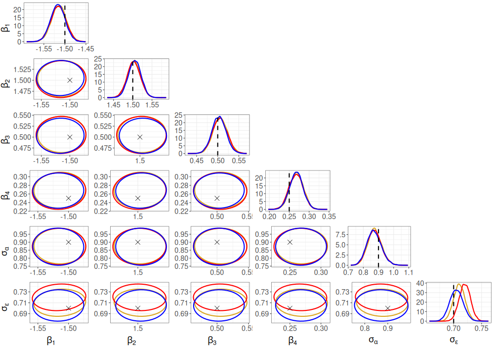
Figure 1: Exact posterior distributions (from HMC, in blue) and approximate posterior distributions (from R-VGAL with estimated gradients and Hessians in red, and from R-VGAL with exact gradients and Hessians in yellow) for the linear mixed model experiment. Diagonal panels: Marginal posterior distributions with true parameters denoted using dotted lines. Off-diagonal panels: Bivariate posterior distributions with true parameters denoted using the symbol $\times$.

3.2 Logistic mixed effect model

In this example, we generate simulated data from a random effect logistic regression model with $N=500$ groups and $n=10$ responses per group. The random effect logistic regression model we use is

$$y_{ij}\sim\textrm{Bernoulli}(\pi_{ij}),\quad\pi_{ij}=p(y_{ij}=1\mid\bm{\beta},\tau^{2})=\frac{\exp(\mathbf{x}_{ij}^{\top}\bm{\beta}+\alpha_{i})}{1+\exp(\mathbf{x}_{ij}^{\top}\bm{\beta}+\alpha_{i})},\quad\alpha_{i}\sim N(0,\tau^{2}),$$ (17)

where $\mathbf{x}_{ij}$ is drawn from a $N(\mathbf{0},\mathbf{I}_{4})$ distribution, and $z_{ij}$ is drawn from a $N(0,1)$ distribution, for $i=1,\dots,N$ and $j=1,\dots,n$. The true parameter values are $\bm{\beta}=(-1.5,1.5,0.5,0.25)^{\top}$ and $\tau=0.9$.

As in the linear case, although the parameters of the model are $\bm{\beta}$ and $\tau$, we work with $\bm{\theta}=(\bm{\beta}^{\top},\phi_{\tau})^{\top}$ where $\phi_{\tau}=\log(\tau^{2})$. The gradient and Hessian of the “partial” log-likelihood $p(\mathbf{y}_{i}\mid\bm{\theta})$ in this model are not analytically tractable, but can be estimated unbiasedly using Fisher’s and Louis’ identities as discussed in Section 2.3. These identities require the expressions for $\nabla_{\theta}\log p(\mathbf{y}_{i},\alpha_{i}\mid\bm{\theta})$ and $\nabla^{2}_{\theta}\log p(\mathbf{y}_{i},\alpha_{i}\mid\bm{\theta})$, which are provided in Section S1.2 of the online supplement.

The prior distribution we use, which is also the “initial” variational distribution, is

$$p(\bm{\theta})=q_{0}(\bm{\theta})=N\left(\begin{bmatrix}\mathbf{0}\\ \log(0.5^{2})\end{bmatrix},\begin{bmatrix}10\mathbf{I}_{4}&\mathbf{0}\\ \mathbf{0}&1\end{bmatrix}\right).$$ (18)

We run R-VGAL with variational tempering as described in Section 2.4 with $n_{temp}=10$ tempered observations and $K=4$ tempering steps per observation. At each iteration $i=1,\dots,500$, the gradient and Hessian of $\log p(\mathbf{y}_{i}\mid\bm{\theta})$ are estimated using $S_{\alpha}=100$ Monte Carlo samples (of $\alpha_{i}$), while the expectations with respect to $q_{i-1}(\bm{\theta})$ in the R-VGAL updates of the mean and precision matrix are estimated with $S=100$ Monte Carlo samples (of $\bm{\theta}$).

Figure 2 shows the marginal posterior distributions of the parameters, along with bivariate posterior distributions as estimated using R-VGAL and HMC. The posterior distributions obtained using R-VGAL are again very similar to those obtained using HMC.

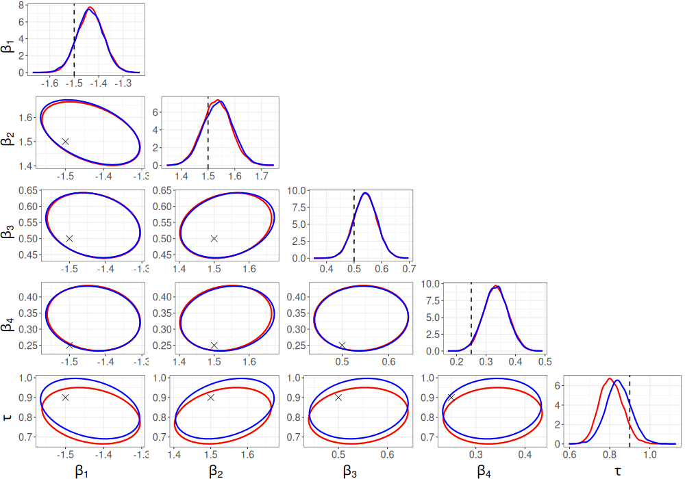
Figure 2: Exact posterior distributions from HMC (in blue) and approximate posterior distributions from R-VGAL with estimated gradients and Hessians (in red) for the logistic mixed model experiment. Diagonal panels: Marginal posterior distributions with true parameters denoted using dotted lines. Off-diagonal panels: Bivariate posterior distributions with true parameters denoted using the symbol $\times$.

3.3 Real data examples

We now apply R-VGAL to two real datasets: the Six City dataset from Fitzmaurice and Laird, (1993), and the POLYPHARMACY dataset from Hosmer et al., (2013).

For the Six City dataset, we follow Tran et al., (2017) and consider the random intercept logistic regression model

$$\log\left(\frac{\pi_{ij}}{1-\pi_{ij}}\right)=\beta_{1}+\beta_{2}\texttt{Age}_{ij}+\beta_{3}\texttt{Smoke}_{ij}+\alpha_{i},\quad\alpha_{i}\sim N(0,\tau^{2}),$$ (19)

where $\pi_{ij}=p(y_{ij}=1\mid\bm{\beta},\tau^{2})$, with $\bm{\beta}=(\beta_{1},\beta_{2},\beta_{3})^{\top}$, for $i=1,\dots,537$ and $j=1,\dots,4$. The binary response variable $y_{ij}=1$ if child $i$ is wheezing at time point $j$, and 0 otherwise. The covariate $\texttt{Age}_{ij}$ is the age of child $i$ at time point $j$, centred at 9 years, while the covariate $\texttt{Smoke}_{ij}=1$ if the mother of child $i$ is smoking at time point $j$, and 0 otherwise. Finally, $\alpha_{i}$ is the random effect associated with the $i$th child. The parameters of the model are $\bm{\theta}=(\bm{\beta}^{\top},\phi_{\tau})^{\top}$, where $\phi_{\tau}=\log(\tau^{2})$.

For the POLYPHARMACY dataset, we consider the random intercept logistic regression model from Tan and Nott, (2018):

$$\log\left(\frac{\pi_{ij}}{1-\pi_{ij}}\right)=\beta_{0} +\beta_{gender}\texttt{Gender}_{i}+\beta_{race}\texttt{Race}_{i}+\beta_{age}\texttt{Age}_{ij}+\beta_{M1}\texttt{MHV1}_{ij}$$

$$+\beta_{M2}\texttt{MHV2}_{ij}+\beta_{M3}\texttt{MHV3}_{ij}+\beta_{IM}\texttt{INPTMHV}_{ij}+\alpha_{i},\quad\alpha_{i}\sim N(0,\tau^{2}),$$ (20)

where $\pi_{ij}=p(y_{ij}=1\mid\bm{\beta},\tau^{2})$, $\bm{\beta}=(\beta_{0},\beta_{gender},\beta_{race},\beta_{age},\beta_{M1},\beta_{M2},\beta_{M3},\beta_{IM})^{\top}$, for $i=1,\dots,500$ and $j=1,\dots,7$. The response variable $y_{ij}$ is 1 if subject $i$ in year $j$ is taking drugs from three or more different classes (of drugs), and 0 otherwise. The covariate $\texttt{Gender}_{i}=1$ if subject $i$ is male, and $0$ if female, while $\texttt{Race}_{i}=0$ if the race of subject $i$ is white, and $1$ otherwise. The covariate $\texttt{Age}_{ij}$ is the age (in years and months, to two decimal places) of subject $i$ in year $j$. The number of outpatient mental health visits (MHV) for subject $i$ in year $j$ is split into three dummy variables: $\texttt{MHV1}_{ij}=1$ if $1\leq\texttt{MHV}_{ij}\leq 5$, and $0$ otherwise; $\texttt{MHV2}_{ij}=1$ if $6\leq\texttt{MHV}_{ij}\leq 14$, and $0$ otherwise; and $\texttt{MHV3}_{ij}=1$ if $\texttt{MHV}_{ij}\geq 15$, and $0$ otherwise. The covariate $\texttt{INPTMHV}_{ij}=0$ if there were no inpatient mental health visits for subject $i$ in year $j$, and $1$ otherwise. Finally, $\alpha_{i}$ is a subject-level random effect for subject $i$. The parameters of the model are $\bm{\theta}=(\bm{\beta}^{\top},\phi_{\tau})^{\top}$, where $\phi_{\tau}=\log(\tau^{2})$.

We use similar priors/initial variational distributions for both examples. For the Six City dataset, the prior/initial variational distribution we use is

$$p(\bm{\theta})=q_{0}(\bm{\theta})=N\left(\begin{bmatrix}\mathbf{0}\\ 1\end{bmatrix},\begin{bmatrix}10\mathbf{I}_{3}&\mathbf{0}\\ \mathbf{0}&1\end{bmatrix}\right),$$ (21)

and for the POLYPHARMACY dataset, we use

$$p(\bm{\theta})=q_{0}(\bm{\theta})=N\left(\begin{bmatrix}\mathbf{0}\\ 1\end{bmatrix},\begin{bmatrix}10\mathbf{I}_{8}&\mathbf{0}\\ \mathbf{0}&1\end{bmatrix}\right).$$ (22)

A $N(1,1)$ prior distribution for $\phi_{\tau}$ is equivalent to a log-normal prior distribution with mean 4.48 and variance 34.51 for $\tau^{2}$. Using this prior distribution, the $2.5$th and $97.5$th percentiles for $\tau^{2}$ are $(0.383,19.297)$, which cover most values of $\tau^{2}$ in practice.

On both datasets, we apply the R-VGAL with tempering algorithm with $n_{temp}=10$ observations and $K=4$ tempering steps per observation. At each R-VGAL iteration, the gradient and Hessian of ${\log p(\mathbf{y}_{i}\mid\bm{\theta})}$ are approximated using $S_{\alpha}=200$ Monte Carlo samples (of $\alpha_{i}$), and the expectations with respect to $q_{i-1}(\bm{\theta})$ in the R-VGAL updates are approximated using $S=200$ Monte Carlo samples (of $\bm{\theta}$).

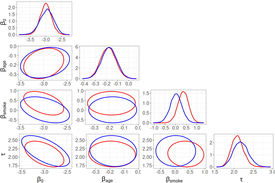
Figure 3: Exact posterior distributions from HMC (in blue) and approximate posterior distributions from R-VGAL with estimated gradients and Hessians (in red) for the experiment with the Six City dataset. Diagonal panels: Marginal posterior distributions. Off-diagonal panels: Bivariate posterior distributions.

Figure 3 shows the marginal posterior distributions of the parameters along with bivariate posterior distributions estimated using R-VGAL and HMC for the Six City dataset. Figure 4 shows the same plots for the POLYPHARMACY dataset. In the Six City example, there is a slight difference in the marginal and bivariate posterior densities from R-VGAL and HMC for the fixed effect $\beta_{smoke}$, but the posterior densities for other parameters are very similar between the two methods. For the POLYPHARMACY example, there are slight differences between the R-VGAL and HMC marginal and bivariate posterior densities for the intercept $\beta_{0}$ and the fixed effects $\beta_{gender}$ and $\beta_{race}$, but for other parameters, the posterior densities are comparable between the two methods.

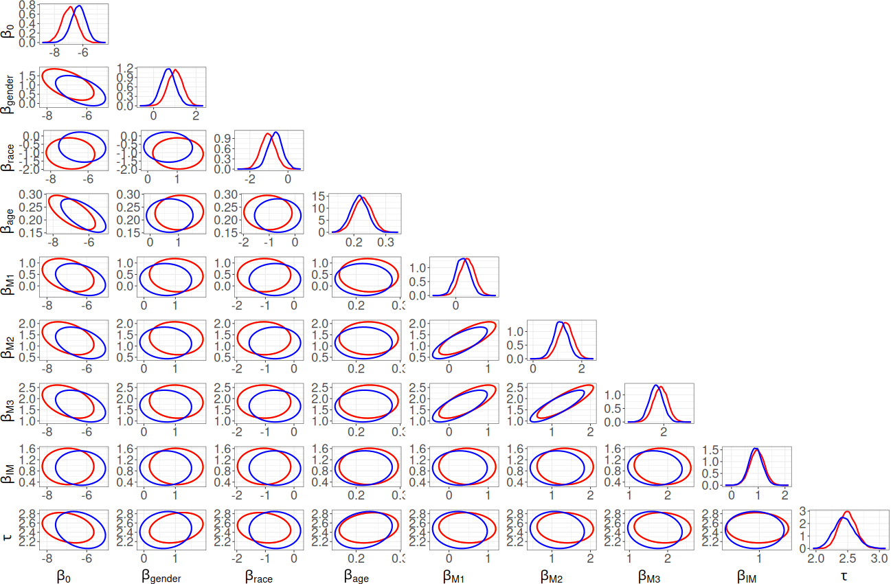
Figure 4: Exact posterior distributions from HMC (in blue) and approximate posterior distributions from R-VGAL with estimated gradients and Hessians (in red) for the experiment with the POLYPHARMACY dataset. Diagonal panels: Marginal posterior distributions. Off-diagonal panels: Bivariate posterior distributions.

Table 1 compares the computing time of R-VGAL and HMC for both simulated and real data examples discussed in this section. The last column shows the average time taken for a single iteration of R-VGAL. For the linear example, where we run R-VGAL with both the theoretical and estimated gradients/Hessians, the displayed time is that of the R-VGAL with the estimated gradients/Hessians. All experiments were carried out on a high-end desktop computer with 64GB of RAM, an Intel^® Core TM i9-7900X CPU, and an NVIDIA^® 1080Ti graphics processing unit (GPU). The table shows that the R-VGAL algorithm is generally 2 to 4 times faster than HMC. In the example with the POLYPHARMACY dataset, where the number of parameters to estimate is highest, R-VGAL is an order of magnitude faster than HMC, which is substantial given that our code is not as highly optimised as that in Stan. Clearly, we can expect R-VGAL to be increasingly useful as the dimensionality of the parameter space increases. Furthermore, since R-VGAL is a sequential algorithm, posterior approximations from R-VGAL can be easily updated as new observations become available. To incorporate an additional observation, R-VGAL need only perform a single update, while an algorithm like HMC requires rerunning from scratch.

	HMC	R-VGAL	R-VGAL (one iteration)
Linear (simulated data)	56	18	0.09
Logistic (simulated data)	181	45	0.09
Logistic (Six City data)	80	51	0.095
Logistic (POLYPHARMACY data)	505	48	0.096

Table 1: The computing time (in seconds) for the R-VGAL and HMC methods for the simulated and real datasets.

4 Conclusion

In this article, we propose a sequential variational Bayes algorithm for estimating parameters in generalised linear mixed models (GLMMs) based on an extension of the R-VGA algorithm of Lambert et al., (2022). The original R-VGA algorithm requires the gradient and Hessian of the partial log-likelihood at each observation, which are computationally intractable for GLMMs. To overcome this, we use Fisher’s and Louis’ identities to obtain unbiased estimates of the gradient and Hessian, which can be used in place of the closed form gradient and Hessian in the R-VGAL algorithm.

We apply R-VGAL to the linear mixed effect and logistic mixed effect models with simulated and real datasets. In all examples, we compare the posterior distributions of the parameters estimated using R-VGAL to those obtained using HMC (Neal,, 2011; Betancourt and Girolami,, 2015). The examples show that R-VGAL yields comparable posterior estimates to HMC while being substantially faster. R-VGAL would be especially useful in situations where new observations are being continuously collected.

In the current paper, we assume that the random effects are independent and identically distributed. Future work will attempt to extend R-VGAL to cases where the random effects are correlated. This will expand the set of models on which R-VGAL can be used to include time series and state space models.

S1 Appendix A: Gradient and Hessian derivations

S1.1 Derivation of gradient and Hessian expressions for the linear mixed model

In the linear mixed model, the theoretical gradient and Hessian for the likelihood at observation $i$ for $i=1,\dots,N$ are available. This section gives the expressions for both the theoretical gradient and Hessian, as well as their approximations when using Fisher’s and Louis’ identities.

S1.1.1 Theoretical gradient and Hessian

The “partial” log-likelihood for observations from the $i$th group is given by

$$\log p(\mathbf{y}_{i}\mid\bm{\theta})=-\frac{n}{2}\log(2\pi)-\frac{1}{2}\log\left\lvert{\mathbf{\Sigma}_{y\mid\theta}}\right\rvert-\frac{1}{2}(\mathbf{y}_{i}-\mathbf{X}_{i}\bm{\beta})^{\top}\mathbf{\Sigma}_{y\mid\theta}^{-1}(\mathbf{y}_{i}-\mathbf{X}_{i}\bm{\beta}),\quad i=1,\dots,N,$$ (S1)

where $\mathbf{\Sigma}_{y\mid\theta}=\exp(\phi_{\alpha})\mathbf{z}_{i}\mathbf{z}_{i}^{\top}+\exp(\phi_{\epsilon})\mathbf{I}_{n}$.

The gradient of the log-likelihood with respect to the parameters $\bm{\theta}$ is given by

$$\nabla_{\bm{\theta}}\log p(\mathbf{y}_{i}\mid\bm{\theta})=(\nabla_{\beta}\log p(\mathbf{y}_{i}\mid\bm{\theta})^{\top},\nabla_{\phi_{\alpha}}\log p(\mathbf{y}_{i}\mid\bm{\theta}),\nabla_{\phi_{\epsilon}}\log p(\mathbf{y}_{i}\mid\bm{\theta}))^{\top},$$

where the components are, respectively,

$$\nabla_{\beta}\log p(\mathbf{y}_{i}\mid\bm{\theta}) =\mathbf{X}_{i}^{\top}\mathbf{\Sigma}_{y\mid\theta}^{-1}(\mathbf{y}_{i}-\mathbf{X}_{i}\bm{\beta})$$ (S2)

$$\nabla_{\phi_{\alpha}}\log p(\mathbf{y}_{i}\mid\bm{\theta}) =-\frac{1}{2}\operatorname{Tr}\left(\mathbf{\Sigma}_{y\mid\theta}^{-1}\frac{\partial\mathbf{\Sigma}_{y\mid\theta}}{\partial\phi_{\alpha}}\right)+\frac{1}{2}(\mathbf{y}_{i}-\mathbf{X}_{i}\bm{\beta})^{\top}\mathbf{\Sigma}_{y\mid\theta}^{-1}\frac{\partial\mathbf{\Sigma}_{y\mid\theta}}{\partial\phi_{\alpha}}\mathbf{\Sigma}_{y\mid\theta}^{-1}(\mathbf{y}_{i}-\mathbf{X}_{i}\bm{\beta})$$ (S3)

$$\nabla_{\phi_{\epsilon}}\log p(\mathbf{y}_{i}\mid\bm{\theta}) =-\frac{1}{2}\operatorname{Tr}\left(\mathbf{\Sigma}_{y\mid\theta}^{-1}\frac{\partial\mathbf{\Sigma}_{y\mid\theta}}{\partial\phi_{\epsilon}}\right)+\frac{1}{2}(\mathbf{y}_{i}-\mathbf{X}_{i}\bm{\beta})^{\top}\mathbf{\Sigma}_{y\mid\theta}^{-1}\frac{\partial\mathbf{\Sigma}_{y\mid\theta}}{\partial\phi_{\epsilon}}\mathbf{\Sigma}_{y\mid\theta}^{-1}(\mathbf{y}_{i}-\mathbf{X}_{i}\bm{\beta}),$$ (S4)

with

$$\frac{\partial\mathbf{\Sigma}_{y\mid\theta}}{\partial\phi_{\alpha}}=\exp(\phi_{\alpha})\mathbf{z}_{i}\mathbf{z}_{i}^{\top},\quad\frac{\partial\mathbf{\Sigma}_{y\mid\theta}}{\partial\phi_{\epsilon}}=\exp(\phi_{\epsilon})\mathbf{I}_{n}.$$ (S5)

The Hessian is given by

$$\nabla^{2}_{\theta}\log p(\mathbf{y}_{i}\mid\bm{\theta})=\begin{bmatrix}\nabla^{2}_{\beta}\log p(\mathbf{y}_{i}\mid\bm{\theta})&\nabla_{\beta}\nabla_{\phi_{\alpha}}\log p(\mathbf{y}_{i}\mid\bm{\theta})&\nabla_{\beta}\nabla_{\phi_{\epsilon}}\log p(\mathbf{y}_{i}\mid\bm{\theta})\\ \nabla_{\beta}\nabla_{\phi_{\alpha}}\log p(\mathbf{y}_{i}\mid\bm{\theta})^{\top}&\nabla^{2}_{\phi_{\alpha}}\log p(\mathbf{y}_{i}\mid\bm{\theta})&\nabla_{\phi_{\alpha}}\nabla_{\phi_{\epsilon}}\log p(\mathbf{y}_{i}\mid\bm{\theta})\\ \nabla_{\beta}\nabla_{\phi_{\epsilon}}\log p(\mathbf{y}_{i}\mid\bm{\theta})^{\top}&\nabla_{\phi_{\alpha}}\nabla_{\phi_{\epsilon}}\log p(\mathbf{y}_{i}\mid\bm{\theta})&\nabla^{2}_{\phi_{\epsilon}}\log p(\mathbf{y}_{i}\mid\bm{\theta})\\ \end{bmatrix}.$$ (S6)

The diagonal terms in the Hessian are the second derivatives

$$\nabla^{2}_{\beta}\log p(\mathbf{y}_{i}\mid\bm{\theta}) =-\mathbf{X}_{i}^{\top}\mathbf{\Sigma}_{y\mid\theta}^{-1}\mathbf{X}_{i},$$ (S7)

$$\nabla^{2}_{\phi_{\alpha}}\log p(\mathbf{y}_{i}\mid\bm{\theta}) =-\frac{1}{2}\operatorname{Tr}(\mathbf{G}_{\phi_{\alpha}})+\frac{1}{2}(\mathbf{y}_{i}-\mathbf{X}_{i}\bm{\beta})^{\top}\mathbf{H}_{\phi_{\alpha}}(\mathbf{y}_{i}-\mathbf{X}_{i}\bm{\beta}),$$ (S8)

where

$$\mathbf{G}_{\phi_{\alpha}} =-\mathbf{\Sigma}_{y\mid\theta}^{-1}\frac{\partial\mathbf{\Sigma}_{y\mid\theta}}{\partial\phi_{\alpha}}\mathbf{\Sigma}_{y\mid\theta}^{-1}\frac{\partial\mathbf{\Sigma}_{y\mid\theta}}{\partial\phi_{\alpha}}+\mathbf{\Sigma}_{y\mid\theta}^{-1}\frac{\partial^{2}\mathbf{\Sigma}_{y\mid\theta}}{\partial\phi_{\alpha}^{2}}$$ (S9)

$$\mathbf{H}_{\phi_{\alpha}} =-2\mathbf{\Sigma}_{y\mid\theta}^{-1}\frac{\partial\mathbf{\Sigma}_{y\mid\theta}}{\partial\phi_{\alpha}}\mathbf{\Sigma}_{y\mid\theta}^{-1}\frac{\partial\mathbf{\Sigma}_{y\mid\theta}}{\partial\phi_{\alpha}}\mathbf{\Sigma}_{y\mid\theta}^{-1}+\mathbf{\Sigma}_{y\mid\theta}^{-1}\frac{\partial^{2}\mathbf{\Sigma}_{y\mid\theta}}{\partial\phi_{\alpha}^{2}}\mathbf{\Sigma}_{y\mid\theta}^{-1},$$ (S10)

with $\frac{\partial^{2}\mathbf{\Sigma}_{y\mid\theta}}{\partial\phi_{\alpha}^{2}}=\exp(\phi_{\alpha})\mathbf{z}_{i}\mathbf{z}_{i}^{\top}$. The expression for $\nabla^{2}_{\phi_{\epsilon}}\log p(\mathbf{y}_{i}\mid\bm{\theta})$ is the same as in (S8), but with all derivatives with respect to $\phi_{\alpha}$ replaced by those with respect to $\phi_{\epsilon}$. Note that $\frac{\partial^{2}\mathbf{\Sigma}_{y\mid\theta}}{\partial\phi_{\epsilon}^{2}}=\exp(\phi_{\epsilon})\mathbf{I}_{n}$.

The off-diagonal terms in the Hessian are

$$\nabla_{\beta}\nabla_{\phi_{\alpha}}\log p(\mathbf{y}_{i}\mid\bm{\theta}) =-\mathbf{X}_{i}^{\top}\mathbf{\Sigma}_{y\mid\theta}^{-1}\frac{\partial\mathbf{\Sigma}_{y\mid\theta}}{\partial\phi_{\alpha}}\mathbf{\Sigma}_{y\mid\theta}^{-1}(\mathbf{y}_{i}-\mathbf{X}_{i}\bm{\beta})$$

$$\nabla_{\beta}\nabla_{\phi_{\epsilon}}\log p(\mathbf{y}_{i}\mid\bm{\theta}) =-\mathbf{X}_{i}^{\top}\mathbf{\Sigma}_{y\mid\theta}^{-1}\frac{\partial\mathbf{\Sigma}_{y\mid\theta}}{\partial\phi_{\epsilon}}\mathbf{\Sigma}_{y\mid\theta}^{-1}(\mathbf{y}_{i}-\mathbf{X}_{i}\bm{\beta})$$

$$\nabla_{\phi_{\alpha}}\nabla_{\phi_{\epsilon}}\log p(\mathbf{y}_{i}\mid\bm{\theta}) =-\frac{1}{2}\operatorname{Tr}(\mathbf{G}_{\phi_{\alpha}\phi_{\epsilon}})+\frac{1}{2}(\mathbf{y}_{i}-\mathbf{X}_{i}\bm{\beta})^{\top}\mathbf{H}_{\phi_{\alpha}\phi_{\epsilon}}(\mathbf{y}_{i}-\mathbf{X}_{i}\bm{\beta}),$$

where

$$\mathbf{G}_{\phi_{\alpha}\phi_{\epsilon}} =-\mathbf{\Sigma}_{y\mid\theta}^{-1}\frac{\partial\mathbf{\Sigma}_{y\mid\theta}}{\partial\phi_{\alpha}}\mathbf{\Sigma}_{y\mid\theta}^{-1}\frac{\partial\mathbf{\Sigma}_{y\mid\theta}}{\partial\phi_{\epsilon}}$$ (S11)

$$\mathbf{H}_{\phi_{\alpha}\phi_{\epsilon}} =-\mathbf{\Sigma}_{y\mid\theta}^{-1}\frac{\partial\mathbf{\Sigma}_{y\mid\theta}}{\partial\phi_{\alpha}}\mathbf{\Sigma}_{y\mid\theta}^{-1}\frac{\partial\mathbf{\Sigma}_{y\mid\theta}}{\partial\phi_{\epsilon}}\mathbf{\Sigma}_{y\mid\theta}^{-1}-\mathbf{\Sigma}_{y\mid\theta}^{-1}\frac{\partial\mathbf{\Sigma}_{y\mid\theta}}{\partial\phi_{\epsilon}}\mathbf{\Sigma}_{y\mid\theta}^{-1}\frac{\partial\mathbf{\Sigma}_{y\mid\theta}}{\partial\phi_{\alpha}}\mathbf{\Sigma}_{y\mid\theta}^{-1}.$$ (S12)

S1.1.2 Expressions for the gradient and Hessian using Fisher’s and Louis’ identities

Fisher’s identity (9) requires the gradient $\nabla_{\theta}\log p(\mathbf{y}_{i},\alpha_{i}\mid\bm{\theta})$, while Louis’ identity (12) requires the Hessian $\nabla_{\theta}^{2}\log p(\mathbf{y}_{i},\alpha_{i}\mid\bm{\theta})$. We now give the expression for these quantities for the linear mixed model considered in Section 3.1.

For $i=1,\dots,N$, the gradient $\nabla_{\theta}\log p(\mathbf{y}_{i},\alpha_{i}\mid\bm{\theta})$ can be written as

$$\nabla_{\theta}\log p(\mathbf{y}_{i},\alpha_{i}\mid\bm{\theta}) =\nabla_{\theta}\log p(\mathbf{y}_{i}\mid\alpha_{i},\bm{\theta})+\nabla_{\theta}\log p(\alpha_{i}\mid\bm{\theta}),$$ (S13)

$$=\nabla_{\theta}\log p(\mathbf{y}_{i}\mid\alpha_{i},\bm{\beta},\phi_{\epsilon})+\nabla_{\theta}\log p(\alpha_{i}\mid\phi_{\alpha}),$$ (S14)

where

$$\log p(\mathbf{y}_{i}\mid\alpha_{i},\bm{\beta},\phi_{\epsilon})=-\frac{n}{2}\log(2\pi)-\frac{1}{2}\log\left\lvert\exp(\phi_{\epsilon})\mathbf{I}_{n}\right\rvert-\frac{1}{2\exp(\phi_{\epsilon})}(\mathbf{y}_{i}-\mathbf{X}_{i}\bm{\beta}-\mathbf{z}_{i}\alpha_{i})^{\top}(\mathbf{y}_{i}-\mathbf{X}_{i}\bm{\beta}-\mathbf{z}_{i}\alpha_{i}),$$ (S15)

and

$$\log p(\alpha_{i}\mid\phi_{\alpha})=-\frac{1}{2}\log(2\pi)-\frac{\phi_{\alpha}}{2}-\frac{\alpha_{i}^{2}}{2\exp(\phi_{\alpha})}.$$ (S16)

Thus, the gradient of the joint $\nabla_{\theta}\log p(\mathbf{y}_{i},\alpha_{i}\mid\bm{\theta})$ is

$$\nabla_{\theta}\log p(\mathbf{y}_{i},\alpha_{i}\mid\bm{\theta})=\left(\nabla_{\beta}\log p(\mathbf{y}_{i},\alpha_{i}\mid\bm{\theta})^{\top},\nabla_{\phi_{\alpha}}\log p(\mathbf{y}_{i},\alpha_{i}\mid\bm{\theta}),\nabla_{\phi_{\epsilon}}\log p(\mathbf{y}_{i},\alpha_{i}\mid\bm{\theta})\right)^{\top},$$ (S17)

where each component is given by

$$\nabla_{\beta}\log p(\mathbf{y}_{i},\alpha_{i}\mid\bm{\theta}) =\nabla_{\beta}\log p(\mathbf{y}_{i}\mid\alpha_{i},\bm{\beta},\phi_{\epsilon})$$

$$=\frac{1}{\exp(\phi_{\epsilon})}\mathbf{X}_{i}^{\top}(\mathbf{y}_{i}-\mathbf{X}_{i}\bm{\beta}-\mathbf{z}_{i}\alpha_{i}),$$ (S18)

$$\nabla_{\phi_{\alpha}}\log p(\mathbf{y}_{i},\alpha_{i}\mid\bm{\theta}) =\nabla_{\phi_{\alpha}}\log p(\alpha_{i}\mid\phi_{\alpha})$$

$$=-\frac{1}{2}+\frac{\alpha_{i}^{2}}{2\exp(\phi_{\alpha})},$$ (S19)

$$\nabla_{\phi_{\epsilon}}\log p(\mathbf{y}_{i},\alpha_{i}\mid\bm{\theta}) =\nabla_{\phi_{\epsilon}}\log p(\mathbf{y}_{i}\mid\alpha_{i},\bm{\beta},\phi_{\epsilon})$$

$$=-\frac{n}{2}+\frac{1}{2\exp(\phi_{\epsilon})}(\mathbf{y}_{i}-\mathbf{X}_{i}\bm{\beta}-\mathbf{z}_{i}\alpha_{i})^{\top}(\mathbf{y}_{i}-\mathbf{X}_{i}\bm{\beta}-\mathbf{z}_{i}\alpha_{i}).$$ (S20)

Similarly, the approximation of the Hessian using Louis’ identity requires $\nabla^{2}_{\theta}\log p(\mathbf{y}_{i},\alpha_{i}\mid\bm{\theta})$, in particular,

$$\nabla^{2}_{\theta}\log p(\mathbf{y}_{i},\alpha_{i}\mid\bm{\theta})=\begin{bmatrix}\nabla^{2}_{\beta}\log p(\mathbf{y}_{i},\alpha_{i}\mid\bm{\theta})&\nabla_{\beta}\nabla_{\phi_{\alpha}}\log p(\mathbf{y}_{i},\alpha_{i}\mid\bm{\theta})&\nabla_{\beta}\nabla_{\phi_{\epsilon}}\log p(\mathbf{y}_{i},\alpha_{i}\mid\bm{\theta})\\ \nabla_{\beta}\nabla_{\phi_{\alpha}}\log p(\mathbf{y}_{i},\alpha_{i}\mid\bm{\theta})^{\top}&\nabla^{2}_{\phi_{\alpha}}\log p(\mathbf{y}_{i},\alpha_{i}\mid\bm{\theta})&\nabla_{\phi_{\alpha}}\nabla_{\phi_{\epsilon}}\log p(\mathbf{y}_{i},\alpha_{i}\mid\bm{\theta})\\ \nabla_{\beta}\nabla_{\phi_{\epsilon}}\log p(\mathbf{y}_{i},\alpha_{i}\mid\bm{\theta})^{\top}&\nabla_{\phi_{\alpha}}\nabla_{\phi_{\epsilon}}\log p(\mathbf{y}_{i},\alpha_{i}\mid\bm{\theta})^{\top}&\nabla^{2}_{\phi_{\epsilon}}\log p(\mathbf{y}_{i},\alpha_{i}\mid\bm{\theta})\\ \end{bmatrix}.$$ (S21)

The components of (S21) are given by

$$\nabla^{2}_{\beta}\log p(\mathbf{y}_{i},\alpha_{i}\mid\bm{\theta}) =-\frac{1}{\exp(\phi_{\epsilon})}\mathbf{X}_{i}^{\top}\mathbf{X}_{i},$$ (S22)

$$\nabla^{2}_{\phi_{\alpha}}\log p(\mathbf{y}_{i},\alpha_{i}\mid\bm{\theta}) =-\frac{\alpha_{i}^{2}}{2\exp(\phi_{\alpha})},$$ (S23)

$$\nabla^{2}_{\phi_{\epsilon}}\log p(\mathbf{y}_{i},\alpha_{i}\mid\bm{\theta}) =-\frac{1}{2\exp(\phi_{\epsilon})}(\mathbf{y}_{i}-\mathbf{X}_{i}\bm{\beta}-\mathbf{z}_{i}\alpha_{i})^{\top}(\mathbf{y}_{i}-\mathbf{X}_{i}\bm{\beta}-\mathbf{z}_{i}\alpha_{i}),$$ (S24)

$$\nabla_{\beta}\nabla_{\phi_{\alpha}}\log p(\mathbf{y}_{i},\alpha_{i}\mid\bm{\theta}) =0,$$ (S25)

$$\nabla_{\beta}\nabla_{\phi_{\epsilon}}\log p(\mathbf{y}_{i},\alpha_{i}\mid\bm{\theta}) =-\frac{1}{\exp(\phi_{\epsilon})}\mathbf{X}_{i}^{\top}(\mathbf{y}_{i}-\mathbf{X}_{i}\bm{\beta}-\mathbf{z}_{i}\alpha_{i}),$$ (S26)

$$\nabla_{\phi_{\alpha}}\nabla_{\phi_{\epsilon}}\log p(\mathbf{y}_{i},\alpha_{i}\mid\bm{\theta}) =0.$$ (S27)

S1.2 Derivation of gradient and Hessian expressions for the logistic mixed model

The parameters of interest are $\bm{\theta}=(\bm{\beta}^{\top},\phi_{\tau})^{\top}$, where $\phi_{\tau}=\log(\tau^{2})$. The likelihood function $p(\mathbf{y}_{i}\mid\bm{\theta})$ is not available in closed form for this model, so the gradient and Hessian of the log likelihood with respect to the parameters $\bm{\theta}$ need to be approximated via Fisher’s and Louis’ identities.

The evaluation of Fisher’s identity requires the gradient $\nabla_{\theta}\log p(\mathbf{y}_{i},\alpha_{i}\mid\bm{\theta})$, where

$$\log p(\mathbf{y}_{i},\alpha_{i}\mid\bm{\theta}) =\log p(\mathbf{y}_{i}\mid\alpha_{i},\bm{\theta})+\log p(\alpha_{i}\mid\bm{\theta})$$

$$=\log p(\mathbf{y}_{i}\mid\alpha_{i},\bm{\beta})+\log p(\alpha_{i}\mid\phi_{\tau}).$$

Individually,

$$\log p(\mathbf{y}_{i}\mid\alpha_{i},\bm{\beta})=\sum_{j=1}^{n}y_{ij}\log\left(\frac{1}{1+\exp(-(\mathbf{x}_{ij}^{\top}\bm{\beta}+\alpha_{i}))}\right)+(1-y_{ij})\log\left(1-\frac{1}{1+\exp(-(\mathbf{x}_{ij}^{\top}\bm{\beta}+\alpha_{i}))}\right)$$

and

$$\log p(\alpha_{i}\mid\phi_{\tau})=-\frac{1}{2}\log(2\pi)-\frac{\phi_{\tau}}{2}-\frac{1}{2}\frac{\alpha_{i}^{2}}{\exp(\phi_{\tau})}.$$

The components of $\nabla_{\theta}\log p(\mathbf{y}_{i},\alpha_{i}\mid\bm{\theta})=(\nabla_{\beta}\log p(\mathbf{y}_{i},\alpha_{i}\mid\bm{\theta})^{\top},\nabla_{\phi_{\tau}}\log p(\mathbf{y}_{i},\alpha_{i}\mid\bm{\theta}))^{\top}$ are derived below:

$$\nabla_{\beta}\log p(\mathbf{y}_{i},\alpha_{i}\mid\bm{\theta}) =\nabla_{\beta}\log p(\mathbf{y}_{i}\mid\alpha_{i},\bm{\beta})\quad\text{(since $\log p(\alpha_{i}\mid\bm{\theta})$ does not depend on $\bm{\beta}$)}$$

$$=\sum_{j=1}^{n}y_{ij}[1+\exp(-(\mathbf{x}_{ij}^{\top}\bm{\beta}+\alpha_{i}))]\frac{\partial}{\partial\bm{\beta}}\left(\frac{1}{1+\exp(-(\mathbf{x}_{ij}^{\top}\bm{\beta}+\alpha_{i}))}\right)$$

$$\quad-\sum_{j=1}^{n}(1-y_{ij})\frac{1+\exp(-(\mathbf{x}_{ij}^{\top}\bm{\beta}+\alpha_{i}))}{\exp(-(\mathbf{x}_{ij}^{\top}\bm{\beta}+\alpha_{i}))}\frac{\partial}{\partial\bm{\beta}}\left(\frac{1}{1+\exp(-(\mathbf{x}_{ij}^{\top}\bm{\beta}+\alpha_{i}))}\right),$$ (S28)

where

$$\frac{\partial}{\partial\bm{\beta}}\left(\frac{1}{1+\exp(-(\mathbf{x}_{ij}^{\top}\bm{\beta}+\alpha_{i}))}\right)=\mathbf{x}_{ij}\frac{\exp(-(\mathbf{x}_{ij}^{\top}\bm{\beta}+\alpha_{i}))}{[1+\exp(-(\mathbf{x}_{ij}^{\top}\bm{\beta}+\alpha_{i}))]^{2}}.$$ (S29)

Substituting (S29) into (S28) and reducing terms gives

$$\nabla_{\beta}\log p(\mathbf{y}_{i},\alpha_{i}\mid\bm{\theta}) =\sum_{j=1}^{n}y_{ij}\mathbf{x}_{ij}\frac{\exp(-(\mathbf{x}_{ij}^{\top}\bm{\beta}+\alpha_{i}))}{1+\exp(-(\mathbf{x}_{ij}^{\top}\bm{\beta}+\alpha_{i}))}-\sum_{j=1}^{n}(1-y_{ij})\mathbf{x}_{ij}\frac{1}{1+\exp(-(\mathbf{x}_{ij}^{\top}\bm{\beta}+\alpha_{i}))}$$ (S30)

$$=\sum_{j=1}^{n}\mathbf{x}_{ij}\left[y_{ij}-\frac{1}{1+\exp(-(\mathbf{x}_{ij}^{\top}\bm{\beta}+\alpha_{i}))}\right].$$ (S31)

The other component of $\nabla_{\theta}\log p(\mathbf{y}_{i},\alpha_{i}\mid\bm{\theta})$ is

$$\nabla_{\phi_{\tau}}\log p(\mathbf{y}_{i},\alpha_{i}\mid\bm{\theta}) =\nabla_{\phi_{\tau}}\log p(\alpha_{i}\mid\phi_{\tau})\quad\text{(since $\log p(\mathbf{y}_{i}\mid\alpha_{i},\bm{\beta})$ does not depend on $\phi_{\tau}$)}$$

$$=-\frac{1}{2}+\frac{\alpha_{i}^{2}}{2\exp(\phi_{\tau})}.$$ (S32)

Evaluation of Louis’ identity similarly requires

$$\nabla^{2}_{\theta}\log p(\mathbf{y}_{i},\alpha_{i}\mid\bm{\theta})=\begin{bmatrix}\nabla^{2}_{\beta}\log p(\mathbf{y}_{i},\alpha_{i}\mid\bm{\theta})&\nabla_{\beta}\nabla_{\phi_{\tau}}\log p(\mathbf{y}_{i},\alpha_{i}\mid\bm{\theta})\\ \nabla_{\beta}\nabla_{\phi_{\tau}}\log p(\mathbf{y}_{i},\alpha_{i}\mid\bm{\theta})^{\top}&\nabla^{2}_{\phi_{\tau}}\log p(\mathbf{y}_{i},\alpha_{i}\mid\bm{\theta})\end{bmatrix},$$ (S33)

the components of which are

$$\nabla^{2}_{\beta}\log p(\mathbf{y}_{i},\alpha_{i}\mid\bm{\theta}) =\sum_{j=1}^{n}\frac{\partial}{\partial\bm{\beta}^{\top}}\left(\frac{\mathbf{x}_{ij}}{1+\exp(-(\mathbf{x}_{ij}^{\top}\bm{\beta}+\alpha_{i}))}\right)=-\sum_{j=1}^{n}\mathbf{x}_{ij}\mathbf{x}_{ij}^{\top}\frac{\exp(-(\mathbf{x}_{ij}^{\top}\bm{\beta}+\alpha_{i}))}{\left[1+\exp(-(\mathbf{x}_{ij}^{\top}\bm{\beta}+\alpha_{i}))\right]^{2}},$$ (S34)

$$\nabla^{2}_{\phi_{\tau}}\log p(\mathbf{y}_{i},\alpha_{i}\mid\bm{\theta}) =-\frac{\alpha_{i}^{2}}{2\exp(\phi_{\tau})},$$ (S35)

$$\nabla_{\beta}\nabla_{\phi_{\tau}}\log p(\mathbf{y}_{i},\alpha_{i}\mid\bm{\theta}) =0.$$ (S36)

S2 Variance of the R-VGAL posterior densities for various Monte Carlo sample sizes

In this section, we study the effects of increasing the number of samples $S$, for estimating the expectations in the variational mean and precision matrix updates, and $S_{\alpha}$, for estimating the gradient of the log-likelihood on the R-VGAL posterior estimates. The results are obtained using the simulated logistic data in Section 3.2 and the POLYPHARMACY dataset in Section 3.3 of the main paper. Similar results are obtained for other datasets. For all simulations in this section, we use the R-VGAL with variational tempering algorithm in Section 2.4 with $n_{temp}=10$ observations and $K=4$ tempering steps per observation.

S2.1 Simulated logistic data

The simulated data used in this section is the same as that used in Section 3.2 of the main paper. The same values for $S$ and $S_{\alpha}$ are used and they are taken from the set $\{50,100,500,1000\}$. For each pair of $S$ and $S_{\alpha}$ values, we independently run R-VGAL 10 times on the simulated dataset, and plot the posterior densities from all 10 runs for each parameter. These posterior densities are shown in Figures S1 to S4. For comparison, the HMC posterior distributions (from a single run) are also plotted in each figure.

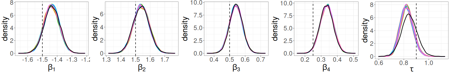
Figure S1: R-VGAL posterior distributions from 10 runs on simulated logistic data are plotted in colour. The Monte Carlo sample sizes are $S=50,S_{\alpha}=50$. HMC posterior distribution are plotted in black for comparison.

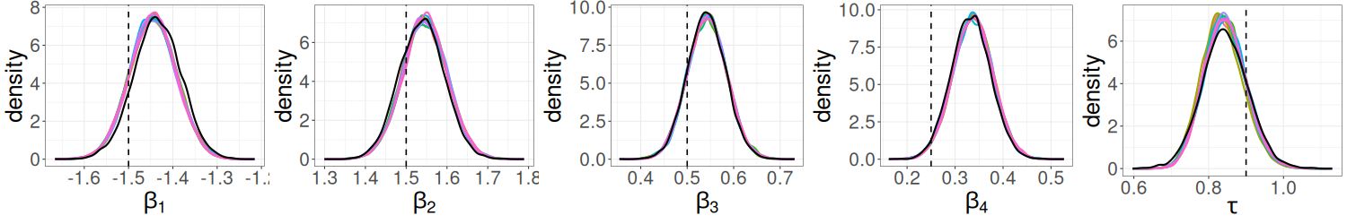
Figure S2: R-VGAL posterior distributions from 10 runs on simulated logistic data are plotted in colour. The Monte Carlo sample sizes are $S=100,S_{\alpha}=100$. HMC posterior distribution are plotted in black for comparison.

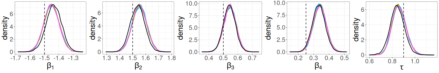
Figure S3: R-VGAL posterior distributions from 10 runs on simulated logistic data are plotted in colour. The Monte Carlo sample sizes are $S=500,S_{\alpha}=500$. HMC posterior distribution are plotted in black for comparison.

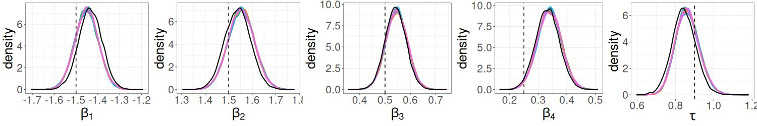
Figure S4: R-VGAL posterior distributions from 10 runs on simulated logistic data are plotted in colour. The Monte Carlo sample sizes are $S=1000,S_{\alpha}=1000$. HMC posterior distribution are plotted in black for comparison.

As the Monte Carlo sample sizes increase, the R-VGAL posterior density estimates get closer and closer to each other, which shows that increasing the values of $S$ and $S_{\alpha}$ helps reduce the variability of the R-VGAL posterior estimates across multiple independent runs.

S2.2 POLYPHARMACY dataset

The POLYPHARMACY dataset used in this section is the same as that used in Section 3.3 of the main paper. Similar to Section S2.1, the same values for $S$ and $S_{\alpha}$ are used and they are taken from the set $\{50,100,500,1000\}$. We independently run R-VGAL 10 times on the POLYPHARMACY dataset for each pair of $S$ and $S_{\alpha}$ values, and plot the posterior densities from all 10 runs for each parameter. For comparison, the HMC posterior distributions (from a single run) are also plotted.

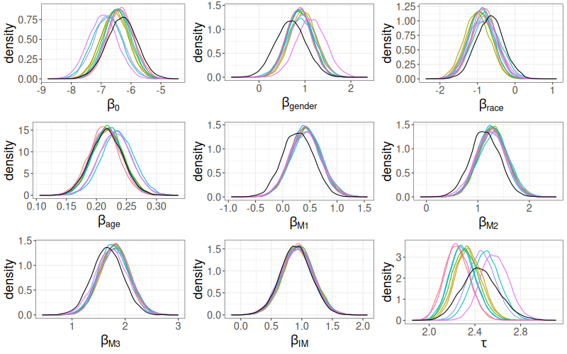
Figure S5: R-VGAL posterior distributions from 10 runs on the POLYPHARMACY dataset are plotted in colour. Tempering is done on the first 10 observations, and the Monte Carlo sample sizes are $S=50,S_{\alpha}=50$. HMC posterior distributions are plotted in black for comparison.

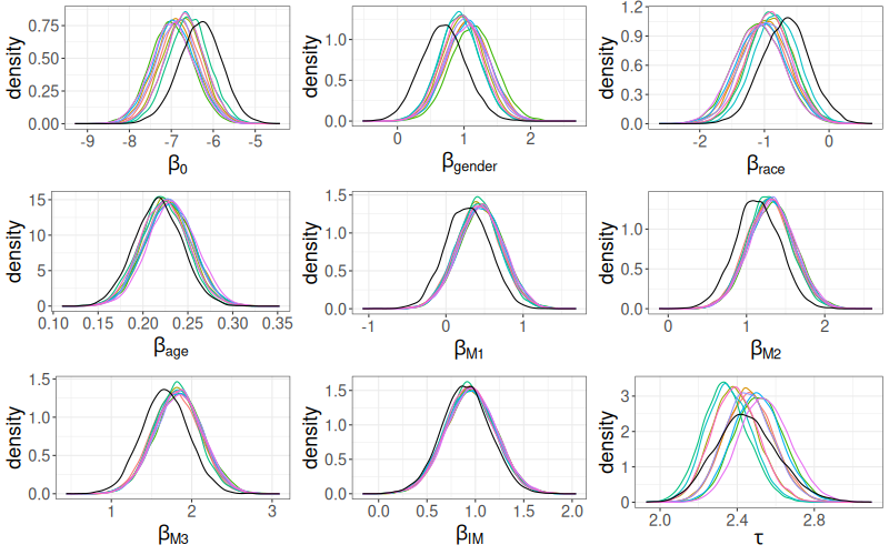
Figure S6: R-VGAL posterior distributions from 10 runs on the POLYPHARMACY dataset are plotted in colour. Tempering is done on the first 10 observations, and the Monte Carlo sample sizes are $S=100,S_{\alpha}=100$. HMC posterior distributions are plotted in black for comparison.

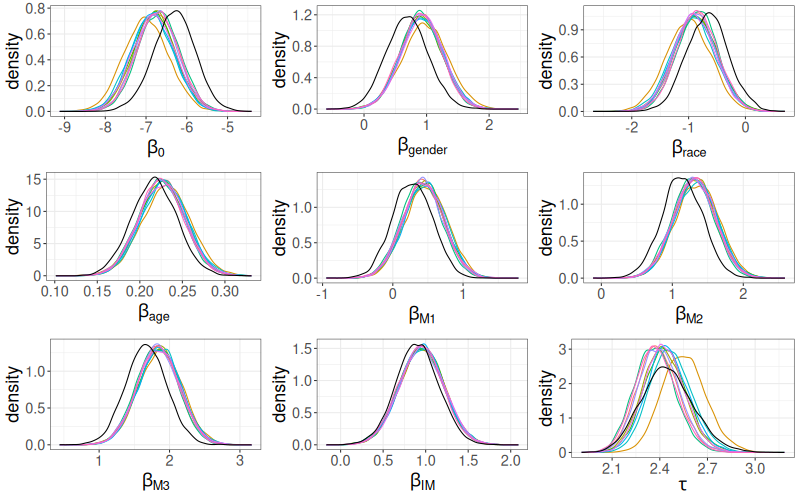
Figure S7: R-VGAL posterior distributions from 10 runs on the POLYPHARMACY dataset are plotted in colour. Tempering is done on the first 10 observations, and the Monte Carlo sample sizes are $S=500,S_{\alpha}=500$. HMC posterior distributions are plotted in black for comparison.

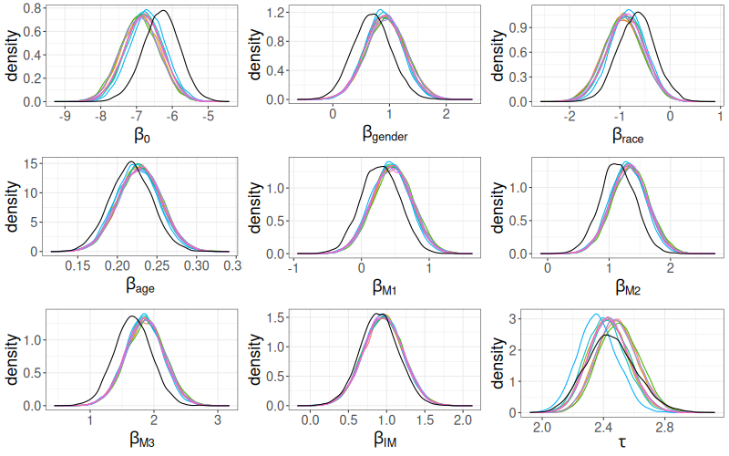
Figure S8: R-VGAL posterior distributions from 10 runs on the POLYPHARMACY dataset are plotted in colour. Tempering is done on the first 10 observations, and the Monte Carlo sample sizes are $S=1000,S_{\alpha}=1000$. HMC posterior distributions are plotted in black for comparison.

As with the previous example, the results in this example also show that increasing the values of $S$ and $S_{\alpha}$ reduces the variability of the R-VGAL posterior estimates across multiple runs. This phenomenon is particularly pronounced for the random effect standard deviation $\tau$. Suitable values for $S$ and $S_{\alpha}$ are likely to be application-dependent. However, from our studies, we conclude that $S$ and $S_{\alpha}$ need to be at least 100 for the Monte Carlo sample sizes not to have a substantial effect on the final estimates.

S3 Robustness check of the R-VGAL algorithm

In this section, we use the POLYPHARMACY dataset in Section 3.3 to check the robustness of the R-VGAL algorithm given different orderings of the data. The simulations in this section show that R-VGAL can be unstable while traversing the first few observations, which makes it sensitive to the ordering of observations. This instability can, however, be alleviated with variational tempering, as described in Section 2.4 of the main paper.

Figures S9 and S10 show the R-VGAL posterior density estimates from 10 independent runs using the original ordering of the data and a random ordering of the data, respectively. In both simulations, the number of Monte Carlo samples $S$ to estimate the expectation with respect to $q_{i-1}(\bm{\theta})$ and the number of samples $S_{\alpha}$ to estimate the gradients/Hessians are fixed to $100$. In both figures, the HMC posterior densities for each parameter are plotted in black for comparison. The figures show that the R-VGA estimates are quite far away from those of HMC estimates when using the original ordering of the data, while the R-VGA estimates are reasonably close to those of HMC when using the random ordering of the data. This suggests that the R-VGAL estimates are not robust with respect to the ordering of the data.

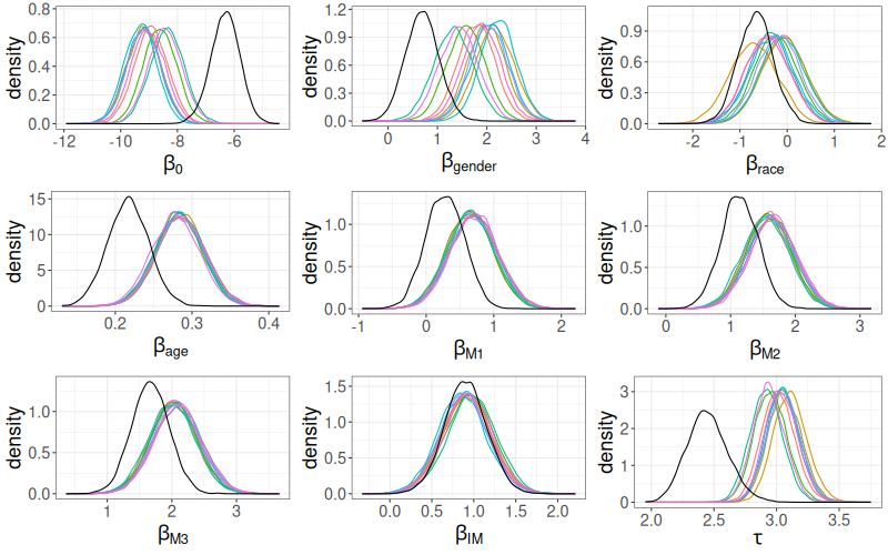
Figure S9: R-VGAL posterior distributions from 10 independent runs using the original ordering of the data are plotted in different colours. The Monte Carlo sample sizes are $S=100,S_{\alpha}=100$. HMC posterior distributions are plotted in black for comparison.

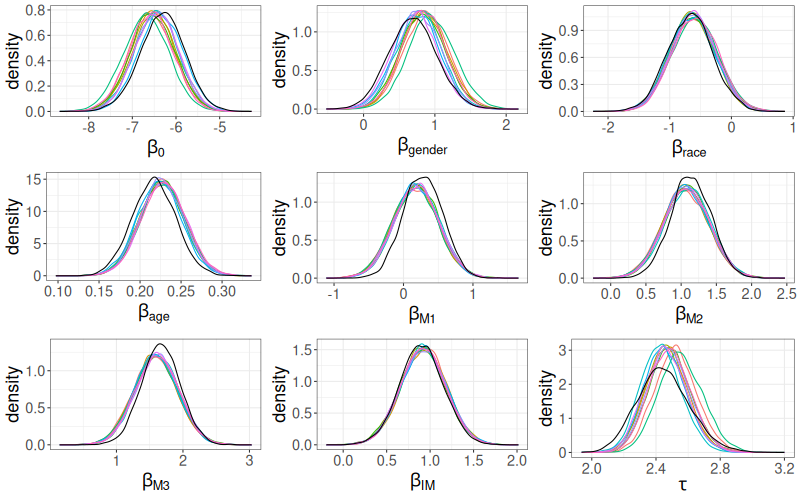
Figure S10: R-VGAL posterior distributions from 10 independent runs using the random ordering of the data are plotted in different colours. The Monte Carlo sample sizes are $S=100$, and $S_{\alpha}=100$. HMC posterior distributions are plotted in black for comparison.

To confirm that the source of variability in the R-VGAL estimates is from different data orderings and not from the low number of Monte Carlo samples, we increase the number of Monte Carlo samples $S$ and $S_{\alpha}$. Figures S11 and S12 show the R-VGAL posterior density estimates from 10 independent runs using the original ordering of the data and a random ordering of the data, respectively, with the Monte Carlo sample sizes set to $S=S_{\alpha}=1000$. The posterior densities for each parameter are different for the two orderings; for instance, with the original ordering, the posterior of $\tau$ is centred around 4.5, while with the random ordering, the posterior of $\tau$ is centred around 2.4.

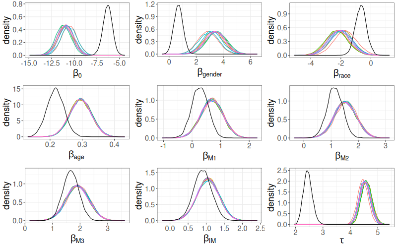
Figure S11: R-VGAL posterior distributions from 10 independent runs using the original ordering of the data are plotted in colour. The Monte Carlo sample sizes are $S=1000,S_{\alpha}=1000$. HMC posterior distributions are plotted in black for comparison.

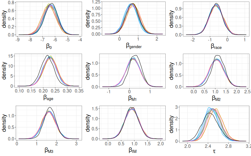
Figure S12: R-VGAL posterior distributions from 10 independent runs using the random ordering of the data are plotted in colour. The Monte Carlo sample sizes are $S=1000,S_{\alpha}=1000$. HMC posterior distributions are plotted in black for comparison.

A plot of the trajectory of the variational mean across R-VGAL iterations reveals that R-VGAL is unstable during the first few iterations. The blue lines in Figures S13 and S14 show the trajectories of the variational mean for each of the parameters across 10 independent runs of the R-VGAL algorithm, on the original ordering and on a random ordering of the data, respectively. The initial trajectories of the fixed effect parameters in Figure S13 vary significantly (for example, between -50 and 0 for the intercept $\beta_{0}$), and the trajectory of $\tau$ is dragged up to nearly 7 before progressively dropping towards 4. This potentially contributes to the biased posterior mean of $\tau$. In Figure S14, where the data were randomly reordered, the trajectories of the parameters are less variable initially, which then allows the variational mean to converge towards the true values more rapidly. This shows that the R-VGAL algorithm is unstable while traversing the first few observations, making the algorithm sensitive to the ordering of the data.

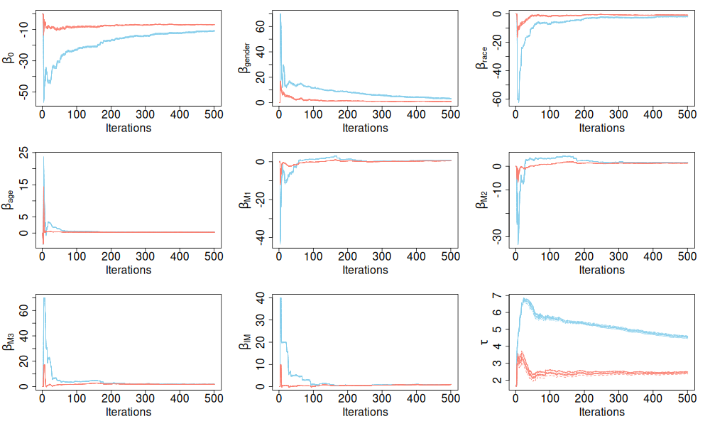
Figure S13: Trajectories of the variational mean without tempering (in blue) and with tempering (in red) for each parameter across 10 independent runs of R-VGAL on the original ordering of the data. The Monte Carlo sample sizes are $S=1000$ and $S_{\alpha}=1000$.

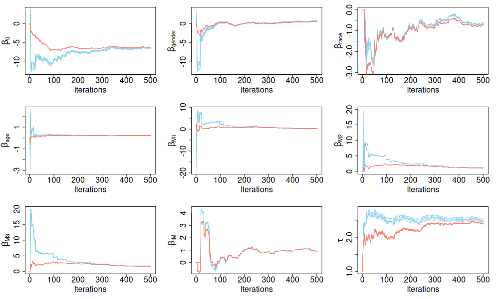
Figure S14: Trajectories of the variational mean without tempering (in blue) and with tempering (in red) for each parameter across 10 independent runs of R-VGAL on the random ordering of the data. The Monte Carlo sample sizes are $S=1000$ and $S_{\alpha}=1000$.

We propose a tempering approach (in Section 2.4 of the main paper) to make the R-VGAL algorithm more robust. By tempering the first few observations, the R-VGAL posterior estimates become much more consistent across different data orderings. Figures S15 and S16 show the posterior density estimates from 10 independent runs of the R-VGAL algorithm using the original ordering of the data and a random ordering of the data, respectively, with tempering done on the first 10 observations. These figures show that the posterior density estimates of R-VGAL with tempering are consistent across two different orderings of the data, and also consistent with those obtained from HMC.

Figure S15: R-VGAL posterior distributions from 10 independent runs using the original ordering of the data are plotted in colour. Tempering is done on the first 10 observations. The Monte Carlo sample sizes are $S=100,S_{\alpha}=100$. HMC posterior distributions are plotted in black for comparison.

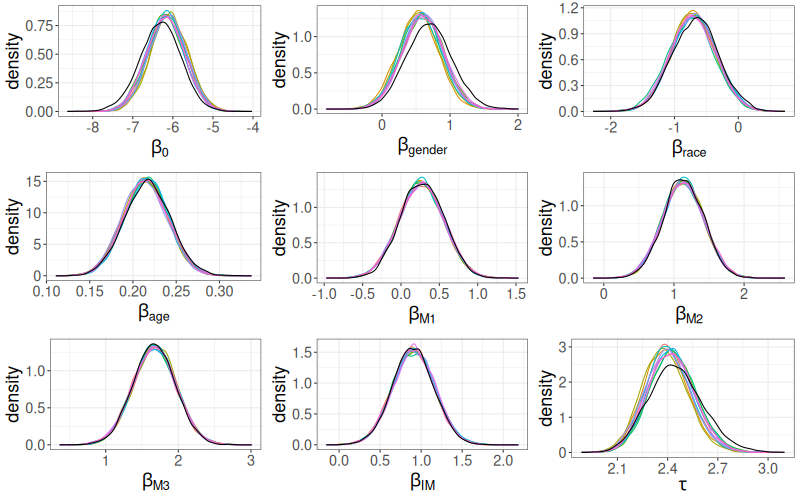
Figure S16: R-VGAL posterior distributions from 10 independent runs using a random reordering of the data are plotted in colour. Tempering is done on the first 10 observations. The Monte Carlo sample sizes are $S=100,S_{\alpha}=100$. HMC posterior distributions are plotted in black for comparison.

Figures S17 and S18 display the R-VGAL posterior densities using the original ordering and the random ordering of the data, respectively, with tempering done on the first 10 observations, and Monte Carlo sample sizes increased to $S=S_{\alpha}=1000$. There is now very little difference between the posterior densities using the original and the random ordering of the dataset. The red lines in Figures S13 and S14 show the parameter trajectories obtained from R-VGAL with tempering, on the original ordering and the random ordering of the data, respectively. The trajectories with tempering (plotted in red) are much more stable than those without tempering (plotted in blue), especially during the first few iterations. These figures suggest that tempering is effective in reducing the variability of R-VGAL estimates while traversing the first few observations and increases the algorithm’s robustness to different data orderings. Other random orderings of the data give similar results.

Figure S17: R-VGAL posterior distributions from 10 independent runs using the original ordering of the data are plotted in colour. Tempering is done on the first 10 observations. The Monte Carlo sample sizes are $S=1000,S_{\alpha}=1000$. HMC posterior distributions are plotted in black for comparison.

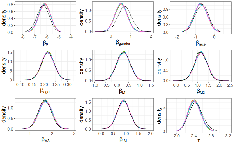
Figure S18: R-VGAL posterior distributions from 10 independent runs using a random reordering of the data are plotted in colour. Tempering is done on the first 10 observations. The Monte Carlo sample sizes are $S=1000,S_{\alpha}=1000$. HMC posterior distributions are plotted in black for comparison.

References

- Betancourt and Girolami, (2015) Betancourt, M. and Girolami, M. (2015). Hamiltonian Monte Carlo for hierarchical models. Current Trends in Bayesian Methodology with Applications, 79(30):2–4.
- Blei et al., (2017) Blei, D. M., Kucukelbir, A., and McAuliffe, J. D. (2017). Variational inference: a review for statisticians. Journal of the American Statistical Association, 112(518):859–877.
- Bottou, (2010) Bottou, L. (2010). Large-scale machine learning with stochastic gradient descent. In Proceedings of COMPSTAT’2010: 19th International Conference on Computational Statistics, pages 177–186. Springer, New York, NY.
- Breslow and Clayton, (1993) Breslow, N. E. and Clayton, D. G. (1993). Approximate inference in generalized linear mixed models. Journal of the American Statistical Association, 88(421):9–25.
- Broderick et al., (2013) Broderick, T., Boyd, N., Wibisono, A., Wilson, A. C., and Jordan, M. I. (2013). Streaming variational Bayes. In Proceedings of the 26th International Conference on Neural Information Processing Systems - Volume 2, NIPS’13, page 1727–1735. Curran Associates Inc., Red Hook, NY.
- Cappé et al., (2005) Cappé, O., Moulines, E., and Rydén, T. (2005). Inference in Hidden Markov Models. Springer, New York, NY.
- Crowder, (1979) Crowder, M. J. (1979). Inference about the intraclass correlation coefficient in the beta-binomial ANOVA for proportions. Journal of the Royal Statistical Society B, 41(2):230–234.
- Dempster et al., (1977) Dempster, A. P., Laird, N. M., and Rubin, D. B. (1977). Maximum likelihood from incomplete data via the EM algorithm. Journal of the Royal Statistical Society B, 39(1):1–22.
- Fitzmaurice and Laird, (1993) Fitzmaurice, G. M. and Laird, N. M. (1993). A likelihood-based method for analysing longitudinal binary responses. Biometrika, 80(1):141–151.
- Fong et al., (2010) Fong, Y., Rue, H., and Wakefield, J. (2010). Bayesian inference for generalized linear mixed models. Biostatistics, 11(3):397–412.
- Gelman et al., (2004) Gelman, A., Carlin, J. B., Stern, H. S., and Rubin, D. B. (2004). Bayesian Data Analysis. CRC Press, New York, NY, 3rd edition.
- Goldstein, (1991) Goldstein, H. (1991). Nonlinear multilevel models, with an application to discrete response data. Biometrika, 78(1):45–51.
- Gunawan et al., (2021) Gunawan, D., Kohn, R., and Nott, D. (2021). Variational Bayes approximation of factor stochastic volatility models. International Journal of Forecasting, 37(4):1355–1375.
- Hoffman et al., (2013) Hoffman, M. D., Blei, D. M., Wang, C., and Paisley, J. (2013). Stochastic variational inference. Journal of Machine Learning Research, 14:1303–1347.
- Hosmer et al., (2013) Hosmer, D. W., Lemeshow, S., and Sturdivant, R. X. (2013). Applied Logistic Regression. John Wiley & Sons, Hoboken, NJ, 3rd edition.
- Huang et al., (2018) Huang, C.-W., Tan, S., Lacoste, A., and Courville, A. C. (2018). Improving explorability in variational inference with annealed variational objectives. In Bengio, S., Wallach, H., Larochelle, H., Grauman, K., Cesa-Bianchi, N., and Garnett, R., editors, Advances in Neural Information Processing Systems, volume 31. Curran Associates, Inc., Red Hook, NY.
- Jansen, (1994) Jansen, M. G. H. (1994). Parameters of the latent distribution in Rasch’s Poisson counts model. In Fischer, G. H. and Laming, D., editors, Contributions to Mathematical Psychology, Psychometrics, and Methodology, pages 319–326. Springer, New York, NY.
- Kingma and Welling, (2013) Kingma, D. P. and Welling, M. (2013). Auto-encoding variational Bayes. arXiv preprint arXiv:1312.6114.
- Lambert et al., (2022) Lambert, M., Bonnabel, S., and Bach, F. (2022). The recursive variational Gaussian approximation (R-VGA). Statistics and Computing, 32(10).
- Mandt et al., (2016) Mandt, S., McInerney, J., Abrol, F., Ranganath, R., and Blei, D. (2016). Variational tempering. In Gretton, A. and Robert, C. C., editors, Proceedings of the 19th International Conference on Artificial Intelligence and Statistics, volume 51 of Proceedings of Machine Learning Research, pages 704–712. PMLR, Cadiz, Spain.
- Naylor and Smith, (1982) Naylor, J. C. and Smith, A. F. (1982). Applications of a method for the efficient computation of posterior distributions. Journal of the Royal Statistical Society C, 31(3):214–225.
- Neal, (2011) Neal, R. (2011). MCMC using Hamiltonian dynamics. In Brooks, S., Gelman, A., Jones, G. J., and Meng, X.-L., editors, Handbook of Markov Chain Monte Carlo. CRC Press, Boca Raton, FL.
- Nemeth et al., (2016) Nemeth, C., Fearnhead, P., and Mihaylova, L. (2016). Particle approximations of the score and observed information matrix for parameter estimation in state–space models with linear computational cost. Journal of Computational and Graphical Statistics, 25(4):1138–1157.
- Ong et al., (2018) Ong, V. M.-H., Nott, D. J., and Smith, M. S. (2018). Gaussian variational approximation with a factor covariance structure. Journal of Computational and Graphical Statistics, 27(3):465–478.
- Ormerod and Wand, (2010) Ormerod, J. T. and Wand, M. P. (2010). Explaining variational approximations. The American Statistician, 64(2):140–153.
- R Core Team, (2022) R Core Team (2022). R: A Language and Environment for Statistical Computing. R Foundation for Statistical Computing, Vienna, Austria.
- Stan Development Team, (2023) Stan Development Team (2023). RStan: the R interface to Stan. R package version 2.21.8.
- Tan and Nott, (2018) Tan, L. S. and Nott, D. J. (2018). Gaussian variational approximation with sparse precision matrices. Statistics and Computing, 28(2018):259–275.
- Tierney and Kadane, (1986) Tierney, L. and Kadane, J. B. (1986). Accurate approximations for posterior moments and marginal densities. Journal of the American Statistical Association, 81(393):82–86.
- Tomasetti et al., (2022) Tomasetti, N., Forbes, C., and Panagiotelis, A. (2022). Updating variational Bayes: Fast sequential posterior inference. Statistics and Computing, 32(1).
- Tran et al., (2017) Tran, M.-N., Nott, D. J., and Kohn, R. (2017). Variational Bayes with intractable likelihood. Journal of Computational and Graphical Statistics, 26(4):873–882.
- Tran et al., (2016) Tran, M.-N., Nott, D. J., Kuk, A. Y., and Kohn, R. (2016). Parallel variational Bayes for large datasets with an application to generalized linear mixed models. Journal of Computational and Graphical Statistics, 25(2):626–646.
- Tuerlinckx et al., (2006) Tuerlinckx, F., Rijmen, F., Verbeke, G., and De Boeck, P. (2006). Statistical inference in generalized linear mixed models: A review. British Journal of Mathematical and Statistical Psychology, 59(2):225–255.
- Verbeke et al., (1997) Verbeke, G., Molenberghs, G., and Verbeke, G. (1997). Linear Mixed Models for Longitudinal Data. Springer, New York, NY.
- Wakefield, (2013) Wakefield, J. (2013). Bayesian and Frequentist Regression Methods. Springer, New York, NY.
- Zhao et al., (2006) Zhao, Y., Staudenmayer, J., Coull, B. A., and Wand, M. P. (2006). General design Bayesian generalized linear mixed models. Statistical Science, 21(1):35–51.