HYSPECNET-11K: A LARGE-SCALE HYPERSPECTRAL DATASET FOR BENCHMARKING LEARNING-BASED HYPERSPECTRAL IMAGE COMPRESSION METHODS

Abstract

The development of learning-based hyperspectral image compression methods has recently attracted great attention in remote sensing. Such methods require a high number of hyperspectral images to be used during training to optimize all parameters and reach a high compression performance. However, existing hyperspectral datasets are not sufficient to train and evaluate learning-based compression methods, which hinders the research in this field. To address this problem, in this paper we present HySpecNet-11k that is a large-scale hyperspectral benchmark dataset made up of $11,483$ nonoverlapping image patches. Each patch is a portion of 128x128 $\mathrm{pixels}$ with $224\text{\,}\mathrm{spectral\ bands}$ and a ground sample distance of $30\text{\,}\mathrm{m}$. We exploit HySpecNet-11k to benchmark the current state of the art in learning-based hyperspectral image compression by focussing our attention on various 1D, 2D and 3D convolutional autoencoder architectures. Nevertheless, HySpecNet-11k can be used for any unsupervised learning task in the framework of hyperspectral image analysis. The dataset, our code and the pre-trained weights are publicly available at https://hyspecnet.rsim.berlin.

Index Terms—  EnMAP, hyperspectral dataset, image compression, deep learning, remote sensing.

1 Introduction

Advancements in hyperspectral imaging technologies have led to a significant increase in the volume of hyperspectral data archives [1]. Dense spectral information provided by hyperspectral images leads to a very high capability for the identification and discrimination of the materials in a given scene. However, to reduce the storage required for the huge amounts of hyperspectral data, it is needed to compress the images before storing them. Accordingly, one emerging research topic is associated to the efficient and effective compression of hyperspectral images [2].

Many HSI compression algorithms are presented in the literature. Generally, they can be divided into two categories: i) traditional methods, e.g. [3, 4, 5]; and ii) learning-based methods, e.g. [6, 7, 8, 9, 10]. The most popular traditional algorithms are defined based on transform coding in combination with a quantization step and entropy coding. In contrast, learning-based methods mostly rely on convolutional autoencoders to reduce the dimensionality of the latent space. Recent studies show that learning-based HSI compression methods can preserve the reconstruction quality at lower rates compared to traditional compression approaches.

Learning-based compression methods generally require a large number of unlabeled images to optimize their model parameters during training. There are only few hyperspectral benchmark datasets publicly available in remote sensing (see Table 1). To the best of our knowledge, most of the existing datasets only contain a single HSI, which is divided into patches for the training and evaluation processes. Thus, they are not sufficient to train learning-based compression methods to reach a high generalization ability as the models may overfit dramatically, when using such training data from spatially joint areas. The lack of a large hyperspectral dataset is an important bottleneck, affecting the research and development in the field of learning-based HSI compression. Hence, a large-scale benchmark archive consisting of a high number of HSIs acquired in spatially disjoint geographical areas is needed.

Table 1: A summary of publicly available hyperspectral benchmark datasets and their characteristics.

Dataset	Acquisition	Sensor	GSD	Spectral Range	#Bands	Dataset Size
Indian Pines	1992	AVIRIS	$20.0\text{\,}\mathrm{m}$	$4002500\text{\,}\mathrm{nm}$	$224$	00$0.021,025\text{\,}\mathrm{MP}$
Kennedy Space Center (KSC)	1996	AVIRIS	$18.0\text{\,}\mathrm{m}$	$4002500\text{\,}\mathrm{nm}$	$224$	00$0.314,368\text{\,}\mathrm{MP}$
Salinas Scene	1998	AVIRIS	0$3.7\text{\,}\mathrm{m}$	$4202450\text{\,}\mathrm{nm}$	$224$	00$0.111,104\text{\,}\mathrm{MP}$
Pavia Center	2001	ROSIS	0$1.3\text{\,}\mathrm{m}$	$430$ – 0$860\text{\,}\mathrm{nm}$	$102$	00$1.201,216\text{\,}\mathrm{MP}$
Pavia University	2001	ROSIS	0$1.3\text{\,}\mathrm{m}$	$430$ – 0$860\text{\,}\mathrm{nm}$	$103$	00$0.2074\text{\,}\mathrm{MP}$
Botswana	2001	Hyperion	$30.0\text{\,}\mathrm{m}$	$4002500\text{\,}\mathrm{nm}$	$242$	00$0.377,856\text{\,}\mathrm{MP}$
Cooke City	2008	HyMap	0$3.0\text{\,}\mathrm{m}$	$4502480\text{\,}\mathrm{nm}$	$126$	00$0.224\text{\,}\mathrm{MP}$
ShanDongFeiCheng (SDFC)	2021	HAHS	0$0.5\text{\,}\mathrm{m}$	$4001000\text{\,}\mathrm{nm}$	0$63$	00$0.721,801\text{\,}\mathrm{MP}$
HySpecNet-11k (ours)	$2022$	EnMAP	$30.0\text{\,}\mathrm{m}$	$4202450\text{\,}\mathrm{nm}$	$224$	$188.137,472\text{\,}\mathrm{MP}$

To address this problem, in this paper we introduce a new hyperspectral benchmark dataset (denoted as HySpecNet-11k) and exploit it to benchmark the current state of the art in learning-based HSI compression.

2 The HySpecNet-11k Dataset

HySpecNet-11k is made up of $11,483$ image patches acquired by the Environmental Mapping and Analysis Program (EnMAP) satellite [11]. Each image patch in HySpecNet-11k consists of 128x128 $\mathrm{pixels}$ and $224\text{\,}\mathrm{bands}$ with a ground sample distance (GSD) of $30\text{\,}\mathrm{m}$ (see Table 1).

To construct HySpecNet-11k, a total of $250$ EnMAP tiles acquired during the routine operation phase between 2 November 2022 and 9 November 2022 were considered. It is worth nothing that the considered tiles are associated with less than $10\text{\,}\mathrm{\char 37\relax}$ cloud and snow cover. The tiles were radiometrically, geometrically and atmospherically corrected (L2A water & land product). Then, the tiles were divided into nonoverlapping image patches. Therefore, cropped patches at the borders of the tiles were eliminated. Thus, we were able to generate more than $45$ patches per tile resulting in an overall number of $11,483$ patches for the full dataset. Due to the L2A-processed data, the number of bands is reduced from $224$ to $202$ by removing bands [$127141\text{\,}$] and [$161167\text{\,}$] that are affected by strong water vapor absorption.

We provide predefined splits to make the results of the considered methods reproducible. Therefore, we randomly divided the dataset into: i) a training set that includes $70\text{\,}\mathrm{\char 37\relax}$ of the patches, ii) a validation set that includes $20\text{\,}\mathrm{\char 37\relax}$ of the patches, and iii) a test set that includes $10\text{\,}\mathrm{\char 37\relax}$ of the patches. Depending on the way that we used for splitting the dataset, we define two different splits: i) an easy split, where patches from the same tile can be present in different sets (patchwise splitting); and ii) a hard split, where all patches from one tile must belong to the same set (tilewise splitting).

To get an overview of the dataset, Figure 1 illustrates representative HySpecNet-11k images patches. It is worth noting that compression methods generally do not require labeled training images and therefore our dataset does not contain image annotations.

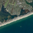
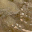
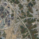
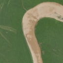
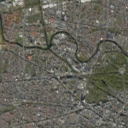
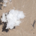
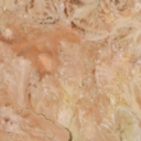
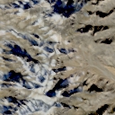
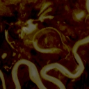
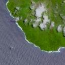
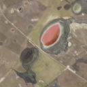
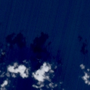
Fig. 1: True color representations of example images from our proposed HySpecNet-11k dataset. Red, green and blue channels are extracted from EnMAP bands $43$, $28$ and $10$ at wavelengths $634.919\text{\,}\mathrm{nm}$, $550.525\text{\,}\mathrm{nm}$ and $463.584\text{\,}\mathrm{nm}$, respectively.

3 Learning-based Hyperspectral Image Compression

In order to provide an initial benchmarking of the proposed HySpecNet-11k dataset in the framework of learning-based HSI compression, we train and evaluate the following state of the art baseline methods: i) 1D-Convolutional Autoencoder(1D-CAE) [6]; ii) Advanced 1D-Convolutional Autoencoder(1D-CAE-Adv) [7]; iii) Extended 1D-Convolutional Autoencoder(1D-CAE-Ext) [8]; iv) Spectral Signals Compressor Network(SSCNet) [9]; and v) 3D Convolutional Auto-Encoder(3D-CAE) [10]. All methods are based on convolutional operations paired with down- and upsamplings in the encoder and decoder, respectively. They differ from each other with respect to the approaches considered for spatial and spectral compression.

An overview of the considered methods is given in the following. For a detailed description we refer the reader to the respective papers.

The 1D-Convolutional Autoencoder (1D-CAE) [6] applies pixelwise compression without utilizing spatial content. The encoder consists of multiple 1D convolutions in combination with two 1D max pooling layers that fix the compression ratio (CR) to a factor of $4$. leakyrelu are present as activation functions after each convolution. The decoder mirrors the encoder, however it uses two upsampling layers to reverse the respective downsamplings from the encoder. A sigmoid activation function scales the reconstructed pixel values to the range from $01\text{\,}$ in the last decoder layer. Furthermore, padding and unpadding are needed in encoder and decoder, respectively. The Advanced 1D-Convolutional Autoencoder (1D-CAE-Adv) [7] adapts the decoder by substituting the combinations of 1D convolutional layer and upsampling layer with 1D transposed convolutions to make the upsampling operation trainable and more adaptive. On the encoder side, the 1D max poolings are dropped for 1D average poolings. Moreover, the Extended 1D-Convolutional Autoencoder (1D-CAE-Ext) [8] adds a 1D batch normalization [12] between each (transposed) convolutional and activation layer. The sigmoid activation in the last decoder layer is replaced by a hard hyperbolic tangent (HardTanh) and 1D average poolings are substituted by 1D max poolings again. The repetition of down- and upsampling blocks enables the construction of models with different CRs.

The Spectral Signals Compressor Network (SSCNet) [9] encoder uses 2D convolutions with parametric rectified linear units as activation after each convolutional layer. Three 2D max pooling layers are added for a fixed spatial compression by a factor of $64$. The final CR is set via the number of latent channels in the bottleneck layer. Simultaneously, the ratio between input and latent channels decides the spectral compression factor. 2D transposed convolutions are used to reconstruct the HSIs on the decoder side. After each transposed convolution there is a PReLU activation except for the last layer where a sigmoid activation is used for scaling the outputs into the correct range from $01\text{\,}$. For all convolutional layers a kernel size of 3x3 $\mathrm{pixels}$ ensures the integration of nearby spatial content into the compression of the currently considered pixel.

The 3D-CAE [10] is built by three strided 3D convolutional layers, each of which is followed by a 3D batch normalization [12] and a leaky rectified linear unit (LeakyReLU). Residual blocks are added to increase the depth of the network. Upsampling layers are furthermore present on the decoder side for reconstruction. Padding operations are required as in the 1D-CAE. The 3D kernels in the convolutional layers are able to integrate the local spatial and spectral neighborhood jointly during the compression. Spatial and spectral CRs are fixed to a factor of $64$ and $4$, respectively and the overall CR can be set via the number of latent channels in the bottleneck of the network.

4 Experimental Results

Our code is implemented in PyTorch based on the CompressAI [13] framework. We applied gradient clipping and a global min-max normalization to scale the input data in the range between $01\text{\,}$ that is usually a requirement for learning-based compression methods. As optimizer, we used Adam [14] with a learning rate of $1\text{\times}{10}^{-4}$ for the 1D-CAE [6], 1D-CAE-Adv [7] and 1D-CAE-Ext [8]. For SSCNet [9] and 3D-CAE [10] the learning rate was set to $1\text{\times}{10}^{-5}$. We trained the networks using mean squared error (MSE) as loss function until convergence on the validation set that took $500\text{\,}\mathrm{epochs}$, $2000\text{\,}\mathrm{epochs}$ and $1000\text{\,}\mathrm{epochs}$ for the 1D-CAEs, SSCNet and 3D-CAE, respectively. Training runs were carried out on a single NVIDIA A100 SXM4 80 GB GPU and took between $110\text{\,}\mathrm{days}$ each, depending on the method. In general, SSCNet requires fewer GPU hours than 1D-CAE and 3D-CAE. For the 1D-CAE another factor is the CR. The higher the CR, the deeper the network and thus the longer the training time. Therefore, the modified versions of the 1D-CAE with increased CRs were trained for only $250\text{\,}\mathrm{epochs}$ due to runtime limitations.

Rate-distortion performance of the baseline methods on the HySpecNet-11k test set is shown in Figure 2. The results have been obtained by using the HySpecNet-11k easy split as introduced in Section 2. Overall, the 1D-CAE produces the highest quality reconstructions with a peak signal-to-noise ratio (PSNR) of $54.847,359,908,951,65\text{\,}\mathrm{dB}$ at a relatively high fixed rate of $8.079,207,921\text{\,}\mathrm{bpppc}$. Despite the added trainable upsampling operations, the 1D-CAE-Adv reaches a $0.662,468,817\text{\,}\mathrm{dB}$ lower PSNR than the 1D-CAE at the same rate and the 1D-CAE-Ext only achieves a PSNR of $43.078,505,211,406,28\text{\,}\mathrm{dB}$, while increasing training time significantly due to batch normalization. As a result, further experiments were only performed for the 1D-CAE. SSCNet is able to operate at a lower rate of $2.534,653,465,346,536,5\text{\,}\mathrm{bpppc}$ due to spatial dimensionality reduction, which on the other hand introduces blurry reconstructions that reduce the PSNR to $43.643,470,896,614,92\text{\,}\mathrm{dB}$. The 3D-CAE only achieves $39.538,442,916,340,3\text{\,}\mathrm{dB}$ PSNR at $2.019,801,980,198,015,4\text{\,}\mathrm{bpppc}$ while being particularly unstable on the validation set during training. We would like to note that we have observed similar behaviour on the HySpecNet-11k hard split, which shows the high generalization ability of the considered methods due to our proposed large-scale dataset.

Fig. 2: Rate-distortion performance of learning-based hyperspectral image compression methods on the test set of our proposed HySpecNet-11k dataset (easy split). Rate is visualized in bits per pixel per channel ($\mathrm{bpppc}$) and distortion is given as peak signal-to-noise ratio (PSNR) in decibels ($\mathrm{dB}$).

To achieve a better comparison along several CRs, we modified the baseline models by repeating the downsampling blocks in the 1D-CAE and varying the number of latent channels for SSCNet and 3D-CAE. As seen in Figure 2, the 1D-CAE, which only compresses the spectral content, is superior in all cases compared to both other methods that apply spatial downsampling. Even when increasing the number of latent channels in the bottleneck, SSCNet and 3D-CAE are not able to compensate the loss of information introduced by the spatial compression. Thus, in contrast to RGB imagery, HSI compression methods should focus implicitly on the spectral domain while maintaining the spatial dimensions when applied on hyperspectral data with a low spatial resolution.

5 Conclusion

In this paper, we have introduced HySpecNet-11k that is a large-scale hyperspectral benchmark dataset (which consist of $11,483$ unlabeled image patches) for learning-based hyperspectral image compression problems. To the best of our knowledge, HySpecNet-11k is the first publicly available benchmark dataset that includes images acquired by the EnMAP satellite. It is worth nothing that the use of HySpecNet-11k is not limited to image compression problems and can be exploited for any unsupervised learning task. We believe that HySpecNet-11k will make a significant advancement in the field of unsupervised learning from hyperspectral data by overcoming the current limitations of existing hyperspectral image datasets. With the continuous release of EnMAP tiles we plan to enrich the dataset and develop further extended versions of HySpecNet as a future work.

6 Acknowledgements

This work is supported by the European Research Council (ERC) through the ERC-2017-STG BigEarth Project under Grant 759764.

References

- [1] D. Landgrebe, “Hyperspectral image data analysis,” IEEE Signal Processing Magazine, vol. 19, no. 1, pp. 17–28, 2002.
- [2] Y. Dua, V. Kumar, and R. S. Singh, “Comprehensive review of hyperspectral image compression algorithms,” Optical Engineering, vol. 59, no. 9, pp. 090 902–090 902, 2020.
- [3] S. Lim, K. Sohn, and C. Lee, “Compression for hyperspectral images using three dimensional wavelet transform,” IEEE International Geoscience and Remote Sensing Symposium, pp. 109–111, 2001.
- [4] B. Penna, T. Tillo, E. Magli, and G. Olmo, “A new low complexity klt for lossy hyperspectral data compression,” IEEE International Symposium on Geoscience and Remote Sensing, pp. 3525–3528, 2006.
- [5] Q. Du and J. E. Fowler, “Hyperspectral image compression using jpeg2000 and principal component analysis,” IEEE Geoscience and Remote Sensing Letters, vol. 4, no. 2, pp. 201–205, 2007.
- [6] J. Kuester, W. Gross, and W. Middelmann, “1d-convolutional autoencoder based hyperspectral data compression,” International Archives of Photogrammetry, Remote Sensing and Spatial Information Sciences, vol. 43, pp. 15–21, 2021.
- [7] J. Kuester, W. Gross, S. Schreiner, M. Heizmann, and W. Middelmann, “Transferability of convolutional autoencoder model for lossy compression to unknown hyperspectral prisma data,” IEEE Workshop on Hyperspectral Imaging and Signal Processing: Evolution in Remote Sensing, pp. 1–5, 2022.
- [8] J. Kuester, J. Anastasiadis, W. Middelmann, and M. Heizmann, “Investigating the influence of hyperspectral data compression on spectral unmixing,” SPIE Image and Signal Processing for Remote Sensing, vol. 12267, pp. 125–135, 2022.
- [9] R. La Grassa, C. Re, G. Cremonese, and I. Gallo, “Hyperspectral data compression using fully convolutional autoencoder,” Remote Sensing, vol. 14, no. 10, p. 2472, 2022.
- [10] Y. Chong, L. Chen, and S. Pan, “End-to-end joint spectral–spatial compression and reconstruction of hyperspectral images using a 3d convolutional autoencoder,” Journal of Electronic Imaging, vol. 30, no. 4, p. 041403, 2021.
- [11] L. Guanter, H. Kaufmann, K. Segl, S. Foerster, C. Rogass, S. Chabrillat, T. Kuester, A. Hollstein, G. Rossner, C. Chlebek et al., “The enmap spaceborne imaging spectroscopy mission for earth observation,” Remote Sensing, vol. 7, no. 7, pp. 8830–8857, 2015.
- [12] S. Ioffe and C. Szegedy, “Batch normalization: Accelerating deep network training by reducing internal covariate shift,” International Conference on Machine Learning, pp. 448–456, 2015.
- [13] J. Bégaint, F. Racapé, S. Feltman, and A. Pushparaja, “Compressai: A pytorch library and evaluation platform for end-to-end compression research,” arXiv preprint arXiv:2011.03029, 2020.
- [14] D. P. Kingma and J. Ba, “Adam: A method for stochastic optimization,” arXiv preprint arXiv:1412.6980, 2014.