Calibrated Propensity Scores
for Causal Effect Estimation

Abstract

Propensity scores are commonly used to balance observed covariates while estimating treatment effects. Estimates obtained through propensity score weighing can be biased when the propensity score model cannot learn the true treatment assignment mechanism. We argue that the probabilistic output of a learned propensity score model should be calibrated, i.e. a predictive treatment probability of 90% should correspond to 90% individuals being assigned the treatment group. We propose simple recalibration techniques to ensure this property. We investigate the theoretical properties of a calibrated propensity score model and its role in unbiased treatment effect estimation. We demonstrate improved causal effect estimation with calibrated propensity scores in several tasks including high-dimensional genome-wide association studies, where we also show reduced computational requirements when calibration is applied to simpler propensity score models.

1 Introduction

This paper studies the problem of inferring the causal effect of an intervention from observational data. For example, consider the problem of estimating the effect of a treatment on a medical outcome or the effect of a genetic mutation on a phenotype. A key challenge in this setting is confounding—e.g., if a treatment is only given to sick patients, it may paradoxically appear to trigger worse outcomes [11; 45]. Propensity score methods are a popular tool for correcting for confounding in observational data [40; 4; 45; 24; 46]. These methods estimate the probability of receiving a treatment given observed covariates, and balance covariates based on this probability.

Propensity score methods can become unreliable when their predictive model outputs incorrect treatment assignment probabilities [17; 26]. For example, when the propensity score model is overconfident (a known problem with neural network estimators [12]), predicted assignment probabilities can be too small [44], which yields a blow-up in the estimated causal effects. More generally, propensity score weighting stands to benefit from accurate uncertainty quantification [16].

This work argues that propensity score methods can be improved by leveraging calibrated uncertainty estimation in treatment assignment models. Intuitively, when a calibrated model outputs a treatment probability of 90%, then 90% of individuals with that prediction should be assigned to the treatment group [36; 21]. We argue that calibration is a necessary condition for propensity score models that also addresses the aforementioned problems of model overconfidence. Off-the-shelf propensity score models are typically uncalibrated [16]; our work introduces algorithms that provably enforce calibration in these models, provides theoretical analysis, and demonstrates the usefulness of calibrated propensities on several tasks, including genome-wide association studies.

In summary, this paper makes the following contributions: (1) we provide formal arguments that explain the benefits of uncertainty calibration in propensity score models; (2) we propose simple algorithms that enforce calibration; (3) we provide theoretical guarantees on the calibration and regret of these algorithms and we demonstrate their effectiveness in genome-wide association studies.

2 Background

Notation

Formally, we are given an observational dataset $\mathcal{D}=\{(x^{(i)},y^{(i)},t^{(i)})\}_{i=1}^{n}$ consisting of $n$ units, each characterized by features $x^{(i)}\in\mathcal{X}\subseteq\mathbb{R}^{d}$, a binary treatment $t^{(i)}\in\{0,1\}$, and a scalar outcome $y^{(i)}\in\mathcal{Y}\subseteq\mathbb{R}$. We assume $\mathcal{D}$ consists of i.i.d. realizations of random variables $X,Y,T\sim P$ from a data distribution $P$. Although we assume binary treatments and scalar outcomes, our approach naturally extends beyond this setting. The feature space $\mathcal{X}$ can be any continuous or discrete set.

2.1 Causal effect estimation using propensity scoring

We seek to estimate the true effect of $T=t$ in terms of its average treatment effect (ATE).

$$Y[x,t]=\mathbb{E}[Y|X=x,\text{do}(T=t)] \text{ATE}=\mathbb{E}[Y[x,1]-Y[x,0]],$$ (1)

where $\text{do}(\cdot)$ denotes an intervention [35]. We assume strong ignorability, i.e., $(Y(0),Y(1))\perp T|X$ and $0<P(T|X)<1,$ for all $X\in\mathcal{X},T\in\{0,1\}$, where $Y(0)$ and $Y(1)$ denote potential outcomes. We also make the stable unit treatment value assumption (SUTVA), which states that there is a unique value of outcome $Y_{i}(t)$ corresponding to unit $i$ with input $x_{i}$ and treatment $t$ [40]. Under these assumptions, the propensity score defined as $e(X)=P(T=1|X)$ satisfies the conditional independence $(Y(0),Y(1))\perp T|e(X)$ [40]. Propensity score also acts as a balancing score, i.e. $X\perp T|e(X)$. Thus, ATE can be expressed as $\tau=\mathbb{E}\bigg{(}\frac{TY}{e(X)}-\frac{(1-T)Y}{1-e(X)}\bigg{)}.$ The Inverse Propensity of Treatment Weight (IPTW) estimator uses an approximate model $Q(T=1|X)$ of $P(T=1|X)$ to produce an estimate $\hat{\tau}$ of the ATE, which is computed as

$$\hat{\tau}=\frac{1}{n}\sum_{i=1}^{n}\bigg{(}\frac{t^{(i)}y^{(i)}}{Q(T=1|x^{(i)})}-\frac{(1-t^{(i)})y^{(i)}}{1-Q(T=1|x^{(i)})}\bigg{)}.$$

We also define the Augmented Inverse Propensity Score Weight (AIPW) estimator in Appendix A.

2.2 Calibrated and conformal prediction for uncertainty estimation

This paper seeks to evaluate and improve the uncertainty of propensity scores. A standard tool for evaluating predictive uncertainties is a proper loss (or proper scoring rule) $L:\Delta_{\mathcal{Y}}\times\mathcal{Y}\to\mathbb{R}$, defined over the set of distributions $\Delta_{\mathcal{Y}}$ over $\mathcal{Y}$ and a realized outcome $y\in\mathcal{Y}$. Examples of proper losses include the L2 or the log-loss. It can be shown that a proper score is a sum of the following terms [10]: $\text{proper loss}=\text{calibration}-\text{sharpness}+\text{irreducible term}.$

Calibration.

Intuitively, calibration means that a 90% confidence interval contains the outcome about $90\%$ of the time. Sharpness means that confidence intervals should be tight. Maximally tight and calibrated confidence intervals are Bayes optimal. In the context of propensity scoring methods, we say that a propensity score model $Q$ is calibrated if the true probability of $T=1$ conditioned on predicting a probability $p$ matches the predicted probability:

$$P(T=1\mid Q(T=1|X)=p)=p\;\;\forall p\in[0,1]$$ (2)

Calibrated and conformal prediction

Out of the box, most models $Q$ are not calibrated. Calibrated and conformal prediction yield calibrated forecasts by comparing observed and predicted frequencies on a hold-out dataset [41; 21; 2; 47].

3 Calibrated propensity scores

We start with the observation that a good propensity scoring model $Q(T|X)$ must not only correctly output the treatment assignment, but also accurately estimate predictive uncertainty. Specifically, the probability of the treatment assignment must be correct, not just the class assignment. While a Bayes optimal $Q$ will perfectly estimate uncertainty, suboptimal models will need to balance various aspects of predictive uncertainty, such as calibration and sharpness. This raises the question: what predictive uncertainty estimates work best for causal effect estimation using propensity scoring?

3.1 Calibration: A necessary condition for propensity scoring model

This paper argues that calibration improves propensity-scoring methods. Intuitively, if the model $Q(T=1|X)$ predicts a treatment assignment probability of 80%, then 80% of these predictions should receive the treatment. If the prediction is larger or smaller, the downstream IPTW estimator will overcorrect or undercorrect for the biased treatment allocation; see below for a simple example.

In other words, calibration is a necessary condition for a correct propensity scoring model. We formalize this intuition below, and we provide examples in AppendixF.2 where an IPTW estimator fails when it is not calibrated.

Theorem 3.1.

When $Q(T|X)$ is not calibrated, there exists an outcome function such that an IPTW estimator based on $Q$ yields an incorrect estimate of the true causal effect almost surely.

Please refer to Appendix F.2 for a full proof.

3.2 Calibrated uncertainties improve propensity scoring models

In addition to being a necessary condition, we also identify settings in which calibration is either sufficient or prevents common failure modes of IPTW estimators. Specifically, we identify and study two such regimes: (1) accurate but over-confident propensity scoring models (e.g., neural networks [12]); (2) high-variance IPTW estimators that take as input numerically small propensity scores.

3.2.1 Bounding the error of causal effect estimation using proper scores

Our first step for studying the role of calibration is to relate the error of an IPTW estimator to the difference between a model $Q(T|X)$ and the true $P(T|X)$. We define $\pi_{t,y}(Q)=\sum_{x}P(y|x,t)\frac{P(t|x)}{Q(t|x)}P(x)$ to be the estimated probability of $y$ given $t$ with a propensity score model $Q$. It is not hard to show that the true $Y[t]:=\mathbb{E}_{X}Y[X,t]=\mathbb{E}_{X}\mathbb{E}[Y|X=x,\mathrm{do}(T=t)]$ can be written as $\sum_{y}y\pi_{y,t}(P)$ (see Appendix F.3). Similarly, the estimate of an IPTW estimator with propensity model $Q$ in the limit of infinite data tends to $\hat{Y}_{Q}[1]-\hat{Y}_{Q}[0]$, where $\hat{Y}_{Q}[t]:=\sum_{y}y\pi_{y,t}(Q)$. We may bound the expected L1 ATE error $|Y[1]-Y[0]-(\hat{Y}_{Q}[1]-\hat{Y}_{Q}[0])|$ by $\sum_{t}|Y[t]-\hat{Y}_{Q}[t]|\leq\sum_{t}\sum_{y}|y|\cdot|\pi_{y,t}(P)-\pi_{y,t}(Q)|$.

Our first lemma bounds the error $|\pi_{y,t}(P)-\pi_{y,t}(Q)|$ as a function of the difference between $Q(T|X)$ and the true $P(T|X)$. A bound on the ATE error follows as a simple corollary.

Lemma 3.2.

The expected error $|\pi_{y,t}(P)-\pi_{y,t}(Q)|$ induced by an IPTW estimator with propensity score model $Q$ is bounded as

$$|\pi_{y,t}(P)-\pi_{y,t}(Q)|\leq\mathbb{E}_{X\sim R_{y,t}}[\ell_{\chi}(P,Q)^{\frac{1}{2}}],$$ (3)

where $R_{y,t}\propto P(Y=y|X,T=t)P(X)$ is a data distribution and $\ell_{\chi}(P,Q)=\left(1-\frac{P(T=t|X)}{Q(T=t|X)}\right)^{2}$ is the $chi$-squared loss between the true propensity score and the model $Q$.

Proof (Sketch).

Note that $|\pi_{y,t}(P)-\pi_{y,t}(Q)|\leq\mathbb{E}_{X\sim R_{y,t}}\left|1-\frac{P(T=t|X)}{Q(T=t|X)}\right|\leq\mathbb{E}_{R_{y,t}}\ell_{\chi}(P,Q)^{\frac{1}{2}}$ ∎

See Appendix F.3.1 for the full proof.

Corollary 3.3.

Let $|y|\leq K$ for all $y\in\mathcal{Y}$. The error of an IPTW estimator with propensity score model $Q$ is bounded by $2|\mathcal{Y}|K\max_{y,t}\mathbb{E}_{R_{y,t}}\ell_{\chi}(P,Q)^{\frac{1}{2}}.$

Note that $\ell_{\chi}$ is a type of proper loss or proper scoring rule: it is small only if $Q$ correctly captures the probabilities in $P$. A model that is accurate, but that does not output correct probability will have a large $\ell_{\chi}$; conversely, when $Q=P$, the bound equals to zero and the IPTW estimator is perfectly accurate. To the best of our knowledge, this is the first bound that relates the accuracy of an IPTW estimator directly to the quality of uncertainties of the probabilistic model $Q$.

3.2.2 Calibration reduces variance of inverse probability estimators

A common failure mode of IPTW estimators arises when the probabilities from a propensity scoring model $Q(T|X)$ are small or even equal to zero—division by $Q(T|X)$ then causes the IPTW estimator to take on very large values or be undefined. Furthermore, when $Q(T|X)$ is small, small changes in its value cause large changes in the IPTW estimator, which induces problematically high variance.

Here, we show that calibration can help mitigate this failure mode. If $Q$ is calibrated, then it cannot take on abnormally small values relative to $P$. Specifically, if $P(T=t|X)$ is larger than some $\delta>0$, then any prediction from a calibrated estimate $Q$ of $P$ has to be larger than $\delta>0$ as well. In other words, division by small numbers cannot be a greater problem than in the true model.

Theorem 3.4.

Let $P$ be the data distribution, and suppose that $1-\delta>P(T|X)>\delta$ for all $T,X$ and let $Q$ be a calibrated model relative to $P$. Then $1-\delta>Q(T|X)>\delta$ for all $T,X$ as well.

Proof (Sketch).

The proof is by contradiction. Suppose $Q(T=1|x)=q$ for some $x$ and $q<\delta$. Then because $Q$ is calibrated, of the times when we predict $q$, we have $P(T=1|Q(T=1|X)=q)=q<\delta$, which is impossible since $P(T=1|x)>\delta$ for every $x$.

See Appendix F.3.2 for the full proof. ∎

3.2.3 Calibration improves causal effect estimation with accurate propensity models

Unfortunately, calibration by itself is not sufficient to correctly estimate treatment effects. For example, consider defining $Q(T|X)$ as the marginal $P(T)$: this $Q$ is calibrated, but cannot accurately estimate treatment effects. However, if the model $Q$ is sufficiently accurate (as might be the case with a powerful neural network), calibration becomes the missing piece for an accurate IPTW estimator.

Specifically, we define separability, a condition which states that when $P(T|X_{1})\neq P(T|X_{2})$ for $X_{1},X_{2}\in\mathcal{X}$, then the model $Q$ satisfies $Q(T|X_{1})\neq Q(T|X_{2})$. Intuitively, the model $Q$ is able to discriminate between various $T$—something that might be achievable with an expressive neural $Q$ that has high classification accuracy. We show that a model that is separable and also calibrated achieves accurate causal effect estimation.

Theorem 3.5.

The error of an IPTW estimator with propensity model $Q$ tends to zero as $n\to\infty$ if:

1. Separability holds, i.e., $\forall X_{1},X_{2}\in\mathcal{X},P(T|X_{1})\neq P(T|X_{2})\implies Q(T|X_{1})\neq Q(T|X_{2}])$

2. The model $Q$ is calibrated, i.e., $\forall q\in(0,1),P(T=1|Q(T=1|X)=q)=q$

See Appendix F.3.3 for the proof. Below, we also show that a post-hoc recalibrated model $Q^{\prime}$ has vanishing regret $\ell(Q^{\prime},Q)$ with respect to a base model $Q$ and a proper loss $\ell$ (including $\ell_{\chi}$ used in our calibration bound).

4 Algorithms for calibrated propensity scoring

4.1 A framework for calibrated propensity scoring

Algorithm 1 Calibrated Propensity Scoring

1. Split $\mathcal{D}$ into training set $\mathcal{D}^{\prime}$ and calibration set $\mathcal{C}$
2. Train a propensity score model $Q(T|X)$ on $\mathcal{D}^{\prime}$
3. Train recalibrator $R$ over output of $Q$ on $\mathcal{C}$
4. Apply IPW with $R\circ Q$ as prop. score model

Next, we propose algorithms that produce calibrated propensity scoring models. Our approach is outlined in Algorithm 1; it differs from standard propensity scoring methods by the addition of a post-hoc recalibration step (step #3) after training the model $Q$.

The recalibration step in Algorithm 1 implements a post-hoc recalibration procedure [36; 21] and is outlined in Algorithm 2. The key idea is to learn an auxiliary model $R:[0,1]\to[0,1]$ such that the joint model $R\circ H$ is calibrated. Below, we argue that if $R$ can approximate the density $P(T=1|Q(T|X)=p)$, $R\circ Q$ will be calibrated [21; 18].

Learning $R$ that approximates $P(T=1|Q(T|X)=p)$ requires specifying (1) a model class for $R$ and (2) a learning objective $\ell$. One possible model class for $R$ are non-parametric kernel density estimators over $[0,1]$; their main advantage is that they can provably learn the one-dimensional conditional density $P(T=1|Q(T|X)=p)$. Examples of such algorithms are RBF kernel density estimation or isotonic regression. Alternatively, one may use a family of parametric models for $R$: e.g., logistic regression, neural networks. Such parametric recalibrators can be implemented easily within deep learning frameworks and work well in practice, as we later demonstrate empirically.

Our learning objective for $R$ can be any proper scoring rule such as the L2 loss, the log-loss, or the Chi-squared loss. Optimizing it is a standard supervised learning problem.

Algorithm 2 Recalibration Step

Input: Pre-trained model $Q:\mathcal{X}\to[0,1]$, recalibrator $R:[0,1]\to[0,1]$, calibration set $\mathcal{C}$
Output: Recalibrated model $R\circ H:\mathcal{X}\to[0,1]$.

1. Create a recalibrator training set:
   $\mathcal{S}=\{(Q(x),y)\mid x,y\in\mathcal{C}\}$

2. Fit the recalibration model $R$ on $\mathcal{S}$:
   $\min_{R}\sum_{(p,y)\in\mathcal{S}}L\left(R(p),y\right)$

4.2 Ensuring calibration in propensity scoring models

Next, we seek to show that Algorithms 1 and 2 provably yield a calibrated model $R\circ Q$. This shows that the desirable property of calibration can be maintained in practice.

Notation

We have a calibration dataset $\mathcal{C}$ of size $m$ sampled from $P$ and we train a recalibrator $R:[0,1]\to[0,1]$ over the outputs of a base model $Q$ to minimize a proper loss $L$. We denote the Bayes-optimal recalibrator by $B:=P(T=1\mid Q(X))$; the probability of $T=1$ conditioned on the forecast $(R\circ Q)(X)$ is $S:=P(T=1\mid(R\circ Q)(X))$. To simplify notation, we omit the variable $X$, when taking expectations over $X,T$, e.g. $\mathbb{E}[L(R\circ Q,T)]=\mathbb{E}[L(R(Q(X)),T)]$.

Our first claim is that if we can perform density estimation, then we can ensure calibration. We first formally define the task of density estimation.

Task 4.1 (Density Estimation).

The model $R$ approximates the density $B:=P(T=t\mid Q(X))$. The expected proper loss of $R$ tends to that of $B$ as $m\to\infty$ such that w.h.p.:

$$\mathbb{E}[L(B\circ Q,T)]\leq\mathbb{E}[L(R\circ Q,T)]<\mathbb{E}[L(B\circ Q,T)]+\delta$$

where $\delta>0$, $\delta=o(m^{-k}),k>0$ is a bound that decreases with $m$.

Note that non-parametric kernel density estimation is formally guaranteed to solve one-dimensional density estimation given enough data.

Fact 4.2 (Wasserman [49]).

When $R$ implements kernel density estimation and $L$ is the log-loss, Task 4.1 is solved with $\delta=o(1/m^{2/3})$.

We now show that when we can solve Task 4.1, our approach yields models that are asymptotically calibrated in the sense that their calibration error tends to zero as $m\to\infty$.

Theorem 4.3.

The model $R\circ Q$ is asymptotically calibrated and the calibration error $\mathbb{E}[L_{c}(R\circ Q,S)]<\delta$ for $\delta=o(m^{-k}),k>0$ w.h.p.

See Appendix F.4.1 for the full proof.

4.3 No-regret calibration

Next, we show that Algorithms 1 and 2 produce a model $R\circ Q$ that is asymptotically just as good as the original $Q$ as measured by the proper loss $L$.

Theorem 4.4.

The recalibrated model has asymptotically vanishing regret relative to the base model: $\mathbb{E}[L(R\circ Q,T)]\leq\mathbb{E}[L(Q,T)]+\delta,$ where $\delta>0,\delta=o(m)$.

Proof (Sketch).

Solving Task 4.1 implies $\mathbb{E}[L(R\circ Q,T)]\leq\mathbb{E}[L(B\circ Q,T)]+\delta\leq\mathbb{E}[L(Q,T)]+\delta$; the second inequality holds because a Bayes-optimal $B$ has lower loss than an identity mapping. ∎

See Appendix F.4.2 for the full proof. Thus, given enough data, we are guaranteed to produce calibrated forecasts and preserve base model performance as measured by $L$ (including $L_{\chi}$ used in our calibration bound).

5 Empirical evaluation

We perform experiments on several observational studies to evaluate calibrated propensity score models. We cover different types of treatment assignment mechanisms, base propensity score models, and varying dimensionality of observed covariates.

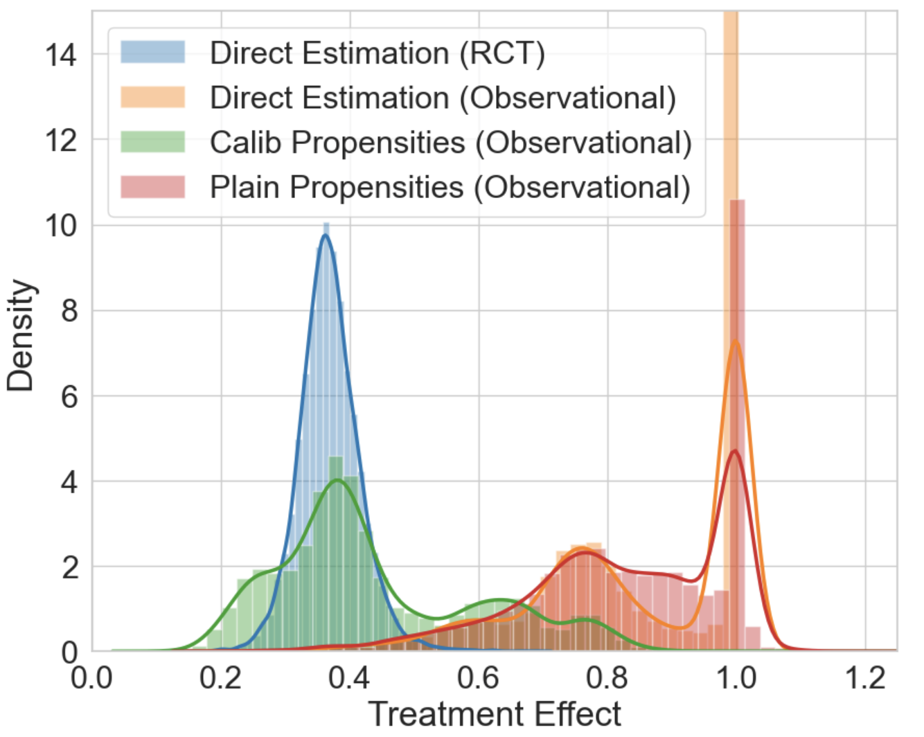
Figure 1: Recalibrating propensity score model reduces the bias in estimating treatment effect from observational data.

Setup.

We use the Inverse-Propensity Treatment Weight (IPTW) and Augmented Inverse Propensity Weight (AIPW) estimators in our experiments. We compare the estimates obtained through calibrated propensities with several baselines including estimators based on uncalibrated propensity scores. We use sigmoid or isotonic regression as the recalibrator and utilize cross-validation splits to generate the calibration dataset. We measure the performance in terms of the absolute error in estimating ATE as $\epsilon_{ATE}=|\hat{\tau}-\tau|,$ where $\tau$ is the true treatment effect and $\hat{\tau}$ is our estimated treatment effect.

Analysis of calibration.

We evaluate the calibration of the propensity score model using expected calibration error (ECE), defined as $\mathbb{E}_{p\sim Q(T=1|X)}[|P(T=1|Q(T=1|X)=p)-p|],$ where $Q(T=1|X)$ models the treatment assignment mechanism $P(T=1|X)$. To compute ECE, we divide the probabilistic output range $[0,1]$ into equal-sized intervals $\{I_{0},I_{1},..,I_{M}\}$ such that we can generate buckets $\{B_{i}\}_{i=1}^{M},$ where $B_{i}=\{(X,T,Y)|Q(T=1|X)\in I_{i}\}$. The estimated ECE is then computed as $\sum_{i=1}^{M}\frac{|B_{i}|}{|\bigcup_{j=1}^{M}B_{j}|}|\text{avg}_{i}(B_{i})-\text{pred}_{i}(B_{i})|,$ where $\text{avg}_{i}(B_{i})=\sum_{j=1}^{|B_{i}|}T_{j}/|B_{i}|$ and $\text{pred}_{i}(B_{i})=\sum_{j=1}^{|B_{i}|}Q(T=1|X_{j})/|B_{i}|$.

5.1 Drug effectiveness study

Table 1: Comparison of different base propensity score models.

Base model	$\varepsilon_{ATE}$(Plain)	$\varepsilon_{ATE}$ (Calib)
Log. Reg	0.479 (0.005)	0.091 (0.022)
MLP	0.455 (0.042)	0.027 (0.031)
SVM	0.485 (0.004)	0.454 (0.013)
Naive Bayes	0.471 (0.003)	0.021 (0.018)

We simulate an observational study of recovery time from disease in response to the administration of a drug [51]. The decision to treat an individual with the drug is dependent on the covariates specified as age, gender, and severity of disease. We use logistic regression as the propensity score model. In Figure 1, we see that weighing using recalibrated propensities allows us to approximate the distribution of individual treatment effect estimates better than uncalibrated propensities. In Figure 2, we compare the histogram of propensity scores before and after calibration. Please refer to Appendix 3 for details on the simulation, models used, and calibration plots.

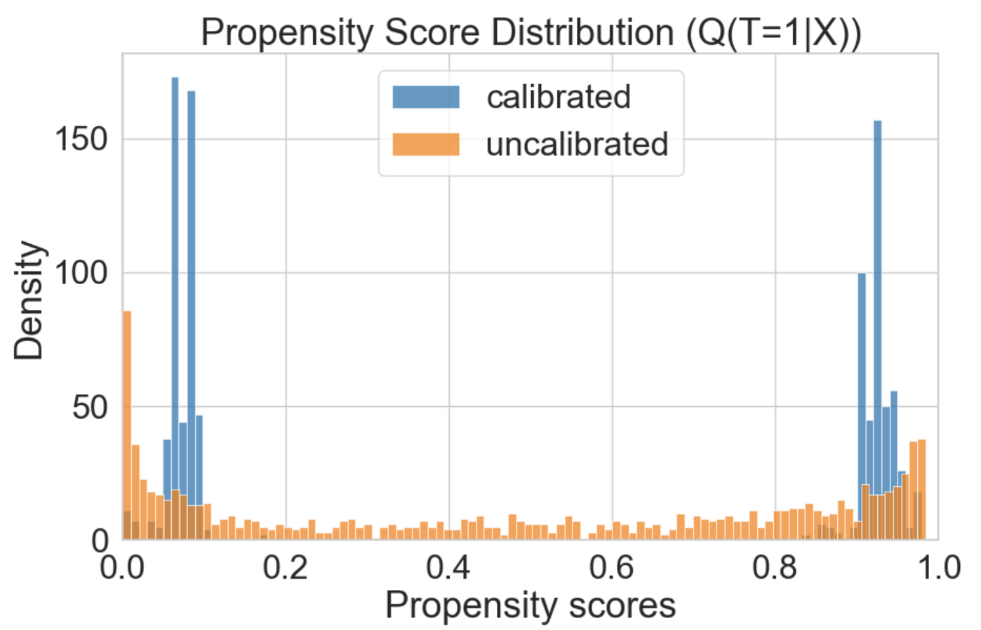
Figure 2: Histogram of propensities pre- and post-calibration. Calibration reduces the occurrence of numerically small scores.

In Table 2, we employ different treatment assignment mechanisms in each simulated observational study, allowing us to compare mechanisms that may or may not be well-specified by a linear model (Appendix 3). We see that calibrated propensities produce lower absolute error in estimating average treatment effect ($\epsilon_{ATE}$) under varying mechanisms. Here, the naive estimation computes the outcomes without weighing the samples with propensities. In Table 1, we also compare a range of base propensity score models for Simulation A and see the benefits of calibration across these setups. Additional details including ECE are in Table 8, Appendix E.

In summary, calibrated propensities approximate the true distribution of individual treatment effects better and reduce the occurrence of numerically low scores. They reduce the error in ATE estimation across different propensity score models and treatment assignment mechanisms. In real-world observational studies, where we don’t know the true treatment assignment mechanism, calibration can be useful to improve the treatment effect estimates from a potentially misspecified model.

Table 2: Recalibrating the output of the propensity score model results in a lower error in estimating causal effects. Reduction in ECE implies that the calibration of the model improves with our technique. Results are averaged over 10 experimental repetitions and braces contain the standard error.

Setting	$\varepsilon_{ATE}$ with	Plain Propensities		Recalibrated Propensities
	naive estimation	$\varepsilon_{ATE}$	ECE	$\varepsilon_{ATE}$	ECE
Simulation A	0.495 (0.002)	0.477 (0.007)	0.033 (0.001)	0.156 (0.027)	0.027 (0.001)
Simulation B	0.222 (0.003)	0.210 (0.002)	0.040 (0.001)	0.193 (0.002)	0.016 (0.001)
Simulation C	0.273 (0.003)	0.153 (0.003)	0.053 (0.001)	0.147 (0.002)	0.025 (0.002)
Simulation D	0.290 (0.004)	0.066 (0.005)	0.118 (0.001)	0.026 (0.004)	0.026 (0.002)

5.2 Unstructured covariates

We simulate a simple observational study following  Louizos et al. [30] and Deshpande et al. [6] such that variables $X,T,Y\sim\mathbb{P}$ are binary and the true ATE is zero. Appendix C contains a detailed description of this simulation. We also introduce an unstructured image covariate $\mathbf{X}$ that represents $X$ as a randomly chosen MNIST image of a zero or one, depending on whether $X=0$ or $X=1$. Specifically, $\mathbb{P}(\mathbf{X}|X=1)\text{ is uniform~{}over MNIST images of `1' }$ and $\mathbb{P}(\mathbf{X}|X=0)\text{ is uniform~{}over MNIST images of `0'}$.

We use a multi-layer perceptron as the propensity score model and recalibrate its output. In Table 3, we compare the IPTW estimates for ATE using binary $X$ and image $\mathbf{X}$ covariates. The ECE is higher for the plain propensity score model trained on image covariates, indicating higher miscalibration. We see that recalibration also improves ATE estimates with high-dimensional, unstructured covariates.

Table 3: Comparison of structured and unstructured covariates.

Setting	$\varepsilon_{ATE}$ with	Plain Propensities		Recalibrated Propensities
	naive estimation	$\varepsilon_{ATE}$	ECE	$\varepsilon_{ATE}$	ECE
Image Covariate	0.187 (0.010)	0.161 (0.046)	0.107 (0.029)	0.095 (0.005)	0.024 (0.003)
Binary Covariate	0.176 (0.019)	0.140 (0.029)	0.052 (0.011)	0.099 (0.008)	0.028 (0.004)

Table 4: GWAS with calibrated propensities. We compare IPTW and AIPW estimates using calibrated propensity scores against standard baselines and a specialized GWAS analysis system (LMM/LIMIX).

Dataset	Spatial	Spatial	Spatial	HGDP	TGP
	($\alpha$=0.1)	($\alpha$=0.3)	($\alpha$=0.5)
Naive	16.23 (0.91)	11.76 (0.84)	9.81 (0.69)	11.82 (0.11)	12.24 (0.71)
PCA	9.60 (0.37)	9.54 (0.41)	9.38 (0.38)	11.69 (0.20)	10.73 (0.38)
FA	9.55 (0.34)	9.53 (0.44)	9.23 (0.30)	11.65 (0.16)	10.59 (0.32)
LMM	10.24 (0.41)	9.58 (0.45)	8.15 (0.40)	10.09 (0.35)	9.44 (0.57)
IPTW (Calib)	8.13 (0.35)	8.69 (0.56)	8.32 (0.34)	10.86 (0.13)	9.57 (0.58)
IPTW (Plain)	12.56 (1.25)	10.22 (0.81)	9.09 (0.48)	11.62 (0.12)	11.76 (0.86)
AIPW (Calib)	8.94 (0.29)	9.00 (0.58)	8.59 (0.39)	11.06 (0.12)	10.32 (0.43)
AIPW (Plain)	13.89 (0.76)	10.46 (0.72)	8.99 (0.51)	11.38 (0.11)	11.56 (0.65)
$\Delta_{ECE}$	0.022 (0.001)	0.016 (0.007)	0.015 (0.001)	0.011 (0.001)	0.022 (0.001)

5.3 Genome-Wide Association Studies

Genome-Wide Association Studies (GWASs) attempt to estimate the treatment effect of genetic mutations (called SNPs) on individual traits (called phenotypes) from observational datasets. Each SNP acts as a treatment. Confounding occurs because of hidden ancestry: individuals with shared ancestry have correlated genes and phenotypes.

The key takeaways can be summarized as follows. First, recalibration enables off-the-shelf IPTW estimators to match or outperform a state-of-the-art GWAS analysis system (LLM/LIMIX; see Tables 4 and 6). Second, our method enables the use of propensity score models that would otherwise be unusable due to the poor quality of their uncertainty estimates (e.g., Naive Bayes; see Table 5). Third, leveraging new types of propensity score models that are fast to train (such as Naive Bayes), improves the speed of GWAS analysis by more than two-fold (see Table 7).

Setup

We simulate the genotypes and phenotypes of individuals following a range of standard models as described in Appendix D. The outcome is simulated as $Y=\beta^{T}G+\alpha^{T}Z+\epsilon,$ where $G$ is the vector of SNPs, $Z$ contains the hidden confounding variables, $\epsilon$ is noise distributed as Gaussian, $\beta$ is the vector of treatment effects corresponding to each SNP and $\alpha$ holds coefficients for the hidden confounding variables. We assume that the aspect of hidden population structure in $Z$ that needs to be controlled for is fully contained in the observed genetic data to ensure ignorability [27]. To estimate the average marginal treatment effect corresponding to each SNP, we iterate successively over the vector of SNPs such that the selected SNP is treatment $T$ and all the remaining SNPs are covariates $X$ for predicting the phenotypic outcome $Y$. The outcome is a vector of estimated treatment effects $\hat{\beta}$ corresponding to the vector of SNPs. We measure $\varepsilon_{ATE}$ as the $l_{2}$ norm of the difference between true and estimated marginal treatment effect vectors.

We use calibrated propensity scores with the IPTW and AIPW estimators to compute these treatment effects. We compare the performance of these estimators with standard methods to perform GWAS, including Principal Components Analysis (PCA) [37; 38], Factor Analysis (FA), and Linear Mixed Models (LMMs) [52; 28], implemented in the popular LIMIX library [29]. Unless mentioned otherwise, 1% of total SNPs are causal and we have 4000 individuals in the dataset.

Table 5: We compare the AIPW estimate using calibrated propensities. Our methods unlock the use of certain propensity score models (e.g., Naive Bayes) which only work after recalibration.

Dataset	Metrics	LR	MLP	Random Forest	Adaboost	NB
Spatial	$\varepsilon_{ATE}$ (plain)	13.886 (0.755)	17.403 (1.070)	12.911 (0.612)	16.234 (0.916)	582.731 (64.514)
($\alpha$=0.1)	$\varepsilon_{ATE}$ (calib)	8.942 (0.287)	14.661 (0.762)	8.706 (0.322)	8.524 (0.297)	8.526 (0.472)
	$\Delta_{ECE}$	0.022 (0.001)	0.072 (0.003)	0.060 (0.001)	0.252 (0.006)	0.281 (0.002)
HGDP	$\varepsilon_{ATE}$ (plain)	11.380 (0.110)	12.358 (0.197)	11.529 (0.107)	11.816 (0.108)	138.086 (5.086)
	$\varepsilon_{ATE}$ (calib)	11.060 (0.120)	11.198 (0.106)	11.299 (0.143)	11.070 (0.123)	11.430 (0.133)
	$\Delta_{ECE}$	0.011 (0.001)	0.069 (0.002)	0.053 (0.001)	0.275 (0.006)	0.206 (0.003)
TGP	$\varepsilon_{ATE}$ (plain)	11.560 (0.650)	11.965 (0.754)	11.677 (0.614)	12.246 (0.713)	87.329 (5.716)
	$\varepsilon_{ATE}$ (calib)	10.320 (0.430)	11.530 (0.633)	10.519 (0.402)	10.244 (0.398)	9.070 (0.316)
	$\Delta_{ECE}$	0.022 (0.001)	0.061 (0.002)	0.070 (0.002)	0.204 (0.007)	0.267 (0.004)

Table 6: Increasing proportion of causal SNPs. Calibrated propensities reduce the bias in treatment effect estimation across all setups and compare favorably against standard GWAS methods.

Method	1% Causal SNPs	2% Causal SNPs	5% Causal SNPs	10% Causal SNPs
Naive	22.408 (5.752)	15.150 (2.213)	23.388 (5.021)	14.846 ( 2.272)
PCA	18.104 (5.378)	13.699 (2.413)	15.837 (3.331)	11.683 (0.983)
FA	18.532 (3.641)	14.166 (2.259)	16.855 (2.764)	11.963 (0.958)
LMM	17.575 (3.408)	13.896 (2.152)	14.681 (3.366)	10.108 (0.827)
IPTW (Calib)	17.237 (3.054)	13.113 (1.775)	14.587 (3.432)	8.625 (0.838)
IPTW (Plain)	19.297 (3.425)	14.372 (1.482)	18.290 (3.788)	11.859 (0.95240)
AIPW (Calib)	17.647 (3.208)	13.382 (1.676)	15.166 (3.597)	9.078 (0.928)
AIPW (Plain)	20.652 (3.286)	13.720 (1.798)	21.321 (4.750)	12.904 (1.990)

In Table 4, we demonstrate the effectiveness of estimators using calibrated propensities on five different GWAS datasets (Appendix D). Here, we have a total of 100 SNPs. In Table 6, we increase the proportion of causal SNPs for the Spatial simulation and continue to see improved performance under calibration. In Table 5, we compare different base models to learn propensity scores and show that calibration improves the performance in each case. We also see that the performance of plain Naive Bayes as the base propensity score model is very poor owing to the simplistic conditional independence assumptions, but calibration improves its performance significantly. In Table 7, we compare the computational throughput of calibrated Naive Bayes as the propensity score model with logistic regression. Here, we have a total of 1000 SNPs. We see that using calibrated Naive Bayes obtains performance competitive with logistic regression at a significantly higher throughput. Please refer to Appendix E for results on additional GWAS datasets.

Table 7: Calibrated Naive Bayes yields lower $\epsilon_{ATE}$ (IPTW) and uses lower computational resources as compared to logistic regression.

Method	$\epsilon_{ATE}$	Tput (SNPs/sec)
LMM	19.908 (3.592)	-
Calibrated NB	18.210 (1.705)	47.6
Plain NB	1455.992 (185.084)	68.6
Calibrated LR	23.618 (3.832)	19.5
Plain LR	27.921 (4.713)	20.1

6 Related work

Isotonic regression [33] and Platt scaling [36] are commonly used to calibrate uncertainties over discrete outputs. This concept has been extended to regression calibration [21], online calibration [19] and structured prediction [20]. Calibrated uncertainties have been used to improve deep reinforcement learning [31; 18], natural language processing [23], Bayesian optimization [5], etc.

Kang and Schafer [17] and  Lenis et al. [26] demonstrate the degradation in treatment effect estimation in response to misspecified treatment and outcome models. Different notions of calibration have been proposed to reduce the bias in treatment effect estimation by optimizing the covariate balancing property [14; 55; 34] and by correcting measurement error [43].

Lin and Zeng [27] rigorously define propensity score-based techniques to correct for confounding in Genome-Wide Association Studies (GWASs).  Zhao et al. [53, 54] propose techniques to balance both genetic and non-genetic covariates using propensity scores. Other techniques to correct for confounding in GWAS include Principal Components Analysis [37], Genomic Control [7], Stratification Scores [8] and Linear Mixed Models [28].

7 Discussion and conclusions

True treatment assignment mechanisms in observational studies are rarely known. Mis-specified propensity score models and outcome models may lead to biased treatment effect estimation [17; 26]. Different parametric and non-parametric models have been proposed to learn propensity scores [32; 13; 15; 25]. We proposed a simple technique to perform post-hoc calibration of the propensity score model. We show that calibration is a necessary condition to obtain accurate treatment effects and calibrated uncertainties improve propensity scoring models. Empirically, we show that our technique reduces bias in estimates across a range of treatment assignment functions and base propensity score models. As compared to calibration by optimizing the covariate balancing property [14], our procedure is simpler and does not require any modification to the training of the base propensity score model. Propensity score models over high-dimensional, unstructured covariates like images, text, and genomic sequences are harder to specify, and we show that we can improve treatment effect estimates for such covariates over a range of base models including the popular logistic regression. We also show that we can calibrate simpler models like Naive Bayes over high-dimensional covariates and obtain higher computational throughput while maintaining competitive performance as measured by the error in treatment effect estimation.

Limitations and future directions

We perform an empirical evaluation for observational studies with binary treatments, but our calibration procedure can be potentially applied to multi-valued and continuous treatments. We leave this as future work. Our GWAS experiments were performed on a range of standard simulation models, but it will be interesting to extend these experiments to include non-genetic covariates, a higher number of SNPs, and real-world genotype matrices. Additionally, the calibration of outcome models is an exciting direction for future work.

Appendix A Estimators for Average Treatment Effects

We expressed ATE as $\tau=\mathbb{E}\bigg{(}\frac{TY}{e(X)}-\frac{(1-T)Y}{1-e(X)}\bigg{)}$. Following  Smith et al. [2020], we can simplify the following term

$$\mathbb{E}\bigg{[}\frac{TY}{e(X)}\bigg{]} =\mathbb{E}[\mathbb{E}\bigg{(}\frac{TY}{e(X)}|T,X\bigg{)}]$$

$$=\mathbb{E}[\bigg{(}\frac{T\mathbb{E}(Y|T,X)}{e(X)}\bigg{)}]$$

$$=\mathbb{E}[\bigg{(}\frac{T\mathbb{E}(Y|T=1,X)}{e(X)}\bigg{)}]$$

$$=\mathbb{E}[\mathbb{E}\bigg{(}\frac{T\mathbb{E}(Y|T=1,X)}{e(X)}|X\bigg{)}]$$

$$=\mathbb{E}[\bigg{(}\frac{\mathbb{E}(Y|T=1,X)P(T=1|X)}{e(X)}\bigg{)}]$$

$$=\mathbb{E}[\mathbb{E}(Y|T=1,X)].$$

Similarly,

$$\mathbb{E}\bigg{[}\frac{(1-T)Y}{1-e(X)}\bigg{]} =\mathbb{E}[\mathbb{E}(Y|T=0,X)].$$

Thus, we can show that ATE is indeed equivalent to $\mathbb{E}\bigg{(}\frac{TY}{e(X)}-\frac{(1-T)Y}{1-e(X)}\bigg{)}$.

Due to sensitivity of the IPTW estimator toward mis-specification of propensity score model,  Robins et al. [2000] propose doubly robust Augmented Inverse Propensity Weighted (AIPW) estimator for ATE. The AIPW estimate is asymptotically unbiased when either the treatment assignment (propensity) model or the outcome model is well-specified.

We define the outcome model as $f(X=x,T=t)$ to approximate the outcome $Y[X=x,T=t]$ as defined in Section 2.

With this, we define the AIPW estimator as

$$\hat{\tau} =\frac{1}{n}\sum_{i=1}^{n}\Bigg{[}f(X_{i},T=1)-f(X_{i},T=0)+\frac{T_{i}(Y_{i}-f(X_{i},T=1))}{e(X_{i})}-\frac{(1-T_{i})(Y_{i}-f(X_{i},T=0))}{1-e(X_{i})}\Bigg{]}$$

Appendix B Drug Effectiveness Simulations

The covariates contain gender ($x_{1}$), age ($x_{2}$) and disease severity ($x_{3}$), while treatment ($t$) corresponds to administration of drug. Outcome ($y$) is the time taken for recovery of patient.

We simulate the covariates as

$$x_{1}\sim\text{Bernoulli}(0.5) x_{2}\sim\text{Gamma}(\alpha=8,\beta=4) x_{3}\sim\text{Beta}(\alpha=3,\beta=1.5).$$

The outcome is simulated as

$$y\sim\text{Poisson}(2+0.5x_{1}+0.03x_{2}+2x_{3}-t).$$

The treatment $t$ is assigned on the basis of the covariates age, gender and severity of disease defined above. The simulations differ in their treatment assignment functions, which are described as follows

1. Simulation A: If $(x_{1}=1)$, set $t=(x_{2}>45)$ else set $t=(x_{3}>0.3).$

2. Simulation B: If $(x_{1}=1)$, set $t=(x_{3}>0.3)$ else set $t=(x_{2}>40).$

3. Simulation C: If $x_{2}>50\text{ AND }x_{3}>0.7$ then set $t=1$ else $t=0$.

4. Simulation D: If $x_{2}>50\text{ XOR }x_{3}>0.7$ then set $t=1$ else $t=0$.

For a linear model predicting treatment given covariates, Simulation C is easier to learn as compared to A, B and D.

Experimental Setup.

We model the outcome using random forests such that the covariates and treatment is taken as input. Logistic regression is used as the propensity score model and the inverse propensity scores are used to weigh each sample while training the outcome model. We use isotonic regression as the recalibrator. The treatment effect is expressed as the ratio $\mathbb{E}(Y(1))/\mathbb{E}(Y(0))$, where $Y(T)$ is the potential outcome $Y$ obtained by setting treatment to $T$. The outcome is time taken by the patient to make full recovery from the disease. We use 10 cross-val splits to generate the recalibration dataset. Isotonic regression is used as the recalibrator.

The experiments were run on a laptop with 2.8GHz quad-core Intel i7 processor.

In Figure 3, we see that the calibration curve of propensity score model gets closer to the diagonal after applying recalibration.

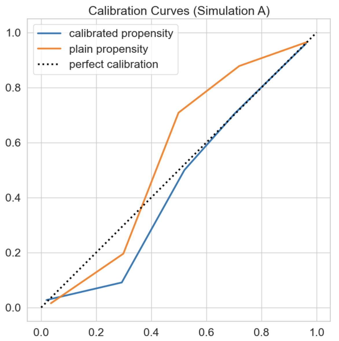
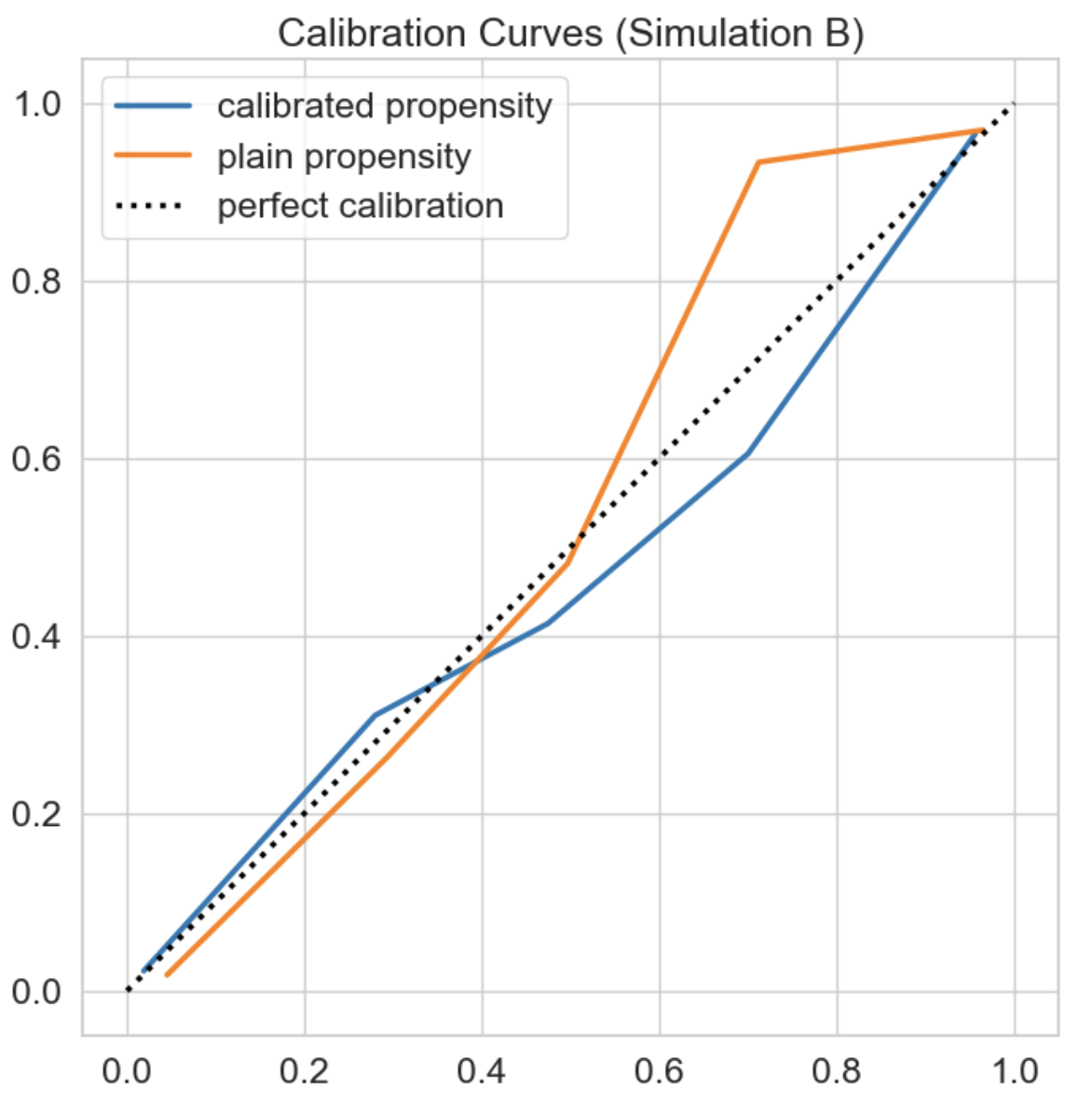
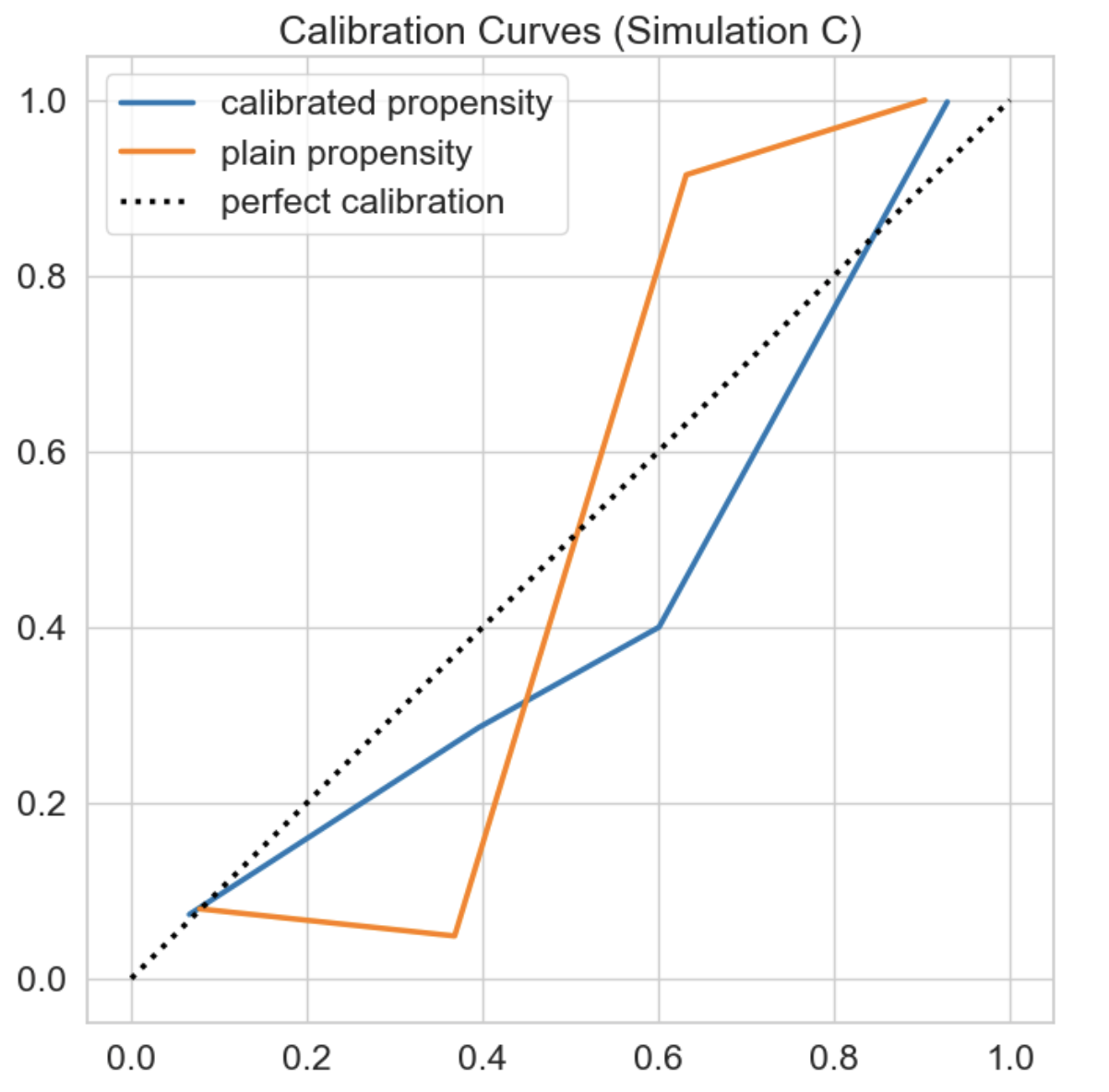
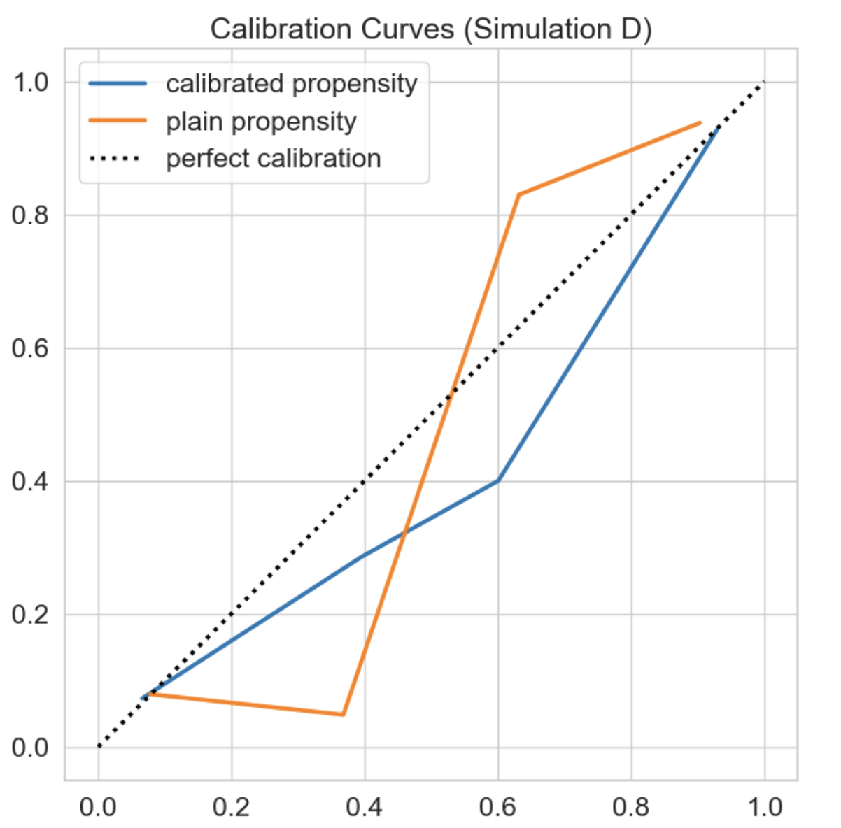
Figure 3: Calibration of propensity score model for Drug Effectiveness Study.

Appendix C Unstructured Covariates Experiment

Following  Louizos et al. [2017], we generate a synthetic observational dataset consisting of binary variables $X,T,Y\sim\mathbb{P}$, such that

$$\mathbb{P}(Z=1)=\mathbb{P}(Z=0)=0.5 \mathbb{P}(X=1|Z=1)=0.3 \mathbb{P}(X=1|Z=0)=0.1$$

$$\mathbb{P}(T=1|Z=1)=0.4 \mathbb{P}(T=1|Z=0)=0.2 Y=T\oplus Z.$$

Louizos et al. [2017] show that the true ATE under this simulation is zero. We would like to note that the presence of hidden confounder $Z$ implies that ignorability is not satisfied in this experiment.

The simulation generation as well as ATE estimation experiments were done on a laptop with 2.8GHz quad-core Intel i7 processor.

Appendix D Simulated GWAS Datasets

We have $N$ individuals and $M$ number of total SNPs for each individual. Thus, we need to simulate a SNP matrix $G\in\{0,1\}^{N\times M}$ and an outcome vector $Y\in\mathbb{R}^{N}$. We also have a matrix of confounding variables $Z\in\mathbb{R}^{N\times D}$ for these $N$ individuals. We do not observe the confounding variables. Following Wang and Blei [2019], we generate the following genotype simulations.

To generate the SNP matrix, we generate an allele frequency matrix $F\in\mathbb{R}^{N\times M}$ such that $F=S\Gamma^{\top},$ where $S\in\mathbb{R}^{N\times D}$ encodes genetic population structure and $\Gamma\in\mathbb{R}^{M\times D}$ maps how structure affects alleles.

Thus, $g_{ij}\sim\text{Binomial}(1,F_{ij})$.

The outcome is modeled as $Y=\beta^{T}G+\alpha^{T}Z+\epsilon,$ where $\beta$ is the vector of treatment effects for each SNP, $\alpha$ is the vector of coefficients corresponding to the hidden confounders in $Z$ and $\epsilon$ is noise distributed independently as a Gaussian.

We simulate a high signal-to-noise ratio while simulating outcomes by replacing $\lambda_{i}=(\alpha^{T}Z)_{i}$ as

$$\lambda_{i}\leftarrow\Bigg{[}\frac{s.d.\{\sum_{j=1}^{m}\beta_{j}g_{ij}\}_{i=1}^{N}}{\sqrt{\nu_{gene}}}\Bigg{]}\Bigg{[}\frac{\sqrt{\nu_{conf}}}{s.d.\{\lambda_{i}\}_{i=1}^{N}}\Bigg{]}\lambda_{i}$$

$$\epsilon_{i}\leftarrow\Bigg{[}\frac{s.d.\{\sum_{j=1}^{m}\beta_{j}g_{ij}\}_{i=1}^{N}}{\sqrt{\nu_{gene}}}\Bigg{]}\Bigg{[}\frac{\sqrt{\nu_{noise}}}{s.d.\{\epsilon_{i}\}_{i=1}^{n}}\Bigg{]}\epsilon_{i},$$

where $\nu_{gene}=0.4,\nu_{conf}=0.4,$ and $\nu_{noise}=0.2$.

Below, we reproduce the simulation details as described by Wang and Blei [2019]. $\Gamma$ and $S$ are simulated in different ways to generate the following datasets.

1. Spatial Dataset: The matrix $\Gamma$ was generated by sampling $\gamma_{ik}\sim 0.9\times\text{Uniform}(0,0.5)$ , for $k=1,2$ and setting $\gamma_{ik}=0.05$. The first two rows of S correspond to coordinates for each individual on the unit square and were set to be independent and identically distributed samples from Beta$(\alpha,\alpha),\alpha=0.1,0.3,0.5,$ while the third row of $S$ was set to be 1, i.e. an intercept. As $\alpha\implies 0$, the individuals are placed closer to the corners of the unit square, while when $\alpha=1$, the individuals are distributed uniformly.

2. Balding-Nichols Model (BN): Each row i of $\Gamma$ has three independent and identically distributed draws taken from the Balding- Nichols model: $\gamma_{ik}\sim BN(p_{i},F_{i})$, where $k\in{1,2,3}$. The pairs $(p_{i},F_{i})$ are computed by randomly selecting a SNP in the HapMap data set, calculating its observed allele frequency and estimating its FST value using the Weir & Cockerham estimator [Weir and Cockerham, 1984]. The columns of $S$ were Multinomial(60/210,60/210,90/210), which reflect the subpopulation proportions in the HapMap dataset.

3. 1000 Genomes Project (TGP) [1000 Genomes Project Consortium et al., 2015]: The matrix $\Gamma$ was generated by sampling $\gamma_{ik}\sim 0.9\text{Uniform}\times(0,0.5)$ , for $k=1,2$ and setting $\gamma_{ik}=0.05$. In order to generate $S$, we compute the first two principal components of the TGP genotype matrix after mean centering each SNP. We then transformed each principal com- ponent to be between (0,1) and set the first two rows of $S$ to be the transformed principal components. The third row of $S$ was set to 1, i.e. an intercept.

4. Humane Genome Diversity Project (HGDP) [Fairley et al., 2019, Bergström et al., 2020]: Same as TGP but generating S with the HGDP genotype matrix.

These simulations and the ATE estimation experiments were all done on a laptop with 2.8GHz quad-core Intel i7 processor.

Appendix E Additional Experimental Results

For the Drug Effectiveness simulations, Table 8 provides additional details on comparing different base propensity score models for Simulation A.

For the GWAS experiments, we provide a complete table of dataset simulations and acomparison against different base propensity models in Table 9 and Table 10 respectively.

Table 8: Calibration reduces the bias in treatment effect estimation across different base models.

Base classifier	Plain Propensities		Recalibrated Propensities
	$\varepsilon_{TE}$	ECE	$\varepsilon_{TE}$	$ECE$
Logistic Regression	0.479 (0.005)	0.029 (0.001)	0.091 (0.022)	0.017 (0.001)
MLP	0.455 (0.042)	0.038 (0.001)	0.027 (0.031)	0.014 (0.001)
SVM	0.485 (0.004)	0.041 (0.001)	0.454 (0.013)	0.018 (0.000)
Naive Bayes	0.471 (0.003)	0.064 (0.000)	0.021 (0.018)	0.003 (0.000)

Table 9: GWAS with calibrated propensities. We compare IPTW and AIPW estimates using calibrated propensity scores against several standard GWAS baselines. $\varepsilon_{ATE}$ is the $l_{2}$ norm of difference between true and estimated marginal treatment effect vector. Under all setups, calibrated propensities improve the treatment effect estimates.

Dataset	Spatial	Spatial	Spatial	Balding	HGDP	TGP
	($\alpha$=0.1)	($\alpha$=0.3)	($\alpha$=0.5)	Nichols
Naive	16.23 (0.91)	11.76 (0.84)	9.81 (0.69)	19.25 (1.17)	11.82 (0.11)	12.24 (0.71)
PCA	9.60 (0.37)	9.54 (0.41)	9.38 (0.38)	14.12 (1.28)	11.69 (0.20)	10.73 (0.38)
FA	9.55 (0.34)	9.53 (0.44)	9.23 (0.30)	12.59 (1.05)	11.65 (0.16)	10.59 (0.32)
LMM	10.24 (0.41)	9.58 (0.45)	8.15 (0.40)	13.13 (1.09)	10.09 (0.35)	9.44 (0.57)
IPTW (Calib)	8.13 (0.35)	8.69 (0.56)	8.32 (0.34)	13.62 (0.68)	10.86 (0.13)	9.57 (0.58)
IPTW (Plain)	12.56 (1.25)	10.22 (0.81)	9.09 (0.48)	14.36 (0.74)	11.62 (0.12)	11.76 (0.86)
AIPW (Calib)	8.94 (0.29)	9.00 (0.58)	8.59 (0.39)	16.81 (1.39)	11.06 (0.12)	10.32 (0.43)
AIPW (Plain)	13.89 (0.76)	10.46 (0.72)	8.99 (0.51)	17.66 (1.33)	11.38 (0.11)	11.56 (0.65)
$\Delta_{ECE}$	0.022 (0.001)	0.016 (0.007)	0.015 (0.001)	0.013 (0.002)	0.011 (0.001)	0.022 (0.001)

Table 10: Comparing propensity score models. We compare the AIPW estimate using calibrated propensities and observe reduction in error across a range of base propensity score models.

Dataset	Metrics	LR	MLP	Random Forest	Adaboost	NB
Spatial	$\varepsilon_{ATE}$ (plain)	13.886 (0.755)	17.403 (1.070)	12.911 (0.612)	16.234 (0.916)	582.731 (64.514)
($\alpha$=0.1)	$\varepsilon_{ATE}$ (calib)	8.942 (0.287)	14.661 (0.762)	8.706 (0.322)	8.524 (0.297)	8.526 (0.472)
	$\Delta_{ECE}$	0.022 (0.001)	0.072 (0.003)	0.060 (0.001)	0.252 (0.006)	0.281 (0.002)
Spatial	$\varepsilon_{ATE}$ (plain)	10.460 (0.720)	12.636 (0.730)	10.578 (0.768)	11.764 (0.839)	400.643 (49.301)
($\alpha$=0.3)	$\varepsilon_{ATE}$ (calib)	9.000 (0.58)	11.550 (0.747)	9.277 (0.532)	8.909 (0.549)	9.121 (0.535)
	$\Delta_{ECE}$	0.016 (0.007)	0.070 (0.003)	0.063 (0.001)	0.244 (0.006)	0.281 (0.002)
Spatial	$\varepsilon_{ATE}$ (plain)	8.990 (0.510)	10.408 (0.694)	9.277 (0.518)	9.814 (0.691)	276.017 (24.183)
($\alpha$=0.5)	$\varepsilon_{ATE}$ (calib)	8.590 (0.390)	9.728 (0.650)	8.687 (0.224)	8.520 (0.286)	8.592 (0.216)
	$\Delta_{ECE}$	0.015 (0.001)	0.070 (0.002)	0.065 (0.001)	0.239 (0.007)	0.269 (0.003)
Balding	$\varepsilon_{ATE}$ (plain)	17.660 (1.330)	18.282 (1.267)	18.419 (1.210)	19.248 (1.169)	95.892 (6.350)
Nichols	$\varepsilon_{ATE}$ (calib)	16.810 (1.390)	17.033 (1.391)	16.611 (1.385)	16.938 (1.367)	16.833 (1.392)
	$\Delta_{ECE}$	0.013 (0.002)	0.041 (0.002)	0.052 (0.002)	0.259 (0.010)	0.261 (0.009)
HGDP	$\varepsilon_{ATE}$ (plain)	11.380 (0.110)	12.358 (0.197)	11.529 (0.107)	11.816 (0.108)	138.086 (5.086)
	$\varepsilon_{ATE}$ (calib)	11.060 (0.120)	11.198 (0.106)	11.299 (0.143)	11.070 (0.123)	11.430 (0.133)
	$\Delta_{ECE}$	0.011 (0.001)	0.069 (0.002)	0.053 (0.001)	0.275 (0.006)	0.206 (0.003)
TGP	$\varepsilon_{ATE}$ (plain)	11.560 (0.650)	11.965 (0.754)	11.677 (0.614)	12.246 (0.713)	87.329 (5.716)
	$\varepsilon_{ATE}$ (calib)	10.320 (0.430)	11.530 (0.633)	10.519 (0.402)	10.244 (0.398)	9.070 (0.316)
	$\Delta_{ECE}$	0.022 (0.001)	0.061 (0.002)	0.070 (0.002)	0.204 (0.007)	0.267 (0.004)

Appendix F Theoretical Analysis

F.1 Notation

As described in Section 2, we are given an observational dataset $\mathcal{D}=\{(x^{(i)},y^{(i)},t^{(i)})\}_{i=1}^{n}$ consisting of $n$ units, each characterized by features $x^{(i)}\in\mathcal{X}\subseteq\mathbb{R}^{d}$, a binary treatment $t^{(i)}\in\{0,1\}$, and a scalar outcome $y^{(i)}\in\mathcal{Y}\subseteq\mathbb{R}$. We assume $\mathcal{D}$ consists of i.i.d. realizations of random variables $X,Y,T\sim P$ from a data distribution $P$. Although we assume binary treatments and scalar outcomes, our approach naturally extends beyond this setting. The feature space $\mathcal{X}$ can be any continuous or discrete set.

F.2 Calibration: a Necessary Condition for Propensity Scoring Models

Theorem F.1.

When $Q(T|X)$ is not calibrated, there exists an outcome function such that an IPTW estimator based on $Q$ yields an incorrect estimate of the true causal effect almost surely.

Example.

Consider a toy binary setting where $\mathcal{X}=\mathcal{T}=\{0,1\},\mathcal{Y}=\{0,1\}^{2}$.

We set $Y=(X\oplus T,\bar{X}\oplus\bar{T})$, $P(T=1|X=0)=p_{0},P(T=1|X=1)=p_{1}$ and $P(X=1)=0.5$ such that $\oplus$ is logical ‘AND’ and $\bar{V}$ denotes logical negation of binary variable $V$. We see that true ATE is $\tau=(0.5,-0.5)$. Let us assume that $Q(T=1|X=0)=q_{0}$ and $Q(T=1|X=1)=q_{1}$. Thus, with IPTW estimator based on $Q$, we estimate $\tau^{\prime}=\mathbb{E}\bigg{(}\frac{TY}{Q(T=1|X)}-\frac{(1-T)Y}{1-Q(T=1|X)}\bigg{)}=(-\frac{0.5(1-p_{0})}{1-q_{0}},\frac{0.5.p_{1}}{q_{1}}).$ The treatment effect $\tau^{\prime}=\tau$ only when $q_{0}=p_{0}$ and $q_{1}=p_{1}$, which is not true if $Q$ is not calibrated. ∎

Proof.

Let $\mathcal{P}$ be a space of valid probability distributions on $\mathcal{Y}$. We would like to prove that $\exists P^{\prime}(Y|X=x,T=t)\in\mathcal{P}$ such that

$$\lim_{n\rightarrow\infty}\text{Probability}(\hat{\tau}_{n}=\tau)=0$$

where

• $\tau$ is the true ATE

• $\hat{\tau}_{n}$ is the ATE estimated using IPTW estimator such that we have $n$ individuals and propensity score model is $Q(T=1|X)$

• The probability is taken over all propensity models $Q(T=1|X)$ such that $\exists q\in[0,1],P(T=1|Q(T=1|X)=q)\neq q$, and all data-generating distributions $P^{\prime}(Y,T,X)=P^{\prime}(Y|X,T).P(T,X)$.

Let $S_{Q}=\{q|\exists X\in\mathcal{X},Q(T=1|X)=q\}$. We partition $\mathcal{X}$ into buckets $\{B_{q}\}_{q\in S_{q}}$ such that $B_{q}=\{X|Q(T=1|X)=q\}$.

Let $\hat{\tau}(Q)=\lim_{n\rightarrow\infty}\tau_{n}$. Thus, for discrete $\mathcal{X},$ we could write

$$\hat{\tau}(Q) =\mathbb{E}_{Y\sim P^{\prime}(.|T,X);T,X\sim P}\left[\left(\frac{TY}{Q(T=1|X)}-\frac{(1-T)Y}{1-Q(T=1|X)}\right)\right]$$

Computing expectation over $$X$$

$$=\sum_{X\in\mathcal{X}}\mathbb{E}_{Y\sim P^{\prime}(.|T,X);T\sim P(.|X)}\left[\left(\frac{TY}{Q(T=1|X)}-\frac{(1-T)Y}{1-Q(T=1|X)}\right)P(X)\right]$$

Computing expectation over $$T$$

$$=\sum_{X\in\mathcal{X}}\mathbb{E}_{Y\sim P^{\prime}(.|X,T=1)}\left[\left(\frac{P(T=1|X)Y}{Q(T=1|X)}\right)P(X)\right]+\sum_{X\in\mathcal{X}}\mathbb{E}_{Y\sim P^{\prime}(.|X,T=0)}\left[\left(-\frac{(1-P(T=1|X))Y}{1-Q(T=1|X)}\right)P(X)\right]$$

$$=\sum_{X\in\mathcal{X}}\left(\mathbb{E}_{Y\sim P^{\prime}(.|X,T=1)}\left[\left(\frac{P(T=1|X)Y}{Q(T=1|X)}\right)\right]-\mathbb{E}_{Y\sim P^{\prime}(.|X,T=0)}\left[\left(\frac{(1-P(T=1|X))Y}{1-Q(T=1|X)}\right)\right]\right)P(X)$$

Expressing the summation over $$X$$ differently

$$=\sum_{q\in S_{Q}}\sum_{X\in{B_{q}}}\left(\mathbb{E}_{Y\sim P^{\prime}(.|X,T=1)}\left[\left(\frac{P(T=1|X)Y}{Q(T=1|X)}\right)\right]-\mathbb{E}_{Y\sim P^{\prime}(.|X,T=0)}\left[\left(\frac{(1-P(T=1|X))Y}{1-Q(T=1|X)}\right)\right]\right)P(X)$$

Since $Q(T=1|X)$ is not calibrated, we know that $\exists q\in[0,1],P(T=1|Q(T=1|X)=q)\neq q.$ Let us pick $q^{\prime}\in S_{Q}$ such that $P(T=1|Q(T=1|X)=q^{\prime})\neq q^{\prime}$.

We could design $P^{\prime}(Y|X,T)=\mathbb{I}(Y=T.\mathbb{I}(X\in B_{q^{\prime}}))$.

Now, we can write

$$\hat{\tau}(Q) =\sum_{q\in S_{Q}}\sum_{X\in{B_{q}}}\left(\mathbb{E}_{Y\sim P^{\prime}(.|X,T=1)}\left[\left(\frac{P(T=1|X)Y}{Q(T=1|X)}\right)\right]-\mathbb{E}_{Y\sim P^{\prime}(.|X,T=0)}\left[\left(\frac{(1-P(T=1|X))Y}{1-Q(T=1|X)}\right)\right]\right)P(X)$$

(Since $$Y=0 T=0 X\notin B_{q^{\prime}}$$ when or )

$$=\sum_{X\in{B_{q^{\prime}}}}\left(\left(\frac{P(T=1|X)P(X)}{Q(T=1|X)}\right)\right)$$

$$=\sum_{X\in{B_{q^{\prime}}}}\left(\left(\frac{P(T=1|X)P(X)}{q^{\prime}}\right)\right)$$

$$=\frac{P(T=1|X\in{B_{q^{\prime}}})P(X\in{B_{q^{\prime}}})}{q^{\prime}}$$

Also, for the above data-generation process,

$$\tau=\hat{\tau}(P) =\sum_{X\in\mathcal{X}}(\mathbb{E}_{Y\sim P^{\prime}(Y|X,do(T=1))}[Y]-\mathbb{E}_{Y\sim P^{\prime}(Y|X,do(T=0))}[Y]).P(X)$$

$$=\sum_{q\in S_{Q}}\sum_{X\in{B_{q}}}(\mathbb{E}_{Y\sim P^{\prime}(Y|X,do(T=1))}[Y]-\mathbb{E}_{Y\sim P^{\prime}(Y|X,do(T=0))}[Y]).P(X)$$

$$=\sum_{X\in{B_{q^{\prime}}}}P(X)$$

$$=P(X\in{B_{q^{\prime}}}))$$

Thus,

$$\lim_{n\rightarrow\infty}\text{Probability}(\tau_{n}=\tau) =P(\hat{\tau}(Q)=\tau)$$

$$=\text{Probability}\left(\frac{P(T=1|X\in{B_{q^{\prime}}})P(X\in{B_{q^{\prime}}})}{q^{\prime}}=P(X\in{B_{q^{\prime}}})\right)$$

$$=\text{Probability}\left(P(T=1|X\in{B_{q^{\prime}}})=q^{\prime}\right)$$

$$=\text{Probability}\left(P(T=1|Q(T=1|X)=q^{\prime})=q^{\prime}\right)$$

$$=0,$$

since we began with the assumption that $P(T=1|Q(T=1|X)=q^{\prime})\neq q^{\prime}$.

Please note that we could have defined a set of outcome functions that produce $Y=0$ for $X\in B_{q^{\prime}}$, thus, potentially letting us compute unbiased treatment effects despite working with a miscalibrated model. However, we want our IPTW estimator to provide unbiased ATE estimates over all possible outcome functions. Here, we can see that IPTW estimator for ATE that uses a miscalibrated propensity score model cannot obtain unbiased treatment effect estimates on all possible outcome functions.

∎

F.3 Calibrated Uncertainties Improve Propensity Scoring Models

We define the true ATE as

$$\tau =\mathbb{E}_{y\sim P(Y=y|do(T=1))}[y]-\mathbb{E}_{y\sim P(Y=y|do(T=0))}[y]$$

$$=\sum_{y}y(\sum_{X}P(Y=y|X,do(T=1))P(X)-\sum_{X}P(Y=y|X,do(T=0))P(X))$$

$$=\sum_{y}y(\sum_{X}P(Y=y|X,T=1)P(X)-\sum_{X}P(Y=y|X,T=0)P(X))$$

Next, recall that the finite-sample Inverse Propensity of Treatment Weight (IPTW) estimator with a model $Q(T=1|X)$ of $P(T=1|X)$ produces an estimate $\hat{\tau}_{n}(Q)$ of the ATE, which is computed as

$$\hat{\tau}_{n}(Q)=\frac{1}{n}\sum_{i=1}^{n}\bigg{(}\frac{t^{(i)}y^{(i)}}{Q(T=1|x^{(i)})}-\frac{(1-t^{(i)})y^{(i)}}{1-Q(T=1|x^{(i)})}\bigg{)}.$$

We define $\tau(Q)$ as the limit $lim_{n\rightarrow\infty}\hat{\tau}_{n}(Q)$ when the amount of data goes to infinity. Notice that we can write

$$\lim_{n\rightarrow\infty}(\hat{\tau}_{n}(Q))=\hat{\tau}(Q)=\sum_{y}y[\pi_{y,1}(Q)-\pi_{y,0}(Q)]$$

where

$$\pi_{y,t}(Q)=P(T=t)\sum_{X}P(Y=y|X,T=t)\frac{P(X|T=t)}{Q(T=t|X)}=\sum_{X}P(Y=y|X,T=t)\frac{P(T=t|X)}{Q(T=t|X)}{P(X)}$$

We have a multiplicative term $P(T=t)$ in the above expression since we are dividing by $n$ in the finite-sample formula as opposed to $n_{t}$ (the number of samples with treatment $t$). In other words, in order for the finite-sample formula to be a valid Monte Carlo estimator with samples coming from $P(X|T=t)$, there needs to be an "effective adjustment factor" of $n_{t}/n$ (such that $(n_{t}/n)\cdot(1/n_{t})=(1/n)$), and this term is $P(T=t)$ in the limit of infinite data.

Clearly, if $Q=P$ we have $\hat{\tau}(Q)=\hat{\tau}(P)=\tau$. If not, we can consider the error

$$E=|(\hat{\tau}(P)-\hat{\tau}(Q))|.$$

F.3.1 Bounding the Error of Causal Effect Estimation Using Proper Losses

We can form a bound on $E$ as

$$E =|[\hat{\tau}(P)-\hat{\tau}(Q)]|$$

$$=\left|\sum_{y}y[(\pi_{y,1}(P)-\pi_{y,0}(P))-(\pi_{y,1}(Q)-\pi_{y,0}(Q))]\right|$$

$$\leq\sum_{t}\left|\sum_{y}y[(\pi_{y,t}(P)-\pi_{y,t}(Q)]\right|$$

$$\leq\sum_{t}\sum_{y}[|y||\pi_{y,t}(P)-\pi_{y,t}(Q)|]$$

$$=\sum_{t}\sum_{y}|y|[\left|\sum_{X}P(Y=y|X,T=t){P(X)}\left(1-\frac{P(T=t|X)}{Q(T=t|X)}\right)\right|]$$

$$\leq\sum_{t}\sum_{y}|y|[\sum_{X}P(Y=y|X,T=t){P(X)}\left|1-\frac{P(T=t|X)}{Q(T=t|X)}\right|]$$

$$=\sum_{t}\sum_{y}|y|.[\sum_{X}P(Y=y|X,T=t)P(X)\ell_{X}(P,Q)^{1/2}] \text{where }\ell_{X}(P,Q)=\left(1-\frac{P(T=t|X)}{Q(T=t|X)}\right)^{2}$$

$$=\sum_{t}\sum_{y}|y|.\mathbb{E}_{X\sim R_{y,t}}[\ell_{X}(P,Q)^{1/2}]$$

where $R_{t,y}\propto P(Y=y|X,T=t)P(X)$ (i.e. $R_{t,y}\sim k.P(Y=y|X,T=t)P(X)$, $k$ is constant) and $\ell_{X}(P,Q)$ is a type of expected Chi-Squared divergence between $P,Q$. It is a type of proper score. Thus when $P=Q$, we get zero error, and otherwise we get a bound.

In the above derivation, we see that the expected error $|\pi_{y,t}(P)-\pi_{y,t}(Q)|$ induced by an IPTW estimator with propensity score model $Q$ is bounded as

$$|\pi_{y,t}(P)-\pi_{y,t}(Q)|\leq\mathbb{E}_{X\sim R_{y,t}}[\ell_{\chi}(P,Q)^{\frac{1}{2}}].$$

F.3.2 Calibration Reduces Variance of Inverse Probability Estimators

Theorem F.2.

Let $P$ be the data distribution, and suppose that $1-\delta>P(T|X)>\delta$ for all $T,X$ and let $Q$ be a calibrated model relative to $P$. Then $1-\delta>Q(T|X)>\delta$ for all $T,X$ as well.

Proof.

Suppose $Q(T=1|x)=q$ for some $x$ and $q<\delta$. Since $Q$ is calibrated, we have $P(T=1|Q(T=1|X)=q)=q<\delta$.

However $P(T=1|x)>\delta$ for every $x$. Hence, $P(T=1|X\in A)>\delta$, for all sets $A\subseteq\mathcal{X}$. This implies that $P(T=1|Q(T=1|X)=q)>\delta$ for all $q\in[0,1].$

Thus, we have a contradiction. ∎

F.3.3 Calibration Improves the Accuracy of Causal Effect Estimation

Theorem F.3.

The error of an IPTW estimator with propensity model $Q$ tends to zero as $n\to\infty$ if:

1. Separability holds, i.e., $\forall X_{1},X_{2}\in\mathcal{X},P(T|X_{1})\neq P(T|X_{2})\implies Q(T|X_{1})\neq Q(T|X_{2})$

2. The model $Q$ is calibrated, i.e., $\forall q\in(0,1),P(T=1|Q(T=1|X)=q)=q$

Proof.

We prove this for discrete inputs at first and then prove it for continuous inputs.

Discrete Input Space.

If our input space $\mathcal{X}$ is discrete, then the number of distinct values that $Q(T=1|X)$ can take is countable. Let us assume that $Q(T=1|X)$ takes values $\{q_{i}\}_{i=1}^{M}$. Thus, we can partition $\mathcal{X}$ into buckets $\{B_{i}\}_{i=1}^{M}$ such that $B_{i}=\{X|Q(T=1|X)=q_{i}\}$. Due to separability, we have $\forall X_{1},X_{2}\in\mathcal{X},Q(T|X_{1})=Q(T|X_{2})\implies P(T|X_{1})=P(T|X_{2})$. Thus, we have $\forall i,\forall X_{1},X_{2}\in B_{i},Q(T=1|X_{1})=Q(T=1|X_{2}),$ and $P(T=1|X_{1})=P(T=1|X_{2}).$

Let us assume that for each bucket $B_{i}$, our true propensity $P(T=1|X)$ is $p_{i}$, i.e, if $X\in B_{i}$ then $Q(T=1|X)=q_{i}$ and $P(T=1|X)=p_{i}$.

Assuming positivity, $0<p_{i}<1$.

Now, for all $i$, we can write

$$P(T=1|Q(T=1|X)=q_{i}) =P(T=1|X\in B_{i})$$

$$=p_{i}.$$

If $Q$ is calibrated, then by definition $p_{i}=q_{i}$.

Now, we can write the expression for ATE $\tau$ as

$${\tau}=\hat{\tau}(P) =\mathbb{E}_{Y,T,X}[\frac{TY}{P(T=1|X)}-\frac{(1-T)Y}{(1-P(T=1|X))}]$$

$$=\sum_{i=1}^{N}P(X\in B_{i})\mathbb{E}_{Y,T}\left(\frac{TY}{p_{i}}-\frac{(1-T)Y}{(1-p_{i})}\right)$$

Using our propensity score model $Q(T=1|X)$, we estimate $\hat{\tau}$ as

$$\hat{\tau}(Q) =\mathbb{E}_{Y,T,X}[\frac{TY}{Q(T=1|X)}-\frac{(1-T)Y}{(1-Q(T=1|X))}]$$

$$=\sum_{i=1}^{N}P(X\in B_{i})\mathbb{E}_{Y,T}\left(\frac{TY}{q_{i}}-\frac{(1-T)Y}{(1-q_{i})}\right)$$

If our model $Q$ is calibrated, then $p_{i}=q_{i}$. Hence, $0<q_{i}<1$ and $\hat{\tau}$ is well-defined. Also, $\tau=\hat{\tau}(P)=\hat{\tau}(Q)$.

When our observational data contains $n$ units, the IPTW estimator based on model $Q(T=1|X)$ is $\hat{\tau}_{n}=\frac{1}{n}\sum_{i=0}^{n}\left(\frac{T^{(i)}Y^{(i)}}{Q(T=1|X^{(i)})}-\frac{(1-T^{(i)})Y^{(i)}}{1-Q(T=1|X^{(i)})}\right).$

Hence, $\lim_{n\rightarrow\infty}\hat{\tau}_{n}=\hat{\tau}(Q)=\hat{\tau}(P)=\tau.$

Continuous Input Space.

When $X$ is continuous, the number of buckets can be uncountable. The buckets can now be formed as $B_{q}=\{X|Q(T=1|X)=q\},\forall q\in[0,1]$. It is easy to see that $\{B_{q}\}_{q\in[0,1]}$ partitions $\mathcal{X}$. Note that $B_{q}$ can be empty if there exists no $X$ such that $Q(T=1|X)=q$.

Due to separability, $\forall X_{1},X_{2}\in\mathcal{X},Q(T|X_{1})=Q(T|X_{2})\implies P(T|X_{1})=P(T|X_{2})$. Thus, for all $q$, $P(T=1|X)$ takes on a unique value for all $X\in B_{q}$, i.e., $\forall q\in[0,1],P(T=1|X\in B_{q})=f(q),$ where function $f:[0,1]\rightarrow[0,1]$.

Hence, we can write

$$\forall q\in[0,1],P(T=1|Q(T=1|X)=q) =P(T=1|X\in B_{q})$$

$$=f(q).$$

When model $Q(T=1|X)$ is calibrated by our definition, then $\forall q\in[0,1],q=f(q).$

Therefore, $\forall q\in[0,1],Q(T=1|X\in B_{q})=q=f(q)=P(T=1|X\in B_{q})$.

Since $\{B_{q}\}_{q\in[0,1]}$ partitions $\mathcal{X}$, we have $\forall X\in\mathcal{X},P(T=1|X)=Q(T=1|X)$. Thus, $\hat{\tau}(P)=\hat{\tau}(Q)$.

∎

F.4 Algorithms for Calibrated Propensity Scoring

F.4.1 Asymptotic Calibration Guarantee

Theorem F.4.

The model $R\circ Q$ is asymptotically calibrated and the calibration error $\mathbb{E}[L_{c}(R\circ Q,S)]<\delta(m)$ for $\delta(m)=o(m^{-k}),k>0$ w.h.p.

Proof.

Any proper loss can be decomposed as: proper loss = calibration - sharpness + irreducible term [Guo et al., 2017]. The calibration term consists of the error $\mathbb{E}[L_{c}(R\circ Q,S)]$. The sharpness and irreducible term can be represented as the refinement term $\mathbb{E}(L_{r}(S))$. Table 11 provides examples of some proper loss functions and the respective decompositions. The rest of our proof uses the techniques of Kuleshov and Deshpande [2022] in the context of propensity scores.

Kull and Flach [2015] show that the refinement term can be further divided as $\mathbb{E}(L_{r}(S))=\mathbb{E}(L_{g}(S,B\circ Q))+\mathbb{E}(L(B\circ Q,T)).$ Here, $B$ is the Bayes optimal recalibrator $P(T=1|Q(T=1|X))$ and $S$ is $P(T=1|R\circ Q).$

Recall that if we solve the Task 4.1, we have for $\delta(m)=o(1)$

$$\mathbb{E}(L(B\circ Q,T)) \leq\mathbb{E}(L(R\circ Q,T))\leq\mathbb{E}(L(B\circ Q,T))+\delta(m)$$

$$\text{Using \cite[citet]{\@@bibref{Authors Phrase1YearPhrase2}{gneiting2007probabilistic}{\@@citephrase{[}}{\@@citephrase{]}}}}, \mathbb{E}(L(R\circ Q,T))$$  Kull and Flach [2015] we decompose

$$\implies\mathbb{E}(L(B\circ Q,T)) \leq\mathbb{E}(L_{c}(R\circ Q,S))+\mathbb{E}(L_{g}(S,B\circ Q))+\mathbb{E}(L(B\circ Q,T))\leq\mathbb{E}(L(B\circ Q,T))+\delta(m)$$

$$\implies\mathbb{E}(L_{c}(R\circ Q,S)) +\mathbb{E}(L_{g}(S,B\circ Q))\leq\delta(m)$$

$$\implies\mathbb{E}(L_{c}(R\circ Q,S)) \leq\delta(m)$$

Proper Score	Loss	Calibration	Refinement
	$L(F,G)$	$L_{c}(F,S)$	$L_{r}(S)$
Logarithmic	$\mathbb{E}_{y\sim G}$ $\log f(y)$	$\text{KL}(s||f)$	$H(s)$
CRPS	$\mathbb{E}_{y\sim G}$ $(F(y)-G(y))^{2}$	$\int^{\infty}_{-\infty}(F(y)-S(y))^{2}$dy	$\int^{\infty}_{-\infty}S(y)(1-S(y))dy$
Quantile	$\mathbb{E}^{\tau\in U[0,1]}_{y\sim G}\rho_{\tau}(y-F^{-1}(\tau))$	$\int_{0}^{1}\int^{F^{-1}(\tau)}_{S^{-1}(\tau)}(S(y)-\tau)dyd\tau$	$\mathbb{E}^{\tau\in U[0,1]}_{y\sim S}\rho_{\tau}(y-S^{-1}(\tau))$

Table 11: Proper loss functions. A proper loss is a function $L(F,G)$ over a forecast $F$ targeting a variable $y\in\mathcal{Y}$ whose true distribution is $G$ and for which $S(F,G)\geq S(G,G)$ for all $F$. Each $L(F,G)$ decomposes into the sum of a calibration loss term $L_{c}(F,S)$ (also known as reliability) and a refinement loss term $L_{r}(S)$ (which itself decomposes into sharpness and an uncertainty term). Here, $S(y)$ denotes the cumulative distribution function of the conditional distribution $\mathbb{P}(Y=y\mid F_{X}=F)$ of $Y$ given a forecast $F$, and $s(y),f(y)$ are the probability density functions of $S$ and $F$, respectively. We give three examples of proper losses: the log-loss, the continuous ranked probability score (CRPS), and the quantile loss.

Thus, solving Task 4.1 allows us to obtain asymptotically calibrated $R\circ Q$ such that the calibration error is bounded as $\mathbb{E}[L_{c}(R\circ Q,S)]<\delta(m)$.

∎

F.4.2 No-Regret Calibration

Theorem F.5.

The recalibrated model has asymptotically vanishing regret relative to the base model: $\mathbb{E}[L(R\circ Q,T)]\leq\mathbb{E}[L(Q,T)]+\delta,$ where $\delta>0,\delta=o(m^{-k}),k>0$.

Proof.

Solving Task 4.1 implies $\mathbb{E}[L(R\circ Q,T)]\leq\mathbb{E}[L(B\circ Q,T)]+\delta\leq\mathbb{E}[L(Q,T)]+\delta$. The first inequality comes from definition of Task 4.1 and the second inequality holds because a Bayes-optimal $B$ has lower loss than an identity mapping [Kuleshov and Deshpande, 2022].

∎

References

- 1000 Genomes Project Consortium et al. [2015] 1000 Genomes Project Consortium, Adam Auton, Lisa D Brooks, Richard M Durbin, Erik P Garrison, Hyun Min Kang, Jan O Korbel, Jonathan L Marchini, Shane McCarthy, Gil A McVean, and Gonçalo R Abecasis. A global reference for human genetic variation. Nature, 526(7571):68–74, October 2015.
- Angelopoulos and Bates [2021] Anastasios N. Angelopoulos and Stephen Bates. A gentle introduction to conformal prediction and distribution-free uncertainty quantification, 2021. URL https://arxiv.org/abs/2107.07511.
- Bergström et al. [2020] Anders Bergström, Shane A. McCarthy, Ruoyun Hui, Mohamed A. Almarri, Qasim Ayub, Petr Danecek, Yuan Chen, Sabine Felkel, Pille Hallast, Jack Kamm, Hélène Blanché, Jean-François Deleuze, Howard Cann, Swapan Mallick, David Reich, Manjinder S. Sandhu, Pontus Skoglund, Aylwyn Scally, Yali Xue, Richard Durbin, and Chris Tyler-Smith. Insights into human genetic variation and population history from 929 diverse genomes. Science, 367(6484):eaay5012, 2020. doi: 10.1126/science.aay5012. URL https://www.science.org/doi/abs/10.1126/science.aay5012.
- D’Agostino [1998] Ralph B D’Agostino. Propensity score methods for bias reduction in the comparison of a treatment to a non-randomized control group. Stat. Med., 17(19):2265–2281, October 1998.
- Deshpande and Kuleshov [2023] Shachi Deshpande and Volodymyr Kuleshov. Calibrated uncertainty estimation improves bayesian optimization, 2023.
- Deshpande et al. [2022] Shachi Deshpande, Kaiwen Wang, Dhruv Sreenivas, Zheng Li, and Volodymyr Kuleshov. Deep multi-modal structural equations for causal effect estimation with unstructured proxies. In S. Koyejo, S. Mohamed, A. Agarwal, D. Belgrave, K. Cho, and A. Oh, editors, Advances in Neural Information Processing Systems, volume 35, pages 10931–10944. Curran Associates, Inc., 2022. URL https://proceedings.neurips.cc/paper_files/paper/2022/file/46e654963ca9f2b9ff05d1bbfce2420c-Paper-Conference.pdf.
- Devlin and Roeder [1999] B Devlin and K Roeder. Genomic control for association studies. Biometrics, 55(4):997–1004, December 1999.
- Epstein et al. [2007] Michael P Epstein, Andrew S Allen, and Glen A Satten. A simple and improved correction for population stratification in case-control studies. Am. J. Hum. Genet., 80(5):921–930, May 2007.
- Fairley et al. [2019] Susan Fairley, Ernesto Lowy-Gallego, Emily Perry, and Paul Flicek. The International Genome Sample Resource (IGSR) collection of open human genomic variation resources. Nucleic Acids Research, 48(D1):D941–D947, 10 2019. ISSN 0305-1048. doi: 10.1093/nar/gkz836. URL https://doi.org/10.1093/nar/gkz836.
- Gneiting et al. [2007] T. Gneiting, F. Balabdaoui, and A. E. Raftery. Probabilistic forecasts, calibration and sharpness. Journal of the Royal Statistical Society: Series B (Statistical Methodology), 69(2):243–268, 2007.
- Greenland et al. [1999] Sander Greenland, Judea Pearl, and James M. Robins. Confounding and Collapsibility in Causal Inference. Statistical Science, 14(1):29 – 46, 1999. doi: 10.1214/ss/1009211805. URL https://doi.org/10.1214/ss/1009211805.
- Guo et al. [2017] Chuan Guo, Geoff Pleiss, Yu Sun, and Kilian Q. Weinberger. On calibration of modern neural networks, 2017.
- Hirano et al. [2003] Keisuke Hirano, Guido W. Imbens, and Geert Ridder. Efficient estimation of average treatment effects using the estimated propensity score. Econometrica, 71(4):1161–1189, 2003. ISSN 0012-9682. doi: 10.1111/1468-0262.00442.
- Imai and Ratkovic [2014] Kosuke Imai and Marc Ratkovic. Covariate balancing propensity score. J. R. Stat. Soc. Series B Stat. Methodol., 76(1):243–263, January 2014.
- Imbens [2004] Guido W Imbens. Nonparametric estimation of average treatment effects under exogeneity: A review. Rev. Econ. Stat., 86(1):4–29, February 2004.
- Kallus [2020] Nathan Kallus. Deepmatch: Balancing deep covariate representations for causal inference using adversarial training. In International Conference on Machine Learning, pages 5067–5077. PMLR, 2020.
- Kang and Schafer [2007] Joseph D. Y. Kang and Joseph L. Schafer. Demystifying double robustness: A comparison of alternative strategies for estimating a population mean from incomplete data. Statistical Science, 22(4), nov 2007. doi: 10.1214/07-sts227. URL https://doi.org/10.1214%2F07-sts227.
- Kuleshov and Deshpande [2022] Volodymyr Kuleshov and Shachi Deshpande. Calibrated and sharp uncertainties in deep learning via density estimation. In Kamalika Chaudhuri, Stefanie Jegelka, Le Song, Csaba Szepesvari, Gang Niu, and Sivan Sabato, editors, Proceedings of the 39th International Conference on Machine Learning, volume 162 of Proceedings of Machine Learning Research, pages 11683–11693. PMLR, 17–23 Jul 2022. URL https://proceedings.mlr.press/v162/kuleshov22a.html.
- Kuleshov and Ermon [2017] Volodymyr Kuleshov and Stefano Ermon. Estimating uncertainty online against an adversary. In AAAI, pages 2110–2116, 2017.
- Kuleshov and Liang [2015] Volodymyr Kuleshov and Percy S Liang. Calibrated structured prediction. In C. Cortes, N. Lawrence, D. Lee, M. Sugiyama, and R. Garnett, editors, Advances in Neural Information Processing Systems, volume 28. Curran Associates, Inc., 2015. URL https://proceedings.neurips.cc/paper/2015/file/52d2752b150f9c35ccb6869cbf074e48-Paper.pdf.
- Kuleshov et al. [2018] Volodymyr Kuleshov, Nathan Fenner, and Stefano Ermon. Accurate uncertainties for deep learning using calibrated regression, 2018.
- Kull and Flach [2015] Meelis Kull and Peter Flach. Novel decompositions of proper scoring rules for classification: Score adjustment as precursor to calibration. In Annalisa Appice, Pedro Pereira Rodrigues, Vítor Santos Costa, Carlos Soares, João Gama, and Alípio Jorge, editors, Machine Learning and Knowledge Discovery in Databases, pages 68–85, Cham, 2015. Springer International Publishing. ISBN 978-3-319-23528-8.
- Kumar and Sarawagi [2019] Aviral Kumar and Sunita Sarawagi. Calibration of encoder decoder models for neural machine translation, 2019.
- Lanza et al. [2013] Stephanie T Lanza, Julia E Moore, and Nicole M Butera. Drawing causal inferences using propensity scores: a practical guide for community psychologists. Am. J. Community Psychol., 52(3-4):380–392, December 2013.
- Lee et al. [2010] Brian K Lee, Justin Lessler, and Elizabeth A Stuart. Improving propensity score weighting using machine learning. Stat. Med., 29(3):337–346, February 2010.
- Lenis et al. [2018] David Lenis, Benjamin Ackerman, and Elizabeth A Stuart. Measuring model misspecification: Application to propensity score methods with complex survey data. Comput. Stat. Data Anal., 128:48–57, December 2018.
- Lin and Zeng [2011] D Y Lin and D Zeng. Correcting for population stratification in genomewide association studies. J. Am. Stat. Assoc., 106(495):997–1008, September 2011.
- Lippert et al. [2011] Christoph Lippert, Jennifer Listgarten, Ying Liu, Carl M Kadie, Robert I Davidson, and David Heckerman. Fast linear mixed models for genome-wide association studies. Nature methods, 8(10):833–835, 2011.
- Lippert et al. [2014] Christoph Lippert, Francesco Paolo Casale, Barbara Rakitsch, and Oliver Stegle. Limix: genetic analysis of multiple traits. BioRxiv, 2014.
- Louizos et al. [2017] Christos Louizos, Uri Shalit, Joris Mooij, David Sontag, Richard Zemel, and Max Welling. Causal effect inference with deep latent-variable models. arXiv preprint arXiv:1705.08821, 2017.
- Malik et al. [2019] Ali Malik, Volodymyr Kuleshov, Jiaming Song, Danny Nemer, Harlan Seymour, and Stefano Ermon. Calibrated model-based deep reinforcement learning, 2019.
- McCaffrey et al. [2004] Daniel F McCaffrey, Greg Ridgeway, and Andrew R Morral. Propensity score estimation with boosted regression for evaluating causal effects in observational studies. Psychol. Methods, 9(4):403–425, December 2004.
- Niculescu-Mizil and Caruana [2005] Alexandru Niculescu-Mizil and Rich Caruana. Predicting good probabilities with supervised learning. In Proceedings of the 22nd International Conference on Machine Learning, ICML ’05, page 625–632, New York, NY, USA, 2005. Association for Computing Machinery. ISBN 1595931805. doi: 10.1145/1102351.1102430. URL https://doi.org/10.1145/1102351.1102430.
- Ning et al. [2018] Yang Ning, Sida Peng, and Kosuke Imai. Robust estimation of causal effects via high-dimensional covariate balancing propensity score, 2018.
- Pearl et al. [2000] Judea Pearl et al. Models, reasoning and inference. Cambridge, UK: CambridgeUniversityPress, 19, 2000.
- Platt [1999] John C. Platt. Probabilistic outputs for support vector machines and comparisons to regularized likelihood methods. In ADVANCES IN LARGE MARGIN CLASSIFIERS, pages 61–74. MIT Press, 1999.
- Price et al. [2006] AL Price, NJ Patterson, RM Plenge, ME Weinblatt, Shadick NA, and Reich D. Principal components analysis corrects for stratification in genome-wide association studies., 2006.
- Price et al. [2010] Alkes L Price, Noah A Zaitlen, David Reich, and Nick Patterson. New approaches to population stratification in genome-wide association studies. Nature reviews genetics, 11(7):459–463, 2010.
- Robins et al. [2000] James M Robins, Andrea Rotnitzky, and Mark van der Laan. On profile likelihood: Comment. J. Am. Stat. Assoc., 95(450):477, June 2000.
- Rosenbaum and Rubin [1983] Paul R Rosenbaum and Donald B Rubin. The central role of the propensity score in observational studies for causal effects. Biometrika, 70(1):41, April 1983.
- Shafer and Vovk [2007] Glenn Shafer and Vladimir Vovk. A tutorial on conformal prediction, 2007.
- Smith et al. [2020] Matthew J. Smith, Camille Maringe, Bernard Rachet, Mohammad A. Mansournia, Paul N. Zivich, Stephen R. Cole, and Miguel Angel Luque-Fernandez. Tutorial: Introduction to computational causal inference using reproducible stata, r and python code, 2020.
- Stürmer et al. [2007] Til Stürmer, Sebastian Schneeweiss, Kenneth J Rothman, Jerry Avorn, and Robert J Glynn. Performance of propensity score calibration–a simulation study. Am. J. Epidemiol., 165(10):1110–1118, May 2007.
- Tan [2017] Zhiqiang Tan. Regularized calibrated estimation of propensity scores with model misspecification and high-dimensional data, 2017.
- VanderWeele [2006] Tyler VanderWeele. The use of propensity score methods in psychiatric research. Int. J. Methods Psychiatr. Res., 15(2):95–103, June 2006.
- Veitch et al. [2019] Victor Veitch, Yixin Wang, and David M. Blei. Using embeddings to correct for unobserved confounding in networks, 2019.
- Vovk et al. [2005] Vladimir Vovk, Akimichi Takemura, and Glenn Shafer. Defensive forecasting. In Proceedings of the Tenth International Workshop on Artificial Intelligence and Statistics, AISTATS 2005, Bridgetown, Barbados, January 6-8, 2005, 2005. URL http://www.gatsby.ucl.ac.uk/aistats/fullpapers/224.pdf.
- Wang and Blei [2019] Yixin Wang and David M Blei. The blessings of multiple causes. Journal of the American Statistical Association, 114(528):1574–1596, 2019.
- Wasserman [2004] Larry Wasserman. Nonparametric Curve Estimation, pages 303–326. Springer New York, New York, NY, 2004. ISBN 978-0-387-21736-9. doi: 10.1007/978-0-387-21736-9_20. URL https://doi.org/10.1007/978-0-387-21736-9_20.
- Weir and Cockerham [1984] Bruce S Weir and C Clark Cockerham. Estimating f-statistics for the analysis of population structure. evolution, pages 1358–1370, 1984.
- [51] Florian Wilhelm. Causal inference and propensity score methods. https://florianwilhelm.info/2017/04/causal_inference_propensity_score/. URL https://florianwilhelm.info/2017/04/causal_inference_propensity_score/.
- Yu et al. [2006] Jianming Yu, Gael Pressoir, William H Briggs, Irie Vroh Bi, Masanori Yamasaki, John F Doebley, Michael D McMullen, Brandon S Gaut, Dahlia M Nielsen, James B Holland, et al. A unified mixed-model method for association mapping that accounts for multiple levels of relatedness. Nature genetics, 38(2):203–208, 2006.
- Zhao et al. [2009] Huaqing Zhao, Timothy R Rebbeck, and Nandita Mitra. A propensity score approach to correction for bias due to population stratification using genetic and non-genetic factors. Genet. Epidemiol., 33(8):679–690, December 2009.
- Zhao et al. [2012] Huaqing Zhao, Timothy R Rebbeck, and Nandita Mitra. Analyzing genetic association studies with an extended propensity score approach. Stat. Appl. Genet. Mol. Biol., 11(5), October 2012.
- Zhao [2017] Qingyuan Zhao. Covariate balancing propensity score by tailored loss functions, 2017.