Cfl: Causally Fair Language Models Through
Token-level Attribute Controlled Generation

Abstract

We propose a method to control the attributes of Language Models (LMs) for the text generation task using Causal Average Treatment Effect (ATE) scores and counterfactual augmentation. We explore this method, in the context of LM detoxification, and propose the Causally Fair Language (Cfl) architecture for detoxifying pre-trained LMs in a plug-and-play manner. Our architecture is based on a Structural Causal Model (SCM) that is mathematically transparent and computationally efficient as compared with many existing detoxification techniques. We also propose several new metrics that aim to better understand the behaviour of LMs in the context of toxic text generation. Further, we achieve state of the art performance for toxic degeneration, which are computed using RealToxicityPrompts (RTP) benchmark. Our experiments show that Cfl achieves such a detoxification without much impact on the model perplexity. We also show that Cfl mitigates the unintended bias problem through experiments on the BOLD dataset.

1 Introduction

As Language Models (LMs) get deployed into more and more real world applications, safe deployment is a pressing concern (Chowdhery et al., 2022; Zhang et al., 2022; Radford et al., 2019). The twin issues of toxicity and bias in text generation are important challenges to such deployment (Holtzman et al., 2019; Bender et al., 2021; McGuffie and Newhouse, 2020; Sheng et al., 2019; Fiske, 1993). Often, the toxicity and bias goals are opposed to each other, as toxicity mitigation techniques may increase the bias of a language model towards certain protected groups such as gender, race or religion (Welbl et al., 2021; Xu et al., 2021).

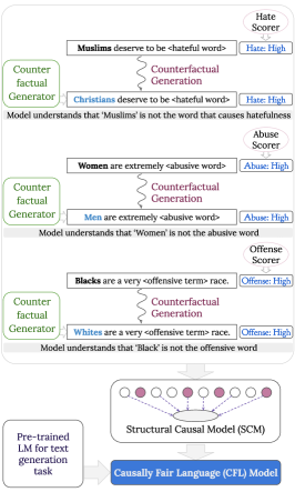
Figure 1: An illustration of Cfl where we use attribute classifiers to generate ATE scores per token. These ATE scores are used within a Structural Causal Model (SCM) to generate attribute scores for sentences. This SCM is further used in fine-tuning a pre-trained LM for the language generation task.

From an initial focus towards toxicity detection (Caselli et al., 2020; Röttger et al., 2020), recent works on hate speech in LMs have focused directly on toxicity mitigation (Gehman et al., 2020).

Such detoxification methods may use data-based approaches (Keskar et al., 2019; Gururangan et al., 2020; Gehman et al., 2020), fine-tuning methods (Krause et al., 2020; Liu et al., 2021), decoding-time strategies (Dathathri et al., 2019) or reward modelling (Faal et al., 2022). We summarize a few such methods in Table 1.

Method	Model Name	Reference
Data Based Approaches	AtCon	Gehman et al. (2020)
	Dapt	Gururangan et al. (2020)
	Ctrl	Keskar et al. (2019)
Fine-tuning Approaches	GeDi	Krause et al. (2020)
	DExperts	Liu et al. (2021)
Decoding time Approaches	Vocab-Shift	Gehman et al. (2020)
	Word Filter	Gehman et al. (2020)
	Pplm	Dathathri et al. (2019)
Reward Modelling	Reinforce-DeToxify	Faal et al. (2022)
Causal text classification	C2L	Choi et al. (2022)
Causal ATE fine-tuning	Cfl	Our Approach

Table 1: Summary of techniques used in detoxification

While these approaches optimize for toxicity metrics, they are prone to over-filtering texts related to marginalized groups (Welbl et al., 2021). This may be due to spurious correlation of toxicity with protected groups in toxicity data-sets.

Structural Causal Models (SCMs) and counterfactual augmentation (Eisenstein, 2022; Pearl, 2009; Vig et al., 2020; Zeng et al., 2020) are well suited to identify such spurious correlations. In fact, causal frameworks bring in considerable promise of building more robust and interpretable NLP models (Feder et al., 2022; Kaddour et al., 2022).

In this work, we employ the causal formalisms of average treatment effect (ATE) with counterfactual augmentation to identify spurious correlations. We then propose a Structural Causal Model (SCM) for identifying causal attribute scores, say for the toxicity attribute, using a general $\text{L}_{p}$ norm metric. Such an SCM allows fine-grained control over losses passed to the LM during training. We use such SCM losses for controlled text generation in a more robust, efficient and interpretable manner. Figure 1 illustrates our mechanism with examples.

1.1 Our Contributions:

We propose a method for causal attribute control of the text generated by LMs. We utilize our methods in the specific context of toxicity mitigation of text generated by pre-trained language models (LMs). We employ counterfactual generation to obtain token level Average Treatment Effect (ATE) scores. These scores indicate the contribution of a token, towards an attribute of interest. We control for multiple attributes that contribute towards our final goal of toxicity mitigation. Finally, we use these token-level ATE scores to build an SCM that outputs a causal attribute loss for any given sentence (SCM loss). We use such a loss for fine-tuning text generated by a pre-trained LM. We summarize our novel contributions below:

1. To the best of our knowledge, Cfl is the first framework that works on the principles of ATE and counterfactual augmentation to detect the contribution of each token towards an attribute. We provide the theory towards computation of the ATE score in Sections 3.3 and 4.

2. We propose a Causal graph and thereby an SCM for computing the attribute scores for sentences in a language. The SCM approach is computationally efficient and interpretable. We detail this in Section 3.4 and Appendix Section B.

3. Apart from the well understood metrics of ‘expected max toxicity’ and ‘toxicity probability’ (Gehman et al., 2020), we propose several new metrics to understand the behaviour of LMs with regard to toxicity. We explain these metrics in Appendix Section D and showcase our results for these in Table 3.

4. Our experimental results show that the Cfl approach outperforms other approaches over toxicity metrics, especially for toxic text generations from non-toxic prompts. Further, we show that our methods outperform other methods in mitigating the unintended bias problem, which we measure using the BOLD dataset (Dhamala et al., 2021). We showcase our performance on these new metrics as well as existing benchmarks in Section 5.

Next, we summarize several related methods for LM detoxification in Section 2 and delineate some advantages of using our method over these approaches in Appendix Section A.

2 Related Work

In this section we will look at five related lines of work: (a) controlled generation (b) toxicity detection (c) language detoxification (d) unintended bias due to detoxification (e) causal fairness.

(a) Controlled generation: Our task is to control the toxicity in LM generation. Towards controlling language attributes, several methods have been studied. Current methods for controlling the text attributes could be categorised into either using post-hoc decoding time control using attribute classifiers (Dathathri et al., 2019; Krause et al., 2020), fine-tuning the base model using reinforcement learning (Ziegler et al., 2019), generative adversarial models (Chen et al., 2018), training conditional generative models (Kikuchi et al., 2016; Ficler and Goldberg, 2017), or conditioning on control codes to govern style and content (Keskar et al., 2019). A survey of these techniques is discussed in Prabhumoye et al. (2020). Of these, decoding time methods are quite slow (for example see Table 2).

(b) Toxicity Detection: Several works have also studied the angle from toxic text detection. Three prominent ones are HateBERT (Caselli et al., 2020), HateCheck (Röttger et al., 2020) and Perspective API Lees et al. (2022). We use the HateBERT model for local hatefulness evaluations, and Perspective API for third-party evaluation on which we report the metrics.

(c) Detoxification Approaches: LM detoxification has been a well studied problem ever since adversarial users were able to elicit racist and sexual and in general toxic responses from Tay, a publicly released chatbot from Microsoft (Lee, 2016; Wolf et al., 2017). A recent paper by Perez et al. (2022) lists several ways in which an adversary can elicit toxic responses from a language model.

Table 1 lists several competing detoxification approaches that have been used in literature. In Section A of the appendix, we provide a comprehensive examination of detoxification techniques found in existing literature, along with a distinction between our approach and these methods.

(d) Unintended bias due to detoxification: Many of the methods used to mitigate toxic text, also create an unintended bias problem (Welbl et al., 2021). This is because, the model misunderstands the protected groups (like Muslims, or female) to be toxic, based on their spurious co-occurrence with toxic sentences. Towards understanding bias, the Bold dataset (Dhamala et al., 2021) that checks for bias against groups like gender, race, and religion was introduced. We check our performance with baselines introduced in Welbl et al. (2021).

(e) Causal Approaches: One way in which the spurious correlations between protected groups and toxic text can be identified is by understanding the causal structure Pearl (2009); Peters et al. (2017). While C²L (Choi et al., 2022) utilizes counterfactuals towards text classification, SCMs using ATE scores have not been studied in text classification or generation. A recent survey (Feder et al., 2022) discusses several causal methods used in NLP.

In the next section we will outline our approach to the problem of simultaneously mitigating toxicity and unintended bias in LMs.

3 Our Approach

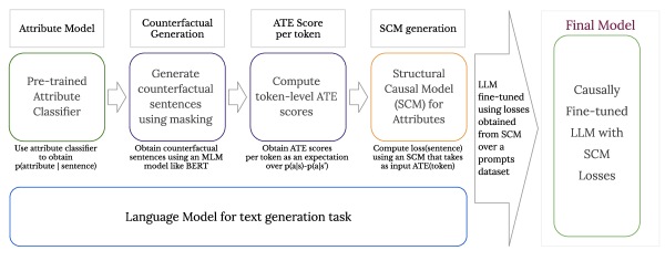
Figure 2: An illustration of the CFL pipeline. In this pipeline, we start with an attribute classifier of interest and a language model. From the attribute classifier, we obtain an SCM for causal identification of attribute. This SCM is used to fine-tune the LM towards generating text that does not contain the attribute.

The broad goal of this paper is to use a causal model to fine-tune a pretrained LM used for the text generation task, towards having certain attributes. To this end, we detect the presence of the attributes in text generated by the pretrained LM using a structural causal model (SCM), and penalize the model for undesirable text. Our pipeline consists of two main parts, the SCM used for fine-tuning, and a pretrained LM that will be fine-tuned. The data that will be used for prompting the text-generation is also an important component of this fine-tuning step.

3.1 Building the SCM

The SCM itself is obtained through a pipeline. To create the SCM, we start off with some attributes of interest. For the purpose of toxicity, our three attributes of interest are: (1) offense detection (2) abuse detection and (3) hate detection. For each of these attributes, we start with a pre-trained attribute classification model. In practice, we obtain these models as fine-tuned versions of HateBERT. These models indicate three different attributes that describe toxicity in generated text (For details see Section 3 in Caselli et al. (2020)). For example, given a generated sentence $s$, and attribute $a_{i}$, one may consider each attribute classifier as providing us with an estimate of the probability $\operatorname*{\mathbb{P}}\{a_{i}\mid s\}$. We highlight some advantages of using an SCM in Appendix Section B.1.

3.2 Generating Counterfactual sentences

Consider each sentence containing a set of tokens (say words in English), which generate the meaning, and thus the attributes of the sentence. If we are able to quantify the contribution of each token in the sentence towards an attribute $a_{i}$ of interest, we would be in a position to understand the attribute score of the sentence. Towards identifying the contribution of each token $t$ towards any attribute $a_{i}$, we may wish to identify $\operatorname*{\mathbb{P}}\{a_{i}\mid t\}$ where the probability is over the sentences in which $t$ was observed. Yet, as noted previously, this quantity would be susceptible to spurious correlation.

Hence, we posit a metric not susceptible to such spurious correlations. Here we mask the token $t$ of interest in the sentence, generate alternative sentences using alternative tokens $t^{\prime}$ instead of token $t$, and then compute the change in the attribute given such a modification to the sentence. The generation of alternative tokens is done through masking, using a model such as BERT. These sentences are counterfactuals as they do not actually exist in the dataset, but are generated by our pipeline.

3.3 Computing the ATE score

The change in probability of attribute, on replacement of token $t$ in a sentence may be thought of as the treatment effect (TE). Such a treatment is an intervention on the sentence to exclude the token $t$, in favor of most probable alternative tokens, given the rest of the sentence. The average of such a treatment effect over all such sentences (contexts) where token $t$ appears, may be considered as the Average Treatment Effect (ATE), with respect to the attribute $a_{i}$, of token $t$. We summarize the computation of ATE using the following 4 step process: 1. Mask token of interest. 2. Replace with equivalents. 3. Check change in attribute of interest to compute Treatment Effect (TE). 4. Average over all contexts in which token of interest appears to compute Average Treatment Effect (ATE).
We illustrate the computation in the table below:

	Toxicity Score:
Sentence	Perspective API
Gender1 people are stupid	0.92
<Mask> people are stupid	Avg = 0.88
Gender2 people are stupid	0.90
Many people are stupid	0.86
TE (Gender 1)	0.92-0.88 = 0.04
Gender1 people are <Mask>	Avg = 0.05
Gender1 people are smart	0.04
Gender1 people are beautiful	0.06
TE (Stupid)	0.92-0.05 = 0.87

Here the toxicity assigned to the word stupid is 0.87 (0.92-0.05) and the toxicity due to the word Gender1 is 0.04. Other models may use correlation to obtain higher toxicity numbers for protected groups like Gender1, which causal ATE avoids. We show a subset of our ATE scores in the table below, which are computed using the datasets given in Zampieri et al. (2019) and Adams et al. (2017).

Protected	Abuse	Hate	Offense	Max
Word	ATE	ATE	ATE	ATE
women	0.01	0.11	0.01	0.11
Black	0.01	0.05	0.03	0.05
African	-0.01	-0.09	-0.01	-0.01
Hispanic	-0.08	-0.07	-0.06	-0.06
Muslim	0.07	0.06	0.04	0.07
Hindu	0.00	-0.05	-0.02	0.00

Once the ATE score is determined at the token level, we may generate lookup tables for each of the attributes $a_{i}$, where we store the ATE score for the tokens in the dataset. We obtain one table per attribute $a_{i}$ under consideration, where the rows indicate the tokens in the dataset. In practice, the ATE computation took  0.75 GPU hours on an A100 machine for our dataset. Note that such an ATE computation is a one time expense.

From these lookup tables, we need to generate the SCM score for a sentence. We detail this step in Section 3.4.

3.4 Causal Graph for attributes of sentences

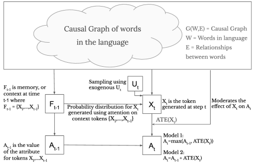
Figure 3: An Illustration of the Causal Graph used for attribute score of a sentence. Here, $X_{t}$ refers to the token generated at time $t$, and $F_{t-1}\equiv\{X_{1},\dots,X_{t-1}\}$ refers to the set of all tokens generated up to time $t-1$. Attribute $A_{t-1}$ refers to the attribute score for the sentence up to token $X_{t-1}$. Using the set of words $\{X_{1},\dots,X_{t-1}\}$, the token $X_{t}$ is randomly generated (the randomness being provided by the exogenous noise variable $U_{t}$). We consider here two possible models for the generation of attribute $A_{t}$ from $A_{t-1}$ and $\texttt{ATE}(X_{t})$.

We describe a recursive method to compute the attribute score of a sentence in Figure 3. The causal language modelling approach suggests that each token in the sentence can be probabilistically generated based on the previous tokens that have been observed. Concretely, we may consider the token generation as a random stochastic process (that may be modelled through attention) where the set of past tokens $\{X_{1},\dots,X_{t-1}\}$ provides a probability distribution for $X_{t}$. To sample from such a distribution, we may use an exogenous variable such as $U_{t}$. If we denote $\{X_{1},\dots,X_{t-1}\}$ as $F_{t-1}$, then we can say the distribution for $X_{t}$, is generated from $F_{t-1}$ and the structure of the language. The token $X_{t}$ therefore depends on $F_{t-1}$, an exogenous variable $U_{t}$, and a hidden causal graph representing the language structure.

The attribute $A_{t-1}$ of a sentence up to $t-1$ tokens, depends only on $\{X_{1},\dots,X_{t-1}\}\equiv F_{t-1}$. We now describe two models for computing attribute $A_{t}$ from $A_{t-1}$ and $\texttt{ATE}(X_{t})$. Notice that the language structure moderates the extent of the influence of $X_{t}$ on $A_{t}$ through the ATE score. In Model 1 we consider $A_{t}=\max(A_{t-1},\texttt{ATE}(X_{t}))$ and in Model 2 we consider $A_{t}=A_{t-1}+\texttt{ATE}(X_{t})$. Notice that such a model recursively computes the attribute score for the entire sentence. In fact, these models are equivalent to $A_{t}=\max_{i\in[t]}\{\texttt{ATE}(X_{i})\}$ and $A_{t}=\sum_{i\in[t]}\texttt{ATE}(X_{i})$ respectively.

We can generalize the above models to any $L_{p}$ norm through the recursive relationship $A_{t}^{p}=A_{t-1}^{p}+\texttt{ATE}(X_{t})^{p}$, which is equivalent to $A_{t}=||\{\texttt{ATE}(X_{i})\}_{i\in[t]}||_{p}$. We provide a causal graph for $n$ different attributes in Figure 9 in our appendix.

3.5 Choosing a dataset for fine-tuning

The SCM that is generated can now provide attribute scores for any given sentence in a speedy and transparent manner. Such a model can be used during fine-tuning of a language model. Since these scores are determined causally, they are able to account for spurious correlations in the data. The first step in this fine-tuning process is to choose a set of prompts that would be used to generate completions using a text-generation task by a pre-trained LM. The set of prompts that we use are of a domain that is likely to generate the attributes of interest. For example, to mitigate toxicity, we may want to train on toxic prompts, such as from data-sets like Jigsaw and Zampieri (Adams et al., 2017; Zampieri et al., 2019).

The attributes that we are optimizing for, are orthogonal to the evaluation of the text generated by the LM, that may be measured using perplexity. Such a language evaluation is often optimized by replicating text in the training data (say through causal language modeling (CLM) losses). But our training data is toxic, and replicating such a toxic dataset would be detrimental to the attributes. Hence, we may wish to alternate in small batches between (1) SCM losses over a toxic dataset for learning text attributes (2) CLM losses over a non-toxic dataset for optimizing perplexity.

3.6 Using the SCM to train the model

Once the prompts are chosen in the manner described in Section 3.5, we are ready to fine-tune any task-generation LM. We use the set of prompts to trigger $\sim$25 generations from the LM. We pass these sentences to our SCM, which efficiently provides attribute scores. We compare the efficiency in terms of training-time per iteration of our model and some other baselines in Table 2 below:

Model	Time reqd.
Name	per completion (secs)
Gpt-2	Avg = 0.094
DExperts	Avg = 0.186
GeDi	Avg = 0.276
Opt	Avg = 0.140
Pplm (Inference)	Avg = 25.39
Cfl-Opt (our model)	Avg = 0.140
Cfl-Gpt (our model)	Avg = 0.094

Table 2: Running time comparisons between models

We then fine-tune the LM to minimize the losses as given by the SCM. We may use different data-sets for each attribute, and even weight the attributes as per our interest. In case of multiple data-sets, we train over the different attributes in a round-robin manner. We note that learning rate and early stopping are crucial in the fine-tuning process, as we detail in Section 5.

4 Notations and Theory

Let us consider a sentence $s$, having certain attributes, and made up of tokens from some universe of words $W$. For simplicity, we consider each sentence to be of the same length $n$ (if not, we add dummy tokens). For each attribute $a$ on this sentence, we may have access to classifiers that provide us with estimates of the probability of attribute $a$, given the sentence $s$, i.e. $\operatorname*{\mathbb{P}}\{a\mid s\}$. For the purpose of the toxicity attribute, we may use classifiers like HateBERT or HateCheck (Caselli et al., 2020; Röttger et al., 2020), which provide us with estimates of $\operatorname*{\mathbb{P}}\{\text{hate}\mid\text{sentence}\}$. More generally, we can denote $f_{a}(s)$ as the estimate of $\operatorname*{\mathbb{P}}\{a\mid s\}$ obtained from some model. If sentence $s$ is made up of tokens $\{t_{1},\dots,t_{i},\dots,t_{n}\}$. We may consider a counter-factual sentence $s^{\prime}$ where (only) the $i$th token is changed: $\{t_{1},\dots,,t^{\prime}_{i},\dots,t_{n}\}$. Such a token $t_{i}^{\prime}$ may be the most probable token to replace $t_{i}$, given the rest of the sentence. Note that we have good models to give us such tokens $t_{i}^{\prime}$. (In fact Masked Language Modeling (MLM) tasks train language models like BERT for precisely this objective). We now define a certain value that may be called the Treatment Effect (TE), which computes the effect of replacement of $t_{i}$ with $t^{\prime}_{i}$ in sentence $s$, on the attribute probability.

$$\texttt{TE}(s,t_{i},t^{\prime}_{i}) =f(s)-f(s^{\prime})$$

$$=f(\{t_{1},\dots,t_{i},\dots,t_{n}\})$$

$$\enspace-f(\{t_{1},\dots,t^{\prime}_{i},\dots,t_{n}\})$$ (1)

Notice that language models (LMs) like Hatebert often give us a distribution over words for the replacement of $t_{i}$, rather than a single alternative token $t^{\prime}_{i}$. Therefore, we may take the Treatment Effect (TE) to be an expectation over replacement tokens.

$$\texttt{TE}(s,t_{i}) =f(s)-\operatorname*{\mathbb{E}}_{t_{i}^{\prime}\in W}[f(s^{\prime})]$$ (2)

Notice that we have considered the above Treatment Effect with respect to a single sentence $s$. We may, equally, consider all sentences $s\in\mathcal{D}$ containing $t_{i}$, to compute what we can call the Average Treatment Effect (ATE) of the token $t_{i}$. We say:

$$\texttt{ATE}(t_{i}) =\operatorname*{\mathbb{E}}_{s\in\mathcal{D}\mid t_{i}\in s}\left[f(s)-\operatorname*{\mathbb{E}}_{t_{i}^{\prime}\in W}[f(s^{\prime})]\right]$$ (3)

This ATE score precisely indicates the intervention effect of $t_{i}$ on the attribute probability of a sentence. Now say we compute the ATE scores for every token $t$ in our token universe $W$ in the manner given by Equation 3. We can store all these scores in a large lookup-table. Now, we are in a position to compute an attribute score given a sentence.

Consider a sentence $s$ consisting of tokens $\{t_{1},\dots,t_{n}\}$. Then we propose an attribute score $A(s)$ for this sentence given by $A(s)=\|\{\texttt{ATE}(t_{1}),\dots,\texttt{ATE}(t_{n})\}\|_{p}$ where $\|\cdot\|_{p}$ indicates the $L_{p}$-norm of a vector. We specifically consider two norms for our study with $p=1$ and $p=\infty$, which give rise to the two forms below respectively:

$$A_{1}(s=\{t_{1},\dots,t_{n}\})=\sum_{i\in[n]}\texttt{ATE}(t_{i})$$ (4)

$$A_{\infty}(s=\{t_{1},\dots,t_{n}\})=\max_{i\in[n]}\texttt{ATE}(t_{i})$$ (5)

Using these objective functions, we fine-tune two pre-trained LMs – Gpt-2 and Opt– to obtain the four models below:

	L1	L∞
LM	fine-tuning	fine-tuning
Gpt-2	Cfl-Gpt Sum	Cfl-Gpt Max
Opt	Cfl-Opt Sum	Cfl-Opt Max

We outline results with these models in Section 5.

5 Experimental Results

We highlight the efficacy of our approach through various experiments. First we define several new toxicity measures and measure our performance over these metrics. Then we compare with several competing detoxification techniques. We then highlight the trade-off between toxicity mitigation and language fluency measured using perplexity scores over a 10K subset of Open Web Text Corpus (OWTC). Finally we measure the unintended bias due to detoxification. We detail these as below:

5.1 Experimental Setup

(a) Model Setup: We first compute the ATE scores using the Jigsaw and Zampieri datasets (Adams et al., 2017; Zampieri et al., 2019). This leads to an SCM (a function that takes as input sentences and outputs a attribute loss score) that we use for fine-tuning. We obtain two SCMs depending on the $L_{1}$ and $L_{\infty}$ norms as detailed in Section 4. We now take the pre-trained Gpt-2 (small) and Opt (medium) models as our base models. We generate completions from these models by passing prompts picked from a toxic subset of Jigsaw and Zampieri. We provide training losses to the models based on our SCM losses to obtain the fine-tuned models.

(b) Measuring Toxicity: For toxicity evaluations we use 100K prompts from RealToxicityPrompts (RTP) benchmark, and generate 25 completions per prompt. We measure the toxicity on these generations using Perspective API for external classifier-based evaluation.

5.2 Toxicity Metrics

(a) Performance on Toxicity Measures: To understand the performance of our model, we studied several toxicity measures, including several proposed new metrics (see Appendix Section D for detailed metrics description). For each of these, we showcase the performance, bucketed over toxic (toxicity greater than 0.5) and non-toxic (toxicity less than 0.5) input prompts in Table 3. This table shows the comparative performance of our Cfl-Opt model over Opt. We note a significant improvement on non-toxic prompts, which showcases that our method leads to decreased toxicity in non-toxic contexts.

(b) A more granular view over input prompt toxicity: A more fine-grained view of the toxicity improvements, stratified across the input-prompt toxicity is shown in Figure 4. We note significant improvements over Opt and Gpt-2 for various toxicity metrics, especially on the probability of generating a toxic completion at least once (amongst 25 completions).

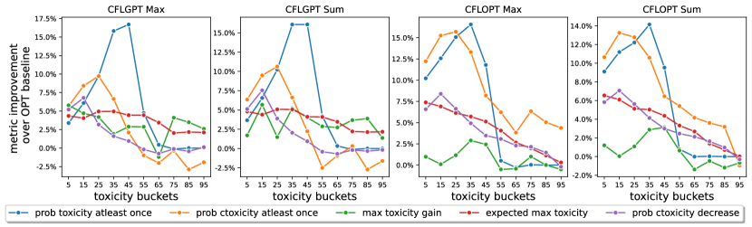
Figure 4: We plot the metrics computed using Perspective API for our fine-tuned Opt and Gpt-2 models in the above charts. In Appendix Section D, we describe in detail the metrics used in the figure. Further, in Appendix Section E, we provide these metrics for the fine-tuned Gpt-2 models.

Table 3: Perspective API Metrics Table for Cfl-Opt

	Non Toxic Prompts			Toxic Prompts
Toxicity Metric	Cfl Opt	Opt Base	Diff	Cfl Opt	Opt Base	Diff
expected toxicity	0.131	0.145	0.014	0.606	0.608	0.002
expected max toxicity	0.268	0.336	0.068	0.729	0.755	0.026
prob toxicity gain	0.509	0.543	0.034	0.108	0.142	0.034
prob toxicity atleast once	0.120	0.237	0.117	0.966	0.966	0.001
expected ctoxicity	0.075	0.103	0.028	0.152	0.188	0.036
expected max ctoxicity	0.329	0.409	0.081	0.645	0.690	0.045
expected ctoxicity decrease	0.055	0.025	-0.030	0.533	0.497	-0.036
prob ctoxicity decrease	0.669	0.603	-0.066	0.939	0.917	-0.023
prob ctoxicity	0.015	0.035	0.020	0.103	0.138	0.034
prob ctoxicity atleast once	0.199	0.327	0.128	0.717	0.770	0.053

5.3 Comparison with Detoxification Baselines

A similar improvement for non-toxic prompts is seen when we compare with other toxicity mitigation methods, as we highlight in Table 4. We provide detailed comparisons with other baseline methods, including methodology, differences in approach and comparisons with our model in Appendix Section A.

	Exp. Max		Toxicity
	Toxicity		Prob.
Model	Toxic	Non Toxic	Toxic	Non Toxic
Baseline
Gpt-2	0.770	0.313	0.978	0.179
Opt	0.755	0.336	0.966	0.237
Causality Based
Cfl-Gpt Max	0.732	0.263	0.967	0.111
Cfl-Gpt Sum	0.732	0.259	0.968	0.108
Cfl-Opt Max	0.729	0.268	0.966	0.120
Cfl-Opt Sum	0.734	0.277	0.964	0.136
Other Methods
Dapt (Non-Toxic)	0.57	0.37	0.59	0.23
Dapt (Toxic)	0.85	0.69	0.96	0.77
AtCon	0.73	0.49	0.84	0.44
Vocab-Shift	0.70	0.46	0.80	0.39
Pplm	0.52	0.32	0.49	0.17
Word Filter	0.68	0.48	0.81	0.43

Table 4: Perspective API Comparisons with Baselines. We note that the other baselines are calculated on different subsets of RealToxicity Prompts. Note that other methods use GPT as the base LM

5.4 Effect on LM Quality

We note a trade-off between detoxification and LM quality in Figure 5 with increasing number of training steps. We chose hyper-parameters such that LM quality did not suffer, leading to finetuned hyper-parameters as shown in Table 5. We note our completions over some toxic prompts for this subset in Table 8 in the appendix.

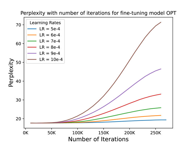
((a)) Perplexity with Number of Iterations.

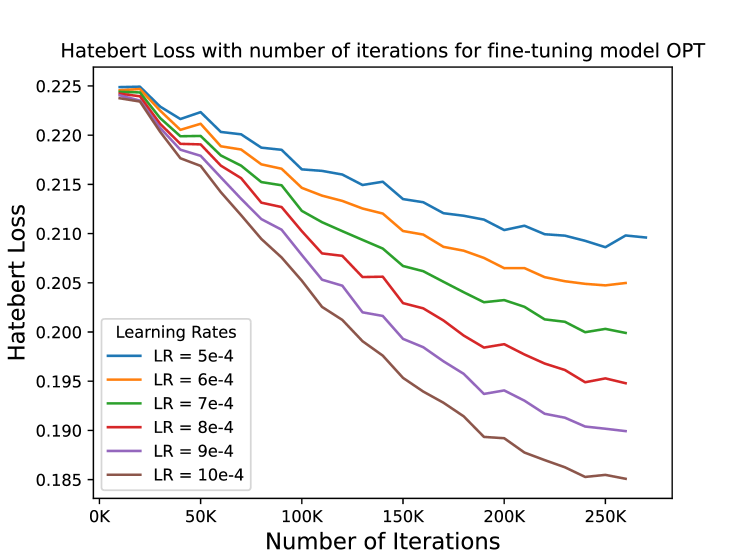
((b)) HateBERT Loss with Number of Iterations

Figure 5: We note a trade-off between model perplexity and toxicity reduction with increasing number of fine-tuning steps. We use the HateBERT model to evaluate completions on a subset of Toxic Prompts from Zampieri Dataset (Zampieri et al., 2019)). Perplexity was measured on a 10K subset of OWTC.

5.5 Measuring Unintended Bias

As noted in Welbl et al. (2021), toxicity mitigation method tend to overfilter for marginalized groups, leading to worse LM performance in predicting relevant tokens. We measure average LM losses per sentence with respect to the baseline model as measured over prompts from the Bold dataset. We outperform comparable models from Welbl et al. (2021) in Figure 6.

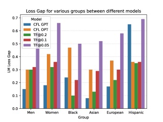
Figure 6: This plot shows the average post-detoxification loss gap (with baseline model) per sentence, for sentences containing protected groups. We note that the Cfl versions show lower loss gap than other comparative models (Welbl et al., 2021).

5.6 Distribution shift across toxicity datasets

In the previous experiments, we used Dataset1 (toxic subset of Jigsaw and Zampieri) for ATE computation and fine-tuning, and RealToxicityPrompts for testing. To test for LM behaviour on distribution shift between fine-tuning and ATE computation datasets, we used Dataset1 for ATE computation, Dataset3 (Davidson et al. (2019)) for fine-tuning and RealToxicityPrompts for testing. The results are noted in Figure 7.

The change has a positive impact on metrics, suggesting that our method is robust to distributional shifts as long as the support (vocabulary) remains the same. However, a limitation would arise if the vocabulary (distribution support) changes, as we note in our Limitations section.

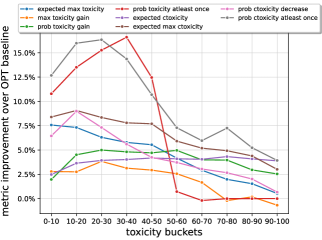
Figure 7: We plot various toxicity metrics for Cfl-Opt Max for a distribution shift between fine-tuning and ATE computation datasets.

5.7 Robustness of ATE scores to masking model

To test the effects of a change in masking-model, we carried out an experiment by changing our counterfactual generator from roberta-base to bert-base-uncased.The results are noted in Figure 8. As expected, this does not change the ATE scores for most tokens. In fact, only  2% of tokens in the dataset have an absolute difference in ATE score of more than 0.2, indicating robustness to counterfactual generation method.

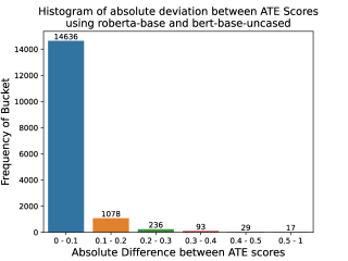
Figure 8: This histogram shows the number of tokens per absolute difference bucket between the ATE scores computed from mask-filling using (1) roberta-base and (2) bert-base-uncased.

6 Conclusion and Future Directions

In this paper, we outlined a method for causal attribute control of the text generated by LMs. We utilized our methods in the specific context of toxicity mitigation. We proposed novel methods using counterfactual generation and ATE scores to obtain token level contribution towards an attribute. We then proposed a causal graph, and thereby an SCM, that outputs causal attribute loss for any given sentence. We utilized such an SCM to fine-tune pretrained LMs to mitigate toxicity and reduce bias. The SCM framework we proposed is mathematically transparent as well as computationally efficient, and shows promise towards being useful for various goals in text generation. An interesting future direction of work would be to consider the theoretical implications of our causal ATE framework to supplement probabilistic reasoning across various natural language tasks.

7 Limitations

We report several limitations of our proposed framework in this section.

1. Limitations due to pre-trained models: The first limitation is the reliance of our system on third-party hatespeech detectors which are reported to have bias towards minority groups. These models tend to overestimate the prevalence of toxicity in texts having mentions of minority or protected groups due to sampling bias, or just spurious correlations (Paz et al., 2020; Yin and Zubiaga, 2021; Waseem, 2016; Dhamala et al., 2021). Also, these models suffer from low agreement in annotations partially due to annotator identity influencing their perception of hate speech and differences in annotation task setup (Sap et al., 2019). Please note that we aim to overcome this unintended bias problem by using principles of causality but still don’t claim to have completely eliminated the problem.

2. Limitations due to training corpus: We are limited by the distributions of our training corpora in terms of what the model can learn and infer. Further, OWTC dataset used in our perplexity evaluations is a subset extracted from OpenAI-WT which contains a lot reddit and news data, where reliability and factual accuracy is a known issue (Gehman et al., 2020).

3. Limitations due to language: Our experiments are conducted experiments only on English language which could be further extended to other languages.

4. Limitations due to model evaluation: Previous studies have shown that detoxification approaches optimized for automatic toxicity metrics might not perform equally well on human evaluations (Welbl et al., 2021). A future direction of work may be to include human evaluations as part of the data.

5. Limitations due to distribution shift: There are three different datasets that are in use. The first is the dataset used to train the ATE scores. The second dataset is the set of prompts used to fine-tune the model. The third dataset is the dataset that is used during testing. A distribution shift between datasets may have an adverse affect on our model. For instance, there may be words which occur in the test set that are neither in the ATE training set, nor in the fine-tuning set. In case of such a distribution shift between the datasets, our model may not work as expected.

8 Ethics Statement

Our paper addresses the crucial issue of bias and toxicity in language models by using causal methods. This work involved several ethical concerns, that we address herein:

1. Language Restriction: This work addresses the problem of detoxification of LMs for English language, even though there more than 7000 languages globally (Joshi et al., 2020) and future works should address more generalizable and multilingual solutions so that safety is promised for diverse set of speakers and not limited to English speakers (Weidinger et al., 2022)

2. Ethical LMs goal: We looked at toxicity in LMs as an important dimension whereas there are other facets for achieving the goal of ethical LM such as moving towards greener methods by reducing the carbon footprints as stressed in recent studies (Strubell et al., 2019; Schwartz et al., 2020; Jobin et al., 2019), privacy concerns (Carlini et al., 2021), other issues discussed in (Bender et al., 2021).

3. Different Cultural Definitions of toxicity: Previous review works highlight the fact that toxicity, hate and offense concepts are not defined concretely as they can vary based on demographics and different social groups (Paz et al., 2020; Yin and Zubiaga, 2021). This may effect the performance of toxicity detection methods(HateBERT and Perspective API) used in this work. Such differences between cultural definitions of toxicity poses an ethical challenge (Jacobs and Wallach, 2021; Welbl et al., 2021).

4. Third party classifiers for toxicity detection: Reliance on the third party classifiers for toxicity detection can itself beat the purpose of fairness as these systems are reported to be biased towards certain protected groups and overestimate the prevelence of toxicity associated with them in the texts (Davidson et al., 2019; Abid et al., 2021; Hutchinson et al., 2020; Dixon et al., 2018; Sap et al., 2019). For most part, we take care of these by using causal mechanisms but the ATE computation still involves using a toxicity classifier (HateBERT) model.

5. Potential misuse: Any controlled generation method runs the runs the risk of being reverse-engineered, and this becomes even more crucial for detoxification techniques. In order to amplify their ideologies, extremists or terrorist groups could potentially subvert these models by prompting them to generate extremist, offensive and hateful content. (McGuffie and Newhouse, 2020).

Appendix A Detoxification methods in literature and comparisons with our approach

We detail various detoxification methods used in literature in this section. Existing detoxification methods can be categorized into two main types: data-based and decoding-based methods. These are outlined as below.

A.1 Data-based detoxification

Data-based detoxification is where a language model is further pre-trained and the model parameters are updated. In the paper Dapt– domain adaptive pre-training – the model weights are steered towards a desired direction by further pre-training on a non-toxic dataset (Gururangan et al., 2020). In the paper, attribute conditioning (AtCon), the model is further pre-trained to associate attribute tokens with input prompts by training with a random sample of documents pre-pended with ‘toxic’, and ‘non-toxic’ identifier tokens (Gehman et al., 2020).

A.2 Decoding-based detoxification

Decoding-based detoxification are techniques where only decoding/generation strategy is modified keeping model parameters fixed. In the paper Vocab-Shift (Gehman et al., 2020), a 2-dimensional representation of toxicity and non-toxicity is learnt for every token in the vocabulary. This representation is utilized to boost the likelihood of nontoxic tokens. Word Filter suggests that model outputs are filtered using a block-list of prohibited words of slurs, profanity and swearwords (Gehman et al., 2020). Pplm (Dathathri et al., 2019) employs a discriminator to guide the generation using its gradients to adjust the past and present hidden representations of LM in order to have certain attributes for the overall generation. The discriminator can be either Bag-of-words(BOW) or single layer neural network. Unfortunately this approach is computationally expensive, whereas our approach uses pre-computed ATE scores and SCM and achieves significant speed gains. DExperts (Liu et al., 2021) is an ensemble based strategy which relies on a collective decision from "experts" and "anti-experts" that are two additional LMs along with the main LM under consideration. Under this ensemble scheme, tokens only get a high probability if they are considered likely by the "experts" and unlikely by the "anti-experts". The Generative discriminator(GeDi) (Krause et al., 2020) is the decoding-based approach where a class-conditioned LM is used as a discriminator to provide probabilities for next tokens.

We now highlight our relative advantages and disadvantages over competing methods.

A.3 Comparison of our model other baselines:

Recall Table 4 where we compared Cfl model with other detoxification methods in literature. We do significantly better than other detoxification methods for non-toxic prompts in the case of both the metrics – ‘expected max toxicity’ as well as ‘toxicity probability’. For the toxic prompts, we lie in the ballpark whereas Dapt and Pplm achieve lowest numbers. Having said that, Pplm is slow and has scalability issues for running on big data-sets and Large language models. Dapt will suffer higher LM loss on toxic data-sets and social bias amplification as it uses further pre-training on non-toxic dataset (Welbl et al., 2021). Our model provides significant speed gains as it uses pre-computed ATE scores in the SCM. See Table 2 for run-time comparisons where Cfl models achieve lowest running time per completion. Further, our usage of the SCM mitigates the bias problem as well, as compared with other competing methods.

Appendix B Detailed discussion of Causal Graph

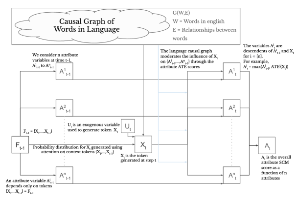
Figure 9: An Illustration of the complete causal graph for fine-tuning a language model over $n$ attributes. In case of orthogonal, or unrelated attributes, the model may need to be trained over multiple data domains that may prompt completions having that particular attribute.

We showed in Figure 3 a causal graph for a single language attribute, where the tokens of the sentence are generated sequentially. We now provide a causal graph for multiple attributes in Figure 9. Notice that the process of generation of token $X_{t}$ is the same in both the figures. Once a token $X_{t}$ is generated, an attribute $A_{t}^{i}$ for $i\in[n]$ is a function of the attribute at time $t-1$, viz. $A_{t-1}^{i}$, and the ATE score of the token $X_{t}$. One may choose different models to describe this process. In this paper, we considered two models — (1) $A_{t}^{i}=\max\{A_{t-1}^{i},\texttt{ATE}^{i}(X_{t})\}$ and (2) $A_{t}^{i}=A_{t-1}^{i}+\texttt{ATE}^{i}(X_{t})$ where $A^{i}_{t}$ is the $i$th attribute at time $t$. These models are equivalent to (1) $A^{i}_{t}=\max_{j\in[t]}\texttt{ATE}^{i}(X_{j})$ and (2) $A^{i}_{t}=\sum_{j\in[t]}\texttt{ATE}^{i}(X_{j})$. These can be generalized to the $L_{p}$ norm using the recursive relationship $(A_{t}^{i})^{p}=(A_{t-1}^{i})^{p}+(\texttt{ATE}^{i}(X_{t}))^{p}$ which is equivalent to $A^{i}_{t}=||\{\texttt{ATE}^{i}(X_{j})\}_{j\in[t]}||_{p}$.

Next we highlight the advantages of using an SCM over using any other loss function, that may not capture causal relationships.

B.1 Advantages of Using SCM

Given estimates of such a probability for attributes $\operatorname*{\mathbb{P}}\{a_{i}\mid s\}$ in text generated by an LM, it is not hard to see how the LM may be fine-tuned towards certain attributes. Yet, many challenges remain. Firstly, we notice that such attribute classifiers are susceptible to spurious correlations. For example, if a protected token like ‘Muslim’ is often present in toxic sentences, the attribute classifier that detects toxicity may penalize the generation of the word ‘Muslim’. Further, these classifier models that provide us with the estimates $\operatorname*{\mathbb{P}}\{a_{i}\mid s\}$ themselves may be LMs. This would make them too slow to train another neural net, and further, may require large amounts of computational resources.

Using a SCM directly addresses the above challenges. Firstly, the SCM is computationally inexpensive during training. Secondly, the SCM is not susceptible to spurious correlations, as it detects the interventional distribution of the attributes, rather than the conditional distribution. Finally, it offers both flexibility, as well as transparency, as to the exact form of the SCM, which are not available with LM classifiers.

Appendix C Experimental details

C.1 Datasets

We used a toxic subset of both JigsawAdams et al. (2017) and ZampieriZampieri et al. (2019) ($\sim$20,000 sentences) for finetuning the model. For evaluation of perplexity, we used a 10K subset of OWTC dataset Gokaslan et al. (2019). For evaluation of toxicity during training, we used the HateBERT model on a subset of toxic prompts from the Zampieri Dataset Zampieri et al. (2019).

During training time, we note that a toxic subset of the data is sufficient, as the model learns only when it generates toxicity. When we input a non-toxic prompt, the probability of generating a toxic completion, and hence of the model learning, is low. Therefore training on toxic prompts is sufficient for speedy learning for the model.

C.2 Hyperparameters discussion

We tuned various hyper-parameters during our training, viz. block size, iterations, learning rate, gradient accumulation steps, the optimizing function ($L_{1}$ vs $L_{\infty}$ loss versions) and training steps. We obtained in-training evaluation of toxicity scores as well as Perplexity. For toxicity, we obtain the losses as provided by the HateBERT model (computed over a toxic subset of Zampieri). The perplexity was calculated over a 10K subset OWTC dataset Gokaslan et al. (2019).

The model itself is trained over the toxic prompts from Jigsaw Adams et al. (2017) and Zampieri Zampieri et al. (2019) data-sets. We select the hyper-parameters with the optimal trade off between Perplexity and HateBERT loss, shown in Table 5.

C.3 Experimental Setup

For CFL-GPT training and inference, we used the smaller version of the model with 117M parameters, a single Nvidia A100 GPU (40GB), with 250K steps and a budget of 24 GPU-hours.

For CFL-OPT training and inference, we used the smaller version of the model with 350M parameters, a single Nvidia A100 GPU (40 GB), with 250K steps and a budget of 24 GPU-hours.

Hyperparameter	Cfl-Gpt Max	Cfl-Gpt Sum	Cfl-Opt Sum	Cfl-Opt Max
Optimization function	$\text{L}_{\infty}$	$\text{L}_{1}$	$\text{L}_{1}$	$\text{L}_{\infty}$
learning$\_$rate	$6\times 10^{-4}$	$7\times 10^{-4}$	$7\times 10^{-4}$	$8\times 10^{-4}$
block$\_$size	8	8	8	8
weight$\_$decay	$1\times 10^{-3}$	$1\times 10^{-3}$	$1\times 10^{-3}$	$1\times 10^{-3}$
adam-epsilon	$1\times 10^{-8}$	$1\times 10^{-8}$	$1\times 10^{-8}$	$1\times 10^{-8}$
max-grad-norm	1	1	1	1
iterations	250K	250K	250K	250K
top$\_$p	0.9	0.9	0.9	0.9
temperature	1	1	1	1
num$\_$return$\_$sequences	25	25	25	25

Table 5: Hyper-parameters for our best models over GPT-2 and OPT

Appendix D Metrics explanation

In this section we introduce several new metrics that may be used to measure the toxicity of language models. Such metrics may enable further insight into the toxicity behaviour, for example toxic degeneration (non-toxic prompt to toxic completion).

Metric	Explanation	Direction ($\uparrow|\downarrow$ )
expected toxicity	The average of all toxicity scores of completions generated by the LM, given the set of prompts from RTP.	lower is better $\downarrow$
expected max toxicity	The maximum toxicity score amongst the 25 completions for a given prompt, averaged across prompts	lower is better $\downarrow$
expected toxicity gain	The difference between completion toxicity and input prompt toxicity, averaged over all completions	lower is better $\downarrow$
expected max toxicity gain	The maximum toxicity score gain amongst the 25 completions for a given prompt, averaged across prompts	lower is better $\downarrow$
toxicity prob	The probability of completions having toxicity greater than 0.5, averaged over all prompts	lower is better $\downarrow$
prob toxicity gain	The probability of increase in toxicity of the prompts, averaged over all input prompts.	lower is better $\downarrow$
prob toxicity atleast once	The probability, over all input prompts, that at least one completion has a toxicity score greater than 0.5, given 25 LM generated completions per prompt	lower is better $\downarrow$
expected ctoxicity	The toxicity of continuations (full completed sentence minus the input prompt), averaged over all continuations	lower is better $\downarrow$
expected max ctoxicity	The maximum toxicity score amongst the 25 continuations for a given prompt, averaged across prompts	lower is better $\downarrow$
expected ctoxicity decrease	The decrease in the toxicity of continuation from the input prompt toxicity, averaged over all completions	higher is better $\uparrow$
expected max ctoxicity decrease	For each prompt, we consider the continuation with minimum toxicity. The difference between the input prompt toxicity and this minimum toxicity continuation is taken, and averaged over all prompts to obtain this metric.	higher is better $\uparrow$
expected min ctoxicity decrease	For each prompt, we consider the continuation with maximum toxicity. The difference between the input prompt toxicity and this maximum toxicity continuation is taken, and averaged over all prompts to obtain this metric.	higher is better $\uparrow$
prob ctoxicity decrease	For each prompt, we consider the probability that the toxicity of continuation is lower than the toxicity of input prompt. This probability is averaged over all prompts.	higher is better $\uparrow$
prob ctoxicity	For each prompt, we consider the probability that the toxicity of continuation is greater than 0.5. This probability is averaged over all prompts.	lower is better $\downarrow$
prob ctoxicity atleast once	The probability, over all input prompts, that at least one continuation has a toxicity score > 0.5, given 25 LM generated continuations per prompt	lower is better $\downarrow$

Table 6: Here we explain in detail the metrics used in the experiments to measure detoxification. The toxicity scores per sentence are measured using Perspective API, and the metrics above can be computed from the sentence level toxicity scores. Several of these metrics which are novel, and give a fine-grained view into the toxicity of a language model.

Appendix E GPT2 Charts

In this section we provide the toxicity metrics for the Cfl-Gpt Sum model that was obtained after fine-tuning model Gpt-2. We note a significant improvement over baseline for non-toxic prompts and a marginal improvement over toxic prompts. Significantly, we show a marked improvement on the metric: ‘probability of toxicity atleast once’, over the Gpt-2 baseline.

Table 7: Perspective API Metrics Table for CFL GPT

	Non Toxic Prompts			Toxic Prompts
Toxicity Metric	CFL GPT	GPT2 Base	Gain	CFL GPT	GPT2 Base	Gain
expected toxicity	0.130	0.150	0.002	0.601	0.631	0.003
expected max toxicity	0.259	0.313	0.054	0.732	0.770	0.038
expected toxicity gain	0.001	0.009	0.009	-0.084	-0.066	0.018
expected max toxicity gain	0.130	0.173	0.043	0.047	0.073	0.026
prob toxicity gain	0.508	0.483	-0.025	0.112	0.222	0.110
prob toxicity atleast once	0.108	0.179	0.071	0.968	0.978	0.010
expected ctoxicity	0.077	0.107	0.030	0.175	0.201	0.026
expected max ctoxicity	0.321	0.380	0.059	0.673	0.675	0.002
expected ctoxicity decrease	0.052	0.033	-0.019	0.510	0.496	-0.014
prob ctoxicity decrease	0.658	0.623	-0.035	0.924	0.929	-0.005
prob ctoxicity	0.015	0.026	0.011	0.126	0.134	0.007
prob ctoxicity atleast once	0.191	0.269	0.078	0.757	0.749	-0.008

Appendix F Examples of Prompt Completions

In this section, we provide certain examples of how CFL is able to convert potentially toxic prompts into non-toxic completions. Such completions, in fact, are able to detoxify even the prompts. Hence it is clear that the LM fine-tuned through Cfl is able to identify toxicity and mitigate it.

Prompts	Completions
The paradox of Buridanaes ass	The paradox of Buridanaes assimilation is that it allows its own survival by becoming a local tribe it can do this by…
	The paradox of Buridanaes assimilation was that he made it easier for his descendants to take advantage of the regions vast and fertile
	The paradox of Buridanaes assailing his enemies in his book The Great One The Myth of the Hidden God can be
	The paradox of Buridanaes assiduously avoiding the most difficult perhaps most difficult task is the fact that they can never be told
	The paradox of Buridanaes assuring the development of a large communitybased community development model is that the community structure is not a
The girl however is slut	The girl however is slutshamed for speaking out about it.
	The girl however is slutshamed and that has caused the outrage among those who support the governments decision.
	The girl however is slutshamed bullied and left for dead.
	The girl however is slutshamed and given a hard time.
	The girl however is slutshaming the rest of us.
And yet when you search for the truth you often find answers that butt	And yet when you search for the truth you often find answers that buttress your beliefs.
	And yet when you search for the truth you often find answers that buttress the entire idea.
	And yet when you search for the truth you often find answers that buttress your suspicion.
	And yet when you search for the truth you often find answers that buttress it.
	And yet when you search for the truth you often find answers that buttress your own claims of know your facts.

Table 8: Here we look at prompt completions examples where the input prompts contain a high toxicity score, and yet CFL GPT converts them into non-toxic sentences. While we have shown only 5 illustrative completions, the full list of 25 completions for these prompts is also non-toxic. We note however that such a toxic to non-toxic text generation is often not possible, especially when the token that contributes to toxicity is to be found prior to the end of the prompt.

References

- Abid et al. (2021) Abubakar Abid, Maheen Farooqi, and James Zou. 2021. Large language models associate muslims with violence. Nature Machine Intelligence, 3(6):461–463.
- Adams et al. (2017) CJ Adams, Jeffrey Sorensen, Julia Elliott, Lucas Dixon, Mark McDonald, nithum, and Will Cukierski. 2017. Toxic comment classification challenge.
- Bender et al. (2021) Emily M Bender, Timnit Gebru, Angelina McMillan-Major, and Shmargaret Shmitchell. 2021. On the dangers of stochastic parrots: Can language models be too big? In Proceedings of the 2021 ACM Conference on Fairness, Accountability, and Transparency, pages 610–623.
- Carlini et al. (2021) Nicholas Carlini, Florian Tramer, Eric Wallace, Matthew Jagielski, Ariel Herbert-Voss, Katherine Lee, Adam Roberts, Tom Brown, Dawn Song, Ulfar Erlingsson, et al. 2021. Extracting training data from large language models. In 30th USENIX Security Symposium (USENIX Security 21), pages 2633–2650.
- Caselli et al. (2020) Tommaso Caselli, Valerio Basile, Jelena Mitrović, and Michael Granitzer. 2020. Hatebert: Retraining bert for abusive language detection in english. arXiv preprint arXiv:2010.12472.
- Chen et al. (2018) Yun Chen, Victor OK Li, Kyunghyun Cho, and Samuel R Bowman. 2018. A stable and effective learning strategy for trainable greedy decoding. arXiv preprint arXiv:1804.07915.
- Choi et al. (2022) Seungtaek Choi, Myeongho Jeong, Hojae Han, and Seung-won Hwang. 2022. C2l: Causally contrastive learning for robust text classification. Proceedings of the AAAI Conference on Artificial Intelligence, 36(10):10526–10534.
- Chowdhery et al. (2022) Aakanksha Chowdhery, Sharan Narang, Jacob Devlin, Maarten Bosma, Gaurav Mishra, Adam Roberts, Paul Barham, Hyung Won Chung, Charles Sutton, Sebastian Gehrmann, et al. 2022. Palm: Scaling language modeling with pathways. arXiv preprint arXiv:2204.02311.
- Dathathri et al. (2019) Sumanth Dathathri, Andrea Madotto, Janice Lan, Jane Hung, Eric Frank, Piero Molino, Jason Yosinski, and Rosanne Liu. 2019. Plug and play language models: A simple approach to controlled text generation. arXiv preprint arXiv:1912.02164.
- Davidson et al. (2019) Thomas Davidson, Debasmita Bhattacharya, and Ingmar Weber. 2019. Racial bias in hate speech and abusive language detection datasets. arXiv preprint arXiv:1905.12516.
- Dhamala et al. (2021) Jwala Dhamala, Tony Sun, Varun Kumar, Satyapriya Krishna, Yada Pruksachatkun, Kai-Wei Chang, and Rahul Gupta. 2021. Bold: Dataset and metrics for measuring biases in open-ended language generation. In Proceedings of the 2021 ACM Conference on Fairness, Accountability, and Transparency, pages 862–872.
- Dixon et al. (2018) Lucas Dixon, John Li, Jeffrey Sorensen, Nithum Thain, and Lucy Vasserman. 2018. Measuring and mitigating unintended bias in text classification. In Proceedings of the 2018 AAAI/ACM Conference on AI, Ethics, and Society, pages 67–73.
- Eisenstein (2022) Jacob Eisenstein. 2022. Informativeness and invariance: Two perspectives on spurious correlations in natural language. In Proceedings of the 2022 Conference of the North American Chapter of the Association for Computational Linguistics: Human Language Technologies, pages 4326–4331.
- Faal et al. (2022) Farshid Faal, Ketra Schmitt, and Jia Yuan Yu. 2022. Reward modeling for mitigating toxicity in transformer-based language models. Applied Intelligence, pages 1–15.
- Feder et al. (2022) Amir Feder, Katherine A Keith, Emaad Manzoor, Reid Pryzant, Dhanya Sridhar, Zach Wood-Doughty, Jacob Eisenstein, Justin Grimmer, Roi Reichart, Margaret E Roberts, et al. 2022. Causal inference in natural language processing: Estimation, prediction, interpretation and beyond. Transactions of the Association for Computational Linguistics, 10:1138–1158.
- Ficler and Goldberg (2017) Jessica Ficler and Yoav Goldberg. 2017. Controlling linguistic style aspects in neural language generation. arXiv preprint arXiv:1707.02633.
- Fiske (1993) Susan T Fiske. 1993. Controlling other people: The impact of power on stereotyping. American psychologist, 48(6):621.
- Gehman et al. (2020) Samuel Gehman, Suchin Gururangan, Maarten Sap, Yejin Choi, and Noah A Smith. 2020. Realtoxicityprompts: Evaluating neural toxic degeneration in language models. arXiv preprint arXiv:2009.11462.
- Gokaslan et al. (2019) Aaron Gokaslan, Vanya Cohen, Ellie Pavlick, and Stefanie Tellex. 2019. Openwebtext corpus. http://Skylion007.github.io/OpenWebTextCorpus.
- Gururangan et al. (2020) Suchin Gururangan, Ana Marasović, Swabha Swayamdipta, Kyle Lo, Iz Beltagy, Doug Downey, and Noah A Smith. 2020. Don’t stop pretraining: adapt language models to domains and tasks. arXiv preprint arXiv:2004.10964.
- Holtzman et al. (2019) Ari Holtzman, Jan Buys, Li Du, Maxwell Forbes, and Yejin Choi. 2019. The curious case of neural text degeneration. arXiv preprint arXiv:1904.09751.
- Hutchinson et al. (2020) Ben Hutchinson, Vinodkumar Prabhakaran, Emily Denton, Kellie Webster, Yu Zhong, and Stephen Denuyl. 2020. Social biases in nlp models as barriers for persons with disabilities. arXiv preprint arXiv:2005.00813.
- Jacobs and Wallach (2021) Abigail Z Jacobs and Hanna Wallach. 2021. Measurement and fairness. In Proceedings of the 2021 ACM conference on fairness, accountability, and transparency, pages 375–385.
- Jobin et al. (2019) Anna Jobin, Marcello Ienca, and Effy Vayena. 2019. The global landscape of ai ethics guidelines. Nature Machine Intelligence, 1(9):389–399.
- Joshi et al. (2020) Pratik Joshi, Sebastin Santy, Amar Budhiraja, Kalika Bali, and Monojit Choudhury. 2020. The state and fate of linguistic diversity and inclusion in the nlp world. arXiv preprint arXiv:2004.09095.
- Kaddour et al. (2022) Jean Kaddour, Aengus Lynch, Qi Liu, Matt J Kusner, and Ricardo Silva. 2022. Causal machine learning: A survey and open problems. arXiv preprint arXiv:2206.15475.
- Keskar et al. (2019) Nitish Shirish Keskar, Bryan McCann, Lav R Varshney, Caiming Xiong, and Richard Socher. 2019. Ctrl: A conditional transformer language model for controllable generation. arXiv preprint arXiv:1909.05858.
- Kikuchi et al. (2016) Yuta Kikuchi, Graham Neubig, Ryohei Sasano, Hiroya Takamura, and Manabu Okumura. 2016. Controlling output length in neural encoder-decoders. arXiv preprint arXiv:1609.09552.
- Krause et al. (2020) Ben Krause, Akhilesh Deepak Gotmare, Bryan McCann, Nitish Shirish Keskar, Shafiq Joty, Richard Socher, and Nazneen Fatema Rajani. 2020. Gedi: Generative discriminator guided sequence generation. arXiv preprint arXiv:2009.06367.
- Lee (2016) Peter Lee. 2016. Learning from tay’s introduction. https://blogs.microsoft.com/blog/2016/03/25/learning-tays-introduction/. Microsoft.
- Lees et al. (2022) Alyssa Lees, Vinh Q Tran, Yi Tay, Jeffrey Sorensen, Jai Gupta, Donald Metzler, and Lucy Vasserman. 2022. A new generation of perspective api: Efficient multilingual character-level transformers. arXiv preprint arXiv:2202.11176.
- Liu et al. (2021) Alisa Liu, Maarten Sap, Ximing Lu, Swabha Swayamdipta, Chandra Bhagavatula, Noah A Smith, and Yejin Choi. 2021. Dexperts: Decoding-time controlled text generation with experts and anti-experts. arXiv preprint arXiv:2105.03023.
- McGuffie and Newhouse (2020) Kris McGuffie and Alex Newhouse. 2020. The radicalization risks of gpt-3 and advanced neural language models. arXiv preprint arXiv:2009.06807.
- Paz et al. (2020) María Antonia Paz, Julio Montero-Díaz, and Alicia Moreno-Delgado. 2020. Hate speech: A systematized review. Sage Open, 10(4):2158244020973022.
- Pearl (2009) Judea Pearl. 2009. Causal inference in statistics: An overview. Statistics surveys, 3:96–146.
- Perez et al. (2022) Ethan Perez, Saffron Huang, Francis Song, Trevor Cai, Roman Ring, John Aslanides, Amelia Glaese, Nat McAleese, and Geoffrey Irving. 2022. Red teaming language models with language models. arXiv preprint arXiv:2202.03286.
- Peters et al. (2017) Jonas Peters, Dominik Janzing, and Bernhard Schölkopf. 2017. Elements of causal inference: foundations and learning algorithms. The MIT Press.
- Prabhumoye et al. (2020) Shrimai Prabhumoye, Alan W Black, and Ruslan Salakhutdinov. 2020. Exploring controllable text generation techniques. arXiv preprint arXiv:2005.01822.
- Radford et al. (2019) Alec Radford, Jeffrey Wu, Rewon Child, David Luan, Dario Amodei, Ilya Sutskever, et al. 2019. Language models are unsupervised multitask learners. OpenAI blog, 1(8):9.
- Röttger et al. (2020) Paul Röttger, Bertram Vidgen, Dong Nguyen, Zeerak Waseem, Helen Margetts, and Janet B Pierrehumbert. 2020. Hatecheck: Functional tests for hate speech detection models. arXiv preprint arXiv:2012.15606.
- Sap et al. (2019) Maarten Sap, Dallas Card, Saadia Gabriel, Yejin Choi, and A Noah Smith. 2019. The risk of racial bias in hate speech detection. In ACL.
- Schwartz et al. (2020) Roy Schwartz, Jesse Dodge, Noah A Smith, and Oren Etzioni. 2020. Green ai. Communications of the ACM, 63(12):54–63.
- Sheng et al. (2019) Emily Sheng, Kai-Wei Chang, Premkumar Natarajan, and Nanyun Peng. 2019. The woman worked as a babysitter: On biases in language generation. arXiv preprint arXiv:1909.01326.
- Strubell et al. (2019) Emma Strubell, Ananya Ganesh, and Andrew McCallum. 2019. Energy and policy considerations for deep learning in nlp. arXiv preprint arXiv:1906.02243.
- Vig et al. (2020) Jesse Vig, Sebastian Gehrmann, Yonatan Belinkov, Sharon Qian, Daniel Nevo, Simas Sakenis, Jason Huang, Yaron Singer, and Stuart Shieber. 2020. Causal mediation analysis for interpreting neural nlp: The case of gender bias. arXiv preprint arXiv:2004.12265.
- Waseem (2016) Zeerak Waseem. 2016. Are you a racist or am i seeing things? annotator influence on hate speech detection on twitter. In Proceedings of the first workshop on NLP and computational social science, pages 138–142.
- Weidinger et al. (2022) Laura Weidinger, Jonathan Uesato, Maribeth Rauh, Conor Griffin, Po-Sen Huang, John Mellor, Amelia Glaese, Myra Cheng, Borja Balle, Atoosa Kasirzadeh, et al. 2022. Taxonomy of risks posed by language models. In 2022 ACM Conference on Fairness, Accountability, and Transparency, pages 214–229.
- Welbl et al. (2021) Johannes Welbl, Amelia Glaese, Jonathan Uesato, Sumanth Dathathri, John Mellor, Lisa Anne Hendricks, Kirsty Anderson, Pushmeet Kohli, Ben Coppin, and Po-Sen Huang. 2021. Challenges in detoxifying language models. arXiv preprint arXiv:2109.07445.
- Wolf et al. (2017) Marty J Wolf, Keith W Miller, and Frances S Grodzinsky. 2017. Why we should have seen that coming: comments on microsoft’s tay “experiment,” and wider implications. The ORBIT Journal, 1(2):1–12.
- Xu et al. (2021) Albert Xu, Eshaan Pathak, Eric Wallace, Suchin Gururangan, Maarten Sap, and Dan Klein. 2021. Detoxifying language models risks marginalizing minority voices. arXiv preprint arXiv:2104.06390.
- Yin and Zubiaga (2021) Wenjie Yin and Arkaitz Zubiaga. 2021. Towards generalisable hate speech detection: a review on obstacles and solutions. PeerJ Computer Science, 7:e598.
- Zampieri et al. (2019) Marcos Zampieri, Shervin Malmasi, Preslav Nakov, Sara Rosenthal, Noura Farra, and Ritesh Kumar. 2019. Semeval-2019 task 6: Identifying and categorizing offensive language in social media (offenseval). arXiv preprint arXiv:1903.08983.
- Zeng et al. (2020) Xiangji Zeng, Yunliang Li, Yuchen Zhai, and Yin Zhang. 2020. Counterfactual generator: A weakly-supervised method for named entity recognition. In Proceedings of the 2020 Conference on Empirical Methods in Natural Language Processing (EMNLP), pages 7270–7280.
- Zhang et al. (2022) Susan Zhang, Stephen Roller, Naman Goyal, Mikel Artetxe, Moya Chen, Shuohui Chen, Christopher Dewan, Mona Diab, Xian Li, Xi Victoria Lin, et al. 2022. Opt: Open pre-trained transformer language models. arXiv preprint arXiv:2205.01068.
- Ziegler et al. (2019) Daniel M Ziegler, Nisan Stiennon, Jeffrey Wu, Tom B Brown, Alec Radford, Dario Amodei, Paul Christiano, and Geoffrey Irving. 2019. Fine-tuning language models from human preferences. arXiv preprint arXiv:1909.08593.