Gauge theory for mixed $p$-spin glasses

Abstract

Physical quantities in the mixed $p$-spin glasses are evaluated with Nishimori’s gauge theory and several variance inequalities. The $\mathbb{Z}_{2}$-symmetry breaking and the replica-symmetry breaking are studied in finite and infinite dimensions. Obtained bounds on the expectation of the square of the magnetization and spontaneous magnetization enable us to clarify properties of paramagnetic and spin glass phases. It is proven that variances of ferromagnetic and spin glass order parameters vanish on the Nishimori line in the infinite volume limit. These results imply the self-averaging of these order parameters on the Nishimori line. The self-averaging of the spin glass order parameter rigorously justifies already argued absence of replica-symmetry breaking on the Nishimori line.

Keywords: Spin glass, Gauge invariance, Ferromagnetic long-range order, Spontaneous magnetization, Replica symmetry

1 Introduction

It is well-known that the Parisi formula [37, 38] indicates the replica-symmetry breaking (RSB) in the Sherrington-Kirkpatrick (SK) model [39]. Rigorous studies on the SK model Guerra started has had great influence on recent spin glass research in mathematical physics [24, 25]. Talagrand has developed Guerra’s square root interpolation method and has proven rigorously that the Parisi formula is exact [40, 41]. The square root interpolation method developed by Guerra and Talagrand is the standard tools for analyzing statistical mechanical models of spin glasses and artificial intelligence [4, 5, 6, 7, 8, 9, 10, 24, 25, 40, 41]. To understand RSB phenomenon, the self-averaging property and its violation of the spin overlap between different replicas should be studied. The Aizenman-Contucci and Ghirlanda-Guerra (ACGG) identities are useful to study RSB in classical spin systems [1, 16, 17, 18, 26, 41]. For example in mean field models, these identities clarify the essential property of spin overlap between different replicas in the Parisi formula in the SK model [37, 38, 41]. Toninelli has shown that the replica symmetric (RS) solution obtained by Sherrington and Kirkpatrick becomes unstable [42] in the region whose boundary is given by the Almeida-Thouless (AT) line [22]. Recently, Chen has proven an important conjecture that the RS solution becomes exact out of the AT line [15]. Also for short-range interacting models, Chatterjee has proven absence of RSB in the random field Ising model using the ACGG identities [13]. Nishimori’s gauge theory is quite useful to understand properties of disordered Ising spin systems on the Nishimori line which is a sub-manifold in the coupling constant space [33, 34]. The paramagnetic and ferromagnetic phases include the Nishimori line, where Nishimori’s gauge theory provides important informations for several physical quantities, such as the exact internal energy, bound on the specific heat and identities among correlation functions. On the Nishimori line, a local concavity of the free energy is obtained by Morita, Nishimori and Contucci [31]. Okuyama and Ohzeki obtained the Gibbs-Bogoliubov inequality for the free energy in the SK model using its local concavity on the Nishimori line [36]. These informations are quite helpful to clarify the phase structure of spin glasses in finite and infinite dimensions. The fluctuation due to random interactions is suppressed on the Nishimori line. The absence of RSB on the Nishimori line has been argued [35]. The Nishimori line gives an important notion in statistical inference problems and machine learning [10, 11] in addition to that in spin glasses.

In the present paper, several identities on the Nishimori line are derived in mixed $p$-spin glass models, and utilized them to study spin glasses. These identities represent correlation functions at an arbitrary temperature in terms of those at the corresponding point on the Nishimori line. These representations enable us to study properties of the spontaneous $\mathbb{Z}_{2}$-symmetry breaking. We show that the sample expectation of the square of the ferromagnetic magnetization and spontaneous magnetization vanish. These identities and several known inequalities imply that the variances of ferromagnetic and spin glass order parameters vanish on the Nishimori line in the infinite volume limit. These results confirm rigorously an already obtained statement that RSB does not occur on the Nishimori line [35].

2 Mixed $p$-spin glasses in finite dimensions

2.1 Definitions

For a positive integer $L$, let $\Lambda_{L}:=[0,L-1]^{d}\cap{\mathbb{Z}}^{d}$ be a $d$ dimensional cubic lattice whose volume is $|\Lambda_{L}|=L^{d}$. A spin configuration on this lattice is a mapping $\sigma:\Lambda_{L}\to\{1,-1\}$ defined by $i\mapsto\sigma_{i}=\pm 1$. Denote a product of spins

$$\sigma_{X}=\prod_{i\in X}\sigma_{i},$$

for a finite sub-lattice $X\subset\Lambda_{L}$. Let $p$ be a positive integer. To define a short-range $p$-spin Hamiltonian, define a collection ${\cal A}_{p}$ of interaction ranges $A_{p}\subset\Lambda_{L}$, such that $(0,\cdots,0)\in A_{p}$ and $|A_{p}|=p$. Define a collection ${\cal B}_{p}$ of interaction ranges by

$${\cal B}_{p}:=\{X\subset\Lambda_{L}|X=i+A_{p},i\in\Lambda_{L},A_{p}\in{\cal A}_{p}\}.$$ (1)

Let $Q$ be a finite set of positive integers. $Q$ defines a Hamiltonian of short-ranged mixed $p$-spin interactions by

$$H(\sigma,\bm{J}):=-\sum_{p\in Q}\sum_{X\in{\cal B}_{p}}J^{p}_{X}\sigma_{X},$$ (2)

where, a sequence $\bm{J}:=(J_{X}^{p})_{X\in{\cal B}_{p},p\in Q}$ consists of independent Gaussian random variables (r.v.s) with its expectation value $\mu_{p}>0$ and its standard deviation $\Delta_{p}>0$. The probability density function of each $J_{X}^{p}$ is given by

$$P_{p}(J_{X}^{p}):=\frac{1}{\sqrt{2\pi\Delta_{p}^{2}}}\exp\Big{[}-\frac{(J_{X}^{p}-\mu_{p})^{2}}{2\Delta_{p}^{2}}\Big{]}.$$ (3)

${\mathbb{E}}$ denotes the sample expectation over all $J_{X}^{p}$, such that

$${\mathbb{E}}J_{X}^{p}=\mu_{p},\ \ \ {\mathbb{E}}(J_{X}^{p}-\mu_{p})^{2}=\Delta_{p}^{2}.$$

Gaussian r.v.s $J_{X}^{p}$ for $X\in{\cal B}_{p},p\in Q$ are represented in terms of the independent and identically distributed (i.i.d.) standard Gaussian r.v.s $g_{X}^{p}$

$$J_{X}^{p}=\Delta_{p}g_{X}^{p}+\mu_{p}.$$ (4)

Note the $\mathbb{Z}_{2}$ symmetry

$$H(-\sigma,\bm{J})=H(\sigma,\bm{J}),$$ (5)

if all $p\in Q$ are even integers.

Examples of interaction ranges

Here, we give several examples of $p$-spin interactions for specific values $p=1,2,4.$ Define a distance $|i-j|$ between two sites $i:=(i_{1},i_{2},\cdots,i_{d}),j:=(j_{1},j_{2},\cdots,j_{d})\in\Lambda_{L}$ by

$$|i-j|:=\sum_{s=1}^{d}|i_{s}-j_{s}|.$$ (6)

$p=1$. In this case, the collection of all interaction ranges is given by

$${\cal A}_{1}=\{0\},\ \ \ {\cal B}_{1}=\Lambda_{L}.$$ (7)

This corresponds to a random field model.

$p=2$. In this case, a typical model has exchange interactions of nearest neighbor bonds defined by

$${\cal A}_{2}:=\{\{0,i_{2}\}|\ \ |i_{2}|=1,i_{2}\in\Lambda_{L}\},$$

$${\cal B}_{2}=\{\{i_{1},i_{2}\}|\ \ |i_{1}-i_{2}|=1,i_{s}\in\Lambda_{L},s=1,2\}.$$ (8)

The model with nearest neighbor random exchange interactions is the Edwards-Anderson model.

$p=4$. This case includes plaquette interactions defined by

$${\cal A}_{4}:=\{\{0,i_{2},i_{3},i_{4}\}|\ \ 1\leq|i_{s}|\leq 2,i_{s}\in\Lambda_{L},s=2,3,4\},$$

$${\cal B}_{4}:=\{\{i_{1},i_{2},i_{3},i_{4}\}|\ \ 1\leq|i_{s}-i_{t}|\leq 2,i_{s}\in\Lambda_{L},s,t=1,2,3,4\}.$$ (9)

Define Gibbs state for the Hamiltonian. For a positive $\beta$ and real numbers $J_{X}^{p}$, the partition function is defined by

$$Z_{L}(\beta,\bm{J}):={\rm Tr}e^{-\beta H(\sigma,\bm{J})},$$ (10)

where the trace is taken over all spin configurations. Let $f$ be an arbitrary function of spin configuration. The expectation of $f$ in the Gibbs state is given by

$$\langle f(\sigma)\rangle=\frac{1}{Z_{L}(\beta,\bm{J})}{\rm Tr}f(\sigma)e^{-\beta H(\sigma,\bm{J})}.$$ (11)

We define the following functions of $(\beta,\bm{\Delta},\bm{\mu})\in[0,\infty)^{1+2|Q|}$ and randomness $\bm{J}=(J_{X}^{p})_{X\in{\cal B}_{p},p\in Q}$

$$\psi_{L}(\beta,\bm{J}):=\frac{1}{|\Lambda_{L}|}\log Z_{L}(\beta,\bm{J}),\\$$ (12)

$-\frac{L^{d}}{\beta}\psi_{L}(\beta,\bm{J})$ is called free energy in statistical physics. Define a function $p_{L}:[0,\infty)^{1+2|Q|}\rightarrow{\mathbb{R}}$ by

$$p_{L}(\beta,\bm{\Delta},\bm{\mu}):={\mathbb{E}}\psi_{L}(\beta,\bm{J}).$$ (13)

Note that the function $\psi_{L}(\beta,\bm{J})$ and $p_{L}(\beta,\bm{\Delta},\bm{\mu})$ are convex functions of each variable.

To study ferromagnetic phase transition, define an extended $p$-th ferromagnetic order parameter.

$$m^{p}:=\frac{1}{|{\cal B}_{p}|}\sum_{X\in{\cal B}_{p}}\sigma_{X}$$ (14)

To study replica-symmetry and its breaking, define $n$ replicated spin configurations $(\sigma^{a})_{a=1,\cdots,n}$ and a replica symmetric Hamiltonian

$$H(\sigma^{1},\cdots,\sigma^{n},\bm{J}):=\sum_{a=1}^{n}H(\sigma^{a},\bm{J}),$$ (15)

which is invariant under an arbitrary permutation $s\in S_{n}$

$$H(\sigma^{1},\cdots,\sigma^{n},\bm{J})=H(\sigma^{s(1)},\cdots,\sigma^{s(n)},\bm{J}).$$

We assume replica symmetric boundary condition throughout the present paper. The covariance of $p$-spin interaction in two replicated Hamiltonians with indices $a,b\leq n$ is defined by the following expectation over the sequence $\bm{J}^{p}$ of Gaussian r.v.s

$$\sum_{X,Y\in{\cal B}_{p}}{\mathbb{E}}J_{X}^{p}\sigma_{X}^{a}J_{Y}^{p}\sigma_{Y}^{b}-\sum_{X,Y\in{\cal B}_{p}}{\mathbb{E}}J_{X}^{p}\sigma_{X}^{a}{\mathbb{E}}J_{Y}^{p}\sigma_{Y}^{b}=|{\cal B}_{p}|\Delta_{p}^{2}R^{p}_{a,b},$$ (16)

where the $p$-th overlap $R^{p}_{a,b}$ is defined by

$$R^{p}_{a,b}:=\frac{1}{|{\cal B}_{p}|}\sum_{X\in{\cal B}_{p}}\sigma^{a}_{X}\sigma^{b}_{X}.$$

For example, $p=1$ spin interaction with ${\cal B}_{1}=\Lambda_{L}$ is the random field Zeeman energy, and the corresponding overlap becomes the site overlap

$$R^{1}_{a,b}=\frac{1}{|\Lambda_{L}|}\sum_{i\in\Lambda_{L}}\sigma^{a}_{i}\sigma^{b}_{i}.$$

The $p=2$ spin interaction with a set ${\cal B}_{2}:=\{\{i,j\}|i,j\in\Lambda_{L},|i-j|=1\}$ of nearest neighbor bonds is the bond exchange interactions, it becomes the bond overlap

$$R^{2}_{a,b}=\frac{1}{|{\cal B}_{2}|}\sum_{X\in{\cal B}_{2}}\sigma_{X}^{a}\sigma^{b}_{X}=\frac{1}{L^{d}d}\sum_{|i-j|=1}\sigma_{i}^{a}\sigma^{a}_{j}\sigma^{b}_{i}\sigma^{b}_{j}.$$

In short-range spin glass models, for example the Edwards-Anderson model [23] the bond overlap is independent of the site overlap unlike the SK model [39], where the bond overlap is identical to the square of the site overlap.

Define the Nishimori manifold (NM) by

$$\beta\Delta_{p}^{2}=\mu_{p},$$ (17)

for all $p\in Q$ in the coupling constant space of $(\beta,\bm{\Delta},\bm{\mu})\in[0,\infty)^{1+2|Q|}$.

2.2 $\mathbb{Z}_{2}$-symmetry breaking

Let us define a gauge transformation in Nishimori’s gauge theory for spin glass [19, 31, 34]. For a spin configuration $\tau\in\{1,-1\}^{\Lambda_{L}}$, define a gauge transformation by

$$J_{X}^{p}\to J_{X}^{p}\tau_{X},\ \ \ \sigma_{X}\to\sigma_{X}\tau_{X}.$$ (18)

The Hamiltonian is invariant under the gauge transformation.

$$H(\sigma\tau,\bm{J}\tau)=H(\sigma,\bm{J}).$$ (19)

The distribution function is transformed into

$$P_{p}(J_{X}^{p}\tau_{X})=\tilde{P}_{p}(J_{X}^{p})e^{\frac{\mu_{p}}{\Delta_{p}^{2}}J_{X}^{p}\tau_{X}},$$ (20)

where

$$\tilde{P}_{p}(J_{X}^{p}):=\frac{1}{\sqrt{2\pi\Delta_{p}^{2}}}\exp\Big{[}-\frac{(J_{X}^{p})^{2}+(\mu_{p})^{2}}{2\Delta_{p}^{2}}\Big{]}.$$

It is well-known that the expectation of the Hamiltonian on NM is given by

$$\mathbb{E}\langle H\rangle=-\sum_{p\in Q}|{\cal B}_{p}|\mu_{p}.$$ (21)

The following properties of correlation functions on NM are shown in Ref.[7, 31, 34].

Lemma 2.1

Denote $\beta_{\rm N}:=\mu_{p}/\Delta_{p}^{2}$ for all $p\in Q$, then $\beta$ is identical to $\beta_{\rm N}$ on the NM. Denote the Gibbs expectation of an arbitrary function $f:\Sigma_{L}\to{\mathbb{R}}$ of spin configuration

$$\langle f(\sigma)\rangle_{\beta}$$

at an inverse temperature $\beta$, if it is necessary. On NM, one point function for $X\in{\cal B}_{p}$ satisfies

$$\mathbb{E}\langle\sigma_{X}\rangle_{\beta}=\mathbb{E}\langle\sigma_{X}\rangle_{\beta}\langle\sigma_{X}\rangle_{\beta_{\rm N}},$$ (22)

and two point functions for $X,Y\in{\cal B}_{p}$ satisfy

$$\mathbb{E}\langle\sigma_{X}\rangle_{\beta}\langle\sigma_{Y}\rangle_{\beta}=\mathbb{E}\langle\sigma_{X}\rangle_{\beta}\langle\sigma_{Y}\rangle_{\beta}\langle\sigma_{X}\sigma_{Y}\rangle_{\beta_{\rm N}},\ \ \ \mathbb{E}\langle\sigma_{X}\sigma_{Y}\rangle_{\beta}=\mathbb{E}\langle\sigma_{X}\sigma_{Y}\rangle_{\beta}\langle\sigma_{X}\sigma_{Y}\rangle_{\beta_{\rm N}}.$$ (23)

An arbitrary multiple point function satisfies an extended formula.

Theorem 2.2

Consider the model with $Q=\{1,2\}$ for an arbitrary $\beta>0$, and define $\beta_{\rm N}:=\frac{\mu_{2}}{\Delta_{2}^{2}}$. The sample expectation of square of the ferromagnetic magnetization vanishes for any $(\beta,0,\Delta_{2},0,\mu_{2})$,

$$\lim_{L\to\infty}\mathbb{E}\langle(m^{1})^{2}\rangle_{\beta}=0,$$ (24)

if the quenched expectation of square of magnetization vanishes $\displaystyle\lim_{L\to\infty}\mathbb{E}\langle(m^{1})^{2}\rangle_{\beta_{\rm N}}=0,$ for $(\beta_{\rm N},0,\Delta_{2},0,\mu_{2})$ on NM.
There is no spontaneous magnetization for any $(\beta,\sqrt{\frac{\mu_{1}}{\beta_{\rm N}}},\Delta_{2},\mu_{1},\mu_{2}),$

$$\lim_{\mu_{1}\searrow 0}\lim_{L\to\infty}\mathbb{E}\langle m^{1}\rangle_{\beta}=\lim_{\mu_{1}\searrow 0}\lim_{L\to\infty}\Big{[}\frac{1}{\beta}\frac{\partial}{\partial\mu_{1}}p_{L}(\beta,\Delta_{1},\Delta_{2},\mu_{1},\mu_{2})\Big{]}_{\Delta_{1}=\sqrt{\frac{\mu_{1}}{\beta_{\rm N}}}}=0,$$ (25)

if there is no spontaneous magnetization $\displaystyle\lim_{\mu_{1}\searrow 0}\lim_{L\to\infty}\mathbb{E}\langle m^{1}\rangle_{\beta_{\rm N}}=0$ for $(\beta_{\rm N},\sqrt{\frac{\mu_{1}}{\beta_{\rm N}}},\Delta_{2},\mu_{1},\mu_{2})$.

Proof.

The first claim has been indicated by Nishimori [34]. Here, we prove this claim. The identity (23) implies

$$\mathbb{E}\langle(m^{1})^{2}\rangle_{\beta} = \frac{1}{|\Lambda_{L}|^{2}}\sum_{i,j\in\Lambda_{L}}\mathbb{E}\langle\sigma_{i}\sigma_{j}\rangle_{\beta}=\frac{1}{|\Lambda_{L}|^{2}}\sum_{i,j\in\Lambda_{L}}\mathbb{E}\langle\sigma_{i}\sigma_{j}\rangle_{\beta}\langle\sigma_{i}\sigma_{j}\rangle_{\beta_{\rm N}}$$ (26)

$$\leq \frac{1}{|\Lambda_{L}|^{2}}\sum_{i,j\in\Lambda_{L}}\mathbb{E}|\langle\sigma_{i}\sigma_{j}\rangle_{\beta}||\langle\sigma_{i}\sigma_{j}\rangle_{\beta_{\rm N}}|\leq\frac{1}{|\Lambda_{L}|^{2}}\sum_{i,j\in\Lambda_{L}}\mathbb{E}|\langle\sigma_{i}\sigma_{j}\rangle_{\beta_{\rm N}}|$$

$$\leq \frac{1}{|\Lambda_{L}|^{2}}\sum_{i,j\in\Lambda_{L}}\sqrt{\mathbb{E}\langle\sigma_{i}\sigma_{j}\rangle_{\beta_{\rm N}}}\leq\sqrt{\frac{1}{|\Lambda_{L}|^{2}}\sum_{i,j\in\Lambda_{L}}\mathbb{E}\langle\sigma_{i}\sigma_{j}\rangle_{\beta_{\rm N}}}$$

$$\leq \sqrt{\mathbb{E}\langle(m^{1})^{2}\rangle_{\beta_{\rm N}}},$$

Therefore, the assumption implies

$$\lim_{L\to\infty}\mathbb{E}\langle(m^{1})^{2}\rangle_{\beta}=0,$$ (27)

also for $(\beta,0,\Delta_{2},0,\mu_{2})$. The identity (22) and the Cauchy-Schwarz inequality give a bound on the magnetization for $(\beta,\sqrt{\frac{\mu_{1}}{\beta_{\rm N}}},\Delta_{2},\mu_{1},\mu_{2})$

$$|{\mathbb{E}}\langle\sigma_{i}\rangle_{\beta}|=|{\mathbb{E}}\langle\sigma_{i}\rangle_{\beta}\langle\sigma_{i}\rangle_{\beta_{\rm N}}|\leq{\mathbb{E}}|\langle\sigma_{i}\rangle_{\beta}||\langle\sigma_{i}\rangle_{\beta_{\rm N}}|\leq{\mathbb{E}}|\langle\sigma_{i}\rangle_{\beta_{\rm N}}|\leq\sqrt{{\mathbb{E}}\langle\sigma_{i}\rangle_{\beta_{\rm N}}^{2}}=\sqrt{{\mathbb{E}}\langle\sigma_{i}\rangle_{\beta_{\rm N}}},$$ (28)

for any $i\in\Lambda_{L}$. This and Jensen’s inequality imply

$$|\mathbb{E}\langle m^{1}\rangle_{\beta}|\leq\frac{1}{|\Lambda_{L}|}\sum_{i\in\Lambda_{L}}|{\mathbb{E}}\langle\sigma_{i}\rangle_{\beta}|\leq\frac{1}{|\Lambda_{L}|}\sum_{i\in\Lambda_{L}}\sqrt{{\mathbb{E}}\langle\sigma_{i}\rangle_{\beta_{\rm N}}}\leq\sqrt{\frac{1}{|\Lambda_{L}|}\sum_{i\in\Lambda_{L}}{\mathbb{E}}\langle\sigma_{i}\rangle_{\beta_{\rm N}}}=\sqrt{{\mathbb{E}}\langle m^{1}\rangle_{\beta_{\rm N}}}.$$ (29)

Therefore, the assumption on the spontaneous magnetization on NM implies that there is no spontaneous magnetization for an arbitrary $\beta>0$

$$\lim_{\mu_{1}\searrow 0}\lim_{L\to\infty}\mathbb{E}\langle m^{1}\rangle_{\beta}\leq\lim_{\mu_{1}\searrow 0}\lim_{L\to\infty}\mathbb{E}\langle m^{1}\rangle_{\beta_{\rm N}}=0.$$ (30)

This completes the proof. $\Box$

Note 2.3

Theorem 2.2 is valid also in the model with $Q\supsetneq\{1,2\}$, if the sample expectation of the square of magnetization and spontaneous magnetization vanish on the NM in this model.
Theorem 2.2 is proven also in quantum spin glasses, for example in the Edwards-Anderson model with quantum mechanical perturbations [30]. These results are well-known general properties of spin glasses, which are consistent with rounding effects obtained in Ref. [2, 3, 27]. Nishimori’s gauge theory is useful also for disordered quantum spin systems [32].

2.3 Self-averaging of order parameters on the NM

Lemma 2.4

For any $p\in Q$ and for any $\Delta_{p}>0$, the variance of the ferromagnetic order parameter vanishes

$$\lim_{L\rightarrow\infty}{\mathbb{E}}\langle(m^{p}-\langle m^{p}\rangle)^{2}\rangle=0.$$ (31)

On the NM, the variance of the overlap vanishes

$$\lim_{L\to\infty}\mathbb{E}\langle(R_{1,2}^{p}-\langle R_{1,2}^{p}\rangle)^{2}\rangle=0.$$ (32)

in the infinite volume limit.
Proof.

For any positive integer $k$, any $p\in Q$ and any $X\in{\cal B}_{p}$, the summation over truncated correlation functions has an upper bound [12, 28]

$$\sum_{Y_{1},\cdots,Y_{k}\in{\cal B}_{p}}(\mathbb{E}\langle\sigma_{X};\sigma_{Y_{1}};\cdots;\sigma_{Y_{k}}\rangle)^{2}\leq k!(\beta\Delta_{p})^{-2k}.$$ (33)

The inequality (33) for $k=1$ implies

$$\sum_{Y\in{\cal B}_{p}}[\mathbb{E}(\langle\sigma_{X}\sigma_{Y}\rangle-\langle\sigma_{X}\rangle\langle\sigma_{Y}\rangle)]^{2}\leq(\beta\Delta_{p})^{-2}.$$ (34)

This and the Cauchy-Schwarz inequality imply

$$\sum_{Y\in{\cal B}_{p}}|\mathbb{E}(\langle\sigma_{X}\sigma_{Y}\rangle-\langle\sigma_{X}\rangle\langle\sigma_{Y}\rangle)|\leq\sqrt{\sum_{Y\in{\cal B}_{p}}[\mathbb{E}(\langle\sigma_{X}\sigma_{Y}\rangle-\langle\sigma_{X}\rangle\langle\sigma_{Y}\rangle)]^{2}\sum_{Y\in{\cal B}_{p}}1^{2}}\leq\frac{\sqrt{|{\cal B}_{p}|}}{\beta\Delta_{p}}.$$ (35)

From the above inequality, the variance of the ferromagnetic order parameter is obtained

$$\lim_{L\to\infty}{\mathbb{E}}\langle(m^{p}-\langle m^{p}\rangle)^{2}\rangle=\lim_{L\to\infty}\frac{1}{|{\cal B}_{p}|^{2}}\sum_{X,Y\in{\cal B}_{p}}\mathbb{E}(\langle\sigma_{X}\sigma_{Y}\rangle-\langle\sigma_{X}\rangle\langle\sigma_{Y}\rangle)\leq\lim_{L\to\infty}\frac{1}{\beta\Delta_{p}\sqrt{|{\cal B}_{p}|}}=0,$$ (36)

since $|{\cal B}_{p}|$ is proportional to $|\Lambda_{L}|$. This gives the first identity (31). The inequality (33) for $k=3$ for the summation over $Y_{1}=X$ and $Y_{2}=Y_{3}=Y$ implies

$$\sum_{Y\in{\cal B}_{p}}[\mathbb{E}(\langle\sigma_{X}\sigma_{Y}\rangle^{2}-4\langle\sigma_{X}\rangle\langle\sigma_{Y}\rangle\langle\sigma_{X}\sigma_{Y}\rangle+3\langle\sigma_{X}\rangle^{2}\langle\sigma_{Y}\rangle^{2})]^{2}\leq\frac{3}{2}(\beta\Delta_{p})^{-6}.$$ (37)

Therefore,

$$\sum_{Y\in{\cal B}_{p}}|\mathbb{E}(\langle\sigma_{X}\sigma_{Y}\rangle^{2}-4\langle\sigma_{X}\rangle\langle\sigma_{Y}\rangle\langle\sigma_{X}\sigma_{Y}\rangle+3\langle\sigma_{X}\rangle^{2}\langle\sigma_{Y}\rangle^{2})|\leq\frac{1}{\beta^{3}\Delta_{p}^{3}}\sqrt{\frac{3|{\cal B}_{p}|}{2}}.$$ (38)

On the NM, this inequality is represented as

$$\sum_{Y\in{\cal B}_{p}}|\mathbb{E}(\langle\sigma_{X}\sigma_{Y}\rangle-4\langle\sigma_{X}\rangle\langle\sigma_{Y}\rangle+3\langle\sigma_{X}\rangle^{2}\langle\sigma_{Y}\rangle^{2})|\leq\frac{1}{\beta_{\rm N}^{3}\Delta_{p}^{3}}\sqrt{\frac{3|{\cal B}_{p}|}{2}}.$$ (39)

This and the inequality (35) imply

$$\sum_{Y\in{\cal B}_{p}}|\mathbb{E}(\langle\sigma_{X}\rangle^{2}\langle\sigma_{Y}\rangle^{2}-\langle\sigma_{X}\rangle\langle\sigma_{Y}\rangle)|$$

$$=\frac{1}{3}\sum_{Y\in{\cal B}_{p}}|\mathbb{E}(-\langle\sigma_{X}\sigma_{Y}\rangle+\langle\sigma_{X}\rangle\langle\sigma_{Y}\rangle+\langle\sigma_{X}\sigma_{Y}\rangle-4\langle\sigma_{X}\rangle\langle\sigma_{Y}\rangle+3\langle\sigma_{X}\rangle^{2}\langle\sigma_{Y}\rangle^{2})|$$

$$\leq\frac{1}{3}\sum_{Y\in{\cal B}_{p}}|\mathbb{E}(\langle\sigma_{X}\sigma_{Y}\rangle-\langle\sigma_{X}\rangle\langle\sigma_{Y}\rangle)|+\frac{1}{3}\sum_{Y\in{\cal B}_{p}}|{\mathbb{E}}(\langle\sigma_{X}\sigma_{Y}\rangle-4\langle\sigma_{X}\rangle\langle\sigma_{Y}\rangle+3\langle\sigma_{X}\rangle^{2}\langle\sigma_{Y}\rangle^{2})|$$

$$\leq\Big{(}\frac{1}{3}+\frac{1}{\sqrt{6}\beta_{\rm N}^{2}\Delta_{p}^{2}}\Big{)}\frac{\sqrt{|{\cal B}_{p}|}}{\beta_{\rm N}\Delta_{p}},$$ (40)

and

$$\sum_{Y\in{\cal B}_{p}}\mathbb{E}(\langle\sigma_{X}\sigma_{Y}\rangle^{2}-\langle\sigma_{X}\rangle^{2}\langle\sigma_{Y}\rangle^{2})$$

$$=\sum_{Y\in{\cal B}_{p}}\mathbb{E}(\langle\sigma_{X}\sigma_{Y}\rangle-\langle\sigma_{X}\rangle\langle\sigma_{Y}\rangle+\langle\sigma_{X}\rangle\langle\sigma_{Y}\rangle-\langle\sigma_{X}\rangle^{2}\langle\sigma_{Y}\rangle^{2})$$

$$\leq\sum_{Y\in{\cal B}_{p}}|\mathbb{E}(\langle\sigma_{X}\sigma_{Y}\rangle-\langle\sigma_{X}\rangle\langle\sigma_{Y}\rangle)|+\sum_{Y\in{\cal B}_{p}}|\mathbb{E}(\langle\sigma_{X}\rangle\langle\sigma_{Y}\rangle-\langle\sigma_{X}\rangle^{2}\langle\sigma_{Y}\rangle^{2})|$$

$$\leq\Big{(}\frac{4}{3}+\frac{1}{\sqrt{6}\beta_{\rm N}^{2}\Delta_{p}^{2}}\Big{)}\frac{\sqrt{|{\cal B}_{p}|}}{\beta_{\rm N}\Delta_{p}}.$$ (41)

The following variance of overlap is bounded by

$$\mathbb{E}\langle(R_{1,2}^{p}-\langle R_{1,2}^{p}\rangle)^{2}\rangle = \frac{1}{|{\cal B}_{p}|^{2}}\sum_{X,Y\in{\cal B}_{p}}\mathbb{E}(\langle\sigma_{X}\sigma_{Y}\rangle^{2}-\langle\sigma_{X}\rangle^{2}\langle\sigma_{Y}\rangle^{2})$$ (42)

$$\leq \Big{(}\frac{4}{3}+\frac{1}{\sqrt{6}\beta_{\rm N}^{2}\Delta_{p}^{2}}\Big{)}\frac{1}{\beta_{\rm N}\Delta_{p}\sqrt{|{\cal B}_{p}|}}.$$ (43)

Since $|{\cal B}_{p}|$ is proportional to $L^{d}$ for any $p\in Q$, the variance of the overlap vanishes on the NM in the infinite-volume limit

$$\lim_{L\to\infty}\mathbb{E}\langle(R_{1,2}^{p}-\langle R_{1,2}^{p}\rangle)^{2}\rangle=0.$$ (44)

This completes the proof. $\Box$

The following lemma has been given by Aizenman-Contucci and Ghirlanda-Guerra independently [1, 26].

Lemma 2.5

(Aizenman-Contucci-Ghirlanda-Guerra identities) Let $f:\Sigma_{L}^{n}\to{\mathbb{R}}$ be a bounded function, where $\Sigma_{L}:=\{-1,1\}^{\Lambda_{L}}$ is a set of all spin configurations. The Aizenman-Contucci-Ghirlanda-Guerra (ACGG) identities give

$$\lim_{L\to\infty}(\mathbb{E}\langle fR_{1,n+1}^{p}\rangle-\frac{1}{n}\mathbb{E}\langle f\rangle\mathbb{E}\langle R_{1,2}^{p}\rangle-\frac{1}{n}\sum_{a=2}^{n}\mathbb{E}\langle fR_{1,a}^{p}\rangle)=0,$$ (45)

for any bounded $f$, for any $p\in Q$ and for almost all $\Delta_{p}>0$.
Proof.

The proof is given in several literatures [1, 12, 13, 16, 17, 18, 19, 26, 28, 29, 41]. The ACGG identities are proven on the basis of the self-averaging property of $\psi_{L}(\beta,\bm{J})$ and the convexity of

$$p(\beta,\bm{\Delta},\bm{\mu}):=\lim_{L\to\infty}p_{L}(\beta,\bm{\Delta},\bm{\mu}),$$

with respect to $\Delta_{p}$. $\Box$

Theorem 2.6

For any $p\in Q$, for almost all $\mu_{p}>0$, the variance of the ferromagnetic order parameter vanishes

$$\lim_{L\rightarrow\infty}{\mathbb{E}}\langle(m^{p}-{\mathbb{E}}\langle m^{p}\rangle)^{2}\rangle=0,$$ (46)

in the infinite volume limit. For any $p\in Q$, for almost all $\Delta_{p}>0$ on the NM, the variance of the overlap vanishes

$$\lim_{L\rightarrow\infty}{\mathbb{E}}\langle(R_{1,2}^{p}-{\mathbb{E}}\langle R_{1,2}^{p}\rangle)^{2}\rangle=0,$$ (47)

in the infinite volume limit.

Proof.

The self-averaging property of the magnetization $\langle m^{p}\rangle$ for almost all $\mu_{p}>0$ is proven as in the same method to prove the ACGG identities. The proof is given on the basis of the self-averaging property of $\psi_{L}(\beta,\bm{J})$ and convexity of $p(\beta,\bm{\Delta},\bm{\mu})$ with respect to $\mu_{p}$ [19, 28].
Here, we prove the self-averaging property of the overlap on NM.
For $n=2,f=R_{1,2}^{p}$, ACGG identities (45) give

$$\lim_{L\to\infty}[\mathbb{E}\langle R_{1,2}^{p}R_{1,3}^{p}\rangle-\frac{1}{2}(\mathbb{E}\langle R_{1,2}^{p}\rangle)^{2}-\frac{1}{2}\mathbb{E}\langle(R_{1,2}^{p})^{2}\rangle]=0.$$ (48)

For $n=3,f=R_{2,3}$,

$$\lim_{L\to\infty}[\mathbb{E}\langle R_{2,3}^{p}R_{1,4}^{p}\rangle-\frac{1}{3}\mathbb{E}\langle R_{2,3}^{p}\rangle\mathbb{E}\langle R_{1,2}^{p}\rangle-\frac{1}{3}\mathbb{E}\langle R_{2,3}^{p}R_{1,2}^{p}\rangle-\frac{1}{3}\mathbb{E}\langle R_{2,3}^{p}R_{1,3}^{p}\rangle]=0.$$ (49)

The replica symmetry implies $\langle R_{2,3}^{p}\rangle=\langle R_{1,2}^{p}\rangle$,

$$\langle R_{2,3}^{p}R_{1,2}^{p}\rangle=\langle R_{2,3}^{p}R_{1,3}^{p}\rangle=\langle R_{1,3}^{p}R_{1,2}^{p}\rangle,$$

and $\langle R_{2,3}^{p}R_{1,4}^{p}\rangle=\langle R_{1,2}^{p}\rangle^{2}$, then we have

$$\lim_{L\to\infty}[\mathbb{E}\langle R_{1,2}^{p}\rangle^{2}-\frac{1}{3}(\mathbb{E}\langle R_{1,2}^{p}\rangle)^{2}-\frac{2}{3}\mathbb{E}\langle R_{1,3}^{p}R_{1,2}^{p}\rangle]=0.$$ (50)

Substitute the identity (48) into (50), then we have

$$\lim_{L\to\infty}[\mathbb{E}\langle R_{1,2}^{p}\rangle^{2}-\frac{2}{3}(\mathbb{E}\langle R_{1,2}^{p}\rangle)^{2}-\frac{1}{3}\mathbb{E}\langle(R_{1,2}^{p})^{2}\rangle]=0.$$

For two deviations $R_{1,2}^{p}-{\mathbb{E}}\langle R_{1,2}^{p}\rangle$ and $R_{1,2}^{p}-\langle R_{1,2}^{p}\rangle$, there are relations between two variances

$$2\lim_{L\rightarrow\infty}{\mathbb{E}}\langle(R_{1,2}^{p}-{\mathbb{E}}\langle R_{1,2}^{p}\rangle)^{2}\rangle=3\lim_{L\rightarrow\infty}{\mathbb{E}}\langle(R_{1,2}^{p}-\langle R_{1,2}^{p}\rangle)^{2}\rangle,$$ (51)

This and the identity (32) imply

$$\lim_{L\rightarrow\infty}{\mathbb{E}}\langle(R_{1,2}^{p}-{\mathbb{E}}\langle R_{1,2}^{p}\rangle)^{2}\rangle=0,$$ (52)

for any $p\in Q$ and for almost all $\Delta_{p}>0$ on the NM. This has proven Theorem 2.6. $\Box$

Example:

Consider a model defined by $Q:=\{1,2\}$, ${\cal B}_{1}:=\Lambda_{L}$ and nearest neighbor bonds ${\cal B}_{2}:=\{\{i,j\}|i,j\in\Lambda_{L},|i-j|=1,\}$. This model is the random field Edwards-Anderson model. Theorem 2.6 is still valid in a $\mathbb{Z}_{2}$-symmetric limit $\Delta_{1}\to 0$ on the NM defined by $\beta_{\rm N}=\mu_{1}/\Delta_{1}^{2}=\mu_{2}/\Delta_{2}^{2}$, even though spontaneous $\mathbb{Z}_{2}$ symmetry breaking appears.

3 Mean field mixed $p$-spin glasses

3.1 Definitions

Let $L$ be a positive integer and define $\Lambda_{L}:=[1,L]\cap\mathbb{Z}$. A collection

$${\cal B}_{p}:=\{X\subset\Lambda_{L}||X|=p\},$$

consists of all subsets of $\Lambda_{L}$ with cardinality $p$. Mean field mixed $p$-spin glass model is defined by

$$H(\sigma,\bm{J}):=-\sum_{p\in Q}\sum_{X\in{\cal B}_{p}}J^{p}_{X}\sigma_{X}$$ (53)

The probability density function of $p$-spin interaction is defined by

$$P_{p}(J^{p}_{X}):=\sqrt{\frac{L^{p-1}}{2\pi\Delta_{p}^{2}}}\exp\Big{[}-\frac{L^{p-1}}{2\Delta_{p}^{2}}(J^{p}_{X}-L^{1-p}\mu_{p})^{2}\Big{]}.$$ (54)

If $\Delta_{p}=0=\mu_{p}$ for all odd $p\in Q$, the model has $\mathbb{Z}_{2}$-symmetry, as in the short-range model. The coupling constant $J_{X}^{p}$ is represented in terms of standard Gaussian random variables $(g_{X}^{p})_{X\in{\cal B}_{p}}$

$$J_{X}^{p}=L^{(1-p)/2}\Delta_{p}g_{X}^{p}+L^{1-p}\mu_{p}.$$ (55)

Also in the mean field models, NM is defined by $\beta_{\rm N}=\mu_{p}/\Delta_{p}^{2}$ for all $p\in Q$ as in short-range models. Lemma 2.1, 2.4, 2.5, Theorem 2.2 and Theorem 2.6 are all valid also in the mean field mixed $p$-spin glass model. The mean field model with $Q=\{2\}$ and coupling constants $(\beta,0,\Delta_{2},0,\mu_{2})$ is the SK model and that with $Q=\{1,2\}$ and coupling constants $(\beta,\Delta_{1},\Delta_{2},\mu_{1},\mu_{2})$ is the SK model with a Gaussian random field. In the SK model, the assumptions are satisfied in Theorem 2.2, since the Sherrington-Kirkpatrick (SK) solution is valid on the NM and the spontaneous magnetization vanishes on the NM [14, 15].

4 Conclusions and discussions

In the present paper, we provide two main theorems for mixed $p$-spin glass models both in finite and infinite dimensions.

Theorem 2.2 characterizes the nature of phase diagram in the Edwards-Anderson model. First, we remark the definitions of the paramagnetic, spin glass and ferromagnetic phases in terms of two order parameters

$$m_{+}:=\lim_{\mu_{1}\searrow 0}\lim_{L\to\infty}\mathbb{E}\langle m^{1}\rangle_{\beta},\ \ \ q_{+}:=\lim_{\mu_{1}\searrow 0}\lim_{L\to\infty}\mathbb{E}\langle R_{1,2}\rangle_{\beta}.$$ (56)

The paramagnetic, spin glass and ferromagnetic phases are defined by $m_{+}=0,q_{+}=0$, $m_{+}=0,q_{+}>0$ and $m_{+}>0,q_{+}>0$, respectively. The first claim in Theorem 2.2 concludes that the sample expectation of the square of the ferromagnetic magnetization vanishes

$$\lim_{L\to\infty}\mathbb{E}\langle(m^{1})^{2}\rangle_{\beta}=0,$$ (57)

both in paramagnetic and spin glass phases in the Edwards-Anderson model for $(\beta,\Delta_{1},\Delta_{2},\mu_{1},\mu_{2})=(\beta,0,\Delta_{2},0,\mu_{2})$. The first claim can be shown by the correlation identity (23) already obtained by Nishimori in the original paper [33, 34]. The second claim in Theorem 2.2 concludes also that spontaneous magnetization vanishes

$$m_{+}=\lim_{\mu_{1}\searrow 0}\lim_{L\to\infty}\mathbb{E}\langle m^{1}\rangle_{\beta}=0,$$ (58)

for any $(\beta,\Delta_{2},\mu_{2})$, if $m_{+}=0$ for the zero field limit with $\Delta_{1}=\sqrt{\mu_{1}/\beta_{\rm N}}$ on the NM for $(\beta_{\rm N},\Delta_{2},\mu_{2})$ defined by $\beta_{\rm N}:=\mu_{2}/\Delta_{2}^{2}$. To show the second claim for no spontaneous magnetization, the identity (22) in the mixed $p$-spin model with $p=1$ and $p=2$ is utilized. It is stressed that these useful identities given by Nishimori’s gauge theory are valid in the mixed $p$-spin glass models even under $\mathbb{Z}_{2}$-symmetry breaking field. This result constrains the phase diagram of the Edwards-Anderson model. The ferromagnetic phase defined by $m_{+}>0,q_{+}>0$ does not exist for any $(\beta,\Delta_{2},\mu_{2})$, if the point $(\beta_{\rm N},\Delta_{2},\mu_{2})$ is in the paramagnetic phase defined by $m_{+}=0=q_{+}$. This is consistent with the conjecture [33] that the phase boundary between spin glass and ferromagnetic phases depends only on $\mu_{2}$ as depicted in Fig. 1.

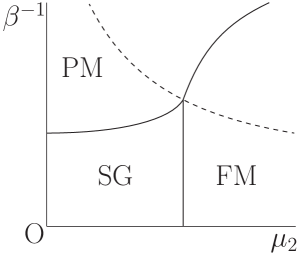
Figure 1: Phase diagram in the Edwards-Anderson model for $p=2$. The ordinate is the temperature $\beta^{-1}$, and the abscissa is the ferromagnetic exchange interaction $\mu_{2}$ between two spins. The solid lines denote the phase boundaries among the ferromagnetic (FM), paramagnetic (PM) and spin glass (SG) phases. The broken line denotes the Nishimori line. Theorem 2.2 implies that sample expectation of the spontaneous magnetization does not exist. This fact guarantees that the phase boundary between spin glass and ferromagnetic phases is conjectured to be vertical [33]. Reproduced with permission from [33].

Theorem 2.6 concludes the absence of RSB on the Nishimori line in a rigorous manner. Identities given by Nishimori’s gauge theory combined with the ACGG identities [1, 12, 13, 16, 17, 18, 19, 26, 28, 29, 41] enable us to prove that variances of the magnetization and the spin overlap vanish on the Nishimori line. Nishimori and Sherrington obtained the same result [35] by showing that the distribution function of the spin overlap is identical to that of the magnetization on the Nishimori line. Their result for the overlap depends on the assumption that the distribution of the magnetization is concentrated at a single value on the Nishimori line. We have proven this concentration property of the magnetization and the spin overlap in the same way to obtain the ACGG identities.

Acknowledgments

C.I. is supported by JSPS (21K03393).

There is no conflict of interest. All data are provided in full in this paper.

References

• [1] Aizenman, M. and Contucci, P. :On the stability of quenched state in mean-field spin glass models. J. Stat. Phys. 92, 765-783 (1997)
• [2] Aizenman, M., Greenblatt, R. L. and Lebowitz, J. L. :Proof of rounding by quenched disorder of first order transitions in low-dimensional quantum systems. J. Math. Phys. 53, 023301 (2012)
• [3] Aizenman, M. and Wehr, J. :Rounding effects of quenched randomness on first-order phase transitions. Commun. Math. Phys. 130, 489-528 (1990)
• [4] Agliari, E., Barra, A., Burioni, R. and Di Biasio, A. : Notes on the p-spin glass studied via Hamilton-Jacobi and smooth-cavity techniques. J. Math. Phys. 53, 063304 (2012)
• [5] Agliari, E., Fachechi, A. and Marullo, C. : Nonlinear PDEs approach to statistical mechanics of dense associative memories. J. Math. Phys. 63, 103304 (2022)
• [6] Albanese, L. and Alessandrelli, A. : Rigorous approaches for spin glass and Gaussian spin glass with P-wise interactions. preprint, arXiv:2111.12569 (2021)
• [7] Alberici, D., Camilli, F., Contucci, P. and Mingione, E. : The multi-species mean-field spin-glass on the Nishimori line. J. Stat. Phys. 182, 2 (2021)
• [8] Barra, A., Di Biasio, A. and Guerra, F. : Replica symmetry breaking in mean-field spin glasses through the Hamiltonian-Jacobi technique. J. Stat. Mech. P09006 (2010)
• [9] Barra, A., Dal Ferraro, G. and Tantari, D. : Mean field spin glasses treated with PDE techniques. Eur. Phys. J. B 86, 332 (2013)
• [10] Barbier, J., Dia, M., Macris, N., Krzakala, F., Lesieur, T. and ZdeborovΓ‘, L. : Mutual information for symmetric rank-one matrix estimation: A proof of the replica formula. Advances in Neural Information Processing Systems 29, 424-432 (2016)
• [11] Barbier, J., Dia, M., Macris, N., Krzakala, F. and ZdeborovΓ‘, L. : Rank-one matrix estimation: analysis of algorithmic and information theoretic limits by the spatial coupling method. preprint, arXiv:1812.02537 (2018)
• [12] Chatterjee, S. :The Ghirlanda-Guerra identities without averaging. preprint, arXiv:0911.4520 (2009).
• [13] Chatterjee, S. :Absence of replica-symmetry breaking in the random field Ising model. Commun. Math .Phys. 337, 93-102 (2015)
• [14] Chen, W-K. :On the mixed even-spin Sherrington-Kirkpatrick model with ferromagnetic interaction. Ann. Henri PoincarΓ© Probab. Stat. 50, 63-83 (2014)
• [15] Chen, W-K. :On the Almeida-Thouless transition line in the Sherrington-Kirkpatrick model with centered Gaussian external field. Electron. Commun. Probab. 26, 65, 1-9 (2021)
• [16] Contucci, P. and GiardinΓ , C. :Spin-glass stochastic stability: A rigorous proof. Ann. Henri Poincare, 6, 915-923 (2005)
• [17] Contucci, P. and GiardinΓ , C. :The Ghirlanda-Guerra identities. J. Stat. Phys. 126, 917-931 (2007)
• [18] Contucci, P. and GiardinΓ , C. :Perspectives on spin glasses. Cambridge university press, 2012.
• [19] Contucci, P., GiardinΓ , C. and Nishimori, H. :Spin glass identities and the Nishimori line. In Spin Glasses: Statics and Dynamics 103-121 Springer, (2009).
• [20] Contucci, P., GiardinΓ , C. and PulΓ©, J. :The infinite volume limit for finite dimensional classical and quantum disordered systems. Rev. Math. Phys. 16, 629-638 (2004)
• [21] Contucci, P. and Lebowitz, J. L. :Correlation inequalities for quantum spin systems with quenched centered disorder. J. Math. Phys. 51, 023302-1 -6 (2010)
• [22] de Almeida, J. R. L. and Thouless, D. J. :Stability of the Sherrington-Kirkpatrick solution of spin glass model. J. Phys. A :Math. Gen. 11, 983-990 (1978)
• [23] Edwards, S. F. and Anderson, P. W. :Theory of spin glasses. J. Phys. F: Metal Phys. 5, 965-974 (1975)
• [24] Guerra, F. :Sum rules for the free energy in the mean field spin glass model. Fields Institute Communications 30, 161-170 (2001)
• [25] Guerra, F. :Broken replica symmetry bounds in the mean field spin glass model. Commun. Math. Phys. 233, 1-12 (2003)
• [26] Ghirlanda, S. and Guerra, F. :General properties of overlap probability distributions in disordered spin systems. Towards Parisi ultrametricity. J. Phys. A:Math. Gen. 31, 9149-9155 (1998)
• [27] Greenblatt, R. L., Aizenman, M. and Lebowitz, J. L. :Rounding first order transitions in low-dimensional quantum systems with quenched disorder. Phys. Rev. Lett. 103, 197201 (2009)
• [28] Itoi, C. :Universal nature of replica-symmetry breaking in disordered quantum systems. J. Stat. Phys. 167, 1262-1279 (2017)
• [29] Itoi, C. :Self-averaging of perturbation Hamiltonian density in perturbed spin systems. J. Stat. Phys. 177, 1063-1076 (2019)
• [30] Itoi, C. and Sakamoto, Y. :Boundedness of Susceptibility in Spin Glass Transition of Transverse Field Mixed $p$-spin Glass Models. J. Phys. Soc. Jpn. 92, 064004 (2023)
• [31] Morita, S., Nishimori, H. and Contucci, P. :Griffiths inequalities for the Gaussian spin glass. J. Phys. A: Math. Gen. 37, L203-211 (2004)
• [32] Morita,S., Ozeki, Y. and Nishimori, H. :Gauge theory for quantum spin glasses. J. Phys. Soc. Jpn. 75, 014001, 1-7 (2006)
• [33] Nishimori, H. :Statistical physics of spin glasses and information processing an introduction. Oxford university press. (2001)
• [34] Nishimori, H. :Internal energy, specific heat and correlation function of the bond-random Ising model. Prog. Theor. Phys. 66, 1169-1181 (1981)
• [35] Nishimori, H. and Sherrington, D. :Absence of replica-symmetry breaking in a region of the phase diagram of the Ising spin glass. AIP conference proceedings 553, 67 (2001)
• [36] Okuyama, M. and Ohzeki, M. :Gibbs-Bogoliubov inequality on Nishimori line. preprint, arXiv:2208.12311 (2022)
• [37] Parisi, G. :Infinite number of order parameters for spin glasses. Phys. Rev. Lett. 43, 1754-1756 (1979).
• [38] Parisi, G. :A sequence of approximate solutions to the S-K model for spin glasses. J. Phys. A: Math. Gen. 13, L115-L121 (1980).
• [39] Sherrington, D. and Kirkpatrick, S. :Solvable model of spin glass. Phys. Rev. Lett. 35, 1792-1796 (1975)
• [40] Talagrand, M. :The Parisi formula. Ann. Math. 163, 221-263 (2006)
• [41] Talagrand, M. :Mean field models for spin glasses. Springer, Berlin (2011)
• [42] Toninelli, F. :About the Almeida-Thouless transition line in the Sherrington-Kirkpatrick mean field spin glass model. Euro. Phys. Lett. 60, 764-767 (2002)