On the Equivalence of Consistency-Type Models: Consistency Models, Consistent Diffusion Models, and Fokker-Planck Regularization

Abstract

The emergence of various notions of “consistency” in diffusion models has garnered considerable attention and helped achieve improved sample quality, likelihood estimation, and accelerated sampling. Although similar concepts have been proposed in the literature, the precise relationships among them remain unclear. In this study, we establish theoretical connections between three recent “consistency” notions designed to enhance diffusion models for distinct objectives. Our insights offer the potential for a more comprehensive and encompassing framework for consistency-type models.

1 Introduction

Score-based generative models (Song & Ermon, 2019; Song et al., 2020b, a; Boffi & Vanden-Eijnden, 2022), commonly referred to as diffusion models (Sohl-Dickstein et al., 2015; Ho et al., 2020), have significantly advanced photorealistic image generation (Saharia et al., 2022; Rombach et al., 2022; Kim et al., 2022) and found applications in diverse domains such as media editing and restoration (Meng et al., 2021; Kawar et al., 2022; Saito et al., 2022; Murata et al., 2023).

Underlying score-based generative model is a (stochastic) differential equation that describes the process of transforming data to noise and vice-versa, which is approximated using a neural (score) network learned from data. Because of the mathematical structure afforded by the underlying differential equation, this neural network needs to satisfy certain consistency properties. Various such notions of consistency have been recently introduced and shown to enhance sample quality (Daras et al., 2023), accelerate sampling speed (Song et al., 2023), and improve likelihood estimation (Lai et al., 2022). We introduce the term consistency-type model to encompass and unify these various concepts. It refers to a (diffusion) model that is explicitly designed to align with the underlying trajectory defined by an ordinary differential equation (ODE), stochastic differential equation (SDE), or partial differential equation (PDE). In this study, we aim to provide a theoretical investigation into the relationships between these three consistency-type models. Under certain mild assumptions, we will rigorously establish the equivalence of these independently developed concepts.

2 Background

Song et al. (2020b) introduced a stochastic differential equation (SDE) framework that unifies the concepts of denoising score matching (Song & Ermon, 2019) and diffusion models (Sohl-Dickstein et al., 2015; Ho et al., 2020) in continuous time. Especially, the process $\{\bm{x}(t)\}_{t\in[0,T]}$ of adding Gaussian noise

$$\bm{x}(t)\sim q_{t}\quad\text{where}\quad q_{t}(\bm{x})=q_{\text{data}}(\bm{x})*\mathcal{N}(\bm{x};\bm{0},\sigma^{2}(t)\bm{I})$$

is driven by the following forward SDE

$$d\bm{x}(t)=g(t)d\bm{w}_{t}.$$ (1)

Here, we define $q_{0}=q_{\text{data}}$, $g(t):=\sqrt{\frac{d\sigma^{2}(t)}{dt}}$, $*$ as the convolution operator, and $\bm{w}_{t}$ as the standard Wiener process. Eq. (1) inherently corresponds to a reverse time SDE from $T$ to $0$ under moderate conditions (Anderson, 1982)

$$d\bm{x}(t)=-g^{2}(t){\nabla_{\bm{\bm{x}}}}\log q_{t}(\bm{x}(t))dt+g(t)d\bar{\bm{w}}_{t},$$ (2)

where $\bar{\bm{w}}_{t}$ is a standard Wiener process in reverse time, and $q_{t}(\bm{x})$ denotes the ground truth marginal density of $\bm{x}(t)$ following Eq. (1).

The stochastic process in Eq. (2) automatically associates with a deterministic process, known as the probability flow (PF) ODE. This PF ODE governs the evolution of samples without any diffusion term and guarantees that the trajectories of the samples maintain identical marginal probability densities as the forward SDE (Eq. (1)). The PF ODE is expressed as follows:

$$\frac{d\bm{x}}{dt}(t)=-\frac{1}{2}g^{2}(t){\nabla_{\bm{\bm{x}}}}\log q_{t}(\bm{x}(t)).$$ (3)

Since $\nabla_{\bm{x}}\log q_{t}(\bm{x}(t))$ is typically unattainable in Eqs. (2) and (3), the denoising score matching (DSM) loss (Vincent, 2011; Song et al., 2020b) is commonly employed to approximate $\nabla_{\bm{x}}\log q_{t}(\bm{x})$ by using a time-conditional neural network $\bm{s}_{\bm{\theta}}=\bm{s}_{\bm{\theta}}(\bm{x},t)$ over the time interval $[t_{0},T]$, where $t_{0}\geq 0$ is chosen to be sufficiently small in practice.

By substituting ${\nabla_{\bm{\bm{x}}}}\log q_{t}(\bm{x})$ with the learned $\bm{s}_{\bm{\theta}}$ in the reverse time SDE described in Eq. (2), and in the PF ODE given by Eq. (9), we obtain parametric counterparts of the reverse time SDE for a stochastic process and the PF PDE for a deterministic process, respectively. Consequently, we have the choice to generate samples by numerically solving either the parametric SDE or the parametric PF PDE in reverse, starting from an initial sample drawn from a predefined prior.

Table 1: Comparison of existing consistency-type models.

Models	Purpose	Trajectory	Object of Eq.	Approach
CDM (Daras et al., 2023)	Sample quality	Backward SDE	Samples	DSM + Martingale regularizer
CM (Song et al., 2023)	Sampling speed	PF ODE	Samples	Specific NN structure + New training scheme
FP-Diffusion (Lai et al., 2022)	Likelihood	Score FPE (a PDE)	Scores	DSM + Score FPE-regularizer

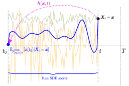
(a) Illustration of Def. 3.1. A consistent SDE-denoiser indicates that the SDE-denoiser prediction $\bm{h}(\bm{x},t)$ (endpoint of the magenta arrow) aligns with the average of SDE predictions $\mathbb{E}_{p_{[t_{0},t],\bm{h}}^{\text{SDE}}}\big{[}\bm{x}(t_{0})|\bm{X}_{t}=\bm{x}\big{]}$ (blue dot).

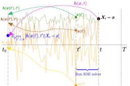
(b) Illustration of Prop. 3.2. The SDE-denoiser prediction $\bm{h}(\bm{x},t)$ (endpoint of the magenta arrow) aligns with the average prediction of intermediate points obtained by first applying an SDE solver and subsequently applying the SDE-denoiser $\mathbb{E}_{p_{[t^{\prime},t],\bm{h}}^{\text{SDE}}}\big{[}\bm{h}(\bm{x}(t^{\prime}),t^{\prime})|\bm{X}_{t}=\bm{x}\big{]}$ (blue dot).

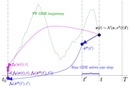
(c) Illustration of Alg. 2 in (Song et al., 2023). The objective of CM is to align the prediction of the direct denoiser (endpoint of the magenta arrow) with the prediction obtained by first applying a one-step ODE solver and subsequently applying the denoiser.

Figure 1: Illustration of a consistent SDE/ODE-denoiser. The dashed curves depict predictions from denoisers. In (a) and (b), the three erratic curves in light hues represent the SDE trajectories; the blue curve in (a) indicates the deterministic trajectory of the average. In (c), the green curve corresponds to the PF ODE trajectory, and $\bm{\phi}$ represents the parameters of a pre-trained score model.

3 Consistency-type models

In this section, we provide an overview of recent literature that incorporates notions of “consistency” in diffusion models. Specifically, we review three notable models: Consistent Diffusion Model (CDM) (Daras et al., 2023), Consistency Model (CM) (Song et al., 2023), and Fokker-Planck (FP) Diffusion (Lai et al., 2022). Table 1 compares the distinguishing characteristics of these consistency-type models.

3.1 CDM (Daras et al., 2023)

Daras et al. (2023) introduced the concept of a “consistent denoiser” for the SDE (2). By leveraging Tweedie’s formula (Efron, 2011), a connection can be established between the score function $\nabla_{\bm{x}}\log q_{t}(\bm{x})$ and a denoiser $\bm{h}\colon\mathbb{R}^{D}\times[t_{0},T]\rightarrow\mathbb{R}^{D}$ conditioned on time

$$\nabla_{\bm{x}}\log q_{t}(\bm{x})=\frac{\bm{h}(\bm{x},t)-\bm{x}}{\sigma^{2}(t)}.$$

Consequently, Eq. (2) can be rearranged as follows:

$$d\bm{x}(t)=-g^{2}(t)\Big{(}\frac{\bm{h}(\bm{x},t)-\bm{x}}{\sigma^{2}(t)}\Big{)}dt+g(t)d\bar{\bm{w}}_{t}.$$ (4)

This reparameterization gives rise to the concept of a consistent denoiser $\bm{h}$ (Daras et al., 2023). A denoiser is considered consistent if, on average, it produces estimates of the nearly clean data that align with those obtained by solving Eq. (4) in reverse, regardless of the initial data used. A concise summary of its formal definition is presented below. Furthermore, Fig. 1(a) showcases its corresponding illustration.

Definition 3.1 (Consistent SDE-denoiser (Daras et al., 2023)).

A function $\bm{h}\colon\mathbb{R}^{D}\times[t_{0},T]\rightarrow\mathbb{R}^{D}$ is called a consistent SDE-denoiser if and only if $\bm{h}(\bm{x},t)=\mathbb{E}_{p_{[t_{0},t],\bm{h}}^{\text{SDE}}}\big{[}\bm{x}(t_{0})|\bm{X}_{t}=\bm{x}\big{]}$ for all $\bm{x}\in\mathbb{R}^{D}$ and $t\in[t_{0},T]$.

Here, $\mathbb{E}_{p_{[t_{0},t],\bm{h}}^{\text{SDE}}}$ denotes the conditional expectation of $\bm{x}(t_{0})$ with respect to the distribution of $p_{[t_{0},t],\bm{h}}^{\text{SDE}}$ along the stochastic trajectory described by the SDE presented in Eq. (4). This trajectory starts with an initial value of $\bm{x}$ at an arbitrary time $t$ and terminates at a generated sample $\bm{x}(t_{0})$ by running the SDE in Eq. (4) backwards in time.

The aim of Daras et al. (2023) is to train a diffusion model to serve as a consistent SDE-denoiser. However, applying this condition to practical settings is challenging due to the time-consuming process outlined in Definition 3.1, which involves multiple SDE solving by running from $t$ to $t_{0}$ in order to accurately evaluate the average. In contrast, Daras et al. (2023) observed that a consistent SDE-denoiser $\bm{h}$ can be interpreted as a reverse martingale under the same process described in Eq. (2). Fig. 1(b) illustrates this property.

Proposition 3.2 (Daras et al. (2023)).

$\bm{h}$ is a consistent SDE-denoiser if and only if the following properties hold:

1. (Reverse martingale) For all $t>t^{\prime}$ and $\bm{x}$, we have $\bm{h}(\bm{x},t)=\mathbb{E}_{p_{[t^{\prime},t],\bm{h}}^{\text{SDE}}}\big{[}\bm{h}(\bm{x}(t^{\prime}),t^{\prime})|\bm{X}_{t}=\bm{x}\big{]}$.

2. (Identity at $t_{0}$) For all $\bm{x}\in\mathbb{R}^{D}$, $\bm{h}(\bm{x},t_{0})=\bm{x}$.

Here, $\mathbb{E}_{p_{[t^{\prime},t],\bm{h}}^{\text{SDE}}}$ represents the conditional expectation of $\bm{x}(t^{\prime})$ given the distribution of $p_{[t^{\prime},t],\bm{h}}^{\text{SDE}}$ along the trajectory described by the SDE in Eq. (4), starting with an initial value $\bm{x}$ at time $t$ and terminates at time $t^{\prime}$.

Based on this proposition, Daras et al. (2023) proposed to train a denoiser $\bm{h}_{\bm{\theta}}$ by using the denoising score matching (DSM) loss, along with a regularizer which is defined as

$$\frac{1}{2}\Big{(}\bm{h}_{\bm{\theta}}(\bm{x},t)-\mathbb{E}_{p_{[t^{\prime},t],\bm{h}_{\bm{\theta}}}^{\text{SDE}}}\big{[}\bm{h}_{\bm{\theta}}(\bm{x}(t^{\prime}),t^{\prime})|\bm{X}_{t}=\bm{x}\big{]}\Big{)}^{2},$$ (5)

and its purpose is to enforce the reverse martingale property. Their approach demonstrates notable improvement in terms of sample quality.

3.2 CM (Song et al., 2023)

Song et al. (2023) directed their attention to PF ODE in Eq. (3) (a deterministic process). They introduced the notion of a “consistency function” which promotes the model’s prediction of nearly clean data that aligns with the trajectory of the PF ODE. In order to establish a better connection with CDM (which will be discussed in Sec. 4.1), we propose a modification to their terminology, replacing “consistency function” with “consistent ODE-denoiser”. Below, we provide the formal definition.

Definition 3.3 (Consistent ODE-denoiser (Song et al., 2023)).

Given a solution trajectory $\{\bm{x}(t)\}_{t\in[t_{0},T]}$ of the PF ODE in Eq. (3). Given a time-dependent vector field $\bm{f}$. $\bm{f}$ is called a consistent ODE-denoiser if it satisfies

$$\bm{f}(\bm{x}(t),t)=\bm{x}(t_{0})\quad\text{for all}\quad t\in[t_{0},T].$$ (6)

A straightforward corollary of the definition is that a consistent ODE-denoiser $\bm{f}$ must fulfill the condition:

$$\bm{f}(\bm{x}(t),t)=\bm{f}(\bm{x}(t^{\prime}),t^{\prime})\quad\text{for all}\quad t,t^{\prime}\in[t_{0},T].$$ (7)

The goal of (Song et al., 2023) is to train a network $\bm{f}_{\bm{\theta}}$ to satisfy both Eqs. (6) and (7). Eq. (6) is guaranteed by employing a specific network design, while Eq. (7) is learned through the minimization of a “distance” measured by $d(\cdot,\cdot)$:

$$d(\bm{f}_{\bm{\theta}}(\bm{x}(t),t),\bm{f}_{\bm{\theta}}(\bm{x}(t^{\prime}),t^{\prime})).$$ (8)

Thanks to the specific design of the network, the learned consistent ODE-denoiser is capable of performing one-step sampling. We visually depict the distillation training of Song et al. (2023) (Algorithm 2) in Fig. 1(c).

3.3 FP-Diffusion (Lai et al., 2022)

Lai et al. (2022) established an equivalent system of PDEs known as the “score Fokker-Planck equation” (score FPE) for the ground truth score (see Eq. (9)), which is built upon the classic FPE introduced by Fokker (1914); Planck (1917). The score FPE describes the temporal evolution of the ground truth score once the forward SDE is given. We present their findings in the following proposition.

Proposition 3.4 (Lai et al. (2022)).

The ground truth score $\bm{s}=\bm{s}(\bm{x},t):=\nabla_{\bm{x}}\log q_{t}(\bm{x})$ satisfies the score FPE

$$\partial_{t}\bm{s} =\frac{1}{2}g^{2}(t){\nabla_{\bm{\bm{x}}}}\big{(}{\textup{div}_{\bm{\bm{x}}}}(\bm{s})+\left\lVert\bm{s}\right\rVert^{2}_{2}\big{)}.$$ (9)

Lai et al. (2022) noted that DSM pre-trained score-based diffusion models often do not conform to the underlying score FPE (which is satisfied by the ground truth score). To address this issue, they proposed a regularization approach by minimizing the residuals of the score FPE, referred to as the score FPE-regularizer, into the DSM loss (as described in Eq. (19) of Lai et al. (2022)). The authors provided both theoretical and numerical evidence that their proposed model, known as FP-Diffusion, can enhance likelihood estimation.

4 Relation of consistency-type models

4.1 CDM and CM

In this section, we establish a connection between CDM and CM. Specifically, we demonstrate that the notion of a consistent SDE-denoiser can be transformed into a consistent ODE-denoiser when the underlying trajectory is governed by a PF ODE.

To rigorously formulate the theorem, we incorporate a parameter $\lambda\geq 0$ that establishes a connection between Eqs. (2) and (3) as Karras et al. (2022)

$$d\bm{x}(t)=-(\frac{1+\lambda}{2})g^{2}(t)\bm{s}(\bm{x},t)dt+\lambda g(t)\bar{\bm{w}}_{t}.$$ (10)

Furthermore, we introduce $\mathbb{E}_{p_{[t^{\prime},t],\bm{h}}^{\lambda-\text{SDE}}}$ analogous to Proposition 3.1, to denote the conditional expectation of $\bm{x}(t^{\prime})$ based on the distribution of $p_{[t^{\prime},t],\bm{h}}^{\lambda-\text{SDE}}$ along the stochastic trajectory described by the $\lambda$-parametrized SDE presented in Eq. (10) starting from $\bm{x}(t)$ and terminating at time $t^{\prime}$. It is observed that when $\lambda=1$, Eq. (10) coincides with Eq. (2) and $p_{[t^{\prime},t],\bm{h}}^{1-\text{SDE}}$ is equivalent to $p_{[t_{0},t],\bm{h}}^{\text{SDE}}$. On the other hand, when $\lambda=0$, Eq. (10) becomes the PF ODE in Eq. (3). We now present the relationship of CDM and CM as the following theorem.

Theorem 4.1 (Relationship of CDM and CM).

If $\lambda=0$, then a consistent SDE-denoiser is equivalent to a consistent ODE-denoiser.

Proof.

Consider a denoiser $\bm{h}$ and $\lambda=0$. This is equivalent to the formulation presented in Definition 3.1, but replacing the trajectory governed by the SDE in Eq. (4) with a PF ODE described by Eq.(3). Then for all $t\in[t_{0},T]$, we have $\bm{h}(\bm{x}(t),t)=\mathbb{E}_{p_{[t_{0},t],\bm{h}}^{0-\text{SDE}}}\big{[}\bm{x}(t_{0})|\bm{X}_{t}=\bm{x}(t)\big{]}=\bm{x}(t_{0})$, owing to the deterministic nature of the ODE. Alternatively, we can arrive at the same conclusion by leveraging Proposition 3.2. The reverse martingale property implies that $\bm{h}(\bm{x}(t),t)=\mathbb{E}_{p_{[t^{\prime},t],\bm{h}}^{0-\text{SDE}}}\big{[}\bm{h}(\bm{x}(t^{\prime}),t^{\prime})|\bm{X}_{t}=\bm{x}(t)\big{]}=\bm{h}(\bm{x}(t^{\prime}),t^{\prime})$ holds for all $t^{\prime}<t$, which is a consequence of the ODE trajectory being deterministic. In particular, if we set $t^{\prime}=t_{0}$ and consider condition (ii) of Proposition 3.2, we also obtain $\bm{h}(\bm{x}(t),t)=\bm{h}(\bm{x}(t_{0}),t_{0})=\bm{x}(t_{0})$ for all $t\in[t_{0},T]$. ∎

Both perspectives presented in the proof, namely Definition 3.1 and Proposition 3.2, ultimately yield the same conclusion: the theoretical correlation between Definition 3.1 and Definition 3.3. Indeed, Figs. 1(b) and (c) illustrate an analogy between a consistent SDE-denoiser and ODE-denoiser. Furthermore, it is worth noting that when we incorporate the CDM’s regularizer in Eq. (5) along the PF ODE, it simplifies to $\frac{1}{2}\big{(}\bm{h}_{\bm{\theta}}(\bm{x},t)-\bm{h}_{\bm{\theta}}(\bm{x}(t^{\prime}),t^{\prime})\big{)}^{2}$, which coincides with Eq. (5) when the measurement $d$ is taken as a $\frac{1}{2}$-weighted MSE.

4.2 FP-Diffusion and CDM

According to Daras et al. (2023), a consistent SDE-denoiser $\bm{h}$ is sufficient to guarantee the fulfillment of the score FPE by its corresponding induced score $\bm{s}(\bm{x},t):=\frac{\bm{h}(\bm{x},t)-\bm{x}}{\sigma^{2}(t)}$. In this section, we establish the necessity of this condition, thereby demonstrating the equivalence between these two concepts.

Theorem 4.2 (Equivalence of consistent SDE-denoiser and satisfaction of score FPE).

Let $\bm{h}\colon\mathbb{R}^{D}\times[t_{0},T]\rightarrow\colon\mathbb{R}^{D}$ be a smooth denoiser so that $\bm{h}(\bm{x},t_{0})=\bm{x}$, for all $\bm{x}$. Then $\bm{h}$ is a consistent SDE-denoiser if and only if $\bm{s}$ satisfies Eq. (9).

Proof.

The proof is built upon the approach presented in (Daras et al., 2023). It is important to note that once the forward SDE (Eq. (1)) is defined, it naturally corresponds to a reverse SDE (Eq. (2)). By employing the multidimensional Itô’s Lemma (Daras et al., 2023, Lemma A.2) to Eq. (2), we obtain

$$d\bm{h}=\Big{[}\frac{\partial\bm{h}}{\partial t}-\frac{1}{2}g^{2}(t)\Delta_{\bm{x}}\bm{h}-g^{2}(t)\mathcal{J}_{\bm{h}}\cdot\bm{s}\Big{]}dt+g(t)\mathcal{J}_{\bm{h}}d\bar{\bm{w}}_{t}.$$ (11)

Here $\big{(}\Delta_{\bm{x}}\bm{F}(\bm{x},t)\big{)}_{i}:=\sum_{j=1}^{D}\partial^{2}_{x_{j}}F_{i}(\bm{x},t)$ denotes the $\bm{x}$-Laplacian of a vector field $\bm{F}:=(F_{i})_{i=1}^{D}\colon\mathbb{R}^{D}\times[t_{0},T]\rightarrow\mathbb{R}^{D}$ with a fixed time $t$. Moreover, $\mathcal{J}_{\bm{F}}$ denotes the Jacobian of $\bm{F}$ with respect to $\bm{x}$ (with a fixed time $t$). We know from Proposition 3.2 of Daras et al. (2023) that $\bm{h}$ is a consistent SDE-denoiser if and only if $\bm{h}$ is a reverse martingale. Indeed, it is equivalent to driftlessness of Eq. (11) by applying Proposition A.3. Namely, the following equation is valid

$$\partial_{t}\bm{h}=\frac{1}{2}g^{2}(t)\Delta_{\bm{x}}\bm{h}+g^{2}(t)\mathcal{J}_{\bm{h}}\cdot\bm{s}.$$

Finally, Lemma A.4, establishing a connection between the score FPE and a PDE that a denoiser $\bm{h}$ must satisfy, implies the equivalence of fulfilling the score FPE by $\bm{s}$. ∎

Despite the theoretical equivalence of a consistent SDE-denoiser and the fulfillment of its score FPE, the empirical experiments conducted by Daras et al. (2023) and Lai et al. (2022) used different approaches and achieved different outcomes. Daras et al. (2023) enforced consistency through regularization to promote the martingale property, whereas Lai et al. (2022) applied a regularizer to ensure satisfaction of the score FPE. These different methods result in distinct loss landscapes and optimization dynamics. We defer the empirical investigation of consistency-type models to future research.

5 Conclusion

In this research, we provide a theoretical bridge between different consistency-type models. The results of this study have the potential to inspire the development of a comprehensive framework that ensures consistency and facilitates the simultaneous achievement of several desired benefits, such as accurate likelihood estimation, efficient sampling speed, and high sample quality.

Appendix A Auxiliary lemmas and propositions

In this section, we present essential lemmas for proving Theorem 4.2.

Let us begin by revisiting the definition of a local martingale (Karatzas et al., 1991), which presents a localized version of the martingale property. A stochastic process $\{\bm{X}(t)\}_{t\in[t_{0},T]}$ is considered a local martingale if there exists a sequence of stopping times $\{\tau_{k}\}_{k=1}^{\infty}$ (which are random variables) satisfying the following conditions: (i) $\tau_{k}$ is almost surely increasing, (ii) $\tau_{k}$ diverges to $\infty$ almost surely, and (iii) the stopped process $\bm{X}(\min\{t,\tau_{k}\})$ is a martingale.

It is well-known that a diffusion process without drift (e.g., Eq. (12)) is a local martingale in general. However, it is important to note that without additional conditions, it does not necessarily qualify as a true martingale. Here, we demonstrate a sufficient condition to imply the true martingale property of a local martingale. For the proof of this proposition, we refer to the provided source (Karatzas et al., 1991).

Lemma A.1.

Suppose that $\mathbb{E}\big{[}\int_{t_{0}}^{T}\left\lVert\bm{G}(\bm{X}(\tau),\tau)\right\rVert_{2}^{2}d\tau\big{]}<\infty$. Then the Itô integral defined as

$$\bm{X}(t)=\bm{X}(t_{0})+\int_{t_{0}}^{t}\bm{G}(\bm{X}(\tau),\tau)d\bm{w}_{\tau}$$ (12)

is a martingale.

Next, we present a classic result that establishes the constancy of any continuous local martingale with bounded variation. The proof of this lemma can be found in the reference (Karatzas et al., 1991; Schilling, 2021).

Lemma A.2.

Any continuous local martingale of bounded variation is constant.

Now, we can establish a characterization of the martingale property for solutions of SDEs, which asserts the non-trivial equivalence between a martingale and a “driftless” Itô process.

Proposition A.3.

Assume that a (Itô’s) stochastic process $\{\bm{X}(t)\}_{t\in[t_{0},T]}$ is the strong solution of the following reverse time SDE on $[t_{0},T]$

$$d\bm{X}(t)=\bm{F}(\bm{X}(t),t)dt+\bm{G}(\bm{X}(t),t)d\bar{\bm{w}}_{t}.$$ (13)

Here $\bm{F},\bm{G}\colon\mathbb{R}^{D}\times[t_{0},T]\rightarrow\mathbb{R}^{D}$ are vector fields satisfying some smoothness conditions , and assumed to be Lipschitz and sub-linear. Namely, there is a constant $C>0$ such that

1. (Lipschitzness) For all $\bm{x}$, $\bm{y}\in\mathbb{R}^{D}$ and $t\in[t_{0},T]$

   $$\left\lVert\bm{F}(\bm{x},t)-\bm{F}(\bm{y},t)\right\rVert_{2} +\left\lVert\bm{G}(\bm{x},t)-\bm{G}(\bm{y},t)\right\rVert_{2}\leq C\left\lVert\bm{x}-\bm{y}\right\rVert_{2}.$$

2. (Sub-linearity) For all $\bm{x}\in\mathbb{R}^{D}$ and $t\in[t_{0},T]$

   $$\left\lVert\bm{F}(\bm{x},t)\right\rVert+\left\lVert\bm{G}(\bm{x},t)\right\rVert\leq C(1+\left\lVert\bm{x}\right\rVert_{2}).$$

Then $\bm{X}(t)$ is a reverse martingale if and only if Eq. (13) is driftless, i.e., $\bm{F}\equiv 0$.

The proposition can be understood intuitively by taking expectation of Eq. (13) conditioned on its history $\{\bm{X}(s)\}_{s\leq t}$

$$\frac{d\mathbb{E}[\bm{X}(t)]}{dt}=\mathbb{E}[\bm{F}(\bm{X}(t),t)].$$

$\mathbb{E}[\bm{G}(\bm{X}(t),t)d\bm{w}_{t}]$ is zero because of the zero mean of the standard Wiener process $\bm{w}_{t}$. Therefore, the expectation remains constant (and consequently, independent of the past) if and only if $\bm{F}$ is identically equal to zero. Nevertheless, proving this proposition requires more intricate analysis, and we provide a detailed argument in Appx. B.1.

In the next Lemma, we bridge the score FPE and a PDE that a denoiser $\bm{h}$ should satisfy. To be consistent with notations in (Daras et al., 2023), we can derive the score FPE (Eq. (9)) of the ground truth score $\bm{s}$ as

$$\partial_{t}\bm{s}=\frac{1}{2}g^{2}(t)\Delta_{\bm{x}}\bm{s}+g^{2}(t)\mathcal{J}_{\bm{s}}\cdot\bm{s}.$$ (14)

Here $\big{(}\Delta_{\bm{x}}\bm{F}(\bm{x},t)\big{)}_{i}:=\sum_{j=1}^{D}\partial^{2}_{x_{j}}F_{i}(\bm{x},t)$ denotes the $\bm{x}$-Laplacian of a vector field $\bm{F}:=(F_{i})_{i=1}^{D}\colon\mathbb{R}^{D}\times[t_{0},T]\rightarrow\mathbb{R}^{D}$ with a fixed time $t$. Moreover, $\mathcal{J}_{\bm{F}}$ denotes the Jacobian in $\bm{x}$ of $\bm{F}$ (with a fixed time $t$).

Lemma A.4.

$\bm{s}$ satisfies the score FPE (or equivalently, Eq. (14)) if and only if $\bm{h}$ satisfies

$$\partial_{t}\bm{h}=\frac{1}{2}g^{2}(t)\Delta_{\bm{x}}\bm{h}+g^{2}(t)\mathcal{J}_{\bm{h}}\cdot\bm{s}.$$ (15)

Appendix B Proofs

B.1 Proof of Proposition. A.3

Proof.

We establish the case for forward time SDEs and martingales, as the reverse time case can be derived through a similar line of reasoning (Klenke, 2013). We first prove the sufficient implication. Suppose that $\bm{X}(t)$ is a martingale. Then the Itô process $\bm{U}(t)$ defined as

$$\bm{U}(t):= \int_{t_{0}}^{t}\bm{F}(\bm{X}(\tau),\tau)d\tau$$

$$= ~{}\bm{X}(t)-\bm{X}(t_{0})-\int_{t_{0}}^{t}\bm{G}(\bm{X}(\tau),\tau)d\bm{w}_{\tau}$$

is a local martingale by the preservation of the local martingale property. It can be observed that $\bm{U}(t)$ possesses a continuous path and bounded variation on the interval $[t_{0},T]$, as a result of property (i) and the assumed smoothness. By utilizing Lemma A.2, we conclude that $U(t)$ is constant, specifically zero. Consequently, Eq. (13) is driftless.

Next, we prove the necessity. Suppose that $\bm{F}\equiv 0$. Thanks to conditions (i) and (ii) (and some additional technical conditions), the existence and uniqueness of the solution to Eq. (13) is guaranteed (see in (Øksendal, 2003, Theorem 5.2.1)) and the solution is finite in the $L_{2}$-sense

$$\mathbb{E}\big{[}\int_{t_{0}}^{T}\left\lVert X(\tau)\right\rVert_{2}^{2}d\tau\big{]}<\infty.$$

We will show that it implies $\mathbb{E}\big{[}\int_{t_{0}}^{T}\left\lVert\bm{G}(\bm{X}(\tau),\tau)\right\rVert_{2}^{2}d\tau\big{]}<\infty$. Consequently, according to Lemma A.1, it guarantees that $\bm{X}$ is a martingale. The sub-linearity of $\bm{G}$ indicates

$$\left\lVert\bm{G}(\bm{x},t)\right\rVert_{2}^{2}\leq C^{2}(1+\left\lVert x\right\rVert_{2})^{2}\leq 2C^{2}(1+\left\lVert x\right\rVert_{2}^{2}).$$

So

$$\mathbb{E}\big{[}\int_{t_{0}}^{T}\left\lVert\bm{G}(\bm{X}(\tau),\tau)\right\rVert_{2}^{2}d\tau\big{]}\lesssim(T-t_{0})+\mathbb{E}\big{[}\int_{t_{0}}^{T}\left\lVert\bm{X}(\tau)\right\rVert_{2}^{2}d\tau\big{]}<\infty.$$

Here we use $\lesssim$ to absorb multiplicative constants. Consequently, utilizing Lemma A.1 and relying on the uniqueness of the strong solution, it follows that $\bm{X}$ is a martingale. ∎

B.2 Proof of Lemma. A.4

Proof.

Suppose that $\bm{s}$ satisfies Eq. (14). We know that $\bm{h}(\bm{x},t)=\bm{x}+\sigma^{2}(t)\bm{s}(\bm{x},t)$. By taking $\partial_{t}$ and using the chain rule, we obtain

$$\begin{aligned} \partial_{t}\bm{h}&=\frac{d\sigma^{2}(t)}{dt}\bm{s}+\sigma^{2}(t)\partial_{t}\bm{s}\\ &=g^{2}(t)\bm{s}+\sigma^{2}(t)\Big{(}\frac{1}{2}g^{2}(t)\Delta_{\bm{x}}\bm{s}+g^{2}(t)\mathcal{J}_{\bm{s}}\cdot\bm{s}\Big{)}.\end{aligned}$$ (16)

Notice that $\Delta_{\bm{x}}\bm{s}(\bm{x},t)=\Delta_{\bm{x}}\big{(}\frac{\bm{h}(\bm{x},t)-\bm{x}}{\sigma^{2}(t)}\big{)}=\frac{1}{\sigma^{2}(t)}\Delta_{\bm{x}}\bm{h}(\bm{x},t)$ and that $\mathcal{J}_{\bm{s}}=\frac{1}{\sigma^{2}(t)}(\mathcal{J}_{\bm{h}}-\bm{I})$, where $\bm{I}$ denote the identity matrix on $\mathbb{R}^{D}$. So Eq. (16) becomes

$$\begin{aligned} \partial_{t}\bm{h}&=g^{2}(t)\bm{s}+\frac{1}{2}g^{2}(t)\Delta_{\bm{x}}\bm{h}+g^{2}(t)(\mathcal{J}_{\bm{h}}-\bm{I})\cdot\bm{s}\\ &=\frac{1}{2}g^{2}(t)\Delta_{\bm{x}}\bm{h}+g^{2}(t)\mathcal{J}_{\bm{h}}\cdot\bm{s},\end{aligned}$$

which indicates Eq. (15) is fulfilled by $\bm{h}$. The reverse implication follows with a similar computation. ∎

References

- Anderson (1982) Anderson, B. D. Reverse-time diffusion equation models. Stochastic Processes and their Applications, 12(3):313–326, 1982.
- Boffi & Vanden-Eijnden (2022) Boffi, N. M. and Vanden-Eijnden, E. Probability flow solution of the fokker-planck equation. arXiv preprint arXiv:2206.04642, 2022.
- Daras et al. (2023) Daras, G., Dagan, Y., Dimakis, A. G., and Daskalakis, C. Consistent diffusion models: Mitigating sampling drift by learning to be consistent. arXiv preprint arXiv:2302.09057, 2023.
- Efron (2011) Efron, B. Tweedie’s formula and selection bias. Journal of the American Statistical Association, 106(496):1602–1614, 2011.
- Fokker (1914) Fokker, A. D. Die mittlere energie rotierender elektrischer dipole im strahlungsfeld. Annalen der Physik, 348(5):810–820, 1914.
- Ho et al. (2020) Ho, J., Jain, A., and Abbeel, P. Denoising diffusion probabilistic models. Advances in Neural Information Processing Systems, 33:6840–6851, 2020.
- Karatzas et al. (1991) Karatzas, I., Karatzas, I., Shreve, S., and Shreve, S. E. Brownian motion and stochastic calculus, volume 113. Springer Science & Business Media, 1991.
- Karras et al. (2022) Karras, T., Aittala, M., Aila, T., and Laine, S. Elucidating the design space of diffusion-based generative models. arXiv preprint arXiv:2206.00364, 2022.
- Kawar et al. (2022) Kawar, B., Elad, M., Ermon, S., and Song, J. Denoising diffusion restoration models. arXiv preprint arXiv:2201.11793, 2022.
- Kim et al. (2022) Kim, D., Kim, Y., Kang, W., and Moon, I.-C. Refining generative process with discriminator guidance in score-based diffusion models. arXiv preprint arXiv:2211.17091, 2022.
- Klenke (2013) Klenke, A. Probability theory: a comprehensive course. Springer Science & Business Media, 2013.
- Lai et al. (2022) Lai, C.-H., Takida, Y., Murata, N., Uesaka, T., Mitsufuji, Y., and Ermon, S. Improving score-based diffusion models by enforcing the underlying score fokker-planck equation. 2022.
- Meng et al. (2021) Meng, C., Song, Y., Song, J., Wu, J., Zhu, J.-Y., and Ermon, S. Sdedit: Image synthesis and editing with stochastic differential equations. arXiv preprint arXiv:2108.01073, 2021.
- Murata et al. (2023) Murata, N., Saito, K., Lai, C.-H., Takida, Y., Uesaka, T., Mitsufuji, Y., and Ermon, S. Gibbsddrm: A partially collapsed gibbs sampler for solving blind inverse problems with denoising diffusion restoration, 2023.
- Øksendal (2003) Øksendal, B. Stochastic differential equations. In Stochastic differential equations, pp. 65–84. Springer, 2003.
- Planck (1917) Planck, V. Über einen satz der statistischen dynamik und seine erweiterung in der quantentheorie. Sitzungberichte der, 1917.
- Rombach et al. (2022) Rombach, R., Blattmann, A., Lorenz, D., Esser, P., and Ommer, B. High-resolution image synthesis with latent diffusion models. In Proceedings of the IEEE/CVF Conference on Computer Vision and Pattern Recognition, pp. 10684–10695, 2022.
- Saharia et al. (2022) Saharia, C., Chan, W., Saxena, S., Li, L., Whang, J., Denton, E., Ghasemipour, S. K. S., Ayan, B. K., Mahdavi, S. S., Lopes, R. G., et al. Photorealistic text-to-image diffusion models with deep language understanding. arXiv preprint arXiv:2205.11487, 2022.
- Saito et al. (2022) Saito, K., Murata, N., Uesaka, T., Lai, C.-H., Takida, Y., Fukui, T., and Mitsufuji, Y. Unsupervised vocal dereverberation with diffusion-based generative models. arXiv preprint arXiv:2211.04124, 2022.
- Schilling (2021) Schilling, R. L. Brownian Motion: A Guide to Random Processes and Stochastic Calculus. Walter de Gruyter GmbH & Co KG, 2021.
- Sohl-Dickstein et al. (2015) Sohl-Dickstein, J., Weiss, E., Maheswaranathan, N., and Ganguli, S. Deep unsupervised learning using nonequilibrium thermodynamics. In International Conference on Machine Learning, pp. 2256–2265. PMLR, 2015.
- Song & Ermon (2019) Song, Y. and Ermon, S. Generative modeling by estimating gradients of the data distribution. Advances in Neural Information Processing Systems, 32, 2019.
- Song et al. (2020a) Song, Y., Garg, S., Shi, J., and Ermon, S. Sliced score matching: A scalable approach to density and score estimation. In Uncertainty in Artificial Intelligence, pp. 574–584. PMLR, 2020a.
- Song et al. (2020b) Song, Y., Sohl-Dickstein, J., Kingma, D. P., Kumar, A., Ermon, S., and Poole, B. Score-based generative modeling through stochastic differential equations. arXiv preprint arXiv:2011.13456, 2020b.
- Song et al. (2023) Song, Y., Dhariwal, P., Chen, M., and Sutskever, I. Consistency models. arXiv preprint arXiv:2303.01469, 2023.
- Vincent (2011) Vincent, P. A connection between score matching and denoising autoencoders. Neural computation, 23(7):1661–1674, 2011.