The Belle II Collaboration

Precise measurement of the $D^{+}_{s}$ lifetime at Belle II

Abstract

We measure the lifetime of the $D_{s}^{+}$ meson using a data sample of 207 fb^-1 collected by the Belle II experiment running at the SuperKEKB asymmetric-energy $e^{+}e^{-}$ collider. The lifetime is determined by fitting the decay-time distribution of a sample of $116\times 10^{3}$ $D_{s}^{+}\!\rightarrow\!\phi\pi^{+}$ decays. Our result is $\tau_{D^{+}_{s}}=(499.5\pm 1.7\,\pm 0.9)$ fs, where the first uncertainty is statistical and the second is systematic. This result is significantly more precise than previous measurements.

The lifetime of a particle, like its mass and spin, is one of the fundamental properties that distinguishes it from other particles. The lifetime is the reciprocal of the total decay width, which is the sum of all partial decay widths. Each partial width is proportional to the magnitude squared of the sum of all decay amplitudes to a final state, and thus every decay amplitude potentially affects the lifetime. As a result, the lifetime can provide information about amplitudes that are difficult to measure or calculate.

Lifetimes of $D$ mesons are dominated by partial widths to hadronic final states. The relatively long lifetime of the $D^{+}$ meson, 2.5 times that of the $D^{0}$, implies there is a reduction in hadronic partial widths. This reduction is attributed to destructive interference between a “spectator” amplitude and a color-suppressed amplitude (Fig. 1, left) [1]. The small difference in lifetimes of the $D^{0}$ and $D^{+}_{s}$ mesons is attributed to the dominance of the spectator amplitude for hadronic decays and different color factors that enter subdominant “exchange” ($D^{0}$) and “annihilation” ($D^{+}_{s}$) amplitudes [2]. The latter amplitude for $D^{+}_{s}$ decays (Fig. 1, right) is Cabibbo-favored and thus plays a larger role than it does for $D^{+}$ decays, in which it is Cabibbo-suppressed.

Figure 1: Left: spectator amplitude (top) and color-suppressed amplitude (bottom). Right: annihilation amplitude.

Hadron lifetimes are difficult to calculate theoretically, as they depend on nonperturbative effects arising from quantum chromodynamics (QCD). Thus, lifetime calculations are performed using phenomenological methods such as the heavy quark expansion [3, 4, 5, 6, 7, 8]. Comparing calculated values with measured values improves our understanding of QCD, which leads to improved QCD calculations of other quantities such as hadron masses, structure functions, etc. [9]. Measurements of the $D_{s}^{+}$ lifetime have been reported by many experiments [10, 11, 12, 13, 14, 15, 16]; the world average value is $\tau_{D^{+}_{s}}=(504\pm 4)$ fs [17]. In this Letter, we present a new measurement of the $D^{+}_{s}$ lifetime using $D^{+}_{s}\!\rightarrow\!\phi\pi^{+}$ decays [18] reconstructed in 207 fb^-1 of data collected by the Belle II experiment [19, 20]. The data were recorded at an $e^{+}e^{-}$ center-of-mass energy corresponding to the $\Upsilon(4S)$ resonance, and at an energy slightly below. Our result has significantly greater precision than the world average value.

The Belle II experiment runs at the SuperKEKB $e^{+}e^{-}$ collider [21]. The overall detector [19] has a cylindrical geometry and includes a two-layer silicon-pixel detector (PXD) surrounded by a four-layer double-sided silicon-strip detector (SVD) [22] and a 56-layer central drift chamber (CDC). These detectors reconstruct tracks (trajectories of charged particles). Only one sixth of the second layer of the PXD was installed for the data analyzed here. The axis of symmetry of these detectors, defined as the $z$ axis, is almost coincident with the direction of the electron beam. Surrounding the CDC is a time-of-propagation counter (TOP) [23] in the central region, and an aerogel-based ring-imaging Cherenkov counter (ARICH) in the forward region. These detectors provide charged-particle identification. Surrounding the TOP and ARICH is an electromagnetic calorimeter based on CsI(Tl) crystals that provides energy and timing measurements for photons and electrons. Outside of the calorimeter is an iron flux return for a superconducting solenoid magnet. The flux return is instrumented with resistive plate chambers and plastic scintillator modules to detect muons, $K^{0}_{L}$ mesons, and neutrons. The solenoid magnet provides a 1.5 T magnetic field that is parallel to the $z$ axis.

We use Monte Carlo (MC) simulated events to optimize event selection criteria, calculate reconstruction efficiencies, and study sources of background. We generate $e^{+}e^{-}\!\rightarrow\!q\bar{q}~{}(q=u,d,s,c,b)$ events using the KKMC package [24] and simulate quark hadronization using the Pythia 8 package [25]. Hadron decays are simulated using EvtGen [26], and the detector response is simulated using Geant4 [27]. Final-state radiation is included in the simulation via Photos [28]. Both MC-simulated events and collision data are reconstructed using the Belle II analysis software framework [29, 30]. To avoid introducing bias in our analysis, we analyze the data in a “blind” manner, i.e, we finalize all selection criteria and the fitting procedure before evaluating the lifetime of signal candidates.

We reconstruct $D^{+}_{s}\!\rightarrow\!\phi\pi^{+}$ decays by first reconstructing $\phi\!\rightarrow\!K^{+}K^{-}$ decays and subsequently pairing the $\phi$ candidate with a $\pi^{+}$ track. We select well-measured tracks by requiring that each track have at least one hit (measured point) in the PXD, four hits in the SVD, and 30 hits in the CDC. We select tracks that originate from near the interaction point (IP) by requiring $|\delta z|<2.0$ cm and $\delta r<0.5$ cm, where $\delta z$ is the displacement of the track from the IP along the $z$ axis, and $\delta r$ is the radial displacement in the plane transverse to the $z$ axis. The IP position is measured at regular intervals of data-taking using $e^{+}e^{-}\!\rightarrow\!\mu^{+}\mu^{-}$ events. The spread of the IP position is typically $250~{}\mu$m in the $z$ direction, $10~{}\mu$m in the transverse horizontal direction ($x$), and only $0.3$ $\mu$m in the transverse vertical direction ($y$). We have checked that none of the above requirements, nor any subsequent selection requirements, bias the lifetime measurement.

We identify tracks as pions or kaons based on Cherenkov light recorded in the TOP and ARICH, and specific ionization ($dE/dx$) information from the CDC and SVD. This information is combined to calculate a likelihood ${\cal L}_{K,\pi}$ for a track to be a $K^{+}$ or $\pi^{+}$. Tracks having a ratio ${\cal L}_{K}/({\cal L}_{K}+{\cal L}_{\pi})>0.60$ are identified as kaon candidates, while tracks having ${\cal L}_{K}/({\cal L}_{K}+{\cal L}_{\pi})<0.55$ are identified as pion candidates. These requirements are 90% and 95% efficient for kaons and pions, respectively.

To reconstruct $\phi\!\rightarrow\!K^{+}K^{-}$ decays, we combine two kaon candidate tracks having opposite charge and an invariant mass satisfying $1.010~{}{\rm GeV}/c^{2}<M(K^{+}K^{-})<1.030~{}{\rm GeV}/c^{2}$. This selected range retains 91% of $\phi\!\rightarrow\!K^{+}K^{-}$ decays. We pair $\phi$ candidates with $\pi^{+}$ tracks to form $D_{s}^{+}$ candidates and require that the invariant mass satisfy a loose requirement of $1.922~{}{\rm GeV}/c^{2}<M(\phi\pi^{+})<2.020~{}{\rm GeV}/c^{2}$. We fit the three tracks to a common vertex using the TreeFitter algorithm [31]. The vertex position resulting from the fit is taken as the decay vertex of the $D_{s}^{+}$. The fit includes a constraint that the $D_{s}^{+}$ trajectory be consistent with originating from the IP; this constraint improves the resolution on the $D_{s}^{+}$ decay time by a factor of three.

To eliminate $D_{s}^{+}$ mesons originating from $B$ decays, which would not have a properly determined decay time, we require that the momentum of the $D_{s}^{+}$ in the $e^{+}e^{-}$ center-of-mass frame be greater than 2.5 GeV/$c$. This selection eliminates all $D_{s}^{+}$ mesons from $B$ decays while retaining 67% of those produced via $e^{+}e^{-}\!\rightarrow\!c\bar{c}$. We reduce background arising from random combinations of $\phi$ and $\pi^{+}$ candidates by requiring $|\cos\theta_{K}|>0.45$, where $\theta_{K}$ is the angle in the $\phi$ rest frame between the $K^{-}$ momentum and the direction of the $D_{s}^{+}$. This requirement reduces combinatorial background by 40% while retaining 90% of signal decays. After applying all selection criteria, about 2% of events have more than one $D^{+}_{s}\!\rightarrow\!\phi\pi^{+}$ candidate. False signal candidates arise mainly from combinations of $\phi$ decays with unrelated $\pi^{+}$ tracks. These do not peak in $M(\phi\pi^{+})$ and are counted as background in our fits for signal yield and $D_{s}^{+}$ lifetime; consequently, they have a negligible effect on the fitted lifetime. We thus retain all signal candidates.

The final $M(\phi\pi^{+})$ distribution is shown in Fig. 2. We perform an unbinned maximum likelihood fit to $M(\phi\pi^{+})$ to determine the yield of $D^{+}_{s}\!\rightarrow\!\phi\pi^{+}$ decays. The signal shape is modeled as the sum of two Gaussian functions and an asymmetric Student’s t distribution. The background contains no peaking structure ($>\!95\%$ consists of random combinations of $\phi$ and $\pi^{+}$ candidates) and is well-modeled by a second-order polynomial. To measure the $D_{s}^{+}$ lifetime, we select candidates having an invariant mass satisfying $1.960~{}{\rm GeV}/c^{2}<M(\phi\pi^{+})<1.976~{}{\rm GeV}/c^{2}$. This range retains 95% of $D^{+}_{s}\!\rightarrow\!\phi\pi^{+}$ decays. In this signal region, the fit yields 115560 signal decays and 9970 background events; the signal purity (ratio of signal over the total) is 92%.

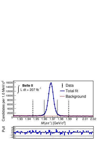
Figure 2: Distribution of $M(\phi\pi^{+})$ for $D^{+}_{s}\!\rightarrow\!\phi\pi^{+}$ candidates, with the fit result overlaid. Black dots correspond to the data; the red dashed curve shows the background component; and the blue solid curve shows the overall fit result. Vertical dotted lines denote the signal region, and vertical dot-dashed lines denote the upper and lower boundaries of the lower and upper sidebands (see text). The corresponding pull distribution is shown in the lower panel, where the pull is defined as $({\rm data}-{\rm fit})/({\rm statistical\ uncertainty\ in\ data})$.

The decay time of a $D_{s}^{+}$ candidate is calculated as

$$t = \left(\frac{\vec{d}\cdot\vec{p}}{p^{2}}\right)m_{D_{s}^{+}}\,,$$ (1)

where $\vec{d}$ is the displacement vector from the IP to the $D_{s}^{+}$ decay vertex, $\vec{p}$ is the $D_{s}^{+}$ momentum, and $m_{D_{s}^{+}}$ is the known $D_{s}^{+}$ mass [17]. The average resolution on $t$ is 108 fs. We determine the $D^{+}_{s}$ lifetime by performing an unbinned maximum likelihood fit to two observables: the decay time $t$ and the per-candidate uncertainty on $t$ ($\sigma_{t}$) as calculated from the uncertainties on $\vec{d}$ and $\vec{p}$. The likelihood function for the $i$th candidate is given by

$${\cal L}(\tau|t^{i},\sigma_{t}\!\!{}^{i}) = f_{\rm sig}\,P_{\rm{sig}}(t^{i}|\tau,\sigma_{t}\!\!{}^{i})\,P_{\rm{sig}}(\sigma_{t}\!\!{}^{i})\ +\$$ (2)

$$\hskip 5.78172pt(1-f_{\rm{sig}})\,P_{\rm{bkg}}(t^{i}|\sigma_{t}\!\!{}^{i})\,P_{\rm{bkg}}(\sigma_{t}\!\!{}^{i}),$$

where $f_{\rm sig}$ is the fraction of events that are signal $D^{+}_{s}\!\rightarrow\!\phi\pi^{+}$ decays; $P_{\rm sig}(t|\tau,\,\sigma_{t})$ and $P_{\rm bkg}(t|\sigma_{t})$ are probability density functions (PDFs) for signal and background events for a reconstructed decay time $t$, given a $D^{+}_{s}$ lifetime $\tau$ for signal and an uncertainty $\sigma_{t}$; and $P_{\rm sig}(\sigma_{t})$ and $P_{\rm bkg}(\sigma_{t})$ are the respective PDFs for $\sigma_{t}$. To reduce highly mismeasured events that are difficult to simulate, we impose loose requirements $-2000~{}{\rm fs}<t<4000$ fs and $\sigma_{t}<900$ fs. These requirements reject less than 0.1% of signal candidates.

The signal PDF is the convolution of an exponential function and a resolution function $R$:

$$P_{\rm sig}(t^{i}|\tau,\sigma_{t}\!\!{}^{i}) = \frac{1}{\tau}\int e^{-t^{\prime}/\tau}\,R(t^{i}-t^{\prime};\mu,s,\sigma_{t}\!\!{}^{i})\,dt^{\prime},$$ (3)

where $R(t^{i}-t^{\prime};\mu,s,\sigma_{t}\!\!{}^{i})$ is a single Gaussian function with mean $\mu$ and a per-candidate standard deviation $s\times\sigma_{t}\!\!{}^{i}$. The scaling factor $s$ accounts for under- or over-estimation of the uncertainty $\sigma_{t}\!\!{}^{i}$. The PDF $P_{\rm bkg}(t\,|\sigma_{t})$ is determined by fitting the decay-time distribution of events in the $M(\phi\pi^{+})$ “upper” sideband $1.990~{}{\rm GeV}/c^{2}<M(\phi\pi^{+})<2.020~{}{\rm GeV}/c^{2}$, which has no contamination from signal decays with final-state radiation. We model $P_{\rm bkg}(t|\sigma_{t})$ as the sum of three asymmetric Gaussians with a common mean. We use MC simulation to verify that the decay-time distribution of background events in this sideband describes well the decay-time distribution of background events in the signal region.

The PDFs $P_{\rm sig}(\sigma_{t})$ and $P_{\rm bkg}(\sigma_{t})$ are taken to be finely binned histograms. The former is determined from the $\sigma_{t}$ distribution of events in the signal region, after subtracting the $\sigma_{t}$ distribution of events in the $M(\phi\pi^{+})$ sideband. The resulting $P_{\rm sig}(\sigma_{t})$ distribution matches well that of MC-simulated signal decays. The $P_{\rm bkg}(\sigma_{t})$ distribution is determined from background events in the $M(\phi\pi^{+})$ sideband. The signal fraction $f_{\rm{sig}}$ is obtained from the earlier fit to the $M(\phi\pi^{+})$ distribution (Fig. 2) and fixed in this fit. Thus, there are three floated parameters: the lifetime $\tau$, and the mean parameter $\mu$ and scaling factor $s$ of the resolution function. These are determined by maximizing the total log-likelihood $\sum_{i}\ln{\cal L}(\tau|t^{i},\sigma_{t}\!\!{}^{i})$, where the sum runs over all events in the signal region.

The result of the fit is $\tau=498.70\pm 1.71$ fs, where the uncertainty is statistical only. The projection of the fit for $t$ is shown in Fig. 3 along with the resulting pulls; the $\chi^{2}$ divided by the number of degrees of freedom ($100-4=96$) is 1.02. The values $\mu=0.56\pm 0.86$ fs and $s=1.22\pm 0.01$ obtained for the resolution function are similar to those obtained from MC-simulated samples.

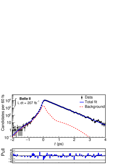
Figure 3: Distribution of $t$ for $D^{+}_{s}\!\rightarrow\!\phi\pi^{+}$ candidates, with the fit result overlaid. Black dots correspond to the data; the red dashed curve shows the background component; and the blue solid curve shows the overall fit result. The corresponding pull distribution is shown in the lower panel.

The main systematic uncertainties are listed in Table 1 and evaluated as follows. Uncertainty arising from possible mismodeling of the detector response and possible correlations between $t$ and $\sigma_{t}$ not accounted for by the resolution function is assessed by fitting a large ensemble of MC signal events. The mean of the fitted lifetime values is calculated, and the difference of $-0.85$ fs between the mean value and the input value is used to correct the fitted lifetime. We assign half of this correction as a systematic uncertainty.

There is uncertainty arising from modeling the background decay-time distribution. We model this distribution using background events in the upper $M(\phi\pi^{+})$ sideband $1.990~{}{\rm GeV}/c^{2}<M(\phi\pi^{+})<2.020~{}{\rm GeV}/c^{2}$. To evaluate uncertainty in this model, we choose a lower sideband $1.922~{}{\rm GeV}/c^{2}<M(\phi\pi^{+})<1.946~{}{\rm GeV}/c^{2}$, a combination of the two sidebands, and also the MC-simulated background distribution in the signal region. The largest difference observed between the resulting fitted lifetime and our nominal result is assigned as a systematic uncertainty.

We model both signal and background $\sigma_{t}$ distributions using histogram PDFs, and there is systematic uncertainty arising from our choice for the number of bins (i.e., statistical fluctuations of the sideband data used to obtain the histogram PDF). We evaluate this by changing the number of bins from the nominal value (80) to other values in the range 60–400. For each choice of binning, we refit for $\tau$. The largest difference observed between the resulting values and our nominal value is taken as a systematic uncertainty.

As measuring the decay time depends on a precise determination of the displacement vector $\vec{d}$ and momentum $\vec{p}$ (Eq. 1), there is uncertainty arising from possible misalignments of the PXD, SVD, and CDC detectors. We study the effect of such misalignment using MC events reconstructed with various misalignments. Each sample is equivalent in size to that of the collision data used. The difference between the fitted value of $\tau$ and the result obtained with no misalignment is recorded, and the root-mean-square (r.m.s.) of the distribution of differences is taken as the systematic uncertainty due to possible detector misalignment.

There is uncertainty arising from the fraction of signal candidates ($f_{\rm sig}$), which is fixed in the decay-time fit to the value obtained from the fit to the $M(\phi\pi^{+})$ distribution. We vary this parameter by its uncertainty and take the resulting change in the fitted lifetime as a systematic uncertainty.

There is an uncertainty arising from the global momentum scale of the detector, which is calibrated using the peak position of $D^{0}\!\rightarrow\!K^{-}\pi^{+}$ decays. We evaluate this by varying the global scale factor by its uncertainty ($\pm 0.06\%$) and assigning the resulting variation in the fitted lifetime as a systematic uncertainty.

Finally, we include a systematic uncertainty due to uncertainty in the $D_{s}^{+}$ mass [17], which is used to calculate the decay time from the vectors $\vec{d}$ and $\vec{p}$ [see Eq. (1)]. The total systematic uncertainty is obtained by adding together all individual contributions (listed in Table 1) in quadrature. The result is $\pm 0.87$ fs.

Source	Uncertainty (fs)
Resolution function	$\pm 0.43$
Background $(t,\sigma_{t})$ distribution	$\pm 0.40$
Binning of $\sigma_{t}$ histogram PDF	$\pm 0.10$
Imperfect detector alignment	$\pm 0.56$
Sample purity	$\pm 0.09$
Momentum scale factor	$\pm 0.28$
$D^{+}_{s}$ mass	$\pm 0.02$
Total	$\pm 0.87$

Table 1: Summary of systematic uncertainties.

As a final check of our analysis procedure, we divide the data sample into subsets based on $D_{s}^{+}$ (or $D_{s}^{-}$) charge, $D_{s}^{+}$ momentum, $D_{s}^{+}$ polar angle, $D_{s}^{+}$ azimuthal angle, and data-collection (run) period, and we measure the lifetime separately for each subset. All measured values are consistent with statistical fluctuations about the overall result. The fitted lifetime for different run periods is plotted in Fig. 4.

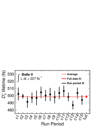
Figure 4: Fitted lifetime for different run periods (c1–c15). For these fits, the parameters of the resolution function are fixed to the overall fitted values. All values are consistent with the overall result, which is plotted as a red data point. The red dashed line shows the average of the lifetime results for the different run periods.

In summary, we have used $116\times 10^{3}$ $D_{s}^{+}\!\rightarrow\!\phi\pi^{+}$ decays reconstructed in 207 fb^-1 of data recorded by Belle II in $e^{+}e^{-}$ collisions at or near the $\Upsilon(4S)$ resonance to measure the $D_{s}^{+}$ lifetime. The result is

$$\tau_{D^{+}_{s}} = (499.5\pm 1.7\,\pm 0.9)~{}{\rm fs,}$$ (4)

where the first uncertainty is statistical and the second is systematic. This is the most precise measurement to date. It is consistent with, but has half the uncertainty of, the current world-average value of $(504\pm 4)$ fs [17]. It is also consistent with theory predictions [3, 6, 8]. The high precision results from significantly improved decay-time resolution as compared to previous $e^{+}e^{-}$ experiments. This is due to the smaller beam sizes of SuperKEKB, which reduce uncertainty on the IP, and to the smaller radius of the first layer of the vertex detector.

This work, based on data collected using the Belle II detector, which was built and commissioned prior to March 2019, was supported by Science Committee of the Republic of Armenia Grant No. 20TTCG-1C010; Australian Research Council and research Grants No. DP200101792, No. DP210101900, No. DP210102831, No. DE220100462, No. LE210100098, and No. LE230100085; Austrian Federal Ministry of Education, Science and Research, Austrian Science Fund No. P 31361-N36 and No. J4625-N, and Horizon 2020 ERC Starting Grant No. 947006 “InterLeptons”; Natural Sciences and Engineering Research Council of Canada, Compute Canada and CANARIE; National Key R&D Program of China under Contract No. 2022YFA1601903, National Natural Science Foundation of China and research Grants No. 11575017, No. 11761141009, No. 11705209, No. 11975076, No. 12135005, No. 12150004, No. 12161141008, and No. 12175041, and Shandong Provincial Natural Science Foundation Project ZR2022JQ02; the Ministry of Education, Youth, and Sports of the Czech Republic under Contract No. LTT17020 and Charles University Grant No. SVV 260448 and the Czech Science Foundation Grant No. 22-18469S; European Research Council, Seventh Framework PIEF-GA-2013-622527, Horizon 2020 ERC-Advanced Grants No. 267104 and No. 884719, Horizon 2020 ERC-Consolidator Grant No. 819127, Horizon 2020 Marie Sklodowska-Curie Grant Agreement No. 700525 ”NIOBE” and No. 101026516, and Horizon 2020 Marie Sklodowska-Curie RISE project JENNIFER2 Grant Agreement No. 822070 (European grants); L’Institut National de Physique Nucléaire et de Physique des Particules (IN2P3) du CNRS (France); BMBF, DFG, HGF, MPG, and AvH Foundation (Germany); Department of Atomic Energy under Project Identification No. RTI 4002 and Department of Science and Technology (India); Israel Science Foundation Grant No. 2476/17, U.S.-Israel Binational Science Foundation Grant No. 2016113, and Israel Ministry of Science Grant No. 3-16543; Istituto Nazionale di Fisica Nucleare and the research grants BELLE2; Japan Society for the Promotion of Science, Grant-in-Aid for Scientific Research Grants No. 16H03968, No. 16H03993, No. 16H06492, No. 16K05323, No. 17H01133, No. 17H05405, No. 18K03621, No. 18H03710, No. 18H05226, No. 19H00682, No. 22H00144, No. 26220706, and No. 26400255, the National Institute of Informatics, and Science Information NETwork 5 (SINET5), and the Ministry of Education, Culture, Sports, Science, and Technology (MEXT) of Japan; National Research Foundation (NRF) of Korea Grants No. 2016R1D1A1B02012900, No. 2018R1A2B3003643, No. 2018R1A6A1A06024970, No. 2018R1D1A1B07047294, No. 2019R1I1A3A01058933, No. 2022R1A2C1003993, and No. RS-2022-00197659, Radiation Science Research Institute, Foreign Large-size Research Facility Application Supporting project, the Global Science Experimental Data Hub Center of the Korea Institute of Science and Technology Information and KREONET/GLORIAD; Universiti Malaya RU grant, Akademi Sains Malaysia, and Ministry of Education Malaysia; Frontiers of Science Program Contracts No. FOINS-296, No. CB-221329, No. CB-236394, No. CB-254409, and No. CB-180023, and No. SEP-CINVESTAV research Grant No. 237 (Mexico); the Polish Ministry of Science and Higher Education and the National Science Center; the Ministry of Science and Higher Education of the Russian Federation, Agreement No. 14.W03.31.0026, and the HSE University Basic Research Program, Moscow; University of Tabuk research Grants No. S-0256-1438 and No. S-0280-1439 (Saudi Arabia); Slovenian Research Agency and research Grants No. J1-9124 and No. P1-0135; Agencia Estatal de Investigacion, Spain Grant No. RYC2020-029875-I and Generalitat Valenciana, Spain Grant No. CIDEGENT/2018/020 Ministry of Science and Technology and research Grants No. MOST106-2112-M-002-005-MY3 and No. MOST107-2119-M-002-035-MY3, and the Ministry of Education (Taiwan); Thailand Center of Excellence in Physics; TUBITAK ULAKBIM (Turkey); National Research Foundation of Ukraine, project No. 2020.02/0257, and Ministry of Education and Science of Ukraine; the U.S. National Science Foundation and research Grants No. PHY-1913789 and No. PHY-2111604, and the U.S. Department of Energy and research Awards No. DE-AC06-76RLO1830, No. DE-SC0007983, No. DE-SC0009824, No. DE-SC0009973, No. DE-SC0010007, No. DE-SC0010073, No. DE-SC0010118, No. DE-SC0010504, No. DE-SC0011784, No. DE-SC0012704, No. DE-SC0019230, No. DE-SC0021274, No. DE-SC0022350, No. DE-SC0023470; and the Vietnam Academy of Science and Technology (VAST) under Grant No. DL0000.05/21-23.

These acknowledgements are not to be interpreted as an endorsement of any statement made by any of our institutes, funding agencies, governments, or their representatives.

References

- Morrison and Witherell [1989] R. J. Morrison and M. S. Witherell, Ann. Rev. Nucl. Part. Sci. 39, 183 (1989).
- Browder et al. [1996] T. E. Browder, K. Honscheid, and D. Pedrini, Ann. Rev. Nucl. Part. Sci. 46, 395 (1996).
- Lenz [2015] A. Lenz, Int. J. Mod. Phys. A 30, 1543005 (2015).
- Neubert [1998] M. Neubert, Adv. Ser. Direct. High Energy Phys. 15, 239 (1998).
- Uraltsev [2000] N. Uraltsev (2000), eprint hep-ph/0010328.
- Lenz and Rauh [2013] A. Lenz and T. Rauh, Phys. Rev. D 88, 034004 (2013).
- Kirk et al. [2017] M. Kirk, A. Lenz, and T. Rauh, JHEP 12, 068 (2017), [Erratum: JHEP 06, 162 (2020)].
- Gratrex et al. [2022] J. Gratrex, B. Melić, and I. Nišandžić, JHEP 07, 058 (2022).
- Aoki et al. [2022] Y. Aoki et al. (Flavour Lattice Averaging Group (FLAG)), Eur. Phys. J. C 82, 869 (2022).
- Aaij et al. [2017] R. Aaij et al. (LHCb Collaboration), Phys. Rev. Lett. 119, 101801 (2017).
- Link et al. [2005] J. M. Link et al. (FOCUS Collaboration), Phys. Rev. Lett. 95, 052003 (2005).
- Iori et al. [2001] M. Iori et al. (SELEX Collaboration), Phys. Lett. B 523, 22 (2001).
- Aitala et al. [1999] E. M. Aitala et al. (E791 Collaboration), Phys. Lett. B 445, 449 (1999).
- Bonvicini et al. [1999] G. Bonvicini et al. (CLEO Collaboration), Phys. Rev. Lett. 82, 4586 (1999).
- Frabetti et al. [1993] P. L. Frabetti et al. (E687 Collaboration), Phys. Rev. Lett. 71, 827 (1993).
- Raab et al. [1988] J. R. Raab et al. (E691 Collaboration), Phys. Rev. D 37, 2391 (1988).
- Workman et al. [2022] R. L. Workman et al. (Particle Data Group), PTEP 2022, 083C01 (2022).
- [18] Throughout this paper, charge-conjugate modes are implicitly included unless noted otherwise.
- Abe [2010] T. Abe (Belle II Collaboration) (2010), eprint arXiv:1011.0352.
- Altmannshofer et al. [2019] W. Altmannshofer et al., PTEP 2019, 123C01 (2019).
- Akai et al. [2018] K. Akai, K. Furukawa, and H. Koiso, Nucl. Instrum. Meth. A907, 188 (2018).
- Adamczyk et al. [2022] K. Adamczyk et al. (Belle II SVD Group), JINST 17, P11042 (2022).
- Wang [2017] B. Wang (Belle II TOP Group) (2017), eprint arXiv:1709.09938.
- Jadach et al. [2000] S. Jadach, B. F. L. Ward, and Z. Wa̧s, Comput. Phys. Commun. 130, 260 (2000).
- Sjöstrand et al. [2015] T. Sjöstrand, S. Ask, J. R. Christiansen, R. Corke, N. Desai, P. Ilten, S. Mrenna, S. Prestel, C. O. Rasmussen, and P. Z. Skands, Comput. Phys. Commun. 191, 159 (2015).
- Lange [2001] D. J. Lange, Nucl. Instrum. Meth. A462, 152 (2001).
- Agostinelli et al. [2003] S. Agostinelli et al. (GEANT4 collaboration), Nucl. Instrum. Meth. A506, 250 (2003).
- Barberio and Was [1994] E. Barberio and Z. Was, Comput. Phys. Commun. 79, 291 (1994).
- Kuhr et al. [2019] T. Kuhr, C. Pulvermacher, M. Ritter, T. Hauth, and N. Braun (Belle II Analysis Software Group), Comput. Softw. Big Sci. 3, 1 (2019).
- [30] https://doi.org/10.5281/zenodo.5574115.
- Krohn et al. [2020] J. F. Krohn et al. (Belle II Analysis Software Group), Nucl. Instrum. Meth. A 976, 164269 (2020).