Sharded Bayesian Additive Regression Trees

Abstract

In this paper we develop the randomized Sharded Bayesian Additive Regression Trees (SBT) model. We introduce a randomization auxiliary variable and a sharding tree to decide partitioning of data, and fit each partition component to a sub-model using Bayesian Additive Regression Tree (BART). By observing that the optimal design of a sharding tree can determine optimal sharding for sub-models on a product space, we introduce an intersection tree structure to completely specify both the sharding and modeling using only tree structures. In addition to experiments, we also derive the theoretical optimal weights for minimizing posterior contractions and prove the worst-case complexity of SBT.

Keywords: Bayesian Additive Regression Trees, model aggregation, optimal experimental design, ensemble model.

1 Background

The motivation of this paper is to improve scalability of regression tree models, and in particular Bayesian (additive) tree models, by introducing a novel model construction where we can adjust the distribute-aggregate paradigm in a flexible way. We consider data with a continuous multivariate input $\bm{x}$, and continuous univariate responses $y$ on the task of regression, however the underlying concepts we introduce are easily generalized to a variety of common scenarios.

1.1 Distributed Markov Chain Monte Carlo

As parallel computation techniques for large datasets become popular in statistics and data science (Pratola et al., 2014; Kontoghiorghes, 2005; Jordan et al., 2019), the problem of distributed inference becomes more important in solving scalability (Jordan et al., 2019; Dobriban and Sheng, 2021). The basic idea of distribute-aggregate inference can be traced back to the bagging technique (Breiman, 1996) for improving model prediction performance. Bayesian modeling can sometimes take model averaging into consideration (Raftery et al., 1997; Wasserman, 2000), by using the distribute-aggregate paradigm for computational scalability on big datasets.

An important example of the distribute-aggregate paradigm arises in Markov chain Monte Carlo (MCMC) sampling for Bayesian modeling, where multiple independent chains could be sampled in parallel, and then combined in some fashion. Distributed inference in MCMC can be introduced as a transition parallel approach, which improves the mixing behavior for modeling with big data (Chowdhury and Jermaine, 2018) using appropriate detailed balance equations. Although transition parallel MCMC can help in general MCMC computations, it does not address the model fitting on big data directly.

Alternatively, to provide computational gains in the big data setting, one is motivated to take a data parallel approach (Scott et al., 2016; Wang and Dunson, 2013) and execute each chain using a subset of the full dataset. Scott et al. (2016) proposed an aggregation approach when the posterior is (a mixture of) Gaussians; and Wang and Dunson (2013) devised a novel sampler to approximate more sophisticated posteriors via Weierstrass transforms.

Our interest lies in Bayesian tree models. Unfortunately, the posterior from Bayesian (additive) tree models belong to neither of these two scenarios and it is unclear how to subset the data and ensure the validity of the aggregated result for tree model posterior distributions.

Echoing the existing literature, our starting point is the consensus Monte Carlo (CMC) algorithm by Scott et al. (2016). CMC proceeds by splitting the full dataset $\mathcal{X}\subset\mathbb{R}^{d}$ consisting of $n$ samples, with inputs $\bm{X}=(\bm{x}_{1}^{T},\cdots,\bm{x}_{n}^{T})^{T},\bm{x}_{1},\cdots,\bm{x}_{n}\in\mathbb{R}^{d}$ and responses $\bm{y}=(y_{1},\cdots,y_{n})^{T}$, into $B$ subsets $\mathcal{X}_{i},\ i=1,\ldots,B,$ each with $n_{i}$ samples ($\sum_{i}^{B}n_{i}=n$), called data shards, such that $\mathcal{X}=\cup_{i=1}^{B}\mathcal{X}_{i}$. The idea of CMC is to distribute each of the $B$ shards across $B$ sub-models distributed to separate compute nodes (i.e., worker machines), and construct $B$ chains for sub-models based on the $\mathcal{X}_{i}$ for each worker machine. Then, one draws Monte Carlo samples for parameters, denoted by $\theta_{j}^{(i)},i=1,2,\cdots,B,j=1,2,\cdots$, from a posterior distribution $p(\theta\mid\mathcal{X}_{i})$ at a much cheaper computational expense as compared to the expense of drawing samples directly from the original posterior $p(\theta\mid\mathcal{X})$.

In this approach, the aggregate posterior sample is taken to be $\theta_{j}=\sum_{i=1}^{B}w_{i}\theta_{j}^{(i)},j=1,2,,\cdots$ where $w_{i}\in[0,1]$ are (static) weights. The parameters $\theta_{j}$’s are considered to be consensus samples drawn from the posterior $p(\theta\mid\mathcal{X})$. These consensus draws represent the consensus belief among all the sub-models’ posterior chains, and when the sharded sub-models and full model posteriors are both Gaussian the weights can be determined to recover the full model’s posterior.

1.2 Scalability of Bayesian Modeling

Scalability issues introduced by either sample size, high dimensionality or intractable likelihoods (Craiu and Levi, 2022), are especially pervasive in the Bayesian context (Wilkinson and Luo, 2022), especially in the Bayesian inference of nonparametric models (Luo et al., 2022; Zhu et al., 2022; Katzfuss and Guinness, 2021; Pratola et al., 2014), which usually require MCMC for model fitting. And while the concept of the CMC inference procedure of Scott et al. (2016) is tempting, it is not obvious how to best select shards, nor how to best aggregate the resulting sharded posteriors, to effectively estimate the original true posterior of interest for sophisticated models.

In other words, precisely how to choose shards $\mathcal{X}_{i}$, and how to appropriately choose the weights $w_{i}$ can be a challenge. This affects the quality of the aggregated model as well as the mixing rates. Compared to the CMC approach, there are at least two additional considerations to contemplate: one is how to select the design and the number of shards to improve the aggregated model prediction, the other is how to weight the sub-models for better posterior convergence and contraction.

The optimality of design can also be crucial in the predictive performance of statistical models (Drovandi et al., 2017; Derezinski et al., 2020; Murray et al., 2023). Usual optimal designs (e.g., Latin hyper-cube) are difficult to elicit (Derezinski et al., 2020), therefore, optimal designs via randomized subsampling are proposed as a computationally efficient alternative (Drovandi et al., 2017). In what follows, we will derive and prove that optimal design for our models is still attainable, conditioned on the shards.

Posterior sampling quality is another important concern. In one initial attempt to apply the distribute-aggregate Monte Carlo scheme in Bayesian modeling, Huggins et al. (2016) focuses on Bayesian logistic regression, and seeks to shard the dataset in such a manner that the sharded likelihoods are “close” to the full-data likelihood in a multiplicative sense. They proposed a single weighted aggregated data subset drawn using multinomial sampling based on weights reflecting the sensitivity of each observation, thereby selecting observations that are “representative” of each cluster of data for each sub-model. Huggins et al. are able to show good performance of their methods, implying that “optimal” selection of shards and weights in CMC could be vital, although a clear connection remained elusive.

Our primary model investigated in this paper, the Bayesian Additive Regression Tree (BART, Chipman et al. (2010)), is additionally constrained by the computationally heavy MCMC procedure used in the posterior sampling of BART. Tree regression models have the natural ability to capture and express interactions of a high-dimensional form without too much smoothness assumptions, while other nonparametric models need explicit terms to capture any assumed interactions. With ensemble constructions such as BART’s sum-of-trees form, tree regressions gain improved predictions and can handle uncertainty quantification. However, as an ensemble method, a tree ensemble also suffers from computational bottlenecks.

We propose a modified BART model that brings the idea of sharding into a cohesive Bayesian model by taking advantange of BART’s tree basis functions. Observing the two sources of computational bottleneck – ensemble and MCMC – the core insight of our proposal builds on that of Bayesian regression trees seen to date: unlike in typical regression where the basis functions are fixed and only the parameters are uncertain, Bayesian regression trees learn both the parameters and the basis functions. In other words, the tree model can serve as basis for and approximate both response and model space.

There are two important assumptions in our distribute-aggregate model : First, we assume that each sub-model is fit using exactly one shard. Second, we assume that the shards are non-intersecting, $\mathcal{X}_{i}\cap\mathcal{X}_{j}=\emptyset$, which can be relaxed in general. These two assumptions simplified our formulations and implementation but are not so restrictive as to limit the applicability of our methods.

In this work, we take a somewhat different perspective on the challenging problem of sharding large datasets in a useful way to perform Bayesian inference. Specifically, while many have focused on methods of approximating a particular posterior distribution, we instead adhere to the notion of including all forms of uncertainty, including data and model uncertainty, into our Bayesian procedure. Since all models are wrong but some are useful (Box, 1976), this seems a more pragmatic and practically useful approach.

Applying this line of thought, our proposed model controls and learns a sharded model space (and relevant model weights) as well as the basis functions and parameters for each model that makes up our collection of models. It is the unique duality of partitions and trees that allows this to be done in a computationally effective manner. The model space is approximated by partitions represented by a tree, whilst the regression basis function and parameters are approximated by functional representation of trees. The idea of learning partitions in a data-driven manner has been explored in previous works on non-parametric modeling (Luo et al., 2021, 2022).

Our approach could recover some reference model of perceived interest if the data warrants it, but practically will recover models which most effectively shard the data thereby allowing faster computation while also providing a better fitting model. Interestingly, our method makes an unexpected connection to the multinomial sampling of Huggins et al. (2016) via an optimal design argument, while using all of the data in a computationally efficient way.

1.3 Organization

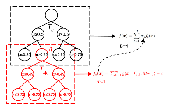
Figure 1: We graphically represent a tree (topology) $\mathcal{T}_{u}$ on the auxiliary variable $\bm{U}$ of depth $k=2$ and $B=4$ leaf nodes whose splitting rules are purely on variable $u$ illustrated in black, and we concatenate another tree (topology, i.e., BART with $m=1$ tree) $\mathcal{T}_{x\mid\eta_{u}}$ illustrated in red, whose root node is the leaf node $\eta=\eta_{u}$ of tree $\mathcal{T}_{u}$, but its splitting rules are purely on input variable $\bm{X}$. We take the convention that $\mathcal{T}_{x\mid\emptyset}$ means the tree only splits on $\bm{X}$.

Our paper proceeds as follows. In Section 2 we review Bayesian tree models, the partitioning interpretation of trees, and develop optimal design results for single-tree models that we will need in our sharded tree model development. In Section 3, we introduce our sharded tree model by using a novel construction involving a latent variable with an optimal sharding tree as described by algorithms; and then we provide some interpretation on the model via notions of weights and marginalization, connecting our construction back to the existing literature. In Section 4 we explore some examples of our proposed model and discuss complexity trade-offs. Finally, we conclude and point out future directions in Section 5.

2 Of Trees and Partitions

2.1 Bayesian Tree Regression Models

Tree models were popularized by the bagging and random forest techniques (Breiman, 1996), and have gained attention in Bayesian forms (Pratola et al., 2020; Chipman et al., 2010; Gramacy and Lee, 2008). Tree models have been shown to be flexible in modeling complex relationships in high-dimensional scenarios. We briefly revisit the Bayesian tree model below, introducing the notations we use, with an emphasis on the tree-induced partition of the input domain.

Example 1.

(Basis functions defined along a path) The general form of a tree $\mathcal{T}$ we will consider in this paper is depicted in Figure 1, which is shown to consist of a subtree splitting on variable $u$, $\mathcal{T}_{u},$ and descendant trees splitting on the input variables $\bm{X}$, shown as $\mathcal{T}_{x|\eta_{u}}.$ We will discuss $\mathcal{T}_{u}$ momentarily, but for now ignore this subtree and simply consider a single tree that only splits on $\bm{X}$, represented as $\mathcal{T}_{x|\emptyset}\equiv\mathcal{T}_{x}$, as shown in Figure 2. Each path in a tree in Figure 2 defines a basis function splitted by the input $\bm{X}$, which is the usual setting in tree models (Wu et al., 2007; Chipman et al., 2010).

Given such a tree $\mathcal{T}_{u}$ consisting of $B$ terminal nodes, each path $\mathcal{P}_{b}$ from terminal node $b$ back to the root node of $\mathcal{T}_{u},$ say $\eta_{1},$ defines a basis function $f_{b}$ that is formed as the product of indicator functions resulting from the evaluation of each internal nodes rule, i.e., the regression function corresponding to this node $b$ can be written as a product of indicator functions where $\mathcal{I}(\cdot;S)$ means the indicator function conditioned on the indicator parameter $S$. For example, the sub-model can be an indicator function along a path $\mathcal{P}_{b}$ in a tree:

$$f_{b}({\bm{x}})=\prod_{\eta_{j}\in\mathcal{P}_{b}}\mathcal{I}\left(\bm{x}_{v_{j}};\rho_{j},c_{j}\right)=\mathcal{I}(\bm{x};R_{b})$$ (1)

where $v_{j}$ is the index of splitting variable of node $\eta_{j}$, $c_{j}$ is the corresponding splitting value and the symbol $\rho_{j}\in\{<,\geq\}$ corresponds to the appropriate inequality sign along the path $\mathcal{P}_{b}$. As we only consider binary trees, then each interior node $\eta_{j}$ can only have a left-child or right-child. The internal structure of $\mathcal{T}_{u}$ can then be fully determined by the collection $\{(v_{j},c_{j})\}$ of splitting indices $v_{j}$ and splitting values $c_{j}$ along with these parent/child relationships.

The important observation here is that the partitioning implied by the product of indicator functions in (1) induces rectangular subregions, the $R_{b}$’s, determined by the given structure of the tree $\mathcal{T}_{x}$. Specifically, each path $\mathcal{P}_{b}$ from the root to a leaf defines a rectangle $R_{b}$, where $\cup_{b=1}^{B}R_{b}=[0,1]^{d}$, for which $f_{b}({\bm{x}})=1$ if ${\bm{x}}\in R_{b}$ and $0$ otherwise.

We model the response $y$ as $f(\bm{x})+\epsilon$ where the conditional mean $\mathbb{E}(y\mid\bm{X}=\bm{x})=f(\bm{x})$ can be written in the following form:

$$f(\bm{x}) =\sum_{b=1}^{B}w_{b}f_{b}(\bm{x}\mid\mu_{b})=\sum_{b=1}^{B}w_{b}f_{b}(\bm{x})$$ (2)

where $w_{b}$ are the weights for single tree models (we can assume $w_{b}=1$ for simplicity now); $\mu_{b}$ is the tree terminal node parameter (as coefficients for sub-models) for terminal node $b$, the noise random variable $\epsilon\sim N(0,\sigma^{2})$ and $f_{b}(\bm{x})$ is an indicator function defined by the rectangle support set $R_{b}$ as defined in (1). Note that this generic tree regression model is conditioned on the tree structure $\mathcal{T}_{x}$.

We denote all the coefficients in (2) as a set $M_{\mathcal{T}_{x}}=\{\mu_{1},\cdots,\mu_{B}\}$. Estimating this regression function in a Bayesian way can be achieved by putting priors on the coefficients $\mu_{b}\in\mathbb{R}$ associated with $\mathcal{T}_{x}$’s leaf nodes $\eta_{x,b}$ and each of these sub-models $f_{b}$. Therefore, (2) can simply be written as $y(\bm{x})=g(\bm{x}\mid\mathcal{T},M_{\mathcal{T}})+\epsilon$ when there is only one tree $\mathcal{T}$.

For a more complex dependence scenario, Chipman et al. (2010) proposed to stack single tree models to obtain BART, where there are $m$ tree regression functions (i.e., number of trees in a BART model) in the regression model:

$$y(\bm{x}) =\sum_{j=1}^{m}g(\bm{x}\mid\mathcal{T}_{x,j},M_{\mathcal{T}_{x,j}})+\epsilon$$ (3)

where $\epsilon\sim N(0,\sigma^{2}).$ Usually, zero mean normal priors are assumed for the coefficients in $M_{\mathcal{T}_{x,k}}$ along with chi-squared variance priors. In what follows, we assume that the noise is known for simplicity, unless otherwise is stated. With (3), it is not hard to see that we are actually creating an ensemble consisting of $B\cdot m$ simple indicator functions.

Our basic and straightforward approach of modifying the BART model (3) is to fit the model using data shards $\mathcal{X}_{1},\cdots,\mathcal{X}_{B}$, where each BART random function $g(\bm{x}|\mathcal{T}_{x,k},M_{\mathcal{T}_{x,k}})$ is fitted using shard $\mathcal{X}_{k}$ (instead of the much larger $\mathcal{X}$) to reduce the computational cost of fitting the model. In this way, the data shards and BART are in one-to-one correspondence so that we fit each shard to a BART model (i.e., $B=2^{\text{depth}}$ in generic weighted model in (2), so $m$ single trees are fitted for each of $B$ leaf nodes):

$$y(\bm{x}) =\sum_{k=1}^{B}\sum_{j=1}^{m}g(\bm{x}\mid\mathcal{T}_{x,j},M_{\mathcal{T}_{x,j}},\mathcal{X}_{k})+\epsilon,$$ (4)

In this approach, within each BART, all $m$ trees share the same data shard.

However, as an alternative of using the same shard across $m$ trees for one BART, we can use different shards across $m$ trees (in fact, the current codebase was most naturally extended in this way, of which (4) is a special case, upon which our theoretical work focuses, for simplicity of exposition). Furthermore, different BART at different leaf nodes do not have to assume the same $m$ but different $m_{1},\cdots,m_{B}$, and different single trees in BART can be fitted on different shards $\mathcal{X}_{k,j}$ instead of using the same $\mathcal{X}_{k}$, namely:

$$y(\bm{x}) =\sum_{k=1}^{B}\sum_{j=1}^{m_{k}}g(\bm{x}\mid\mathcal{T}_{x,j},M_{\mathcal{T}_{x,j}},\mathcal{X}_{k,j})+\epsilon,$$ (5)

and the analysis of this more general form will be left as future work.

The challenge is how to do this in a way that we retain a cohesive estimation and prediction Bayesian model, facilitating both computational efficiency and straightfoward Bayesian inference. Our approach achieves this by recognizing that sharding BART can be induced by representing the data sharding using a tree. To formalize this idea, we examine the equivalence between a tree and a partition next.

2.2 Equivalence between a Tree and a Partition

Our insight begins with recognizing that a tree structure is equivalent to a partition of a metric space (e.g., Talagrand (2022)) as shown in Example 1, which allows us to use the tree to approximate the model space as well as the target function at the same time. However, binary regression trees cannot induce arbitrary partitions. In what follows, we focus on the rectangular partitions that can be induced by regression trees.

The particular partitioning of a dataset could be determined by the construction of a tree structure, in particular its depth, number of terminal nodes, and the selection of splitting points. For balanced trees, we note that any balanced $2^{k}$ partitioning can be represented as a balanced binary tree of depth $k$. Homogeneous partitions can be induced by balanced trees while heterogeneous partitions can be induced by unbalanced trees, as in Figure 2.

Figure 2: A balanced tree of depth $k=2$ and its pruned sub-trees which induced partition on $[0,1]$ (left), and similarly unbalanced trees (middle) and (right). In each of the interior node, we present the splitting rule at $\eta_{j}$ using $\bm{x}_{i,v_{j}}[\rho_{j}]c_{j}$. For simplicity, when the inequality of an interior node holds, we proceed through the left-child node, otherwise we proceed through the right-child node.

2.3 Representing Sharding as a Tree Partition

Now we are ready to take advantage of the partition induced by a tree and use such a partition in creating the data shards in (5). In order to improve the scalability of model fitting through sharding, we will outline a model-based construction to sharding motivated by an optimal design criteria. In this way, we develop a novel tree model that incorporates both modeling and sharding for the input variable $\bm{x}$ in one shot, and we propose to learn the sharding with another tree structure involving an auxilliary random variable $u$.

The sharding created in this way will allow us to attain the distribute-aggregate scheme suggested in Scott et al. (2016) in one unifying model where both the degree of sharding and the sharding weights are informed by the data.

If we take (5) as the regression model, then the sharding on the input $\bm{X}$ cannot be separated from the estimating procedure of $\mathbb{E}\left(y\mid\bm{X}\right)$. To decouple the sharding from the estimation without breaking the model, we observe that the shard partitions can be generated based on an independent random variable $\bm{U}$ while the regression basis functions can be generated based on observations $\bm{X}$. This allows more flexibility in the creation of the partitions, which allocates the observations into different shards, while the regression is still exclusively based on $\bm{X}$. This seemingly straightforward step essentially allows us to present the following regression model with $B$ (the same number as the number of leaves in $\mathcal{T}_{u}$) BART models:

$$y(\bm{x},\bm{u}) =\sum_{k=1}^{B}g_{\text{BART}}(\bm{x}\mid\mathcal{T}_{x\mid\eta,k},M_{\mathcal{T}_{x\mid\eta,k}},\mathcal{T}_{u})+\epsilon.$$ (6)

More precisely, let us introduce the auxiliary vector $\bm{U}=(U_{1},\ldots,U_{n})^{T}$ where each $U_{i}\sim_{iid}\text{Unif}(0,1)$ (or another distribution as illustrated in Appendix A), which is used to augment the observations $\bm{X}$ of size $n$ and define the augmented $n\times(p+1)$ matrix of inputs as $\bm{V}=[\bm{X};\bm{U}].$ We introduce $\bm{u}$ as a device to induce the data shards via a partitioning tree $\mathcal{T}_{u}$ that only splits on this auxiliary variable $\bm{U}$, as depicted in Figure 1. From expression (6), $\mathcal{T}_{u}$ effectively partitions the dataset $\bm{X}$ as well, since the augmented input $\bm{V}=[\bm{X};\bm{U}]$ binds the observed values of $\bm{X}$ and $U$ together. Because the $\bm{X}$ and auxiliary variable $\bm{U}$ are binded, the sample counts can be done on either $\bm{U}$ or $\bm{X}$. As we will see later, the effect of $\bm{U}$ on the posterior of interest can be removed simply by marginalizing it out.

Details of fitting and predicting from our proposed model described by (6) are formalized in Algorithms 1 and 2, and its graphical representation is postponed to Figure 3. For now, we show how the model can be constructed using a tree $\mathcal{T}_{u}$ dedicated to creating data shards, as shown in Figure 8 in Appendix A.

In the rest of the paper, we will focus on the setting where $U\sim\text{Unif}(0,1)$, but point out that there are many possibilities here with different pros and cons, depending on the goal. We focus on one specific sharding tree $\mathcal{T}_{u}$ motivated by an optimal design argument, and show that such a sharding improves posterior concentration rates in the aggregated model.

2.4 Optimal Designs in a Tree

After establishing the basic notations and notions used in our tree models, it is natural to consider what an optimal design (Fedorov, 2013) means for this specific tree model $\mathcal{T}_{u}$ for creating data shards. We will start by considering the optimal design in the fixed location setting (i.e., $\bm{U}$ is deterministic and fixed), then we generalize our discussion to random location setting (i.e., $\bm{U}$ follows a probability distribution $\mathbb{P}$). Considering all terminal node trees $\mathcal{T}_{x\mid\eta_{u}}$ to have only root node for the moment, we focus on the design of $\mathcal{T}_{u}$. This setting is conditionally equivalent to the following generic linear regression model for the data with inputs $\bm{u}\in\mathbb{R}^{d}$ and response $y\in\mathbb{R}^{1}$ as follows:

$$y(\bm{u}) =F(\bm{u})^{T}\cdot\bm{\beta}+\epsilon,$$ (7)

where the normal noise $\epsilon\sim N(0,\sigma^{2})$ and suppose the variance parameter $\sigma^{2}>0$ is fixed and known. In the context of regression model (7), we use the following vector notations $\bm{u}_{i}=\left(\bm{u}_{i,1},\cdots,\bm{u}_{i,d}\right)^{T}\in\mathbb{R}^{d\times 1},$ and $F({U}_{i})=\left(f_{1}(\bm{u}_{i}),\cdots,f_{B}(\bm{u}_{i})\right)^{T}\in\mathbb{R}^{d\times 1},\bm{\beta}\in\mathbb{R}^{B\times 1}.$ The $\bm{beta}$ is the coefficient for the single tree $\mathcal{T}_{u}$ in the optimal design discussion in this section. Then we can write the relevant matrices as

$$\bm{U} =\left(\begin{array}[]{c}{U}_{1}\\ \vdots\\ {U}_{n}\end{array}\right)=\left(\begin{array}[]{ccc}\bm{u}_{1,1}&\cdots&\bm{u}_{1,d}\\ \vdots&&\vdots\\ \bm{u}_{n,1}&\cdots&\bm{u}_{n,d}\end{array}\right)\in\mathbb{R}^{n\times d},$$ (14)

$$\bm{F}(\bm{U}) =\left(\begin{array}[]{c}F(U_{1})\\ \vdots\\ F(U_{n})\end{array}\right)=\left(\begin{array}[]{ccc}f_{1}(\bm{u}_{1})&\cdots&f_{B}(\bm{u}_{1})\\ \vdots&&\vdots\\ f_{1}(\bm{u}_{n})&\cdots&f_{B}(\bm{u}_{n})\end{array}\right)\in\mathbb{R}^{n\times B},$$ (21)

If we use a partition induced by a tree $\mathcal{T}_{u}$, then the number of partitions $B$ also defines $B$ basis indicator function corresponding to each partition component. A popular design-of-experiments criterion, known as D-optimality (Shewry and Wynn, 1987; Chaloner and Verdinelli, 1995; Fedorov, 2013), has the optimality criterion function defined as $\phi(\bm{U})=\texttt{det}\left(\sigma^{-2}\bm{F}(\bm{U})^{T}\bm{F}(\bm{U})\right)$ for a linear model, and $\bm{F}(\bm{U})$ corresponds to the design matrix formed by evaluating $B$ regression functions $f_{j}(\bm{U}),j=1,\ldots,B$ at the designed input settings $\bm{U}$.

Therefore, the tree model defined in (2) can be formulated in the form of (7) by using indicator functions as the basis function in the design matrix $F(\bm{U})$, using indicator functions of leaves. The matrix $\bm{F}(\bm{U})^{T}\bm{F}(\bm{U})$ reduces to

$$\bm{F}(\bm{U})^{T}\bm{F}(\bm{U})=\left(\begin{array}[]{cc}\sum_{k=1}^{n}\bm{1}(u_{k}\in\eta_{1})\bm{1}(u_{k}\in\eta_{1})&\sum_{k=1}^{n}\bm{1}(u_{k}\in\eta_{1})\bm{1}(u_{k}\in\eta_{2})\\ \sum_{k=1}^{n}\bm{1}(u_{k}\in\eta_{2})\bm{1}(u_{k}\in\eta_{1})&\sum_{k=1}^{n}\bm{1}(u_{k}\in\eta_{2})\bm{1}(u_{k}\in\eta_{2})\\ \vdots\\ \sum_{k=1}^{n}\bm{1}(u_{k}\in\eta_{5})\bm{1}(u_{k}\in\eta_{1})&\sum_{k=1}^{n}\bm{1}(u_{k}\in\eta_{5})\bm{1}(u_{k}\in\eta_{2})\end{array}\right).$$

In the current setup, the partitions are determined by the leaves of tree $\mathcal{T}_{u}$ and are non-overlapping. Therefore, the $\sum_{k=1}^{n}\bm{1}(u_{k}\in\eta_{i})\bm{1}(u_{k}\in\eta_{j})=\sum_{k=1}^{n}\delta_{ij}$ will have a range in $[0,n]$. If we introduce overlapping partitions, then the upper bound of this range becomes $n\times B$ since each observation can be counted up to $B$ times in each of the partition component. This is a major difference between non-overlapping and overlapping partitions (a.k.a. overlapping data shards) in terms of experimental design, since the optimal criteria becomes more vague if we can arbitrarily re-count the samples (i.e., allow partitions to share observations).

As we noted above, we want to modify the classical optimality criteria for tree models. To start with, we examine how the classical optimality criteria like D-optimality behaves for the tree regression model. If we consider the optimal designs for the tree structure shown in Figure 2 with $n=4$ samples, for any $n_{j}>1$ we must have some $n_{j^{\prime}}=0,j^{\prime}\neq j,$ for which $\phi$ would evaluate to $0.$

A regression tree can be expressed in such a linear formulation with the functional representation explained in (1). Besides the viewpoint of taking indicator function of leaf components, we can take an alternative formulation tracing along the paths in a tree. This viewpoint allows us to understand the multi-resolution nature provided by the tree regression.

2.4.1 Tree Optimal Design for Fixed Locations

First, we resume our discussion on D-optimality and consider the situation where the tree structure $\mathcal{T}$ is fixed and we want to choose the optimal design for $\bm{U}$ deterministically.

For an $n$-sample design in the inputs $\bm{u}_{1},\ldots,\bm{u}_{n}$ with $n_{1}$ inputs mapping to terminal node region $\bm{R}_{1}$, $n_{2}$ inputs mapping to terminal node $\bm{R}_{2}$, etc., the criterion simplifies to :

$$\phi_{n}(\bm{u}_{1},\ldots,\bm{u}_{n}\mid\mathcal{T})\coloneqq\prod_{b=1}^{B}\frac{n_{b}}{n}\propto\texttt{det}{\tiny\left(\begin{matrix}n_{1}&0&0&0&\cdots&0\\ 0&n_{2}&0&0&\cdots&0\\ 0&0&n_{3}&0&\cdots&0\\ 0&0&0&n_{4}&\cdots&0\\ \vdots&\vdots&\vdots&\vdots&\ddots&0\\ 0&0&0&0&0&n_{B}\end{matrix}\right)}\geq 0,$$ (22)

Assume that $\sum_{b=1}^{B}n_{b}=n$ and $n/B\in\mathbb{Z}$, then by arithmetic-geometric mean inequality or Lagrange multiplier, the product $\phi$ is bounded from above by $\left(\frac{n}{B}\right)^{B}$, which is attained by letting $n_{1}=\cdots=n_{B}=\frac{n}{B}$. This means that we want to put the same number of observed sample points in each node partition of $\mathcal{T}$. Generally, the following lemma is self-evident via Euclidean division. This result is different from the usual regression setting where the locations can be in $\mathbb{R}$ (Fedorov, 2013), as here the entries can only assume values in $\mathbb{N}$. In other words, when conditioned on the tree structure $\mathcal{T}=\mathcal{T}_{u}$, a D-optimal design assigns “as equal as possible” number of sample points to each leaf node.

Lemma 2.

Assume that the number of sample $n=q\cdot B+r,r<B\leq n,q\in\mathbb{N}$ where $B$ is the number of leaf nodes in a fixed tree $\mathcal{T}$. Then, the optimal criterion function $\phi_{n}(\bm{u}_{1},\ldots,\bm{u}_{n}\mid\mathcal{T})$ defined in (22) is maximized by assigning $q$ samples to any of $(B-r)$ leaf nodes; and $(q+1)$ samples to the rest $r$ nodes. The maximum is $\phi_{n}^{\max}(\mathcal{T})\coloneqq\left(\frac{q}{n}\right)^{B-r}\cdot\left(\frac{q+1}{n}\right)^{r}$, where the maximizer is unique up to a permutation of the leaf indices.

This lemma points out that: in the case $n\geq B$, the design criterion is maximized by a balanced design, i.e. placing inputs as fairly as possible in each of the terminal nodes. This latter case $n\geq B$ is what we consider in the rest of the paper.

Note that if we consider random assignment of $n$ samples to $B$ different leaf nodes, the chance of getting $\phi_{n}^{\max}$ can be modeled by a multinomial model. As the number of leaves $B$ increases, the chance that a random assignment attains optimal design tends to zero (see Figure 9 in Appendix B). Therefore, a random sharding strategy would have a very slim chance of getting any optimal design (that reaches $\phi_{n}^{\max}$), especially for a large $n$. See Appendix B for discussions on trees with constrained leaves and Appendix C for other optimality criteria.

2.4.2 Tree Optimal Design for Random Locations

Second, we consider the situation where the tree structure $\mathcal{T}$ can be fixed, but the observed locations are random $\bm{u}_{1},\ldots,\bm{u}_{n}\overset{\text{i.i.d.}}{\sim}\mathbb{P}$.

To generalize from (22), we use $\bm{U}$ to denote these random locations and study the expected optimality for random locations, where $\phi_{n}(\mathbb{P}\mid\mathcal{T})\coloneqq\mathbb{E}\phi(\bm{u}_{1},\ldots,\bm{u}_{n}\mid\mathcal{T})$ needs to be maximized. Now it is not possible to optimize the observed axiliary locations $\bm{U}$ since they are random; instead, we want to consider what kind of tree structure $\mathcal{T}$ may offer an optimal design on average. Therefore, we take expectation of (22) with respect to $\mathbb{P}$, where random variables $n_{b}$ are the number of samples in the leaf node $\eta_{b}$ corresponding to rectangle $R_{b}$:

$$\mathbb{E}\phi(\bm{u}_{1},\ldots,\bm{u}_{n}\mid\mathcal{T})=\mathbb{E}\prod_{b=1}^{B}\frac{n_{b}}{n}\text{ (by definition }n_{b}\text{'s are r.v.s.)}=\frac{n!}{n^{B}}\prod_{b=1}^{B}\mathbb{P}\left(\bm{u}\in R_{b}\right)$$ (23)

Equation (23) generalizes the D-optimality criterion (22) when we can only determine the distribution, instead of exact locations of $\bm{U}$. Conditioned on the tree structure $\mathcal{T}$ we want to remove the dependence of optimality criterion on the sample size $n$. Note that the $B$ partitions induced by $R_{1},\cdots,R_{B}$ are determined, and the probability of getting $n_{j}$ samples in node $\eta_{j}$ for $j=1,2,\cdots,B$ is $\frac{n!}{n_{1}!\cdots n_{B}!}\prod_{b=1}^{B}\mathbb{P}\left(\bm{u}\in R_{b}\right)^{n_{b}}$, where $\bm{u}$ is one sample from $\mathbb{P}$. The random variables $n_{1},\cdots,n_{B}$ are not independent, but their joint distribution is multinomial. Note that the moment generating function of this multinomial is $M(t_{1},\cdots,t_{B})=\biggl{(}\sum_{b=1}^{B}\mathbb{P}\left(\bm{u}\in R_{b}\right)\cdot\exp(t_{b})\biggr{)}^{n}$ (Kolchin et al., 1978), then the product expectation $\mathbb{E}\prod_{b=1}^{B}\frac{n_{b}}{n}=\left(\frac{1}{n}\right)^{B}\left(\mathbb{E}\prod_{b=1}^{B}n_{b}\right)$ can be computed as $\left(\frac{1}{n}\right)^{B}\frac{\partial}{\partial t_{1}\cdots\partial t_{B}}M(0,\cdots,0)=\left(\frac{1}{n}\right)^{B}\prod_{b=1}^{B}\mathbb{P}\left(\bm{u}\in R_{b}\right)\cdot n!$. As an optimality criterion, we want to remove the effect of sample size so that designs of different sizes are comparable. Dropping the dependence on $n$, our optimality criterion can be described as follows.

Definition 3.

($B$-expected optimal tree) Under the assumption where the observed locations are drawn from $\mathbb{P}$ and let us fix the number of partition components $B$ first, and consider the following optimality criterion (dropping the multiplier depending on the sample size $n$), which is a functional of the tree structure $\mathcal{T}$:

$$\phi(\mathcal{T}\mid\mathbb{P}) \coloneqq\prod_{b=1}^{B}\mathbb{P}\left(\bm{u}\in R_{b}\right).$$ (24)

We call the tree $\mathcal{T}_{B}^{\max}$ that maximizes (24) the $B$-expected optimal tree with respect to $\mathbb{P}$.

We take the convention that the product is taken over all non-zero probabilities. The convention is needed for continuous input. If the cut-points are chosen from a discrete set (as is typically the case in Bayesian tree models), then the probability of getting a null partition set is zero.

To develop some intuition of finding the optimal partition under (24), let us first forget about the tree structure $\mathcal{T}$ and only choose a partition consisting of $R_{b},b=1,\cdots,B$. It follows from arithmetic-geometric-mean inequality that:

Proposition 4.

For the number of partition components $B$ fixed, the optimality criterion (24) is maximized by taking $\mathbb{P}\left(\bm{u}\in R_{1}\right)=\cdots=\mathbb{P}\left(\bm{u}\in R_{B}\right)$, but there may not exist any $\mathcal{T}_{B}^{\max}$ that attains this maximum value.

While the conclusion of Proposition 4 remains true, the partition described later in Corollary 7 cannot always be realized by a tree $\mathcal{T}$. But any partition induced by a tree $\mathcal{T}$ must have rectangles as partition components (or boundaries of partition components must be parallel to coordinate axes). Therefore, not all $B$-expected optimal partitions can be induced by a tree. In the case of a uniform measure, we have the following corollary.

Corollary 5.

When $\mathbb{P}$ is a uniform measure on a compact set (e.g., $[0,1]^{d}$) on $\mathbb{R}^{d}$, the criterion (24) can be written as $\phi(\mathcal{T}\mid\mathbb{P})=\prod_{b=1}^{B}Vol\left(R_{b}\right)$.

Proof.

It follows directly from (24) and $\mathbb{P}\left(\bm{u}\in R_{b}\right)=Vol(R_{b})$. ∎

Obviously, the existence of $\mathcal{T}_{B}^{\max}$ depends on both the geometry of domain and the number of partitions $B$. However, a special case of particular interest in application (Balog and Teh, 2015) is when $\mathbb{P}$ is a uniform measure on the unit hypercube. Below is our first main result, stating that on the unit hypercube $[0,1]^{d}$, $B$-expected optimal partitions are always realizable through some tree.

Corollary 6.

When $\mathbb{P}$ is a uniform measure on $[0,1]^{d}\subset\mathbb{R}^{d}$, $\mathcal{T}_{B}^{\max}$ exists.

Proof.

By Corollary 5, it suffices to partition the $[0,1]^{d}\subset\mathbb{R}^{d}$ into $B$ rectangles with equal volumes, which is ensured by the Proposition 1’ and 2’ in Kong et al. (1987). ∎

The following corollary below follows from taking grid sub-division (for each of $d$ dimensions) and the definition of multivariate c.d.f. $\mathbb{F}(\alpha_{1},\cdots,\alpha_{d})\coloneqq\mathbb{P}(u_{1}\leq\alpha_{1},\cdots,u_{d}\leq\alpha_{d})$. Although it works for a wider class of measures, it comes with a stricter restriction on $B$.

Corollary 7.

When $\mathbb{P}$ is a probability measure where its cumulative distribution function $\mathbb{F}$ exists and is invertible (with probability one) with inverse function $\mathbb{F}^{-1}$ on $\mathbb{R}^{d}$, and the number of partition components is $B=B_{0}^{d}$ for some positive integer $B_{0}$, $\mathcal{T}_{B}^{\max}$ exists.

Proof.

The criterion (24) is maximized by taking the partition components $R_{b}=S_{1}^{b}\times\cdots\times S_{d}^{b},b=1,\cdots,B=B_{0}^{d}$, where

$$S_{i}^{b}\in\{(a_{j}^{i},a_{j+1}^{i}]\mid\mathbb{F}(1,\cdots,1,a_{j+1}^{i},1,\cdots,1)-\mathbb{F}(1,\cdots,1,a_{j}^{i},1,\cdots,1)=1/B_{0},j=1,\cdots,B_{0}\},$$

and $i=1,\cdots,d$. That is, the partition components $S_{i}$ are selected from the marginal partition on the $i$-th dimension $[a_{1}^{i},a_{2}^{i}),[a_{2}^{i},a_{3}^{i}),\cdots,[a_{B_{0}}^{i},a_{B_{0}+1}^{i}]$ such that marginally each interval would have $1/B_{0}$ probability mass w.r.t. the marginal measure in the $i$-th dimension. Therefore, each $R_{b}$ would have probability mass $1/B=1/B_{0}^{d}$ w.r.t. the joint measure $\mathbb{P}$. ∎

By Corollary 5, if the observed locations are randomly selected from a uniform distribution on $[0,1]^{d}$, then the optimal sharding consisting of $B=B_{0}^{d}$ components is just regular grid partition with equal number of samples assigned to each component as in Lemma 2. We only discuss finitely many leaves, i.e., $B<\infty$ in this paper, but briefly discuss the design when $B\rightarrow\infty$ in Appendix D.

Conditioned on the tree structure, an expected B-optimal design assigns “as equal probability mass as possible” to each leaf node, where the probability mass is computed using the probability measure for splitting variable $u$. To sum up our findings so far, we define an optimality criterion that is more suitable for tree models, and derive results on what an optimal design looks like in these scenarios. In addition, we also discuss whether an optimal design, if it exists, can be attained by a partition induced by a tree. When the distribution is uniform, an evenly (in terms of volume) sized sharding is optimal from regression design point of view (Corollary 6). When the distribution is not uniform but is absolutely continuous with invertible cumulative distribution functions, an optimal design always exists and can be attained by a tree (Corollary 7); otherwise, the optimal design may exist, but it may not be attained by a splitting tree $\mathcal{T}_{u}$.

An optimal design for $\mathcal{T}_{u}$ that maximizes (24) splits the observations according to the summary as above and coincide with the suggestions by Huggins et al. (2016). We do not have to control the locations of $\bm{X}$ in each shard, since it can be automatically determined once the structure of $\mathcal{T}_{u}$ is determined (hence the partition on the $\bm{U}$ domain). In essence, we convert the problem of constructing a sharding into the problem of fitting a tree $\mathcal{T}_{u}$.

2.5 Product Partition and Intersection Trees

Now, we have justified that the size of sharding follows the “probability inverted” rule in Corollary 6 and 7. To automatically create the sharding in practice, we introduce our notion of intersection tree below. The idea is to introduce the auxilliary variable $\bm{U}$, which acts as a device that allows us to utilize the partition generated by $\mathcal{T}_{u}$ to create the sharding. The optimal design for $\bm{U}$ will create the associated partition on $\bm{U}$, therefore also on $\bm{X}$. Uniformly distributed $\bm{U}$ has equal-volume optimal design on $\bm{U}$ domain, by changing the distribution of $\bm{U}$ (or correlate with $\bm{X}$) we can attain different shardings on $\bm{X}$ domain.

The advantage of binding the latent variable $\bm{U}$ with $\bm{X}$ is that the model can learn the best partition of $\bm{X}$ in terms of the topology of $\mathcal{T}_{u}$. This reduces the problem of sharding to choosing a best apriori distribution for $\bm{U}$. Then, during the model fitting, the optimal sharding can also be learned.

In this section, we formalize the idea of “using auxiliary $\bm{U}$ to form a partition scheme on $\bm{X}$ domain” as illustrated by Figure 3. Following our convention, we know that $\mathcal{T}_{x\mid\emptyset}$ means there is not any $\mathcal{T}_{u}$ and we are studying the single tree for $\bm{X}$. Considering a single-tree regression model based on $\mathcal{T}_{x}=\mathcal{T}_{x\mid\emptyset}$ for observations $\bm{y}$ and inputs $\bm{X}$, the model (7) becomes

$$y(\bm{x})=g(\bm{x}\mid\mathcal{T}_{x},\bm{\beta})+\epsilon$$ (25)

where $g(\bm{x};\mathcal{T}_{x},\bm{\beta})=F(\bm{x})^{T}\bm{\beta}$ is the approximating function, in the form of linear combinations of indicators induced by the particular tree structure $\mathcal{T}_{x}=\mathcal{T}_{x\mid\emptyset}$ splitting only on inputs $\bm{X}$ with corresponding coefficients $\bm{\beta}$ as described earlier.To embed our sharding notion within the modeling framework, we instead consider the augmented model

$$y(\bm{x}\mid\bm{u})=g(\bm{x}\mid\bm{u};h(\mathcal{T}_{x\mid\eta_{u}},\mathcal{T}_{u}),\bm{\beta})+\epsilon$$

where the augmented model involves the sharding tree $\mathcal{T}_{u}.$ There are many forms one might consider for combining the sharding tree $\mathcal{T}_{u}$ with the regression tree $\mathcal{T}_{x}=\mathcal{T}_{x\mid\eta_{u}}$ For instance, $h(\mathcal{T}_{x\mid\eta_{u}},\mathcal{T}_{u}):=\mathcal{T}_{x}$ reduces to $\mathcal{T}_{x\mid\emptyset}$ and implies no sharding at all.

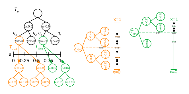
Figure 3: An example of intersection tree based on the partition. We show two BART models represented by $m=1$ tree.

Let $\mathcal{T}_{u}$ be a tree splitting on the latent variable $u$ inducing a partitioning of $[0,1]$. Then we use $\mathcal{T}_{x\mid\eta_{u}}$ to represent the tree splitting on the input variable $\bm{X}$ on the shard partition corresponding to the node $\eta_{u}$. The graphical representation is in Figure 3. Our sharded tree model is thus defined using $\mathcal{T}$ as

$$y(\bm{x}\mid\bm{u})=g(\bm{x},\bm{u};\mathcal{T},\bm{\beta})+\epsilon$$ (26)

and the posterior is,

$$\pi(\mathcal{T},\bm{\beta},\sigma^{2}|\bm{y},\bm{X},U)\propto L(\bm{y};\bm{X},\bm{U},\mathcal{T},\bm{\beta},\sigma^{2})\pi(\mathcal{T})\pi(\bm{\beta})\pi(\sigma^{2})$$

where $\pi(\bm{\beta}),\pi(\sigma^{2})$ follow their usual choices and $\pi(\mathcal{T})=\pi(h(\mathcal{T}_{x},\mathcal{T}_{u}))=\pi(\mathcal{T}_{x}\cap\mathcal{T}_{u})=\pi(\mathcal{T}_{x|\eta_{u}})\pi(\mathcal{T}_{u})=\pi(\mathcal{T}_{x})\pi(\mathcal{T}_{u})$, indicating that the sharding is independent of $\mathcal{T}_{x}$ a priori, and furthermore, taking $\pi(\mathcal{T}_{x|\eta_{u}})=\pi(\mathcal{T}_{x})$ informs independence of the prior on $\mathcal{T}_{x},$ i.e. the usual tree prior for $\mathcal{T}_{x}$ would be used. In particular, the typical depth prior for the regression tree component of the model is with respect to the root of the $\mathcal{T}_{x|\eta_{u}},$ not the root of the intersecting tree $\mathcal{T}.$

The posterior of interest is then recovered by marginalizing out $\bm{U}$, therefore, we are averaging over different possible shardings induced by $\mathcal{T}_{u}$:

$$\pi(\mathcal{T}_{x},\bm{\beta},\sigma^{2}|\bm{y},\bm{X})=\int_{\mathcal{T}_{u}}\int_{\bm{U}}\pi(\mathcal{T},\bm{\beta},\sigma^{2}|\bm{y},\bm{X},\bm{U})\pi(\mathcal{T}_{u})\pi(\bm{U})d\bm{U}d\mathcal{T}_{u}.$$

As foreshadowed, the choice of prior on $\mathcal{T}_{u}$ and the way how $\bm{U}$ is generated plays the key role in how the sharding affects the model. When $\mathcal{T}_{x\mid\eta}$ are all containing nothing more than a root node, then the intersected tree model admits a design that is completely determined by the sharding tree $\mathcal{T}_{u}$. In this situation, we want to optimize $B$-expected optimality criteria for the sharding tree (e.g.,(30)).

However, instead of carrying out a “frequentist direct optimization” to yield an optimal design for the tree, we take a Bayesian approach to sample from all possible designs for $\mathcal{T}_{u}$. When the $\mathcal{T}_{x\mid\eta}$ is no longer a root tree but with their own BART sum-of-tree structures, the problem of maximizing an optimality criteria of the whole intersected tree $\mathcal{T}_{u}\cap\mathcal{T}_{x\mid\eta}$ becomes intractable due to the size of search space. The Bayesian intuition in intersection tree is that if we conditioned on the structure $\mathcal{T}_{x\mid\eta}$’s, the optimal design of $\mathcal{T}_{u}$ will allow the posterior sampling from each $\mathcal{T}_{x\mid\eta}$ to converge much faster to the posterior mode. Nonetheless, a lot of insights could be achieved by considering the sharding induced by optimal design of $\mathcal{T}_{u}$, which coincides with the suggestion in Huggins et al. (2016).

3 Sharded Bayesian Additive Tree

In this section, we extend our construction of intersection tree model to what we call sharded Bayesian additive regression trees (SBT). The SBT model can be summarized as: Induce sharding using a single tree $\mathcal{T}_{u}$, and fit each shard using a BART $\mathcal{T}_{x\mid\eta}$ and aggregate.

3.1 Fitting and Prediction Algorithms

From the generic form of (2) and the specification in (26), we can write down our ensemble model,

$$y(\bm{x},\bm{u})=\sum_{k=1}^{B}\sum_{j=1}^{m}g(\bm{x};\bm{u}\mid\mathcal{T}_{x,j},M_{\mathcal{T}_{x,j}},\mathcal{X}_{k},\mathcal{T}_{u})+\epsilon,$$ (27)

Assuming $m=1$ for simplicity and marginalizing out the variable $u$, yield the formal expression:

$$y(\bm{x})=\sum_{b=1}^{B}w_{b}\cdot f_{b}(\bm{x};\mathcal{T}_{x\mid\eta_{b}},\bm{\beta})+\epsilon,$$ (28)

where we consider a set of weights $w_{1},\cdots,w_{B}$ from marginalization, whose sum $\sum_{b=1}^{B}w_{b}=1$ for a fixed number of shards $B$. We use $f_{b}(\bm{x};\mathcal{T}_{x\mid\eta_{b}},\bm{\beta})=\mathcal{T}_{x\mid\eta}$ (i.e., BART models for each $\eta_{u}$ leaf node) to emphasize that the additive components are from the collection $\mathcal{E}$, as defined by conditionally independent (but combined additively) BART models. The weights can be understood as “relative contribution” of each shard sub-model, and it is natural to ask the question of how to choose each of these $w_{b}$’s to attain an “optimal overall model”.

With our intersection tree topology in Figures 1, conditioning on each sharding induces a set of weights in our ensemble. When the distribution of auxilliary variable $\bm{U}$ and the tree structure of $\mathcal{T}_{u}$ are well-chosen, we can show that the resulting sharding tree model achieves the B-expected optimal design we defined above. In other words, the changing $\mathcal{T}_{u}$ (as $\mathcal{T}_{u}$ updates during MCMC iterations) serves as a collection of latent designs for weighting the BART models $f_{b}$ in the ensemble under consideration. To clarify the idea, we will introduce our fitting and prediction algorithms first, then provide different explanations of this procedure.

 

• Input. The full data set consisting of both $\bm{X},\bm{y}$. Tree priors for $\mathcal{T}_{u}$ and $\mathcal{T}_{x\mid\eta}$’s. The number of MCMC iterations $N_{MCMC}$ (See Appendix G for APIs).

• Output. Samples from the posteriors of $\mathcal{T}_{u}$ and $\mathcal{T}_{x\mid\eta}$’s.

1. Generate auxiliary variables $\bm{U}$. Sample $\bm{U}\sim\text{Unif(0,1)}$ i.i.d. and make the auxilliary dataset $\bm{V}=[\bm{X},\bm{U}]$.

2. For $k$ in $1:N_{MCMC}$ do

   1. Let $\mathcal{T}_{u}^{\text{old}}=\mathcal{T}_{u}$.

   2. Propose a regression tree $\mathcal{T}_{u}^{new}$ using some proposal.

   3. Partition $[0,1]$ using the partition representation of $\mathcal{T}_{u}$ by terminal nodes $\eta_{u}^{1},\cdots,\eta_{u}^{B}$ of $\mathcal{T}_{u}$, therefore, partition the data into $\bm{X}=\cup_{j=1}^{B}\bm{X}_{j}$.

   4. Compute the acceptance ratio $\tau=\max(1,\tau^{*})$.We use Metropolis-Hasting step $\text{Unif}(0,1)<\tau$ to decide whether accept:

   5. If accept, let $\mathcal{T}_{u}=\mathcal{T}_{u}^{\text{new}}$. If reject, let $\mathcal{T}_{u}=\mathcal{T}_{u}^{\text{old}}$.

   6. For each terminal node $\eta_{u}^{j}$ of $\mathcal{T}_{u}$ do

      1. Let $\mathcal{T^{\text{old}}}_{x\mid\eta_{u}^{j}}=\mathcal{T}_{x\mid\eta_{u}^{j}}$.

      2. Propose a regression tree $\mathcal{T}_{x\mid\eta_{u}^{j}}$ with $\bm{X}_{j}$ as input; $\bm{y}_{j}$ as output (with the tree priors for $\mathcal{T}_{x\mid\eta_{u}^{j}}$) including splitting point. Denote this $\mathcal{T}_{x\mid\eta_{u}^{j}}$ as $\mathcal{T}_{x\mid\eta_{u}^{j}}^{\text{new}}$.

      3. Compute the acceptance ratio

         $$\tau_{j}=\max\left(1,\frac{\ell\left(\left.\mathcal{T}_{x\mid\eta_{u}^{j}}^{\text{new}}\right|\bm{X}_{j},\bm{y}_{j},\bm{u},\mathcal{T}_{u}\right)}{\ell\left(\left.\mathcal{T}_{x\mid\eta_{u}^{j}}^{\text{old}}\right|\bm{X}_{j},\bm{y}_{j},\bm{u},\mathcal{T}_{u}\right)}\right),$$

         and use Metropolis-Hasting step $Unif(0,1)<\tau_{j}$ to decide whether accept.

      4. If accept, let $\mathcal{T}_{x\mid\eta_{u}^{j}}=\mathcal{T}_{x\mid\eta_{u}^{j}}^{\text{new}}$ and update the likelihoods. If reject, let $\mathcal{T}_{x\mid\eta_{u}^{j}}=\mathcal{T}_{x\mid\eta_{u}^{j}}^{\text{old}}$.

   7. Update the BART sub-model parameters as usual, and append the $\mathcal{T}_{u}$ and $\mathcal{T}_{x\mid\eta_{u}^{j}}$’s to the output array.

 

Algorithm 1 Sharded Bayesian regression trees fitting algorithm.

Algorithm 1 allows us to draw samples from the posterior of the $\mathcal{T}_{u}$ and $\mathcal{T}_{x\mid\eta_{u}^{j}}$, conditioned on the data only. In Algorithm 1 step 2d, the proposal distribution factors $p\left(\left.\mathcal{T}_{u}^{\text{new}}\right|\bm{u}\right)$ and $p\left(\left.\mathcal{T}_{u}^{\text{old}}\right|\bm{u}\right)$ represent how likely the sharding tree structure $\mathcal{T}_{u}$ can be proposed given the auxilliary variable $u$. The sharding tree structure $\mathcal{T}_{u}$ partitions the input $\bm{X}$ into shards $\bm{X}_{j},j=1,\cdots B$; and simultaneously partitions responses $\bm{y}$ into shards $\bm{y}_{j},j=1,\cdots,B$. This step immediately reveals the fact that we cannot perform fitting of $\mathcal{T}_{u}$ and $\mathcal{T}_{x\mid\eta_{u}^{j}}$ separately, since a newly proposed $\mathcal{T}_{u}$ immediately determines the $\ell\left(\left.\mathcal{T}_{x\mid\eta_{u}^{j}}\right|\bm{X}_{j},\bm{y}_{j}\right)$ in the same expression.

Note that we do not update the whole intersection tree structure $\mathcal{T}_{u}\cap\mathcal{T}_{x}$ jointly, but update $\mathcal{T}_{u}$ and $\mathcal{T}_{x\mid\eta_{u}}$’s sequentially. Theoretically, we can equivalently perform a joint update using the following accept-reject ratio $\max(1,\tau^{*})$ where

$$\tau^{*}=\frac{\left[\prod_{j=1}^{B}\ell\left(\left.\mathcal{T}_{x\mid\eta^{j}_{u}}\right|\bm{X}_{j}^{\text{new}},\bm{y}_{j}^{\text{new}}\right)\right]\cdot p\left(\left.\mathcal{T}_{u}^{\text{new}}\right|\bm{u}\right)}{\left[\prod_{j=1}^{B}\ell\left(\left.\mathcal{T}_{x\mid\eta^{j}_{u}}\right|\bm{X}_{j}^{\text{old}},\bm{y}_{j}^{\text{old}}\right)\right]\cdot p\left(\left.\mathcal{T}_{u}^{\text{old}}\right|\bm{u}\right)}.$$

This requires us to propose not only $\mathcal{T}_{u}^{\text{new}}$ but also all $\mathcal{T}_{x\mid\eta_{u}^{j}}^{\text{new}},j=1,\cdots,B$ jointly at the same time since we want to obtain a new intersection tree structure. This formulation would eliminate the need of additional inner loop in step 2f and the computation of accept-reject ratio in step 2(f)iii, compared to the current Algorithm 1. However, this joint proposal would practically result in slow computation and mixing in MCMC due to its high dimensional nature. Also, such a joint proposal is not suitable for parallel computation. Instead, we utilize the Metropolis-Hasting step as shown below.

In Algorithm 1 step 2(f)ii, we note that such a tree $\mathcal{T}_{u}$ is still partitioning the whole domain $\mathcal{X}$, although its structure is completely dependent on $\bm{X}_{j}$. After fitting the SBT model, we want to use the posterior sample sequence of $\mathcal{T}_{u}$ and $\mathcal{T}_{x\mid\eta_{u}}$’s. The prediction algorithm is slightly different since, as shown below, the auxiliary variable $u_{*}$ needs to be drawn as well. This Algorithm (2) gives one sample of $g(x_{*}\mid\mathcal{T}_{x\mid\eta_{x_{*}}},\mathcal{T}_{u},u_{*})$.

 

• Input. Samples from the posteriors of $\mathcal{T}_{u}$ and $\mathcal{T}_{x\mid\eta}$’s. Predictive location $x_{*}$. The number of MCMC iterations $N_{MCMC}$.

• Output. Predictive value from SBT at location $x_{*}$.

1. For $k$ in $1:N_{MCMC}$ do

   1. Sample $u_{*}\sim\text{Unif(0,1)}$ and make the auxilliary point $(x_{*},u_{*})$.

   2. Input $u_{*}$ to the regression tree $\mathcal{T}_{u}$ with $u_{*}$ as input; Denote the terminal node where $u_{*}$ falls as $\eta_{u_{*}}$

   3. Input $x_{*}$ to the regression tree $\mathcal{T}_{x\mid\eta_{u_{*}}}$ with $x_{*}$ as input; $\hat{y}(x_{*})=\mathcal{T}_{x\mid\eta_{u_{*}}}(x_{*})$ as output.

   4. Append $\hat{y}(x_{*})$ as predicted value to the prediction sample sequence.

2. Take the average of prediction sample sequence as predictive value at location $x_{*}$.

 

Algorithm 2 Sharded Bayesian regression trees predicting algorithm.

3.2 Perspectives on BART Ensembles

Since we are building SBT as a Bayesian model, more insightful perspectives are needed. The following two perspectives are two sides of one coin, depending on whether we want to study the empirical measure derived from individual sharded trees (“as it is”) or we want to infer the marginalized measure for the tree population first, and then take inference. Both perspectives happen on the space of tree structures, precisely for the tree structure $\mathcal{T}_{u}$, admitting the same algorithms above.

Perspective one is to treat the ensemble model as a weighted aggregation. In this perspective, the weights determined by the tree $\mathcal{T}_{u}$ does not marginalize this tree structure out but treat this fixed structure as if it is the MAP of the tree posterior. This perspective suggests that the sharded models are individual but not independent, and an aggregated model produced by (re-)weighting of these representatives would do us a better job.

Perspective two is to treat the ensemble model as averaging over the probability distribution defined by the (normalized) weights. In this perspective, the weights determined by the tree $\mathcal{T}_{u}$ are considered as an empirical approximation to a marginalized model, where $\mathcal{T}_{x\mid\eta_{u}}$’s are fitted as new tree models and we want to marginalize the effect of sharding introduced by $\mathcal{T}_{u}$. If we use regression tree as an “interpretable” decision rule in the sense of Rudin et al. (2022), then this perspective ask us to derive the decision rule by coming up with just one margnalized rule: for a new hypothetical $x^{*}$, run through the marginalized measure and compute the mean model, then we have $1$ result as our final rule.

3.3 Weights of sub-models

Although we have provided two different perspectives on the ensemble model, we have not yet described the effect of our weights. There are two lines of literature we briefly recall below.

First, from the generalized additive model literature (McCullagh and Nelder, 2019; Strutz, 2011), the choice of weights are motivated by reducing the uncertainty in prediction or the heteroscedasticity in observations based on the design (Cressie, 1985). For example, in the weighted least square regression, the weights are chosen to be inverse proportional to the location variances, meeting D-optimality in the regression setting.

Second, from the model aggregation literature, research has focused on how to improve the accuracy of prediction (Barutcuoglu and Alpaydin, 2003) and introduce adaptive and dynamic weighting to improve the overall accuracy of the ensemble (Kolter and Maloof, 2007). And more recent works formulate the choice of weights in regression ensembles as an optimization meta-problem to be solved (Shahhosseini et al., 2022).

Under the assumption of a $B$-expected optimal design, we can achieve a uniform posterior rate for the aggregated model when the underlying function has homogeneous smoothness. This echoes the claim by Ročková and Saha (2019) that the Galton-Watson prior would ensure a nearly optimal rate not only for single BART but also in an aggregated scheme. We restate their main result using our notations below and provide a brief intuitive explanation afterwards.

Theorem 8.

(Theorem 7.1 in Ročková and Saha (2019) on the posterior concentration for BART) Assume that the ground-truth $f_{0}$ is $\nu$-Holder continuous with $\nu\in(0,1]$ where $\|f_{0}\|_{\infty}\apprle\log^{1/2}n$. Denote the true function as $f_{0}$ and the BART model based on an ensemble $\mathcal{E}$ as $f_{b}$, and the empirical norm $\|f\|_{n}\coloneqq\frac{1}{n}\sum_{i=1}^{n}f(\bm{x}_{i})^{2}$.

Assume a regular design $\bm{X}=\{\bm{x}_{1},\cdots,\bm{x}_{n}\}\subset\mathbb{R}^{d}$ (in the sense of Definition 3.3 of Ročková and van der Pas (2019)) where $d\lesssim\log^{1/2}n$. Assume the BART prior with the number of trees $T$ fixed, and with node $\eta$ splitting probability $p_{split}(\eta)=\alpha^{\text{depth}(\eta)}$ for $\alpha\in[1/n,1/2)$. With $\varepsilon_{n}=n^{-\alpha/(2\alpha+d)}\log^{1/2}n$ we have

$$\prod\left(\left.f_{b}\in\mathcal{F}:\left\|f_{0}-f_{b}\right\|_{n}>M_{n}\varepsilon_{n}\right|\bm{y}_{n}\right) \rightarrow 0,$$

for any sequence $M_{n}\rightarrow 0$ in $P_{f_{0}}$-probability, as the sample size $n$ and dimensionality $d\rightarrow\infty$.

The functional space $\mathcal{F}$ of step-functions is defined the same as in Ročková and van der Pas (2019). The regularity assumption for the design points aims at ensuring that the underlying true signal $f_{0}$ can be approximated by the BART model. Based on this result, we can extend the posterior concentration to the sharded-aggregation model. And then from this result below, we know the choice of weights would affect this rate.

Theorem 9.

Under the same assumptions and notations as in Theorem 8, we suppose that the sharding tree $\mathcal{T}_{u}$ partitions the full dataset $\bm{X}=\{\bm{x}_{1},\cdots,\bm{x}_{n}\}\subset\mathbb{R}^{d}$, $\bm{y}_{n}$ into $B$ shards $\mathcal{X}_{b},b=1,\cdots,B$ and corresponding responses $\bm{y}_{b,n_{b}},\cup_{b=1}^{B}\bm{y}_{b,n_{b}}=\bm{y}_{n}$. We designate a set of weights $w_{1},\cdots,w_{b}$ whose sum $\sum_{b=1}^{B}w_{b}=1$ for fixed number of shards $B$. Then, our sharded-aggregation model would take the form of $\sum_{b=1}^{B}w_{b}f_{b}$ where $f_{b}$ is the BART based on the shard $\bm{y}_{b,n_{b}}$.

$$\prod\left(\left.\left\|f_{0}-\sum_{b=1}^{B}w_{b}f_{b}\right\|_{n}>M_{n}B\cdot\varepsilon_{n}\right|\bm{y}_{n}\right)$$ (29)

$$\leq B\cdot\max_{b=1,\cdots,B}\prod\left(\left.f_{b}\in\mathcal{F}:\left\|f_{0}-f_{b}\right\|_{n_{b}}>w_{b}^{-1}\cdot M_{n}\varepsilon_{b,n}\right|\bm{y}_{b,n_{b}}\right)\leq B\varepsilon_{n}.$$

Then, the aggregation of sharded tree posteriors also concentrate to the the ground-truth $f_{0}$.

Proof.

See Appendix E. ∎

For single tree regression, we motivate the optimal choice of sharding sizes to be inversely proportional to the probability mass contained in the sharded region (see Proposition 4), which aligns with the spirit of the aforementioned literature. As a Bayesian model, the posterior contraction rate is more or less a key element in ensuring the accuracy of posterior prediction.

The following corollary follows from the exchangeability of data shards among different sub tree model, when each sub-model is based on sharding induced by $\mathcal{T}_{u}$. The rationale for the corollary is that the RHS of (29) is a maximum bound that depends on $\varepsilon_{n}\coloneqq\min_{b=1,\cdots,B}\varepsilon_{b,n}$ and $\varepsilon_{b,n}\coloneqq n_{b}^{-\alpha/(2\alpha+d)}\log^{1/2}n_{b}$ subject to $\sum_{b=1}^{B}n_{b}=n$.

Regardless of the choice of $M_{n}$, the $\varepsilon_{n}$ is minimized when all $w_{b}^{-1}\cdot\varepsilon_{b,n}$ are “as close to each other” as possible, following a similar argument like Lemma 2, and we know that $w_{b}^{-1}\cdot\varepsilon_{b,n}$ need to be all equal as well in order to minimize RHS.

Corollary 10.

Under the same assumptions as in Theorem 9, the RHS of (29) is minimized if the products of weights and shard sizes, $w_{b}^{-1}\cdot n_{b}^{-\alpha/(2\alpha+d)}\log^{1/2}n_{b}$, are all equal.

Immediately, this asks us to put weights that are roughly proportional to $\varepsilon_{b,n}$, and when the $\mathcal{T}_{u}$ satisfies $B$-expected optimal design when $U$ is uniform, $n_{b}$ are “roughly equal”, and therefore the optimal design would require us to put roughly equal weights onto each shard BART. In other words, $\mathcal{T}_{u}$ having a $B$-expected optimal design is a sufficient and necessary condition for equally-weighted aggregation to have optimal posterior concentration rate when the underlying function is homogeneously smooth.

This also indicates that if it happens that we need to create shards of different sizes (e.g., we have different amount of computational resources for different shards), we can adjust the weights for each shards $w_{b}(n)$ (as a function of sample size $n$) to account for different growth rates.

4 Experiments and Applications

We first focus on examining the empirical performance based on simulations, where our dataset is drawn from synthetic functions without any amount of noise. We focus on varying the parameter $\mathtt{shardepth}$ which defines the depth of $\mathcal{T}_{u}$, and therefore the (maximum) number of shards (see Appendix G).

For clarity in figures, we use letters A to F associated with the boxplots for BART and SBT comparisons in the current section. For A, B and C, we fit and predict using BART with 25%, 50% and all of the training set as baseline models. For D, E and F, we fit our SBT model using full training set but different combinations of model parameters $\mathtt{shardepth}=0,1,2$. Precisely, we use: A: BART with 25% training set, B: BART with 50% training set, C: BART with full training set, D: SBT with $\mathtt{shardepth}=0$, E: SBT with $\mathtt{shardepth}=1$, F: SBT with $\mathtt{shardepth}=2$. We summarize the trade-off between model complexity and goodness-of-fit using out-of-sample RMSE and coverage, and also show that the SBT model is less computationally expensive compared to the standard BART model.

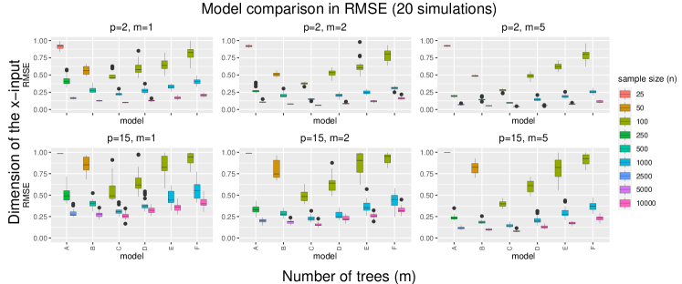
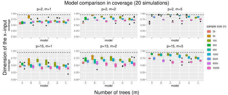
Figure 4: Comparison (in RMSE and 95% (indicated by dashed line) confidence interval coverage) between standard BART (with 100%, 50% and 25% of all samples) and our sharded BART model with different $\mathtt{shardepth}$(=0,1,2). We design two experiments using branin function defined on $p=2,15$ dimensional domains (displayed in panel rows); with each kind of tree model with $m=1,2,5,10,20$ trees (displayed in panel columns). In each panel, we study the sample of sizes $n=100,1000,10000$.

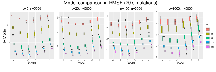
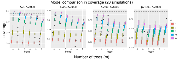
Figure 5: Comparison (in RMSE and 95% (indicated by dashed line) confidence interval coverage) between standard BART (with 100%, 50% and 25% of all samples) and our sharded BART model with different $\mathtt{shardepth}$(=0,1,2). We design four experiments using $n=5000$ samples from friedman function defined on $p=5,20,100,1000$ dimensional domains (displayed in panel columns). In each panel, we study the number of trees $m=1,2,5,10,20$ in each model.

4.1 Small-sample on synthetic functions

In Figure 4, we present model comparison based on 20 different fits on the same dataset with different sample sizes $n$ and dimensionality $p$, drawn from the Branin function defined on $p=2$ and $p=15$ dimensional domains. For the low dimensional situation ($p=2$), we compare the SBT with $\mathtt{shardepth}=1$ with BART using $0.25n$ samples, and analogously for $\mathtt{shardepth}\in\{0,2\}$. This shows that the RMSE of SBT and standard BART (with the same expected sample size) are comparable regardless of the number of trees $m$. Meanwhile, the 95% confidence interval coverages decreases with increasing sample size $n$, and increasing number of trees $m$. However, when $n=10000$, the SBT model has improved coverage compared to a standard BART of the corresponding sample sizes. For the high dimensional situation ($p=15$), the trends observed in the low dimensional situation remains to be true, but the RMSE is inflated and the coverage is deflated, as expected.

In Figure 5, we present model comparison based on 20 different fits on the same dataset with the same sample size $n=5000$ but different dimensionality , drawn from the Friedman function defined on $p=5,20,100,1000$ dimensional domains. Here we fix the sample size, and observe that SBT generally gives a worse RMSE compared to the standard BART model, but the difference in RMSE decreases as dimensionality increases. Increasing the number of trees in each BART or SBT model will improve the RMSE performance but the effect of $\mathtt{shardepth}$ is less obvious as $p$ changes. In terms of 95% credible interval coverages, the SBT is closer to standard BART with full sample size $n$, avoiding the inflated coverage caused by using a smaller sample size $0.5n$ or $0.25n$.

This experiment shows that with small samples, our algorithm could also work well: (i) ideally $\mathcal{T}_{u}$ shows no sharding behavior; and (ii) even with some coarse sharding, the aggregated posterior is not bad for small samples.

4.2 Real-world data: redshift simulation

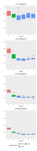
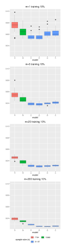
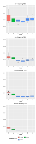
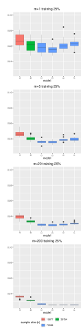
Figure 6: Model comparison in terms of RMSE on testing sets (as complement set of training set from the original redshift dataset). From the left to the right columns, the training set is taken as 5%, 10%, 15%, 20%, 25% randomly selected samples from the original dataset; from the top to the bottom rows, the number of trees varies from $m=1,5,20,200$. In each of the panels, we use boxplots to display the performance metric distribution from 20 simulations; and color to denote the actual training set sample sizes corresponding to each model.

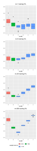
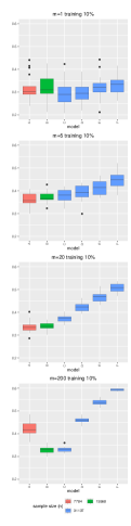
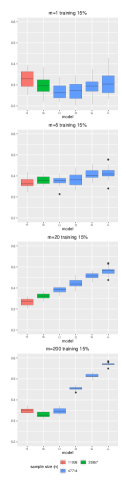
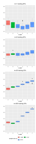
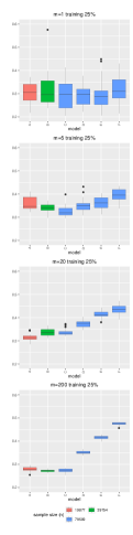
Figure 7: Model comparison in terms of coverage of 95% confidence intervals. From the left to the right columns, the training set is taken as 5%, 10%, 15%, 20%, 25% randomly selected samples from the original redshift dataset; from the top to the bottom rows, the number of trees varies from $m=1,5,20,200$. In each of panels, we use boxplots to display the performance metric distribution from 20 simulations; and color to denote the actual training set sample sizes corresponding to each model.

In this real-world application, we studied a redshift simulator dataset from cosmology (Ramachandra et al., 2022). The dataset contains 6,001 functional observations from a redshift spectrum simulator. For a combination of 7 different cosmological parameters (e.g., metallicity, dust young, dust old and ionization etc.), we can observe and collect the spectrum function as vectors of different lengths (ranging from 48 to 100 points), under the configuration defined by these set of cosmological parameters. This presents essential challenges to the modeling task due to its multi-output nature and observation size. Typically, one emulates the multivariate vector output depending on the cosmological parameters using statistical models, in our case BART and SBT.

We provide the RMSE for different models in Figure 6, where we can see that BART and SBT model with full training sets always has the overall smaller RMSE. Regardless of the training set size and model parameters, as soon as the number of trees $m$ is greater than 2, the SBT has similar RMSE and the difference between BART and SBT is negligible when $m\geq 20$, and SBT is slightly better for larger $m$’s. This ensures that SBT has competitive estimation and prediction performance compared to BART. And the RMSE also slightly decreases as the $m$ increases in SBT and BART.

The more interesting observations come from Figure 7. When $m\geq 2$, the SBT can have the best performance when the $\mathtt{shardepth}\geq 1$, indicating that a deeper sharding tree $\mathcal{T}_{u}$ leads to better coverage in confidence intervals. When $m\geq 5$, SBT always shows better coverage than BART regardless of the choice of other SBT model parameters, but a deeper sharding tree $\mathcal{T}_{u}$ still presents the best coverage. With all the rest model parameters fixed, the coverage also increases significantly as $m$ increases in SBT; but not so obviously in BART.

From this analysis, we confirm that SBT can fit as well as BART but provides much better fitting efficiency and coverage with deeper $\mathcal{T}_{u}$ on real-world large datasets.

4.3 Complexity Trade-offs

The model complexity (Kapelner and Bleich, 2016; Bleich and Kapelner, 2014) and computational complexity (Pratola et al., 2014) are two important topics in BART and its variants. In the original BART algorithm, the complexity can be derived as follows. Our result is parallel to the computational complexity for spanning trees as shown in Luo et al. (2021).

From the previous experiments, we show how the depth of the tree $\mathcal{T}_{u}$ in SBT trades off with goodness-of-fit of each $\mathcal{T}_{x\mid\eta}$. Fixing the structures of (each of) the trees $\mathcal{T}_{x\mid\eta}$, when we have finer partitions induced by $\mathcal{T}_{u}$, the shard model fit would become worse because each shard tends to have less data. However, shards become smaller and hence speeds up the model fitting, until it hits the communication cost bottleneck.

Lemma 11.

(Computational complexity for BART) Assuming that there are at most $k_{i}$ nodes for the $i$-th tree for $i=1,\cdots,m$ trees, the worst-case computational complexity for each MCMC step in BART is $\mathcal{O}(m^{2}\cdot n^{2}+\sum_{i=1}^{m}k_{i})$.

Proof.

See Appendix F. ∎

This worst-case complexity does grow with the sample size $n$, but theoretically there is not an explicit relation between $\max_{i}n_{i}$, $B$ and $n$ in BART. Based on this lemma, we have the following result directly from the model SBT construction.

Lemma 12.

Suppose that there are $k$ nodes for a complete binary tree $\mathcal{T}$, and there are $n$ samples fitted to the tree structure. The number of all nodes $k$ and the sample size $n$ satisfies $1\leq k\leq 2n$.

Proof.

The terminal nodes must be non-empty and contain at least one sample. In a complete binary tree, there can be at most $\log n$ layers, hence the total number of internal nodes is bounded by $n\cdot\sum_{\eta=0}^{\log n}2^{-\eta}=n\cdot(2-2^{-\log n})\leq 2n$. ∎

Corollary 13.

(Computational complexity for BART, continued) Assuming that there are at most $n_{i}=n$ samples for the $i$-th tree for $i=1,\cdots,m$ trees, the worst-case computational complexity for each MCMC step in BART is $\mathcal{O}(m^{2}n^{2})$.

These two lemmas immediately gives the following complexity result for SBT model.

Proposition 14.

(Complexity for SBT) Let the $\mathcal{T}_{u}$ in SBT be of depth $k$ (at most $2^{k}$ leaf nodes), and assume that there are at most $n_{j}$ samples for each of the $m_{j}$ single trees in the $j$-th BART, the worst-case computational complexity for each MCMC step in SBT is $\mathcal{O}\left(n^{2}+\sum_{j=1}^{2^{k}}m_{j}^{2}n^{2}_{j}\right)$. Specifically, when we choose $\bm{U}$ uniformly thus creating equal sized shards (in expectation) of size $n_{j}=n/2^{k}$ and take the same number $m$ of trees in each BART, the above complexity for SBT becomes $\mathcal{O}\left(n^{2}+m^{2}\cdot n^{2}/2^{k}\right)\rightarrow\mathcal{O}(n^{2})$ as $k\rightarrow\infty$.

If we take equal sized shards and the same number of trees, it follows directly from the proposition that the depth $k$ of $\mathcal{T}_{u}$ controls the complexity of SBT, and when $k=0$ it reduces to BART complexity as expected. We can see that SBT is strictly better than BART in terms of complexity, but shallower $\mathcal{T}_{u}$ has less complexity advantage. However, the big advantage of SBT is that updates at and below each leaf node of $\mathcal{T}_{u}$ can be done in parallel and that implementation reduces the complexity of SBT to $\mathcal{O}\left(n^{2}+\max_{j}m_{j}^{2}n^{2}_{j}\right)$.

5 Discussion

In this paper, we introduce the (randomized) sharded Bayesian tree (SBT) model, which is motivated from inducing data shards from the optimal design tree $\mathcal{T}_{u}$ and assemble sub-models $\mathcal{T}_{x\mid\eta_{u}}$’s within the same model fitting procedure. This idea describes a principled way of designing a distribute-aggregate regime using tree-partition duality. The closest relative in the literature is Chowdhury and Jermaine (2018) and Scott et al. (2016). Compared to Chowdhury and Jermaine (2018), we did not parallelize at the MCMC level but instead at the model level and therefore we do not have to enforce additional convergence conditions. Compared to Scott et al. (2016), we propose a new model that links the optimal sharding and convergence rate in an explicit manner.

The SBT construction puts the marginalization into the model construction, showing the additive structure can be leveraged to realize data parallelism and model parallelism. Our modeling method shares a spirit from both lines of research. On one hand, we define the partition by an random measure $\mathbb{P}$, where Chowdhury and Jermaine (2018) introduce auxilliary variables to ensure MCMC convergence. In SBT, we perform model averaging between shard models which is justified by optimal designs from $\mathcal{T}_{u}$ and optimal posterior contraction rates of BART, which is a novel perspective when applied in conjunction with randomization. However, our averaging is done “internal to the model” and maintains an interpretable partition rule (given by internal nodes of $\mathcal{T}_{u}$) within this framework.

Motivated by scaling up the popular BART model to much larger datasets, we identify and address the following challenges for applying the distribute-aggregate scheme for the regression tree model from theoretical perspectives.

1. It is unclear how to design data shards $\mathcal{X}_{i}$’s when the parameter space is not finite dimensional (e.g., trees), and the previous work focus on improving the convergence behavior (Chowdhury and Jermaine, 2018). We answer this question from an optimal design (of $\mathcal{T}_{u}$) perspective, that is, probability inverse allocation is optimal.

2. It is unclear how to choose the weights $w_{i}$ and the number of shards $B$ that is appropriate to the dataset from a theoretically justifiable perspective (e.g., reciprocal of variances) (Scott et al., 2016). We answer this question by calibrating posterior contraction rates, stating that for BART, the weights (in SBT) that lead to fastest posterior convergence are determined by the sample size and the smoothness of the actual function.

3. It is unclear how to generalize the distribute-aggregate paradigm to summarize and possibly reduce the sum-of-tree or general additive (Bayesian) model (Chipman et al., 2010). We design a novel additive tree model to incorporate this regime within the framework of the BART construction and show better complexity can be attained using SBT.

The SBT model introduces randomizations into the model fitting and prediction procedure, and attain strictly lower complexity compared to the original BART model. Our aggregation regime is justified by optimal design for $\mathcal{T}_{u}$ under uniform distribution and optimal posterior contraction rates. As supported by the experiments on simulation and real-world big datasets, we have not only witnessed its high scalability but also the improvement in terms of RMSE under appropriate parameter configurations. The complexity advantage can be practically improved in the parallel setting.

Appendix A Distribution of $\bm{U}$

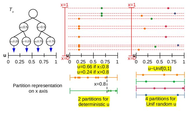
Figure 8: A balanced tree of depth $k=2$ and its pruned subtree which induced partition on $[0,1]$. This figure shows how completely deterministic rule for $\bm{U}$ (middle column) and how uniform random rule for $u$ (right column) create different sharding on the same dataset $\bm{X}$ (10 dots) on $[0,1]$.

This section shows an example on the effect of choosing different distributions for the augment random variable $u$. Suppose that $\mathcal{T}_{u}$ is a fully balanced binary tree consisting of $B$ terminal nodes. Here we examine two different rules conditioned on the balanced partition tree $\mathcal{T}_{u}$ at depth $k=2$ as illustrated in Figure 8. Conditioning on the tree structure $\mathcal{T}_{u}$, if we choose the uniform variable $\bm{U}\sim\text{Unif}(0,1)$ independent of $\bm{X}$, then we partition the dataset into shards with approximately equal sized 4 shards (where the approximation would become exact in the limit $n\rightarrow\infty$).
They are evenly distributed over $[0,1]$, overlap, and display completely random designs.

Conditioning on the same $\mathcal{T}_{u}$ structure, if we choose the variable $\bm{U}$ determined by $\bm{X}$ in some manner, say using the rule $U=\begin{cases}0.66&x\leq 0.8\\ 0.24&x>0.8\end{cases}$, (which can be described by another tree) then we partition the dataset into 2 shards of sizes 3 and 7 with no intersection. They are supported in $[0,1]$, do not overlap, and displays deterministic designs. If we choose the $\bm{U}$ randomly as we will show below, the sharded datasets allocated to each terminal leaf node can follow an optimal design within the corresponding partition with a good chance.

Appendix B Optimal Design for Constrained Leaves

Figure 9: We generate $n=1000$ random multinomial samples with equally probabilities $1/B$ being assigned to $B=4$ (top) and $B=8$ (bottom) leaf nodes, and then compute the $\phi_{n}(\bm{u}_{1},\ldots,\bm{u}_{n}\mid\mathcal{T})$ defined in (22) for 1000 different multinomial draws and assign them to these leaves. We display 2000 batches of assignments using histogram (left column) and boxplot (right column). We indicate the $\phi_{n}^{\max}$ using violet dashed lines in both plots. The probability of getting at $\phi_{n}^{\max}=\frac{n!}{q!^{(B-r)}(q+1)!^{r}}\frac{1}{B^{n}}$ using the notation in Lemma 2.

We have seen from Figure 9, that ss the number of leaves $B$ increases, the chance that a random assignment attains optimal design tends to zero.

More generally, we want to solve the optimization problem $\max_{(n_{1},\cdots,n_{B})}\prod_{b=1}^{B}n_{b}$, with constraints $\sum_{b=1}^{B}n_{b}=n$ and $n_{b}^{-}\leq n_{b}\leq n_{b}^{+}$, i.e., we need to keep minimum and maximum sample sizes for each leaf. This kind of scenario is not uncommon, for instance, the tree has already contain several pilot samples and we want to find the optimal design conditioned on these pilot samples. Note that this can be solved using integer programming as explained below, and we still assume that $B\leq n$.

Case I: Trivial constraints.

When $n_{b}^{-}\leq\frac{n}{B}\leq n_{b}^{+}$ for all $b$, this reduces to Lemma 2.

Case II: Nontrivial constraints.

Otherwise, there are some $b$ such that $\frac{n}{B}\notin[n_{b}^{-},n_{b}^{+}]$. Then, we consider the equivalent problem

$$\max_{(n_{1},\cdots,n_{B})}\sum_{b=1}^{B}\log n_{b}\text{ s.t. } \sum_{b=1}^{B}n_{b}=n,$$ (30)

$$n_{b}^{-}\leq n_{b}\leq n_{b}^{+},$$

where $n_{b}$ are integer indeterminates of the diagonal entries in the design matrix, and also the number of samples assigned to leaf $b$. This is closely related to the closest point search problem on lattice $\mathbb{N}^{B}$(Agrell et al., 2002), where a polynomial time algorithm is possible when the dimension $B$ is fixed.

However, the problem (30) comes with non-trivial constraints, and the lattice $\mathbb{N}^{B}$ is special since its reduced basis is the canonical basis. Therefore, we take a different approach below.

To begin with, for $B$ indeterminates $n_{1},\cdots,n_{B}$, geometrically we can perceive the problem as finding a point in

$$R\cap\mathbb{N}^{B}\cap C,R\coloneqq\left\{\left(n_{1},\cdots,n_{B}\right)\mid\sum_{b=1}^{B}n_{b}=n\right\}$$

$$C\coloneqq\left\{\left(n_{1},\cdots,n_{B}\right)\mid n_{b}^{-}\leq n_{b}\leq n_{b}^{+},b=1,\cdots,B\right\}$$

such that it has the closest $L_{2}$ distance (or any convex distance would work) to the point $\left(\frac{n}{B},\cdots,\frac{n}{B}\right)\in\mathbb{R}^{B}$, which is possibly not in the $R\cap\mathbb{N}^{B}$.

Then, we can consider the following problem of finding the closest point $\bm{n}=(\hat{n}_{1},\cdots,\hat{n}_{B})\in C$ on the hyperplane defined by $\bm{1}\cdot\bm{n}-n=0$, to the continuous solution to (30), i.e., $\left(\frac{n}{B},\cdots,\frac{n}{B}\right)$. The point on the hyper-plane distance that minimizes the followin $d(\bm{n})\equiv d(\hat{n}_{1},\cdots,\hat{n}_{B})\coloneqq\left(\frac{\left|\sum_{b=1}^{B}\hat{n}_{b}-n\right|}{\sqrt{B}}\right)^{2}+\sum_{b=1}^{B}\left(\hat{n}_{b}-\frac{n}{B}\right)^{2}$, and we convert the problem into following format, which is usually easier to solve numerically with fewer constraints (and remove the strict constraint $\sum_{b=1}^{B}n_{b}=n$).

$$\min_{\bm{n}}d(\bm{n}),\text{ s.t., }\bm{n}\in C.$$ (31)

Proposition 15.

A solution to (31) in $\bm{n}$, is a solution to (30).

Proof.

Without loss of generality, we can assume that the integer vector $\left(\hat{n}_{1},\hat{n}_{2},\hat{n}_{3},\cdots,\hat{n}_{B}\right)$ is a solution to (31), but is not a solution to (30). We proceed by contradiction. Suppose that we only need to perform a $\pm 1$ operation and change it into $\left(\hat{n}_{1}+1,\hat{n}_{2}-1,\hat{n}_{3},\cdots,\hat{n}_{B}\right)$, to yield a larger value of (30). We can focus on the first two coordinates and a difference of mass 1, since all entries are non-negative integers and their sum is fixed to be $n$, we can perform induction on the number of different entries and the number of $\pm 1$ operations based on this base case. That means, $\log(\hat{n}_{1})+\log(\hat{n}_{2})<\log(\hat{n}_{1}+1)+\log(\hat{n}_{2}-1)$, and $\log\left(\frac{\hat{n}_{1}}{\hat{n}_{1}+1}\right)=\log\left(1-\frac{1}{\hat{n}_{1}+1}\right)<\log\left(\frac{\hat{n}_{2}-1}{\hat{n}_{2}}\right)=\log\left(1-\frac{1}{\hat{n}_{2}}\right)$. This implies $\hat{n}_{2}-\hat{n}_{1}>1\Longrightarrow\hat{n}_{1}-\hat{n}_{2}+1<0$ for integers $\hat{n}_{1},\hat{n}_{2}$, hence the first term in $d(\hat{n}_{1},\hat{n}_{1}+1,\hat{n}_{3},\cdots,\hat{n}_{B})$ remains the same; yet the second term differ by

$$\left[\left(\hat{n}_{1}+1-\frac{n}{B}\right)^{2}+\left(\hat{n}_{2}-1-\frac{n}{B}\right)^{2}\right]-\left[\left(\hat{n}_{1}-\frac{n}{B}\right)^{2}+\left(\hat{n}_{2}-\frac{n}{B}\right)^{2}\right]$$

$$= 2\left(\hat{n}_{1}-\frac{n}{B}\right)+1-2\left(\hat{n}_{2}-\frac{n}{B}\right)+1$$

$$= 2\left(\hat{n}_{1}-\hat{n}_{2}+1\right)<0,$$

contradicting the assumption that $\left(\hat{n}_{1},\hat{n}_{2},\hat{n}_{3},\cdots,\hat{n}_{B}\right)$ is a solution to (31). ∎

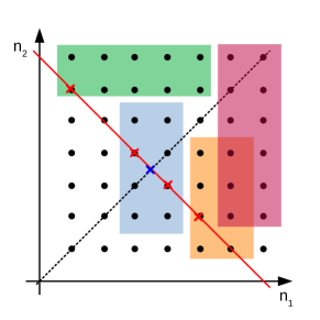
Figure 10: Geometric intuition of proof for constrained optimal design. We display a $\mathbb{N}^{2}$ lattice on the $\mathbb{R}^{2}$ plane, the fixed sum $n_{1}+n_{2}=n(=7)$ is displayed as red solid line, crossing all 7 possible pairs $(1,6),(2,5),\cdots,(6,1)$. The continuous solution to (30) is displayed by the blue cross, i.e., the pair $(3.5,3.5)$.
If the constrained region (e.g., the blue region covers the $(3.5,3.5)$, while the green and orange regions do not) and has non empty intersection with $\mathbb{N}^{2}$ and the hyper-plane $\sum_{b=1}^{B}n_{b}=n$ (i.e., red solid line), then we can find solutions (displayed by red crosses) along the hyper-plane $\sum_{b=1}^{B}n_{b}=n$.
If the constrained region (e.g., the violet region) does not intersect with $\mathbb{N}^{2}$ or the hyper-plane $\sum_{b=1}^{B}n_{b}=n$, there is no solution.

The intuition for $B=2$ of this argument is shown in Figure 10. Practically, we can run constrained gradient descent with initial point $\left(\frac{n}{B},\cdots,\frac{n}{B}\right)\in\mathbb{R}^{B}$.

Appendix C Other Optimality Criteria

This section discusses the D-optimal design, Min-max design and A-optimal design in the tree regression setting.

Note that this is not a special case of the Kiefer’s equivalence theorems, since they assume the variables are all $\mathbb{R}$. We follow the exposition Theorem 2.2.1 by Fedorov (2013). Their proof techniques cannot be directly applied since we cannot take derivative when the variables lie in $\mathbb{N}$; although Fedorov (2013) pointed out that continuous optimal design on $\mathbb{R}$ can approximate discrete designs on $\mathbb{N}$, we can have more precise results in tree models. The idea of the proof is similar but instead of linear combinations of designs we shall consider the operations of adding 1 to one $n_{b}$ and subtract 1 from another $n_{b^{\prime}}$.

Theorem 16.

Assume that the number of sample $n=q\cdot B+r,r<B\leq n,q\in\mathbb{N}$ where $B$ is the number of leaf nodes in a fixed tree $\mathcal{T}$. Then, the following claims implies the next (i.e., $1\Rightarrow 2\Rightarrow 3$):

1. The D-optimal design for a tree $n_{1},n_{2},\cdots,n_{B}$ maximizes $\phi_{n}(\bm{x}_{1},\ldots,\bm{x}_{n}\mid\mathcal{T})=\prod_{b=1}^{B}\frac{n_{b}}{n}$

2. The Min-max design for a tree $n_{1},n_{2},\cdots,n_{B}$ minimizes

   $$\phi_{n}^{M}(\bm{x}_{1},\ldots,\bm{x}_{n}\mid\mathcal{T})\coloneqq\max_{\bm{u}}\bm{f}(\bm{u})^{T}\text{diag}\left(n_{1}^{-1},n_{2}^{-1},\cdots,n_{B}^{-1}\right)\bm{f}(\bm{u})$$

   where $\bm{f}(\bm{u})\coloneqq\left(f_{1}(\bm{u}),\cdots,f_{B}(\bm{u})\right)^{T}$.

3. The design criteria for a Min-max design $\bm{x}_{1}^{*},\ldots,\bm{x}_{n}^{*}$ is $\phi_{n}^{M}(\bm{x}_{1}^{*},\ldots,\bm{x}_{n}^{*}\mid\mathcal{T})=q^{-1}$.

Proof.

($1\Rightarrow 2$) The claim of 2 follows from the usage of Lemma 2. We examine the definition of the Min-max design here and note that the $f_{b}(\bm{u})$ are actually indicator functions that indicates whether $\bm{u}$ lies in the domain defined by the $b$-th leaf node. Therefore, $\max_{\bm{u}}\bm{f}(\bm{u})^{T}\text{diag}\left(n_{1}^{-1},n_{2}^{-1},\cdots,n_{B}^{-1}\right)\bm{f}(\bm{u})=\max\left(n_{1}^{-1},n_{2}^{-1},\cdots,n_{B}^{-1}\right)$ and this maximum is attain by $\bm{u}=(0,\cdots,0,1,0,\cdots,0)^{T}$ with 1 at the index where the diagonal term is the largest. To minimize this $\phi_{n}^{M}(\bm{x}_{1},\ldots,\bm{x}_{n}\mid\mathcal{T})$, we need to minimize the $\max\left(n_{1}^{-1},n_{2}^{-1},\cdots,n_{B}^{-1}\right)$, in other words, make sure $n_{1}^{-1},n_{2}^{-1},\cdots,n_{B}^{-1}$ are as close to each other as possible, subject to $\sum_{b=1}^{B}n_{b}=B$. But we have already derive from Lemma 2 that only a permutation of the maximizer of $\phi_{n}(\bm{x}_{1},\ldots,\bm{x}_{n}\mid\mathcal{T})$ would satisfy this requirement.

($2\Rightarrow 3$) The claim of 3 follows from a direct computation and the $\bm{u}=(0,\cdots,0,1,0,\cdots,0)^{T}$ with 1 at the any one of $r$ indices where the diagonal term is $m$. ∎

However, the claim of 1 does not follow from the claim of 3 (i.e., $3\not\Rightarrow$1). Without loss of generality, we can assume $n_{1}=q$, and all the rest leaf counts $n_{2},n_{3},\cdots,n_{B}\geq q$. With this requirement, we can write $n_{b}=q+\delta_{b}$ for $b=2,\cdots,B$ and find a solution $\delta_{2},\cdots,\delta_{B}\geq 0$ that satisfies $\sum_{b=2}^{B}\delta_{b}=n-q\cdot B=r$. Then any of these solutions would satisfy $\phi_{n}^{M}(\bm{x}_{1}^{*},\ldots,\bm{x}_{n}^{*}\mid\mathcal{T})=q^{-1}$ but only the solution $\delta_{2}=\cdots=\delta_{r+1}=1$ and $\delta_{r+2}=\cdots=\delta_{B}=0$ (or its permutation) would lead to the optimal design claimed in 1. Kiefer’s argument for continuous design would not work here since we cannot take convex combination of two designs, and all $f_{b}(\bm{u})$ are either 1 or 0.

The D-optimality is strictly stronger than Min-max optimality in the tree regression setting. Under the assumption that the minimizer to $\phi_{n}^{M}(\bm{x}_{1}^{*},\ldots,\bm{x}_{n}^{*}\mid\mathcal{T})=q^{-1}$ being unique, we can even find $m=n_{1}<n_{2}<\cdots<n_{B}$ that is Min-max optimal yet not D-optimal.

Next, we would consider the A-optimality, where the optimal criteria function (to be minimized) is defined to be

$$\phi_{n}^{A}(\bm{x}_{1},\ldots,\bm{x}_{n}\mid\mathcal{T})\propto\text{Trace }\text{diag}\left(n_{1}^{-1},n_{2}^{-1},\cdots,n_{B}^{-1}\right)=\sum_{b=1}^{B}n_{b}^{-1}.$$

Proposition 17.

Under the assumption of Theorem 16, the D-optimality is equivalent to A-optimality in the sense that, any D-optimal solution is A-optimal, vice versa.

Proof.

It is straightforward that $\min_{(\bm{x}_{1},\cdots,\bm{x}_{n})}\phi_{n}^{A}(\bm{x}_{1},\ldots,\bm{x}_{n}\mid\mathcal{T})=\min_{(n_{1},\cdots,n_{B})}\sum_{b=1}^{B}n_{b}^{-1}$ subject to $\sum_{b=1}^{B}n_{b}=n$. For our convenience, we first assume $n_{1},\cdots,n_{B}\in\mathbb{R}$ and construct the Lagrange multiplier $\mathcal{L}(n_{1},\cdots,n_{B};\lambda)\coloneqq\sum_{b=1}^{B}n_{b}^{-1}+\lambda\left(\sum_{b=1}^{B}n_{b}-n\right)$ and take derivatives (although the function is defined over integer grid $\mathbb{N}^{B}$, it admits a natural extension to $\mathbb{R}^{B}$ and justifies the derivation below):

$$\frac{\partial\mathcal{L}}{\partial n_{b}}=-n_{b}^{-2}+\lambda,\quad \frac{\partial\mathcal{L}}{\partial\lambda}=\sum_{b=1}^{B}n_{b}-n.$$

Set equations to zeros we solve $\hat{n}_{b}=\frac{1}{\sqrt{\hat{\lambda}}},\frac{B}{\sqrt{\hat{\lambda}}}-n=0$ and its Hessian is positive so it is a minimizer. Therefore, these $\hat{n}_{b}=\left(\frac{n}{B}\right)$ would give us a continuous solution. To attain a solution in $\mathbb{N}$, it suffices to repeat the argument in Appendix B with no constraints on $n_{b}$, i.e., $n_{b}^{-}=-\infty$, $n_{b}^{+}=+\infty$. This set of solutions coincide with the solution described in Lemma 2. ∎

The D-optimality is equivalent to the A-optimality in the tree regression setting, since they always share the same set of solutions.

Appendix D Asymptotic Optimal Designs

The result in section 2.4 assumes fixed number of leaves $B$ and number of samples $n$ (or the depth of the tree $\kappa$). In the case $n<B$, we take the convention that the design criterion is the product over non-empty nodes, and hence it is maximized by allocating 1 sample for $n$ of our $B$ nodes, and leave the remaining nodes containing no samples. We do not consider this situation in the current paper. Following the derivations in (23), we still want to ensure that in the expectation (w.r.t. the designated probability measure $\mathbb{P}$) the quantity $\mathbb{E}\phi$ is maximized.

Asymptotically, when letting $B\rightarrow\infty$ the dependence between random variables that count the number of sample points in different leaves are asymptotically independent, according to Kolchin et al. (1978)(Chapter III and IV). Therefore, the product of first moments would give us good approximation to the quantity $\mathbb{E}\phi$. When both $n$ and $B$ tend to infinity, the term $\frac{n!}{n^{B}}$ affects the asymptotic limiting quantity $\mathbb{E}\phi$. Consider a special case where $B=B(n)=n^{\omega}$ where the number of leaves grows as a polynomial of the sample size $n$. Then when $0\leq\omega<1$, $\frac{n!}{n^{B}}\rightarrow\infty$; and when $\omega\geq 1$, $\frac{n!}{n^{B}}\rightarrow 0$. Unfortunately, usually the only bound we can ensure is $0\leq B(n)\leq 2^{n}$ in a typical tree regression. This echoes one common difficulty faced by the partition-based methods: when the resolution grows, the number of partitions grows exponentially.

Obviously, in the case of finding an optimal design for the regression tree induced partition, we want to take the tree structure into consideration. On one hand, we want to regulate the partition so that even for high dimensional data (i.e., $\bm{X}\subset\mathbb{R}^{d}$ where $d$ is large) there would not be too many partition components induced by the tree; on the other hand, we usually limit the depth of the tree to reduce the complexity of the regression model for computational considerations. This frees the tree model from the exponentially growing number of partitions for large $d$. In a regression tree induced partition, we can limit the growth rate of the number of total partition components and avoid the curse of dimensionality.

Corresponding to this principle of limiting the depth of a tree, we consider a slightly different set of notions of optimality criteria. Analogous to (24), we consider the maximal subtree before depth $\kappa_{0}$:

$$\phi(\mathcal{T}\mid\mathbb{P})\coloneqq\prod_{b\text{ is a node of depth }\kappa_{0}}\mathbb{P}\left(\bm{u}\in R_{b}\right).$$ (32)

And the criteria (22) can be generalized to the corresponding “depth constrained” version by replacing the product term $\prod_{b=1}^{B}$ with $\prod_{b\text{ is a node of depth }\kappa_{0}}$. Instead of traversing across all leaves, we transverse all internal nodes of specified depth $\kappa_{0}$. This means that we consider the optimality only up to $2^{\kappa_{0}}$ nodes. It is possible but not necessary to make $\kappa_{0}$ depend on the sample size $n$, in order to take the potential growing model complexity into consideration.

Appendix E Proof of Theorem 9

We prove the following:

Theorem.

Under the same assumptions and notations as in Theorem 8, we suppose that the sharding tree $\mathcal{T}_{u}$ partitions the full dataset $\bm{X}=\{\bm{x}_{1},\cdots,\bm{x}_{n}\}\subset\mathbb{R}^{d}$, $\bm{y}_{n}$ into $B$ shards $\mathcal{X}_{b},b=1,\cdots,B$ and corresponding responses $\bm{y}_{b,n_{b}},\cup_{b=1}^{B}\bm{y}_{b,n_{b}}=\bm{y}_{n}$, where $n_{b}$ is the sample size of each shard. We designate a set of weights $w_{1}(n),\cdots,w_{B}(n)$ whose sum $\sum_{b=1}^{B}w_{b}(n)=1$ for fixed number of shards $B$.

Proof.

To achieve this goal, we first consider application of Theorem 8 for each BART fitted using only its shard $\bm{y}_{b,n_{b}}$ for the $\varepsilon_{b,n}\coloneqq n_{b}^{-\alpha/(2\alpha+d)}\log^{1/2}n_{b}$. By theorem 8, for an arbitrary $\epsilon>0$, we can find a large integer $N_{b,\epsilon}\in\mathbb{N}$ such that, by the definition of the empirical norm $\|f\|_{n}\coloneqq\frac{1}{n}\sum_{i=1}^{n}f(\bm{x}_{i})^{2}$ with respect to a set $\bm{X}^{T}=(\bm{x}_{1}^{T},\cdots,\bm{x}_{n}^{T})$ of size $n$,

$$\prod\left(\left.f_{b}\in\mathcal{F}:\left\|f_{0}-f_{b}\right\|_{n_{b}}>w_{b}(n)^{-1}\cdot M_{n_{b}}\cdot\varepsilon_{b,n}\right|\bm{y}_{b,n_{b}}\right)\leq\epsilon$$ (33)

$$\text{for }n_{b}\geq N_{b,\epsilon}$$

For now, let us consider the weights $w_{b}(n)^{-1}$ to be a shard-specific sequence that depends on the total sample size $n$. Since the $M_{n_{b}}$ can be any sequence that tends to infinity (as $n_{b}\rightarrow\infty$) as stated in Theorem 8, we can insert $w_{b}(n)^{-1}$ without loss of generality.

Then, define the following auxiliary quantities:

$$N_{\epsilon} \coloneqq\max_{b=1,\cdots,B}N_{b,\epsilon},$$

$$\varepsilon_{n} \coloneqq\min_{b=1,\cdots,B}\varepsilon_{b,n}=\min_{b=1,\cdots,B}n_{b}^{-\alpha/(2\alpha+d)}\log^{1/2}n_{b},$$

$$M_{n} \coloneqq\min_{b=1,\cdots,B}M_{n_{b}}.$$

We can take all $n_{1},\cdots,n_{b}\geq N_{\epsilon}$ such that (33) holds for each $f_{b},b=1,\cdots,B$. Since the $\bm{X}$ is splitted into (non-overlapping) shards of cardinality $n_{1},\cdots,n_{B}$, then we want to replace the empirical norms $\|\cdot\|_{n_{b}}$ inside the event with $\|\cdot\|_{n}$ as well. To do so, observe that,

$$\|f\|_{n} \coloneqq\frac{1}{n}\sum_{i=1}^{n}f(\bm{x}_{i})^{2}=\frac{1}{n}\sum_{b=1}^{B}\sum_{\bm{x}_{i}\in\mathcal{X}_{b}}f(\bm{x}_{i})^{2}=\sum_{b=1}^{B}\frac{1}{n}\sum_{\bm{x}_{i}\in\mathcal{X}_{b}}f(\bm{x}_{i})^{2}$$

$$\leq\sum_{b=1}^{B}\frac{1}{n_{b}}\sum_{\bm{x}_{i}\in\mathcal{X}_{b}}f(\bm{x}_{i})^{2}=\sum_{b=1}^{B}\|f\|_{n_{b}}$$ (34)

This inequality $\|f\|_{n}\leq\sum_{b=1}^{B}\|f\|_{n_{b}}$ for $\sum_{b=1}^{B}n_{b}=n$, also holds for overlapping shards.

Now we are ready to specify the weights in our sharded model, taking the weighted sum perspective, leads us to consider a set of weights $w_{n,(1)},\cdots,w_{n,(B)}$ whose sum $\sum_{b=1}^{B}w_{b}(n)=1$ for fixed number of shards $B$. This assumption on the summation of 1 can be relaxed to finite sum with appropriate normalization using their sum, and these weights could depend on the sample size $n$ as indicated by their subscripts.

We consider the following upper bound contraction probability,

$$B\cdot\max_{b=1,\cdots,B}\prod\left(\left.f_{b}\in\mathcal{F}:\left\|f_{0}-f_{b}\right\|_{n_{b}}>w_{b}(n)^{-1}\cdot M_{n_{b}}\varepsilon_{b,n}\right|\bm{y}_{b,n_{b}}\right)$$

$$\geq B\cdot\max_{b=1,\cdots,B}\prod\left(\left.f_{b}\in\mathcal{F}:\left\|f_{0}-f_{b}\right\|_{n}>w_{b}(n)^{-1}\cdot M_{n_{b}}\varepsilon_{b,n}\right|\bm{y}_{b,n_{b}}\right)$$ (35)

$$\geq \sum_{b=1}^{B}\prod\left(\left.f_{b}\in\mathcal{F}:\left\|f_{0}-f_{b}\right\|_{n}>w_{b}(n)^{-1}\cdot M_{n}\varepsilon_{b,n}\right|\bm{y}_{b,n_{b}}\right)$$

$$= \sum_{b=1}^{B}\prod\left(\left.f_{b}\in\mathcal{F}:\left\|f_{0}-f_{b}\right\|_{n}>w_{b}(n)^{-1}\cdot M_{n}\varepsilon_{b,n}\right|\bm{y}_{n}\right)$$ (36)

The second line follows from (34). The third line follows from the definition of $M_{n}$ and taking maximum over $b=1,\cdots,B$. The last line follows from the fact that the the $b$-th tree fits with only the $b$-th shard of data, denoted as $\bm{y}_{b,n_{b}}$; and $\cup_{b=1}^{B}\bm{y}_{b,n_{b}}=\bm{y}_{n}$. Then we use the sub-additivity of the (posterior) probability measure and yield from (36) that

$$\sum_{b=1}^{B}\prod\left(\left.f_{b}\in\mathcal{F}:\left\|f_{0}-f_{b}\right\|_{n}>w_{b}(n)^{-1}\cdot M_{n}\varepsilon_{b,n}\right|\bm{y}_{n}\right)$$

$$\geq \prod\left(\left.\cup_{b=1}^{B}\left\{f_{b}\in\mathcal{F}:\left\|f_{0}-f_{b}\right\|_{n}>w_{b}(n)^{-1}\cdot M_{n}\varepsilon_{b,n}\right\}\right|\bm{y}_{n}\right)$$

$$\geq \prod\left(\left.\sum_{b=1}^{B}w_{b}(n)\cdot\left\|f_{0}-f_{b}\right\|_{n}>M_{n}\sum_{b=1}^{B}\varepsilon_{b,n}\right|\bm{y}_{n}\right)$$

$$\geq \prod\left(\left.\sum_{b=1}^{B}w_{b}(n)\cdot\left\|f_{0}-f_{b}\right\|_{n}>M_{n}B\cdot\varepsilon_{n}\right|\bm{y}_{n}\right)$$ (37)

The second line follows from sub-additivity of the (posterior) probability measure $\prod$. The third line follows from the union bound, after moving $w_{b}(n)$ to the left hand side and the definition that $0<w_{b}(n)\leq 1$. The last line follows from the definition of $\varepsilon_{n}\coloneqq\min_{b=1,\cdots,B}\varepsilon_{b,n}$. Using our assumption on the sum $\sum_{b=1}^{B}w_{b}(n)=1$ in (37), we have

$$\prod\left(\left.\sum_{b=1}^{B}w_{b}(n)\cdot\left\|f_{0}-f_{b}\right\|_{n}>M_{n}B\cdot\varepsilon_{n}\right|\bm{y}_{n}\right)$$

$$\geq \prod\left(\left.\left\|\sum_{b=1}^{B}w_{b}(n)f_{0}-w_{b}(n)f_{b}\right\|_{n}>M_{n}B\cdot\varepsilon_{n}\right|\bm{y}_{n}\right)$$

$$= \prod\left(\left.\left\|f_{0}-\sum_{b=1}^{B}w_{b}(n)f_{b}\right\|_{n}>M_{n}B\cdot\varepsilon_{n}\right|\bm{y}_{n}\right)$$ (38)

Now, we have proven (29). Since $\epsilon$ is arbitrarily chosen, this proves the posterior concentration as well. ∎

Appendix F Proof of Lemma 11

Proof.

At each MCMC step, for each of the $m$ trees, a new tree structure can be proposed given the previous tree structure of this specific tree via one of the following 4 steps: (i) insert (i.e., grow) two new child nodes at a leaf node (ii) delete (i.e., prune) two leaf nodes and merge them into their parent node (iii) swap the splitting criteria of two interior nodes (iv) change the splitting criteria of a single interior node. We can consider (i) and (ii) as the regular binary tree operations of insertion and deletion with complexity $\mathcal{O}(k_{i})$; and (iii) and (iv) as search operation in a binary tree, also with complexity $\mathcal{O}(k_{i})$.

When updating the structure of a single tree with at most $k_{i}$ nodes, it takes at most computational complexity $\mathcal{O}(k_{i})$.

Fixing the structure of the tree, when computing the acceptance probability, the likelihood factors into 1-dimensional Gaussian terms (See, e.g., (23) in Chipman et al. (2010) or (2) in Tan and Roy (2019)) and hence does not depend on the dimension of input but the bounded by the total number of nodes in the tree. For numerators and denominators in the likelihood ratio for accept-reject step, we have product in the form of

$$\prod_{j=1}^{m}\left(\prod_{\eta\in\mathcal{T}_{j}\text{ is a leaf}}\ell\left(\mu_{\eta}\left|\bm{X},\bm{y}\right.\right)\right)\cdot p\left(\mathcal{T}_{j}\right).$$

Each leaft node $\eta$ of the tree $\mathcal{T}_{j}$ contributes one exponential likelihood entry, the computational complexity of this double product is $\mathcal{O}\left(m\cdot N_{j,\text{leaf}}\cdot n\right)\lesssim\mathcal{O}\left(m\cdot n^{2}\right)$ where $N_{j,\text{leaf}}$ is the number of leaves in the tree $\mathcal{T}_{j}$ and cannot exceed the total number of samples $n$ for a complete binary tree.

Therefore, for one step, updating a single tree takes computational complexity $\mathcal{O}(m\cdot n^{2}+k_{i})$. Updating all $m$ trees takes computational complexity $\mathcal{O}(m^{2}\cdot n^{2}+\sum_{i=1}^{m}k_{i})$. ∎

Appendix G SBT Implementation and Parameters

Our software implementation (https://bitbucket.org/mpratola/openbt/wiki/Home) accepts the following API, with support of MPI parallelism (By default, $\mathtt{shardpsplit}$=1).

fit=openbt(x,y,pbd=c(1.0,0.0),ntree=m,

ntreeh=1,numcut=100,tc=4,probchv=0.0,

shardepth=2,randshard=FALSE,

$$\mathtt{model="bart",modelname="branin")}$$

There are several important parameters corresponding to our SBT algorithm specified and explained below.

Model related parameters.

• $\mathtt{ntree}$: The number of trees (also denoted by $m$) used in the (regular) BART model for each shard.

• $\mathtt{numcut}$: The number of maximal cuts in each of the trees used in the BART model for each shard.

• $\mathtt{shardepth}$: The maximal depth of our sharding tree $\mathcal{T}_{u}$.

• $\mathtt{randshard}$: This is a Boolean variable indicating whether we split the original samples into shards for $\mathcal{T}_{x\mid\eta_{u}}$ deterministically or randomly. When this parameter is True, we will take a number of samples from the original dataset according to its given order for each shard; otherwise we will take a random sample (without replacement for non-overlapping shards) from the original dataset.

Other parameters.

• $\mathtt{tc}$: The number of MPI threads to use is specified as tc=4.

• $\mathtt{pbd}$: The parameter denotes the range of the birth and death probability in the tree proposal.

• $\mathtt{ntreeh}=1$: The number of trees used in the heteregenous BART model, the default value is 1, which is used in this paper.

• $\mathtt{probchv}$: The mean of the probability of a change variable (of the splitting variable) move among all $\mathtt{ntree}$ trees in BART, the default value is 0.1.

• $\mathtt{probchvh}$: The variance of the probability of a change variable (of the splitting variable) move among all $\mathtt{ntree}$ trees in BART, the default value is 0.1.

• $\mathtt{model="bart"}$: The model $\mathcal{T}_{x\mid\eta_{u}}$ for each shard, currently we only support the (regular) BART developed by Chipman et al. (2010).

References

- Agrell et al. (2002) Agrell, E., T. Eriksson, A. Vardy, and K. Zeger (2002). Closest Point Search in Lattices. IEEE transactions on information theory 48(8), 2201–2214. Publisher: IEEE.
- Balog and Teh (2015) Balog, M. and Y. W. Teh (2015). The Mondrian Process for Machine Learning. arXiv preprint arXiv:1507.05181.
- Barutcuoglu and Alpaydin (2003) Barutcuoglu, Z. and E. Alpaydin (2003). A Comparison of Model Aggregation Methods for Regression. In Artificial Neural Networks and Neural Information Processing ICANN ICONIP 2003, pp. 76–83. Springer.
- Bleich and Kapelner (2014) Bleich, J. and A. Kapelner (2014). Bayesian Additive Regression Trees with Parametric Models of Heteroskedasticity. arXiv preprint arXiv:1402.5397.
- Box (1976) Box, G. E. (1976). Science and Statistics. Journal of the American Statistical Association 71(356), 791–799.
- Breiman (1996) Breiman, L. (1996). Bagging Predictors. Machine learning 24(2), 123–140.
- Chaloner and Verdinelli (1995) Chaloner, K. and I. Verdinelli (1995). Bayesian Experimental Design: A Review. Statistical Science, 273–304.
- Chipman et al. (2010) Chipman, H. A., E. I. George, and R. E. McCulloch (2010, March). BART: Bayesian Additive Regression Trees. The Annals of Applied Statistics 4(1), 266–298.
- Chowdhury and Jermaine (2018) Chowdhury, A. and C. Jermaine (2018). Parallel and Distributed MCMC via Shepherding Distributions. In International Conference on Artificial Intelligence and Statistics, pp. 1819–1827. PMLR.
- Craiu and Levi (2022) Craiu, R. V. and E. Levi (2022). Approximate Methods for Bayesian Computation. Annual Review of Statistics and Its Application 10.
- Cressie (1985) Cressie, N. (1985). Fitting variogram models by weighted least squares. Journal of the International Association for Mathematical Geology 17(5), 563–586.
- Derezinski et al. (2020) Derezinski, M., F. Liang, and M. Mahoney (2020). Bayesian Experimental Design using Regularized Determinantal Point Processes. In International Conference on Artificial Intelligence and Statistics, pp. 3197–3207. PMLR.
- Dobriban and Sheng (2021) Dobriban, E. and Y. Sheng (2021). Distributed Linear Regression by Averaging. The Annals of Statistics 49(2), 918–943.
- Drovandi et al. (2017) Drovandi, C. C., C. Holmes, J. M. McGree, K. Mengersen, S. Richardson, and E. G. Ryan (2017). Principles of Experimental Design for Big Data Analysis. Statistical Science 32(3), 385.
- Fedorov (2013) Fedorov, V. V. (2013). Theory of Optimal Experiments. Elsevier.
- Gramacy and Lee (2008) Gramacy, R. B. and H. K. H. Lee (2008). Bayesian Treed Gaussian Process Models with an Application to Computer Modeling. Journal of the American Statistical Association 103(483), 1119–1130.
- Huggins et al. (2016) Huggins, J., T. Campbell, and T. Broderick (2016). Coresets for Scalable Bayesian Logistic Regression. Advances in Neural Information Processing Systems 29.
- Jordan et al. (2019) Jordan, M. I., J. D. Lee, and Y. Yang (2019, April). Communication-Efficient Distributed Statistical Inference. Journal of the American Statistical Association 114(526), 668–681.
- Kapelner and Bleich (2016) Kapelner, A. and J. Bleich (2016). bartMachine: Machine Learning with Bayesian Additive Regression Trees. Journal of Statistical Software 70(4), 1–40.
- Katzfuss and Guinness (2021) Katzfuss, M. and J. Guinness (2021). A General Framework for Vecchia Approximations of Gaussian Processes. Statistical Science 36(1), 124–141.
- Kolchin et al. (1978) Kolchin, V. F., B. A. Sevastianov, and V. P. Chistiakov (1978). Random Allocations. Scripta series in mathematics. Washington : New York: V. H. Winston.
- Kolter and Maloof (2007) Kolter, J. Z. and M. A. Maloof (2007). Dynamic Weighted Majority: An Ensemble Method for Drifting Concepts. The Journal of Machine Learning Research 8, 2755–2790.
- Kong et al. (1987) Kong, T. Y., D. M. Mount, and M. Werman (1987). The Decomposition of a Square into Rectangles of Minimal Perimeter. Discrete Applied Mathematics 16(3), 239–243.
- Kontoghiorghes (2005) Kontoghiorghes, E. J. (2005). Handbook of Parallel Computing and Statistics. CRC Press.
- Luo et al. (2021) Luo, H., J. W. Demmel, Y. Cho, X. S. Li, and Y. Liu (2021). Non-smooth Bayesian Optimization in Tuning Problems. arXiv:2109.07563, 1–61.
- Luo et al. (2022) Luo, H., G. Nattino, and M. T. Pratola (2022). Sparse additive gaussian process regression. Journal of Machine Learning Research 23(61), 1–34.
- Luo et al. (2021) Luo, Z. T., H. Sang, and B. Mallick (2021). BAST: Bayesian Additive Regression Spanning Trees for Complex Constrained Domain. Advances in Neural Information Processing Systems 34, 90–102.
- McCullagh and Nelder (2019) McCullagh, P. and J. A. Nelder (2019). Generalized Linear Models. Routledge.
- Murray et al. (2023) Murray, R., J. Demmel, M. W. Mahoney, N. B. Erichson, M. Melnichenko, O. A. Malik, L. Grigori, M. a. M. E. L. Dereziński, T. Liang, H. Luo, and J. J. Dongarra (2023). Randomized Numerical Linear Algebra : A Perspective on the Field With an Eye to Software. Technical report.
- Pratola et al. (2014) Pratola, M. T., H. A. Chipman, J. R. Gattiker, D. M. Higdon, R. McCulloch, and W. N. Rust (2014). Parallel Bayesian Additive Regression Trees. Journal of Computational and Graphical Statistics 23(3), 830–852.
- Pratola et al. (2020) Pratola, M. T., H. A. Chipman, E. I. George, and R. E. McCulloch (2020). Heteroscedastic BART via Multiplicative Regression Trees. Journal of Computational and Graphical Statistics 29(2), 405–417.
- Raftery et al. (1997) Raftery, A. E., D. Madigan, and J. A. Hoeting (1997). Bayesian Model Averaging for Linear Regression Models. Journal of the American Statistical Association 92(437), 179–191.
- Ramachandra et al. (2022) Ramachandra, N., J. Chaves-Montero, A. Alarcon, A. Fadikar, S. Habib, and K. Heitmann (2022). Machine learning synthetic spectra for probabilistic redshift estimation: Syth-z. Monthly Notices of the Royal Astronomical Society 515(2), 1927–1941.
- Ročková and Saha (2019) Ročková, V. and E. Saha (2019). On Theory for BART. In Proceedings of the Twenty-Second International Conference on Artificial Intelligence and Statistics, Volume 89, pp. 2839–2848. PMLR.
- Ročková and van der Pas (2019) Ročková, V. and S. van der Pas (2019, June). Posterior Concentration for Bayesian Regression Trees and Forests. Technical report.
- Rudin et al. (2022) Rudin, C., C. Chen, Z. Chen, H. Huang, L. Semenova, and C. Zhong (2022). Interpretable Machine Learning: Fundamental Principles and 10 Grand Challenges. Statistics Surveys 16, 1–85.
- Scott et al. (2016) Scott, S. L., A. W. Blocker, F. V. Bonassi, H. A. Chipman, E. I. George, and R. E. McCulloch (2016). Bayes and Big Data: the Consensus Monte Carlo algorithm. International Journal of Management Science and Engineering Management 11(2), 78–88.
- Shahhosseini et al. (2022) Shahhosseini, M., G. Hu, and H. Pham (2022). Optimizing Ensemble Weights and Hyperparameters of Machine Learning Models for Regression Problems. Machine Learning with Applications 7, 100251.
- Shewry and Wynn (1987) Shewry, M. C. and H. P. Wynn (1987). Maximum Entropy Sampling. Journal of Applied Statistics 14(2), 165–170.
- Strutz (2011) Strutz, T. (2011). Data Fitting and Uncertainty: A Practical Introduction to Weighted Least Squares and Beyond. Springer.
- Talagrand (2022) Talagrand, M. (2022). Upper and Lower Bounds for Stochastic Processes, Volume 60. Springer.
- Tan and Roy (2019) Tan, Y. V. and J. Roy (2019). Bayesian Additive Regression Trees and the General BART Model. Statistics in medicine 38(25), 5048–5069.
- Wang and Dunson (2013) Wang, X. and D. B. Dunson (2013). Parallelizing MCMC via Weierstrass Sampler. arXiv preprint arXiv:1312.4605.
- Wasserman (2000) Wasserman, L. (2000). Bayesian Model Selection and Model Averaging. Journal of Mathematical Psychology 44(1), 92–107.
- Wilkinson and Luo (2022) Wilkinson, L. and H. Luo (2022). A Distance-preserving Matrix Sketch. Journal of Computational and Graphical Statistics 31(4), 945–959.
- Wu et al. (2007) Wu, Y., H. Tjelmeland, and M. West (2007). Bayesian CART: Prior Specification and Posterior Simulation. Journal of Computational and Graphical Statistics 16(1), 44–66.
- Zhu et al. (2022) Zhu, Y., M. Peruzzi, C. Li, D. Dunson, et al. (2022). Radial Neighbors for Provably Accurate Scalable Approximations of Gaussian Processes. arXiv preprint arXiv:2211.14692.