Addressing Negative Transfer in Diffusion Models

Abstract

Diffusion-based generative models have achieved remarkable success in various domains. It trains a shared model on denoising tasks that encompass different noise levels simultaneously, representing a form of multi-task learning (MTL). However, analyzing and improving diffusion models from an MTL perspective remains under-explored. In particular, MTL can sometimes lead to the well-known phenomenon of negative transfer, which results in the performance degradation of certain tasks due to conflicts between tasks. In this paper, we first aim to analyze diffusion training from an MTL standpoint, presenting two key observations: (O1) the task affinity between denoising tasks diminishes as the gap between noise levels widens, and (O2) negative transfer can arise even in diffusion training. Building upon these observations, we aim to enhance diffusion training by mitigating negative transfer. To achieve this, we propose leveraging existing MTL methods, but the presence of a huge number of denoising tasks makes this computationally expensive to calculate the necessary per-task loss or gradient. To address this challenge, we propose clustering the denoising tasks into small task clusters and applying MTL methods to them. Specifically, based on (O2), we employ interval clustering to enforce temporal proximity among denoising tasks within clusters. We show that interval clustering can be solved using dynamic programming, utilizing signal-to-noise ratio, timestep, and task affinity for clustering objectives. Through this, our approach addresses the issue of negative transfer in diffusion models by allowing for efficient computation of MTL methods. We validate the efficacy of proposed clustering and its integration with MTL methods through various experiments, demonstrating 1) improved generation quality and 2) faster training convergence of diffusion models. Our project page is available at https://gohyojun15.github.io/ANT_diffusion/.

1 Introduction

Diffusion-based generative models [20, 66, 71] have accomplished remarkable achievements in various generative tasks, including image [8], video [21, 23], 3D shape [44, 54], and text generation [38]. In particular, they have shown excellent performance and flexibility in a wide range of image generation settings, including unconditional [28, 47], class-conditional [22], and text-conditional image generation [1, 48, 55]. Consequently, improving diffusion models has garnered significant interest.

The framework of diffusion models [20, 66, 71] comprises gradually corrupting the data towards a given noise distribution and its subsequent reverse process. A model is optimized by minimizing the weighted sum of denoising score-matching losses across various noise levels [20, 69] for learning the reverse process. This can be interpreted as diffusion training aiming to train a single shared model to denoising its input across various noise levels. Therefore, diffusion training is inherently multi-task learning (MTL) in nature, where each noise level represents a distinct denoising task.

However, analyzing and improving diffusion models from an MTL perspective remains under-explored. In particular, sharing one model between tasks may lead to competition between conflicting tasks, resulting in a phenomenon known as negative transfer [24, 25, 57, 78], leading to poorer performance compared to learning individual tasks with separate models. Negative transfer has been a critical issue in MTL research, and related works have demonstrated that the performance of multi-task models can be improved by remediating negative transfer [24, 25, 57, 78, 83]. Considering these, we argue that negative transfer should be investigated in diffusion models, and if present, addressing it is a potential direction for improving diffusion models.

In this paper, we characterize how multi-task diffusion model is, and whether there exists negative transfer in denoising tasks. In particular, (O1) we first observe that task affinity [12, 78] between two denoising tasks is negatively correlated with the difference in noise levels, indicating that they may be less conflict as the noise levels become more similar [78]. This suggests that adjacent denoising tasks should be considered more harmonious tasks than non-adjacent tasks in terms of noise levels.

Next, (O2) we observe the presence of negative transfer from diffusion model training. During sampling within a specific timestep interval, utilizing a model trained exclusively on denoising tasks within that interval generates higher-quality samples compared to a model trained on all denoising tasks simultaneously. This finding implies that simultaneously learning all denoising tasks can cause degraded denoising within a specific time interval, indicating the occurrence of negative transfer.

Based on these observations, we focus on improving diffusion models by addressing negative transfer. To achieve this, we first propose to leverage the existing multi-task learning techniques, such as dealing with issues of conflicting gradients [5, 83], differences in gradient magnitudes [42, 46, 64], and imbalanced loss scales [4, 16, 29]. However, unlike previous MTL studies that typically focused on small sets of tasks, the presence of a large number of denoising tasks ($\approx$ thousands) in diffusion models makes it computationally expensive since MTL methods generally require calculating per-task loss or gradient in each iteration [4, 5, 16, 24, 29, 42, 46, 64, 78, 83].

To address this, we propose a strategy that first clusters the entire denoising tasks and then applies multi-task learning methods to the resulting clusters. Specifically, inspired by (O1), we formulate the interval clustering problem which groups denoising tasks by pairwise disjoint timestep intervals. Based on the interval clustering, we propose timesteps, signal-to-noise ratios, and task affinity score-based interval clustering and show that these can be clustered by dynamic programming as [2, 76, 49]. Through our strategy, we can address the issue of negative transfer in diffusion models by allowing for efficient computation of multi-task learning methods.

We evaluated our proposed methods through extensive experiments on widely-recognized datasets: FFHQ [27], CelebA-HQ [26], and ImageNet [7]. For a comprehensive analysis, we employed various models, including Ablated Diffusion Model (ADM) [8], Latent Diffusion Model (LDM) [56], and Diffusion Transformer (DiT) [52]. These models represent diverse diffusion architectures spanning pixel-space, latent-space, and transformer-based paradigms. Our results underscore a significant enhancement in image generation quality, attributed to a marked reduction in negative transfer. This affirms the merits of our clustering proposition and its synergistic integration with MTL techniques.

2 Related Work

Diffusion Models Diffusion models [20, 66, 71] are a family of generative models that generate samples from noise via a learned denoising process. Diffusion models beat other likelihood-based models, such as autoregressive models [62, 75], flow models [9, 10], and variational autoencoders [32] in terms of sample quality, and sometimes outperform GANs [14] in certain cases [8]. Moreover, pre-trained diffusion models can be easily applied to downstream image synthesis tasks such as image editing [30, 45] and plug-and-play generation [13, 15]. From these advantages, several works have applied diffusion models for various domains [3, 23, 38, 44, 54] and large-scale models [48, 56, 58].

Several studies have focused on improving diffusion models in various aspects, such as architecture [1, 8, 28, 52, 82], sampling speed [33, 60, 67], and training objectives [6, 17, 31, 70, 74]. Among these, the most closely related studies are improving training objectives, as we aim to enhance optimization between denoising tasks from the perspective of multi-task learning (MTL). Several works [31, 70, 74] redesign training objectives to improve likelihood estimation. However, these objectives may lead to sample quality degradation and training instability and require additional techniques such as importance sampling [70, 74] and sophisticated parameterization [31] to be successfully applied. On the other hand, P2 [6] proposes a weighted training objective that prioritizes denoising tasks for certain noise levels, where the model is expected to learn perceptually rich features. Similar to P2, we aim to improve the sample quality of diffusion models from an MTL perspective, and we will show that our method is also beneficial to P2.

As a concurrent work, MinSNR [17] shares a common insight with us that diffusion training is essentially multi-task learning. However, their observation lacks a direct connection to negative transfer in terms of sample quality. They address the instability and inefficiency of multi-task learning optimization in diffusion models, mainly due to a large number of denoising tasks. In contrast, our work delves deeper into exploring negative transfer and task affinity, and we propose the application of MTL methods through task clustering to overcome the identified challenges in MinSNR.

Multi-Task Learning Multi-Task Learning (MTL) is an approach that trains a single model to perform multiple tasks simultaneously [57]. Although sharing parameters between tasks can reduce the overall number of parameters, it may also result in a negative transfer, causing performance degradation because of conflicting tasks during training procedure [24, 25, 57, 78].

Prior works have tracked down three causes of negative transfer: (1) conflicting gradient, (2) the difference in gradient magnitude, and (3) imbalanced loss scale. First, Conflicting gradients among different tasks may negate each other, resulting in poorer updates for a subset of, or even for all tasks. PCgrad [83] and Graddrop [5] mitigate this by projecting conflicting parts of gradients and dropping elements of gradients based on the degree of conflict, respectively. Second, tasks with larger gradients may dominate tasks with smaller gradients due to differences in gradient magnitude across tasks. Different optimization schemes have been proposed to equalize gradient magnitudes, including MGDA-UB [64], IMTL-G [42], and NashMTL [46]. Similarly, imbalanced loss scales may cause tasks with smaller losses to be dominated by those with larger losses. To balance task losses, uncertainty [29], task difficulty [16], and gradient norm [4] is exploited.

Adapting MTL methods and negative transfer formulation to diffusion models is challenging since these techniques are typically designed for scenarios with a small number of tasks and easily measurable individual task performance. Our goal is to address this challenge and demonstrate that observing negative transfer in diffusion models and mitigating it can improve them.

3 Preliminaries and Observation

We first provide the necessary background information on diffusion models and their multi-task nature. Next, we conduct analyses that yield two important observations: (O1) task affinity between two tasks is negatively correlated with the difference in noise levels, and (O2) negative transfer indeed exists in diffusion training, i.e., the model is overburdened with different, potentially conflicting tasks.

3.1 Preliminaries

Diffusion model [20, 66, 71] consists of two processes: a forward process and a reverse process. The forward process $q$ gradually injects noise into a datapoint $\mathbf{x}_{0}$ to obtain noisy latents $\{\mathbf{x}_{1},\dots,\mathbf{x}_{T}\}$ as:

$$q(\mathbf{x}_{t}|\mathbf{x}_{0})=\mathcal{N}(\mathbf{x}_{t}|a_{t}\mathbf{x}_{0},\sigma_{t}^{2}\mathbf{I}),\quad q(\mathbf{x}_{t}|\mathbf{x}_{s})=\mathcal{N}(\mathbf{x}_{t}|\alpha_{t|s}\mathbf{x}_{s},(\sigma_{t}^{2}-\alpha^{2}_{t|s}\sigma_{s}^{2})\mathbf{I}),\quad 1\leq s<t\leq T$$ (1)

where $\alpha_{t},\sigma_{t}$ characterize the signal-to-noise ratio $\text{SNR}(t)=\alpha_{t}^{2}/\sigma_{t}^{2}$, and $\alpha_{t|s}=\alpha_{t}/\alpha_{s}$. Here, $\text{SNR}(t)$ decreases in $t$, such that by the designated final timestep $t=T$, $q(\mathbf{x}_{T})\approx\mathcal{N(\textbf{0},\textbf{I})}$.

The reverse process is a parameterized model trained to restore the original data from data corrupted during the forward process. The widely adopted training scheme uses a simple noise-prediction objective [8, 20, 34, 56, 59] that trains the model to predict the noise component $\epsilon$ of the latent $\mathbf{x}_{t}=\alpha_{t}\mathbf{x}_{0}+\sigma\epsilon$, $\epsilon\sim\mathcal{N}(\mathbf{0},\mathbf{I})$. More formally, the objective is as follows:

$$L_{simple}=\mathbb{E}_{t,x_{0},\epsilon}[L_{t}],\quad\quad\textnormal{where }L_{t}=||\epsilon-\epsilon_{\theta}(\mathbf{x}_{t},t)||_{2}^{2}.$$ (2)

Let us denote by $\mathcal{D}^{t}$ the denoising task at timestep $t$ trained by minimizing the loss $L_{t}$ (Eq. 2). Then, since a diffusion model jointly learns multiple denoising tasks $\{D_{t}\}_{t=1,\dots,T}$ using a single shared model $\epsilon_{\theta}$, it can be regarded as a multi-task learner. Also, we denote by $\mathcal{D}^{[t_{1},t_{2}]}$ the set of tasks $\{\mathcal{D}^{t_{1}},\mathcal{D}^{t_{1}+1},\dots,\mathcal{D}^{t_{2}}\}$ henceforth.

3.2 Observation

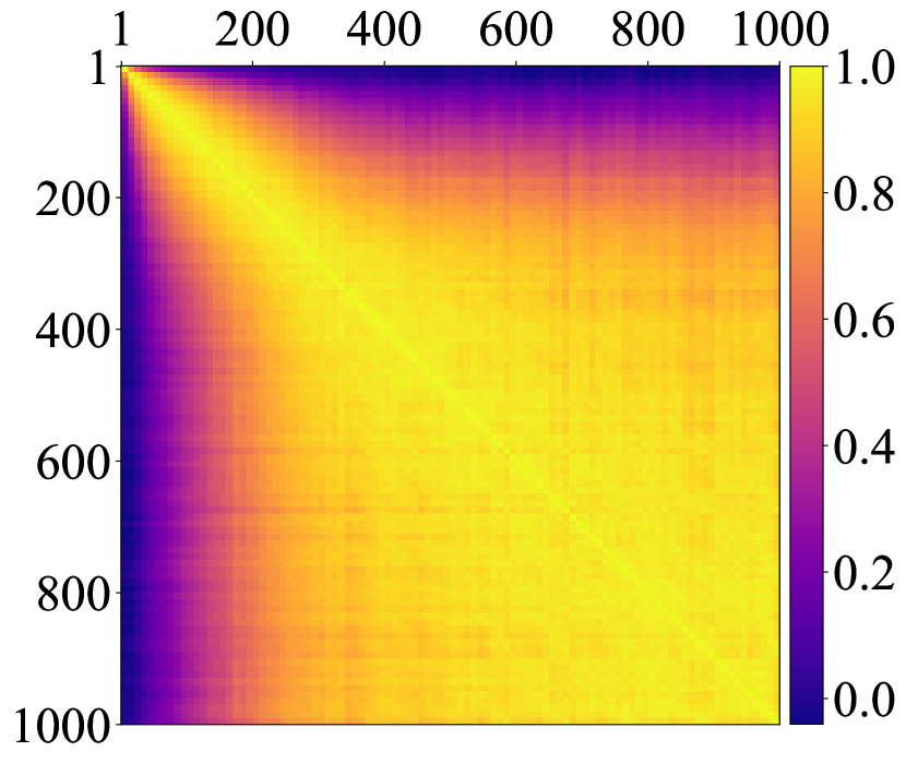
((a)) ADM (timestep $t$)

((b)) ADM (log-SNR)

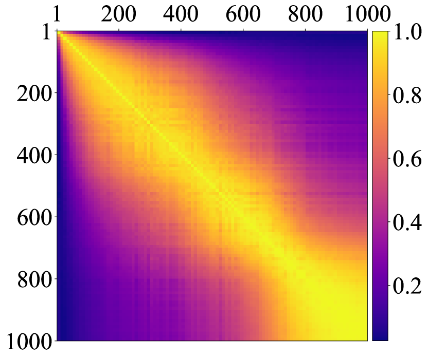
((c)) LDM (timestep $t$)

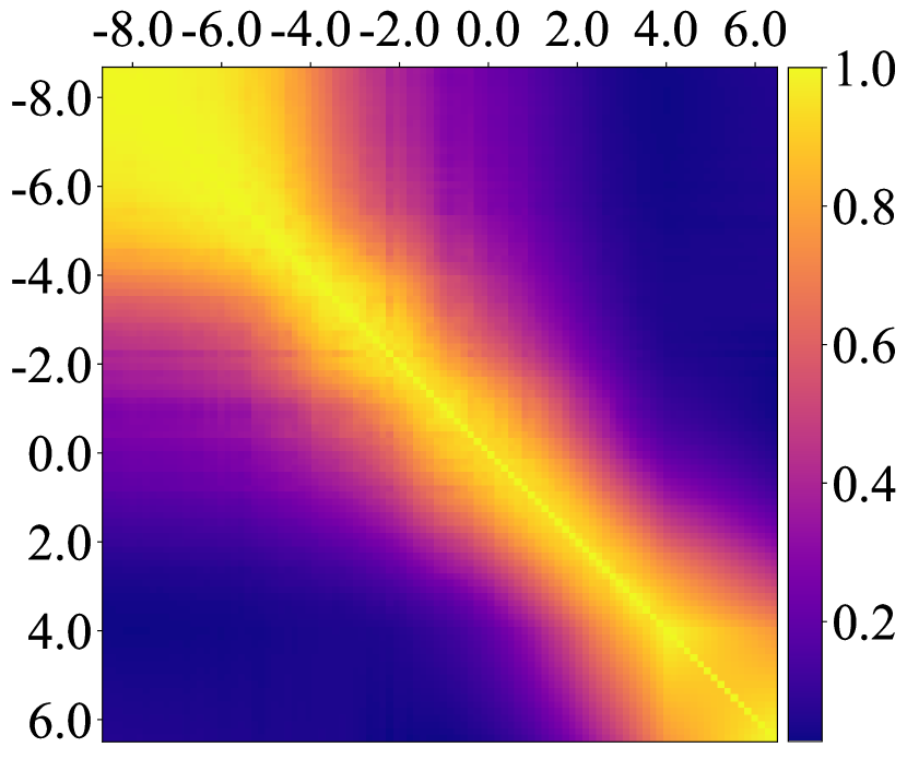
((d)) LDM (log-SNR)

Figure 1: Task affinity scores plotted against timestep and log-SNR axes in ADM and LDM. As the timestep and SNR differences decrease, task affinity increases, implying more aligned gradient directions between denoising tasks and reduced negative impact on their joint training.

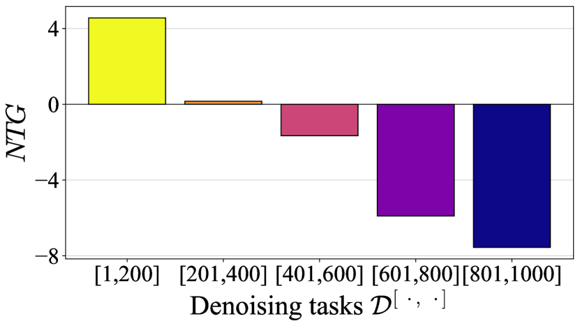
((a)) ADM

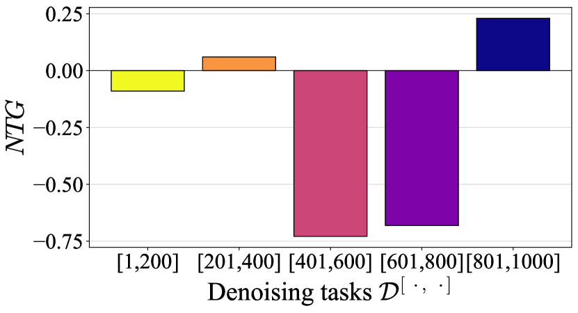
((b)) LDM

Figure 2: Negative transfer gap ($NTG$) with FID score of ADM and LDM for denoising tasks $\mathcal{D}^{[\cdot,\cdot]}$. If $NTG$ is negative, $\mathcal{D}^{[\cdot,\cdot]}$-trained model outperforms the entire denoising tasks-trained model in terms of denoising latent $\{\mathbf{x}_{t}\}_{t\in[\cdot,\cdot]}$, showing the occurrence of negative transfer. Negative transfer occurs in both ADM and LDM.

By considering diffusion training as a form of multi-task learning, we can analyze how the diffusion model learns the denoising task. We experimentally analyze diffusion models with two concepts in multi-task learning: 1) Task affinity [72, 12]: measuring which combinations of denoising tasks may yield a more positive impact on performance. 2) Negative transfer [68, 24, 25, 57, 78, 83]: degradation in denoising tasks caused by multi-task learning. We use a lightweight ADM [8] used in [6] and LDM [56] with FFHQ 256$\times$256 dataset [27] for analyze diffusion models trained on both pixel and latent space.

(O1) Task Affinity Analysis We first analyze how the denoising tasks $\mathcal{D}^{[1,T]}$ relate to each other by measuring task affinities [72, 12]. In particular, we adopt the gradient direction-based task affinity score [78]: for two given tasks $\mathcal{D}^{i}$ and $\mathcal{D}^{j}$, we calculate the pairwise cosine similarity between gradients from each task loss, i.e., $\nabla_{\theta}L_{i}$ and $\nabla_{\theta}L_{j}$, then average the similarities across training iterations. Task affinity score assumes that cooperative (conflicting) tasks produce similar (conflicting) gradient directions, and it has been to correlate with the MTL model’s overall performance [78]. Although there have been attempts to divide diffusion model phases using signal-to-noise ratio [6] and a trace of covariance of training targets [81], we are the first to provide an explicit and fine-grained analysis of task affinities among denoising tasks.

In Fig. 1, we visualize the task affinity scores among denoising tasks, for both ADM and LDM, with both timestep and log-SNR as axes. As can be seen in Fig. 1, task affinity between two tasks $\mathcal{D}^{i},\mathcal{D}^{j}$ is high for neighboring tasks, i.e., $i\approx j$, and decreases smoothly as the difference in SNRs (or timesteps) increases. This suggests that tasks sharing temporal/noise-level proximity can be cooperatively learned without significant conflict. Also, this result hints at the possibility that denoising tasks for vastly different SNRs (distant in timesteps) may potentially be conflicting.

(O2) Negative Transfer Analysis Next, we show that there exist negative transfers among different denoising tasks $\mathcal{D}^{[1,T]}$. Negative transfer refers to a multi-task learner’s performance degradation due to task conflicts, and it can be identified by observing the performance gap between a multi-task learner and specific-task learners. For ease of observation, we group up tasks by intervals, based on the observation (O1) that more neighboring tasks in timesteps have higher task affinity. Specifically, we investigate whether the task group $\mathcal{D}^{[t_{1},t_{2}]}$ suffers negative impacts from the remaining tasks.

To quantify the negative transfer, we follow the procedure: First, we generate samples $\{\tilde{\mathbf{x}}_{0}\}$ using a model trained on all denoising tasks $\mathcal{D}^{[1,T]}$. Next, we repeat the same sampling procedure, except we replace the model with a model trained on $\mathcal{D}^{[t_{1},t_{2}]}$ for the latent $\{\mathbf{x}_{t}\}_{t\in[t_{1},t_{2}]}$; We denote the resulting samples by $\{\tilde{\mathbf{x}}^{[t_{1},t_{2}]}_{0}\}$. If $\{\tilde{\mathbf{x}}^{[t_{1},t_{2}]}_{0}\}$ exhibits superior quality compared to $\{\tilde{\mathbf{x}}_{0}\}$, it indicates that the model trained solely on $\mathcal{D}^{[t_{1},t_{2}]}$ performs better in denoising the latent $\{\mathbf{x}_{t}\}_{t\in[t_{1},t_{2}]}$ than the model trained on the entire denoising task. This suggests that $\mathcal{D}^{[t_{1},t_{2}]}$ suffers from negative transfer by learning other tasks. More formally, given a performance metric $P$, FID [18] in this paper, we define the negative transfer gap:

$$NTG(\mathcal{D}^{[t_{1},t_{2}]}):=P(\{\tilde{\mathbf{x}}^{[t_{1},t_{2}]}_{0}\})-P(\{\tilde{\mathbf{x}}_{0}\}),$$ (3)

where $NTG<0$ indicates that negative transfer occurs. The relationship between the negative transfer gap in previous literature and our negative transfer gap is described in Appendix A.

We visualize the negative transfers among denoising tasks for both lightweight ADM [6, 8] and LDM [56] in Fig. 2. The results indicate that negative transfer occurs in three out of the five considered task groups for both models. Notably, negative transfers often have a significant impact, such as a 7.56 increase in FID for ADM in the worst case. Therefore, we hypothesize that there is room for improving the performance of diffusion models by mitigating negative transfer, which motivates us to leverage well-designed MTL methods for diffusion training.

4 Methodology

In Section 3.2, we make two observations: (O1) Denoising tasks with a larger difference in $t$ and $\text{SNR}(t)$ exhibit lower task affinity, (O2) Negative transfer occurs in diffusion training. Inspired by these observations, we aim to remediate the negative transfer in diffusion by leveraging MTL methods. Although MTL methods are reported effective when there are only a few tasks, they are impractical for diffusion models with a large number of denoising tasks since they require computing per-task gradients or loss at each iteration. In this section, to deal with challenges, we propose a strategy that first groups the denoising tasks as task clusters and then applies the multi-task learning methods by regarding each task cluster as one distinct task.

4.1 Interval Clustering

Here, we first introduce a scheme that groups all denoising tasks $\mathcal{D}^{[1,T]}$ into a small number of task clusters. This is a necessary step for applying well-established MTL methods, for they usually involve computationally expensive subroutines such as computing per-task gradients or loss in each training iteration. Our key idea is to enforce temporal proximity of denoising tasks within task clusters, given our observation (O1) that task affinity is higher for tasks closer in timesteps. Therefore, we assign tasks in pairwise disjoint time intervals.

To obtain the disjoint time intervals, we leverage an interval clustering algorithm [2, 49] that optimizes for various clustering costs. In our case, interval clustering assigns diffusion timesteps $\mathcal{X}=\{1,\dots,T\}$ to $k$ contiguous intervals $I_{1},\dots,I_{k}$, with $\coprod_{i=1}^{k}I_{i}\cap\mathcal{X}=\mathcal{X}$, where $\coprod$ denotes disjoint union. Let $I_{i}=[l_{i},r_{i}]$, $l_{i}\leq r_{i}$ for $i=1,\dots,k$, then we have $l_{1}=1$, and $r_{i}=l_{i+1}-1$ ($i<k$ and $r_{k}=T$). The interval clustering problem is defined as:

$$\min_{l_{1}=1<l_{2}<...<l_{k}}\sum_{i=1}^{k}L_{cluster}(I_{i}\cap\mathcal{X}),\vspace{-0.2cm}$$ (4)

where $L_{cluster}$ denotes the cluster cost.

Generally, it is known that an interval clustering problem of $n$ data points with $k$ intervals can be solved via dynamic programming in $O(n^{2}k\omega(n))$ [49], where $\omega(n)$ is the time required to calculate the one-cluster cost for $L_{cluster}(\mathcal{X})$. If the size of each cluster is too small, it is challenging to learn the corresponding task cluster, so we add constraints on the cluster size for dynamic programming. More details regarding the dynamic programming algorithm can be found in Appendix G.

It remains to design the clustering cost function $L_{cluster}$ to optimize for. We present three clustering cost functions: timestep-based, SNR-based, and gradient-based.

1. Timestep-based Clustering Cost Intuitively, one simple clustering cost is based on timesteps. We use the absolute timestep difference for the clustering objective by setting $L_{cluster}(I_{i}\cap\mathcal{X})=\sum_{t=l_{i}}^{r_{i}}||t_{center}^{i}-t||_{1}^{1}$ in Eq. 4 where $t_{center}^{i}$ denotes the center of interval $I_{i}$. The resulting intervals divide up the timesteps into $k$ uniform intervals.

2. SNR-based Clustering Cost Another useful metric to characterize a denoising task is its signal-to-noise ratio (SNR). Indeed, it has been previously observed that a denoising task encounters perceptually different noisy inputs depending on its SNR [6]. Also, we already observed that denoising tasks with similar SNRs show high task affinity scores (see Section 3.2). Based on this, we use the absolute log-SNR difference for clustering cost. We define the clustering cost as $L_{cluster}(I_{i}\cap\mathcal{X})=\sum_{t=l_{i}}^{r_{i}}||\log\text{SNR}(t_{center}^{i})-\log\text{SNR}(t)||_{1}^{1}$.

3. Gradient-based Clustering Cost Finally, we consider the gradient direction-based task affinity scores (see Section 3.2 for a definition) for clustering cost. Task affinity scores have been used as a metric to group cooperative tasks [78]. Based on a similar intuition, we design a clustering cost as follows: $L_{cluster}(I_{i}\cap\mathcal{X})=-\sum_{t=l_{i}}^{r_{i}}\mathrm{TAS}(t_{center}^{i},t)$ where $\mathrm{TAS}(\cdot)$ is the gradient-based task affinity score. While leveraging more fine-grained information regarding task affinities, this cost function requires computing and storing gradients throughout training.

4.2 Incorporating MTL Methods into Diffusion Model Training

After dividing the denoising tasks into task clusters via interval clustering, we apply multi-task learning methods to the resulting task clusters. As mentioned in Section 2, previous multi-task learning works have tracked down the following causes for negative transfer: (1) conflicting gradient, (2) difference in gradient magnitude, and (3) imbalanced loss scale. In this work, we leverage one representative method that tackles each of the causes mentioned above, namely, (1) PCgrad [83], (2) NashMTL [46], and (3) Uncertainty Weighting [29].

For each training step in diffusion modeling, we compute the noise prediction loss $L^{l}$ for the $l$-th data within the minibatch. As shown in Eq 2, calculating $L^{l}$ involves sampling the timestep $t^{l}$, in which case $L^{l}$ is a loss incurred on the denoising task $\mathcal{D}^{t^{l}}$. We may then assign $L^{i}$ to the appropriate task cluster by considering the corresponding timestep. Subsequently, we may group up the losses as $\{L_{I_{i}}\}_{i=1,\dots,k}$, where $L_{I_{i}}$ is the loss for the $i$-th task cluster. (More details in Appendix C)

1. PCgrad [83] In each iteration, PCgrad projects the gradient of a task onto the normal plane of the gradient of another task when there is a conflict between their gradients. Specifically, PCgrad first calculates the per-interval gradient $\nabla_{\theta}L_{I_{i}}$. Then, if the other interval gradient $\nabla_{\theta}L_{I_{j}}$ for $i\neq j$ has negative cosine similarity with $\nabla_{\theta}L_{I_{i}}$, it projects $\nabla_{\theta}L_{I_{i}}$ onto the normal plane of $\nabla_{\theta}L_{I_{j}}$. PCgrad repeats this process with all of the other interval gradients for all interval gradients, resulting in a projected gradient per interval. Finally, model parameters are updated with the summation of projected gradients.

2. NashMTL [46] In NashMTL, the aggregation of per-task gradients is treated as a bargaining game. It aims to update model parameters with weighted summed gradients $\Delta\theta=\sum_{i=i}^{k}\alpha_{i}\nabla_{\theta}L_{I_{i}}$ by obtaining the Nash bargaining solution to determine $\alpha_{i}$, where $\Delta\theta$ is in the ball of radius $\epsilon$ centered zero, $B_{\epsilon}$. They define the utility function for each player as $u_{i}=\langle\nabla_{\theta}L_{I_{i}},\Delta\theta\rangle$, then the unique Nash bargaining solution can be obtained by $\arg\max_{\Delta\theta\in B_{\epsilon}}\sum_{i}\log(u_{i})$. By denoting $G$ as matrix whose columns contain the gradients $\nabla_{\theta}L_{I_{i}}$, $\alpha\in\mathbb{R}^{k}_{+}$ is the solution to $G^{\intercal}G\alpha=1/\alpha$ where $1/\alpha$ is the element-wise reciprocal. To avoid the optimization to obtain $\alpha$ for each iteration, they update $\alpha$ once every few iterations.

3. Uncertainty Weighting (UW) [29] UW uses task-dependent (homoscedastic) uncertainty to weight task cluster losses. By utilizing observation noise parameter $\sigma_{i}$ for $i$-th task clusters, the total loss function is $\sum_{i}L_{I_{i}}/\sigma^{2}_{i}+\log(\sigma_{i})$. As the noise parameter for the $i$-th task clusters loss $\sigma_{i}$ increases, the weight of $L_{I_{i}}$ decreases, and vice versa. The $\sigma_{i}$ is discouraged from increasing too much by regularizing with $\log(\sigma_{i})$.

5 Experiments

In this section, we demonstrate the efficacy of our proposed method by addressing the negative transfer issue in diffusion training. First, we provide the comparative evaluation in Section 5.1, where our method can boost the quality of generated samples significantly. Next, we compare previous loss weighting methods for diffusion models to UW with interval clustering in Section 5.2, verifying our superior effectiveness to existing methods. Then, we analyze the behavior of adopted MTL methods, which serve to explain the effectiveness of our method in Section 5.3. Finally, we demonstrate that our method can be readily combined with more sophisticated training objectives to boost performance even further in Section 5.4. Extensive information on all our experiments can be found in Appendix E.

5.1 Comparative Evaluation

Experimental Setup Here, we demonstrate that incorporating MTL methods into diffusion training improves the performance of diffusion models. For comparison, we consider unconditional and class-conditional image generation. For unconditional image generation, we used FFHQ [27] and CelebA-HQ [26] datasets, where all images were resized to $256\times 256$. For class-conditional image generation experiments, we employed the ImageNet dataset [7], also resized to $256\times 256$ resolution.

For architecture, we adopt widely recognized architectures for image generation. Specifically, we use the lightweight ADM [6, 8] and LDM [56] for unconditional image generation, while employing DiT-S/2 [52] with classifier-free guidance [19] for class-conditional image generation. We train the model using our method: We consider every possible pair of (1) interval clustering (timestep-, SNR-, and gradient-based) and (2) MTL method (PCgrad, NashMTL, and Uncertainty Weighting (UW)), and report the results. We used $k=5$ in interval clustering throughout experiments.

For evaluation metrics, we use FID [18] and precision [36] for measuring sample quality, and recall [36] for assessing sample diversity and distribution coverage. IS [61] is additionally used for the evaluation metric in the class-conditional image generation setting. Finally, for sample generation, we use DDIM [67] sampler with 50 steps for unconditional generation and DDPM 250 steps for class conditional generation, and all evaluation metrics are calculated using 10k generated samples.

Table 1: Quantitative comparison to vanilla training (Vanilla) on the unconditional generation. Integration of MTL methods using interval clustering consistently improves FID scores and generally enhances precision compared to vanilla training.

Model	Clustering	Method	Dataset
			FFHQ [27]			CelebA-HQ [26]
			FID ($\downarrow$)	Precision ($\uparrow$)	Recall ($\uparrow$)	FID ($\downarrow$)	Precision ($\uparrow$)	Recall ($\uparrow$)
ADM [8, 6]		Vanilla	24.95	0.5427	0.3996	22.27	0.5651	0.4328
	Timestep	PCgrad [83]	22.29	0.5566	0.4027	21.31	0.5610	0.4238
		NashMTL [46]	21.45	0.5510	0.4193	20.58	0.5724	0.4303
		UW [29]	20.78	0.5995	0.3881	17.74	0.6323	0.4023
	SNR	PCgrad [83]	20.60	0.5743	0.4026	20.47	0.5608	0.4298
		NashMTL [46]	23.09	0.5581	0.3971	20.11	0.5733	0.4388
		UW [29]	20.19	0.6297	0.3635	18.54	0.6060	0.4092
	Gradient	PCgrad [83]	23.07	0.5526	0.3962	20.43	0.5777	0.4348
		NashMTL [46]	22.36	0.5507	0.4126	21.18	0.5682	0.4369
		UW [29]	21.38	0.5961	0.3685	18.23	0.6011	0.4130
LDM [56]		Vanila	10.56	0.7198	0.4766	10.61	0.7049	0.4732
	Timestep	PCgrad [83]	9.599	0.7349	0.4845	9.817	0.7076	0.4951
		NashMTL [46]	9.400	0.7296	0.4877	9.247	0.7119	0.4945
		UW [29]	9.386	0.7489	0.4811	9.220	0.7181	0.4939
	SNR	PCgrad [83]	9.715	0.7262	0.4889	9.498	0.7071	0.5024
		NashMTL [46]	10.33	0.7242	0.4710	9.429	0.7062	0.4883
		UW [29]	9.734	0.7494	0.4797	9.030	0.7202	0.4938
	Gradient	PCgrad [83]	9.189	0.7359	0.4904	10.31	0.6954	0.4927
		NashMTL [46]	9.294	0.7234	0.4962	9.740	0.7051	0.5067
		UW [29]	9.439	0.7499	0.4855	9.414	0.7199	0.4952

Comparison in Unconditional Generation As seen in Table 1 our method significantly improves performance upon conventionally trained diffusion models (denoted vanilla in the table). In particular, there is an improvement in FID in all cases, and an improvement in precision scores in all but two cases, which highlights the efficacy of our method. Also, given strong results for both pixel- and latent-space models, we can reasonably infer that our method is generally applicable.

We also observe the distinct characteristics of each multi-task learning method considered. Uncertainty Weighting tends to achieve higher improvements in sample quality compared to PCgrad and NashMTL. Indeed, UW achieves superior FID and Precision for ADM, while excelling in Precision for LDM. However, UW sacrifices distribution coverage in exchange for sample quality, resulting in lower Recall compared to other methods. Meanwhile, NashMTL scores higher in recall and lower in precision compared to other methods, suggesting it has better distribution coverage while sacrificing sample quality. Finally, PCgrad tends to show a balanced performance in terms of precision and recall. We further look into behaviors of different MTL methods in Section 5.3.

Due to space constraints, we provide a comprehensive collection of generated samples in Appendix F. In summary, diffusion models trained with our method produce more realistic and high-fidelity images compared to conventionally trained diffusion models.

Comparison in Class-Conditional Generation

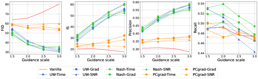
Figure 3: Quantitative comparison to vanilla training (Vanilla) on ImageNet 256$\times$256 dataset with DiT-S/2 architecture and classifier-free guidance. Integration of MTL methods using interval clustering consistently improves FID, IS, and Precision compared to vanilla training.

We illustrate the results of quantitative comparison on class-conditional generation in Fig. 3. The results show that our methods outperform vanilla training in FID, IS, and Precision. In particular, UW and Nash-MTL significantly boost these metrics, showing superior improvement in generation quality. These results further support the generalizability of MTL methods through the interval clustering on class-conditional generation and the transformer-based diffusion model.

5.2 Comparison to Loss Weighting Methods

Table 2: Comparison between MinSNR and ANT-UW. DiT-L/2 is trained on ImageNet.

Method	FID	IS	Precision	Recall
Vanilla	12.59	134.60	0.73	0.49
MinSNR	9.58	179.98	0.78	0.47
ANT-UW	6.17	203.45	0.82	0.47

Table 3: GPU memory usage and runtime comparison on FFHQ dataset in LDM architecture.

Method	GPU memory usage (GB)	# Iterations / Sec
Vanilla	34.126	2.108
PCgrad	28.160	1.523
NashMTL	38.914	2.011
UW	34.350	2.103

Since UW is a loss weighting method, validating the superiority of UW with interval clustering compared to previous loss weighting methods such as P2 [6] and MinSNR [17] highlights the effectiveness of our method. We name UW by incorporating interval clustering as Addressing Negative Transfer (ANT)-UW. We trained DiT-L/2 with MinSNR and UW with $k=5$ on the ImageNet across 400K iterations, using a batch size of 256. All methods are trained by AdamW optimizer [43] with a learning rate of $1e-4$. Table 5.2 shows that ANT-UW dramatically outperforms MinSNR, emphasizing the effectiveness of our method. An essential note is that the computational cost of ANT-UW remains remarkably similar to vanilla training as shown in Section 5.3, ensuring that our enhanced performance does not come at the expense of computational efficiency. Additionally, we refer to the results in [50], showing that our ANT-UW outperforms P2 and MinSNR when DIT-L/2 is trained on the FFHQ dataset.

5.3 Analysis

To provide a better understanding of our method, we present various analysis results here. Specifically, we compare the memory and runtime of MTL methods, analyze the behavior of MTL methods adopted, provide a convergence analysis, and assess the extent to which negative transfer has been addressed.

Memory and Runtime Comparison We first compared the memory usage and runtime between MTL methods and vanilla training for a deeper understanding of their cost. We conducted measurements of memory usage and runtime with $k=5$ on the FFHQ dataset using the LDM architecture and timestep-based clustering, and the results are shown in Table 5.2. PCgrad has a slower speed of 1.523 iterations/second compared to vanilla training, but its GPU memory usage is lower due to the partitioning of minibatch samples. Meanwhile, NashMTL has a runtime of 2.011 iterations/second. Even though NashMTL uses more GPU memory, it has a better runtime than PCgrad because it computes per-interval gradients occasionally. Concurrently, UW shows similar runtime and GPU memory usage as vanilla training, which is attributed to its use of weighted loss and a single backpropagation process.

Behavior of MTL Methods

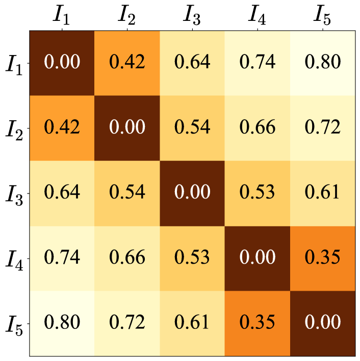
((a)) Average conflict in PCgrad

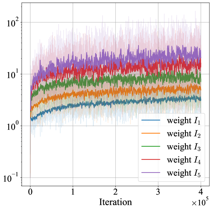
((b)) Gradient weights of NashMTL

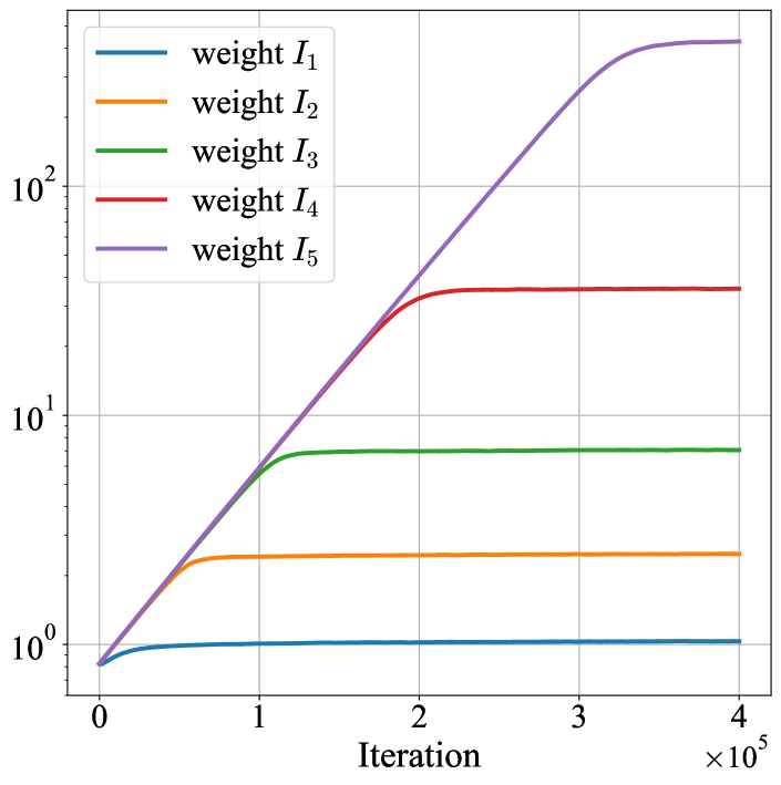
((c)) Loss weight of UW

Figure 4: Behavior of multi-task learning methods across training iterations. (a): With increasing timestep difference, gradient conflicts between task clusters become more frequent in PCgrad. (b) and (c): Both UW and NashMTL allocate higher weights to task clusters that handle noisier inputs.

We analyze the behavior of different multi-task learning methods during training. For PCgrad, we calculate the average number of gradient conflicts between task clusters per iteration. For UW, we visualize the weights allocated to the task cluster losses over training iterations. Finally, for NashMTL, we visualize the weights allocated to per-task-cluster gradients over training iterations. We used LDM trained on FFHQ for our experiments. Although we only report results for time-based interval clustering for conciseness, we note that MTL methods exhibit similar behavior across different clustering methods. Results obtained using other clustering methods can be found in Appendix D.1.

The resulting visualizations are provided in Fig. 4. As depicted in Fig. 4(a), the task pair that shows the most gradient conflicts is $I_{1}$ and $I_{5}$, namely, task clusters apart in timesteps. This result supports our hypothesis that temporally distant denoising tasks may be conflicting, and as seen in Section 5.1, PCgrad seems to mitigate this issue.

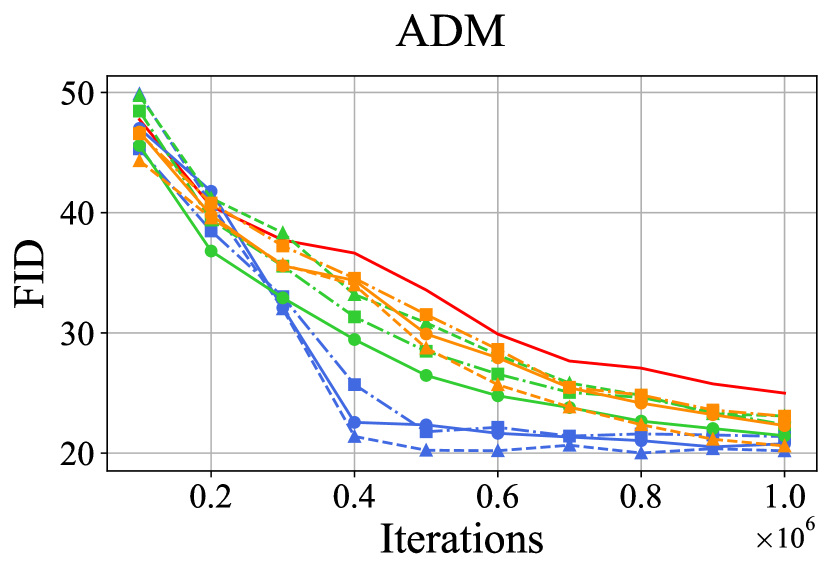
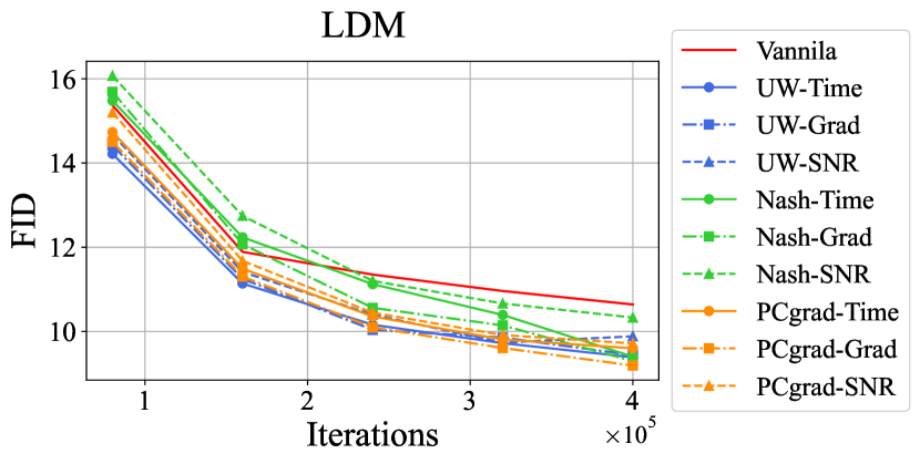
Figure 5: Convergence analysis on FFHQ dataset. Compared to baselines, all methods exhibit fast convergence and achieve good final performance.

Also, as depicted in Fig. 4(b) and  4(b), both UW and NashMTL tend to allocate higher weights to task clusters that handle noisier inputs, namely, $I_{4},I_{5}$. This result suggests that handling noisier inputs may be a difficult task that is underrepresented in conventional diffusion training.

Faster Convergence In Fig. 5, we plot the trajectory of the FID score over training iterations, as observed while training on FFHQ. We can observe that all our methods enjoy faster convergence and better final performance compared to the conventionally trained model. Notably, for pixel space diffusion (ADM), UW converges extremely rapidly, while beating the vanilla method by a large margin. Overall, these results show that our method may not only make diffusion training more effective but also more efficient.

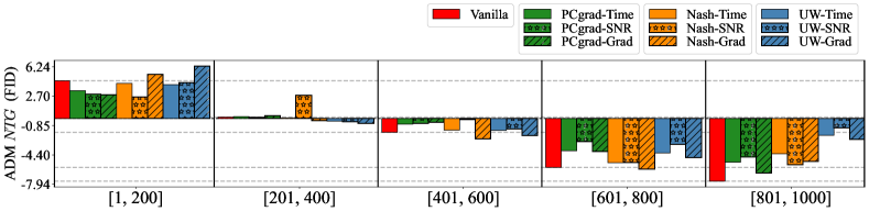
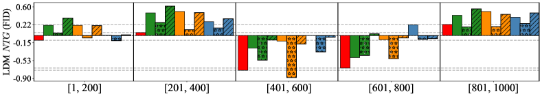
Figure 6: Negative transfer gap (NTG) comparison on the FFHQ dataset. Integration of MTL methods tends to improve the negative transfer gap. Methods that fail to improve NTG in areas where the baseline records low NTG tend to achieve lesser improvements in the baseline.

Reduced Negative Transfer Gap We now demonstrate that our proposed method indeed mitigates the negative transfer gap we observed in Section 3.2. We used the same procedure introduced in Section 3.2 to calculate the negative transfer gap for all methods considered, for the FFHQ dataset.

As shown in Fig. 6 our methods improve upon negative transfer gaps. Specifically, for tasks that exhibit severe negative transfer gaps in the baseline (e.g., [601, 800], [801, 1000] for ADM, and [401, 600], [601, 800] for LDM), our methods mitigate the negative transfer gap for most cases, even practically removing it in certain cases. Another interesting result to note is that models less effective in reducing negative transfer (NashMTL-SNR for LDM and PCgrad-Grad for ADM) indeed show worse FID scores, which supports our hypothesis that resolving negative transfer leads to performance gain. We also note that even the worst-performing methods still beat the vanilla model.

5.4 Combining MTL Methods with Sophisticated Training Objectives

Table 4: Combining our method with P2 on the FFHQ dataset. DDIM 200-step sampler is used.

Type	Method	FID-50k
GAN	PGan [63]	3.39
AR	VQGAN [11]	9.6
Diffusion (LDM)	D2C [65]	13.04
	Vanilla	9.1
	P2	7.21
	P2 + Ours	5.84

Finally, we show that our method is readily applicable on top of more sophisticated training objectives proposed in the literature. Specifically, we train an LDM by applying both UW and PCgrad on top of the P2 objective [6] and evaluate the performance on the FFHQ dataset. We chose UW and PCgrad based on a previous finding that combining the two methods leads to performance gain [41]. Also, we chose the gradient-based clustering method due to its effectiveness for LDM on FFHQ. As seen in Table 4, when combined with P2, our method improves the FID from 7.21 to 5.84.

6 Conclusion

In this work, we studied the problem of better training diffusion models, with the distinction of reducing negative transfer between denoising tasks in a multi-task learning perspective. Our key contribution is to enable the application of existing multi-task learning techniques, such as PCgrad and NashMTL, that were challenging to implement due to the increasing computation costs associated with the number of tasks, by clustering the denoising tasks based on their various task affinity scores. Our experiments validated that the proposed method effectively mitigated negative transfer and improved image generation quality. Overall, our findings contribute to advancing diffusion models. Starting from our work, we believe that addressing and overcoming negative transfer can be the future direction to improve diffusion models.

Appendix

Contents

1. 1 Introduction
2. 2 Related Work
3. 3 Preliminaries and Observation
   1. 3.1 Preliminaries
   2. 3.2 Observation
4. 4 Methodology
   1. 4.1 Interval Clustering
   2. 4.2 Incorporating MTL Methods into Diffusion Model Training
5. 5 Experiments
   1. 5.1 Comparative Evaluation
   2. 5.2 Comparison to Loss Weighting Methods
   3. 5.3 Analysis
   4. 5.4 Combining MTL Methods with Sophisticated Training Objectives
6. 6 Conclusion
7. A Relation to Negative Transfer Gap in Previous Literature
8. B Detailed Experimental Settings for Observational Study
9. C Implementation Details for MTL methods
10. D Additional Experimental Results
    1. D.1 Visualization for the Behavior of MTL Methods with Other Clustering Methods
    2. D.2 Analysis: The Number of Interval Clusters
    3. D.3 Comparison Interval Clustering with Task Grouping Method
    4. D.4 Comparison to Random Loss Weighting and Linear Scalarization
11. E Detailed Experimental Settings in Section 5
    1. E.1 Detailed Settings of Comparative Evaluation and Analysis (Section 5.1 and 5.3)
    2. E.2 Detailed Settings of Comparison to Loss Weighting Methods (Section 5.2)
    3. E.3 Detailed Settings of Combining MTL Methods with Sophisticated Training Objectives (Section 5.4)
12. F Qualitative Results
13. G Dynamic Programming Algorithm for Interval Clustering
14. H Broader Impacts
15. I Limitations

Appendix A Relation to Negative Transfer Gap in Previous Literature

Previous works on transfer and multi-task learning have explored measuring the negative transfer [25, 79, 77]. For the source task $\mathcal{T}_{src}$ and the target task $\mathcal{T}_{tgt}$, the negative transfer can be defined as the phenomenon that the source task negatively transfer to the target task. Denote the model trained on both source and target task as $\Theta(\mathcal{T}_{tgt},\mathcal{T}_{src})$ and the model only trained on the target task as $\Theta(\mathcal{T}_{tgt})$. With performance measure $P$ for the model on $\mathcal{T}_{tgt}$, negative transfer can be quantified by utilizing negative transfer gap ($NTG$):

$$NTG(\mathcal{T}_{tgt},\mathcal{T}_{src})=P(\Theta(\mathcal{T}_{tgt}))-P(\Theta(\mathcal{T}_{tgt},\mathcal{T}_{src})).$$ (5)

For $P$, higher is better, $NTG>0$ indicates that negative transfer occurs, showing that additionally training on $\mathcal{T}_{src}$ negatively affects the learning of $\mathcal{T}_{tgt}$.

In our study of negative transfer in diffusion models, the target task involves denoising tasks within a specific timestep interval as $\mathcal{T}_{tgt}=\mathcal{D}^{[t_{1},t_{2}]}$, while the source task comprises the remaining denoising tasks as $\mathcal{T}_{src}=\mathcal{D}^{[1,T]}\setminus\mathcal{D}^{[t_{1},t_{2}]}$.

However, since a model trained only a subset of entire denoising tasks cannot generate samples properly, we cannot utilize the sample quality metrics (e.g. FID [18]) for $P$ to measure $P(\Theta(\mathcal{T}_{tgt}))$ in Eq. 5 for arbitrary timestep intervals. This is a different point from a typical MTL setting, where the performance of each task can be measured.

Alternatively, we redefine $NTG$ with the difference in sample quality resulting from denoising by different models, $\Theta(\mathcal{T}_{tgt})$ and $\Theta(\mathcal{T}_{tgt},\mathcal{T}_{src})$, in the $[t_{1},t_{2}]$ interval. During the sampling procedure with a model trained on entire denoising tasks, we use $\Theta(\mathcal{T}_{tgt})$ or $\Theta(\mathcal{T}_{tgt},\mathcal{T}_{src})$ in $[t_{1},t_{2}]$. Denote the resulting samples with $\Theta(\mathcal{T}_{tgt},\mathcal{T}_{src})$ as $\{\tilde{x}_{0}\}$ and the resulting samples with $\Theta(\mathcal{T}_{tgt})$ as $\{\tilde{x}_{0}^{[t_{1},t_{2}]}\}$. Then, by comparing the quality of these samples as Eq. 3, we can measure how much the denoising of $[t_{1},t_{2}]$ degrades in terms of sampling quality.

Furthermore, the success of multi-expert denoisers in prior studies [37, 13, 1] suggests the potential existence of negative transfer. By distinctly separating parameters for denoising tasks, they might mitigate this negative transfer, leading to enhanced performance in their generation.

Appendix B Detailed Experimental Settings for Observational Study

In this section, we provide the details on experimental settings in Section 3. The training details and the architectures used are the same as those in Section 5. All experiments are conducted with a single A100 GPU and with FFHQ dataset [27].

For the pixel-space diffusion model, we use the lightweight ADM as same in [6]. It inherits the architecture of ADM [8], but it uses fewer base channels, fewer residual blocks, and a self-attention with a single resolution. Specifically, the model uses one residual block per resolution with 128 base channels and 16$\times$16 self-attention with 64 head channels. A linear schedule with $T=1000$ is used for diffusion scheduling. We referenced the training scripts in the official code for implementation.

For the latent-space diffusion model, we use the LDM architecture as the same settings for FFHQ experiments in [56]. Specifically, an LDM-4-VQ encoder and decoder are used, in which the resolution of latent vectors is reduced by four times compared to the original images and has a vector quantization layer with 8092 codewords. The denoising model has 224 base channels with multipliers for each resolution as 1, 2, 3, 4 and has two residual blocks per resolution. Self-attention with 32 head channels is used for 32, 16, and 8 resolutions. For diffusion scheduling, the linear schedule with $T=1000$ is used. We conducted experiments with the official code. In general, we utilized the pre-trained weights provided by LDM. However, if our retraining results demonstrated superior performance, we reported them.

Task Affinity Analysis

To measure the task affinity score between denoising tasks, we first calculate $\nabla_{\theta}L_{t}$ for $t=1,\dots,T$ every 10K iterations during training. The gradient is calculated with 1000 samples in the training dataset. Then, the pairwise cosine similarity of the gradient is computed and their cosine similarities calculated by every 10K iterations are averaged. Finally, we can plot the average cosine similarity against the timestep axis as in Fig. 1. For plotting them against the log-SNR axis, the values of the axis were adjusted, and the empty parts were filled with linear interpolation.

For ADM and LDM, the pairwise cosine similarity between gradients is calculated during 1M training iterations and 400K training iterations, respectively.

Negative Transfer Analysis

To calculate the negative transfer gap in Eq. 3, we need to additionally train the model on denoising tasks within specific timestep interval $[t_{1},t_{2}]$. Since we plot five intervals [1, 200], [201, 400], [401, 600], [601, 800], and [801, 1000], we trained the model on denoising tasks for each interval. Each model is trained for 600K iterations in ADM and 300K iterations in LDM on the FFHQ dataset. For the model trained on entire denoising tasks, we used the trained model the same as in Section 5.1. ADM is trained on 1M iterations and LDM is trained on 400K iterations. All of these models are trained with the same batch size and learning rate as experiments in Section 5.1 (See Appendix E).

DDIM 50-step sampler [67] was used for the generation. FID is calculated with Clean-FID [51] by setting the entire 70K FFHQ dataset as reference images. Since the official code of Clean-FID supports FID calculation with statistics from these reference images, we used it and reported FID with 10k generated images.

Appendix C Implementation Details for MTL methods

We describe how MTL methods are applied in Section 4.2. To be more self-contained, we hereby present implementation details for MTL methods. For the implementation of MTL methods, we used the official code of LibMTL [39]. NashMTL [46] supports practical speed-up by updating gradient weights $\alpha$ every few iterations, not every iteration. We utilize this by updating $\alpha$ every 25 training iterations.

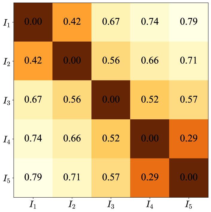
((a)) Average conflict in PCgrad

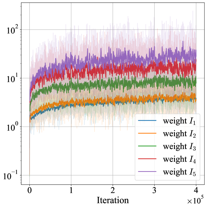
((b)) Gradient weights of NashMTL

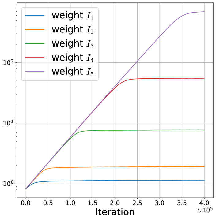
((c)) Loss weight of UW

Figure 7: Behavior of multi-task learning methods through SNR-based interval clustering across training iterations. A similar trend as in Fig. 3 is observed.

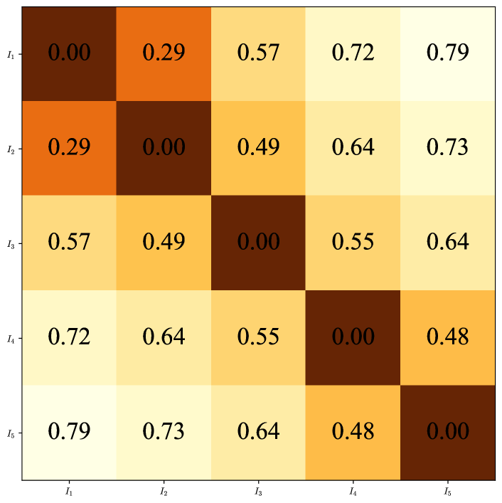
((a)) Average conflict in PCgrad

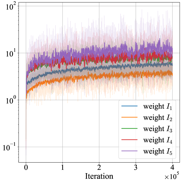
((b)) Gradient weights of NashMTL

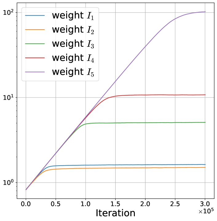
((c)) Loss weight of UW

Figure 8: Behavior of multi-task learning methods through gradient-based interval clustering across training iterations. A similar trend as in Fig. 3 is observed.

Appendix D Additional Experimental Results

We present additional experimental results to supplement the empirical findings presented in Section 5. In Section D.1, we provide visualizations of the behavior of MTL methods with other clustering methods that were not covered in Section 5.3. Furthermore, we examine the impact of our hyperparameter, the number of clusters $k$, in Section D.2. To validate the effectiveness of interval clustering compared to other clustering methods, we present additional results in Section D.3. In Section D.4, we delve deeper into comparing the performance of stronger MTL baselines such as Linear Scalarization (LS) [80, 35] and Random Loss Weighting (RLW) [40] with our proposed approach.

D.1 Visualization for the Behavior of MTL Methods with Other Clustering Methods

Due to space constraints in our main paper, we were unable to include the behavior analysis of MTL methods for SNR-based and gradient-based interval clustering. However, we present these results in Fig. 7 and 8, which show similar trends to the observations depicted in Fig. 4. These findings suggest valuable insights into the behavior of MTL methods, regardless of the clustering objectives.

Firstly, we observed a notable increase in the occurrence of conflicting gradients as the timestep difference between tasks increased. This observation suggests that the temporal distance between denoising tasks plays a crucial role in determining the frequency of conflicting gradients.

Secondly, we noted that both loss and gradient balancing methods assign higher weights to task clusters with higher levels of noise. This finding indicates that these methods allocate more importance to the noisier tasks.

D.2 Analysis: The Number of Interval Clusters

Table 5: FID-10K scores of the LDM trained using a combination of UW and PCgrad methods on the FFHQ dataset while varying the value of $k$. Notably, integrating MTL methods with two clusters significantly improves FID scores. Increasing $k$ from 2 to 5 also enhances FID scores, but further increasing $k$ from 5 to 8 shows similar results.

Clustering	Vanilla	Number of clusters ($k$)
		$k=2$	$k=5$	$k=8$
Timestep	10.56	9.563	9.151	9.083
SNR		9.606	9.410	9.367
Gradient		9.634	9.033	9.145

To understand the impacts of the number of clusters $k$, we conducted experiments by varying $k$ with 2, 5, and 8. We trained a model for timestep-based, SNR-based, and gradient-based clustering with each $k$, resulting in nine trained models. For MTL methods, we used combined methods with UW [29] and PCgrad [83] as in Section 5.4. All training configurations such as learning rate and training iterations are the same as in Section 5.1. We evaluate 10K generated samples from the DDIM 50-step sampler [67] for all methods with the FID score [51, 18].

Table 5 shows the results. Notably, we made an intriguing observation regarding the integration of MTL methods with only two clusters, which resulted in a noteworthy enhancement in FID scores. Additionally, we found that increasing the number of clusters, denoted as $k$, from 2 to 5 also exhibited a positive impact on improving FID scores. However, our findings indicated that further increasing $k$ from 5 to 8 did not yield significant improvements and resulted in similar outcomes. From these results, we conjecture that increasing the number of clusters to greater than five has no significant effect.

D.3 Comparison Interval Clustering with Task Grouping Method

To show the effectiveness of interval clustering methods for denoising task grouping in diffusion models, we compare high-order approximation (HOA)-based grouping methods [72, 12].

For grouping $N$-tasks in deep neural networks, the early attempt [72] established a two-stage procedure: (1) compute MTL performance gain for all task combinations and (2) search best groups for maximizing MTL performance gain across the groups. However, performing (1) requires huge computation since MTL performance gain should be measured for all $2^{N}-1$ combinations. Therefore, they reduce computation by HOA, which utilizes MTL gains on only pairwise task combinations. Also, the HOA scheme is inherited by the following work, task affinity grouping [12], which uses their defined task affinity score instead of MTL gains. Different from these works, our interval clustering aims to group the tasks with interval constraints.

Table 6: Comparison interval clustering and high order approximation-based task grouping. DDIM-50 step sampler is used.

Clustering	FID-10k
HOA	9.873
Interval	9.033

For a fair comparison, we use a pairwise gradient similarity averaged across training iterations between denoising tasks for the objective of HOA-based grouping and interval clustering. In this case, the HOA-based grouping becomes cosine similarity grouping used in [12], and interval clustering becomes gradient-based clustering in our method. However, for HOA-based grouping, a solution of brute force searching with branch-and-bound-like algorithm [72, 12] requires computational complexity of $O(2^{N})$. It incurs enormous costs in diffusion with many denoising tasks. Therefore, we use a beam-search scheme in [68]. We set the number of clusters as 5 for both methods.

We apply the combined method with UW [29] and PCgrad [83] as in Section 5.3 for the resulting clusters from both HOA-based grouping and interval clustering. We trained the model on the FFHQ dataset [27] and used LDM architecture [56]. All training configurations are the same as in Section 5.1. For evaluation metrics, we use FID and its configurations are the same as in Section 5.1.

Table 6 shows the results, indicating that the interval clustering outperforms HOA-based task grouping.

D.4 Comparison to Random Loss Weighting and Linear Scalarization

Table 7: The results of Random Loss Weighting (RLW) and Linear Scalarization (LS) on the FFHQ dataset in ADM architecture.

Clustering	Method	FID	Precision	Recall
-	Vanilla	24.95	0.5427	0.3996
Timestep	RLW	38.06	0.4634	0.3293
	LS	25.34	0.5443	0.3868
SNR	RLW	35.13	0.4675	0.3404
	LS	25.69	0.5369	0.3843
Gradient	RLW	36.19	0.4643	0.3392
	LS	26.12	0.5120	0.3878

Linear Scalarization (LS) [80, 35] and Random Loss Weighting (RLW) [40] can serve as strong baselines for MTL methods. Therefore, validating the superiority of our method compared to theirs can emphasize the necessity of applying sophisticated MTL methods such as UW, PCgrad, and NashMTL. Accordingly, we provide the results of comparative experiments for LS and RLW on the FFHQ dataset using ADM architecture in Table 7. We note that all experimental configuration is the same as in vanilla training in Section 5.1.

As shown in the results, LS achieves slightly worse performance than vanilla training, which suggests that simply re-framing the diffusion training task as an MTL task and applying LS is not enough. Also, RLW achieves much worse performance compared to vanilla training. It appears that the randomness introduced by loss weighting interferes with diffusion training. These results indicate that sophisticated MTL methods are indeed responsible for significant performance gain.

Appendix E Detailed Experimental Settings in Section 5

In this section, we describe the details of experimental settings in Section 5. For validating the effectiveness in both pixel-space and latent-space diffusion models in unconditional generation, we used ADM [8] and LDM [56] as same in our observational study (refer to details of architecture in Appendix B).

E.1 Detailed Settings of Comparative Evaluation and Analysis (Section 5.1 and 5.3)

A single A100 GPU is used for experiments in Section 5.1 and 5.3.

Setups for Unconditional Generation

We trained the models on FFHQ [27] and CelebA-HQ [26] datasets. All training was performed with AdamW optimizer [43] with the learning rate as $1e{-4}$ or $2e{-5}$, and better results were reported. For ADM, we trained 1M iteration with batch size 8 for the FFHQ dataset and trained 400K iterations with batch size 16 for the CelebA-HQ dataset. For LDM, we trained 400K iterations with batch size 30 for both FFHQ and CelebA-HQ datasets. We generate 10K samples with a DDIM-50 step sampler and measure FID [18], Precision [36], and Recall [36] scores. For all evaluation metrics, we use all training data as reference data. FID is calculated with clean-FID [51], and Precision and Recall are computed with publicly available code . All analyses are conducted above trained models.

Setups for Class-Conditional Generation

We trained the DiT-S/2 [52] on ImageNet dataset [7]. All training was performed with the AdamW optimizer [43] with the learning rate of $1e{-4}$ or $2e-5$, and better results were reported. As in DiT [52], we applied the classifier-free guidance [19] and trained 800K iterations with a batch size of 50. All samples are generated by a DDPM 250-step sampler. For evaluation metrics, we follow the evaluation protocol in ADM [8], by using their evaluation code. We used the cosine schedule [47] for noise scheduling and SD-XL VAE [53] for our VAE.

E.2 Detailed Settings of Comparison to Loss Weighting Methods (Section 5.2)

We trained the DiT-L/2 [52] on ImageNet dataset [7]. All training was performed with the AdamW optimizer [43] with the learning rate of $1e{-4}$. As in DiT [52], we applied the classifier-free guidance [19] and trained 400K iterations with a batch size of 256. All samples are generated by a DDPM 250-step sampler and classifier-guidance scale of $1.5$. We used the cosine schedule [47] for noise scheduling. For experiments, we used 8 A100 GPUs.

E.3 Detailed Settings of Combining MTL Methods with Sophisticated Training Objectives (Section 5.4)

We trained three different models: vanilla LDM, vanilla LDM with P2 [6], and vanilla LDM with P2, PCgrad [83], and UW [29] applied simultaneously. All training configurations are the same in Section 5.1 but we use 500K iterations. We generate 50K samples for evaluation with a DDIM 200-step sampler and evaluate FID.

Appendix F Qualitative Results

((a)) Vanila

((b)) PCgrad
- Timestep

((c)) PCgrad
- SNR

((d)) PCgrad
- Gradient

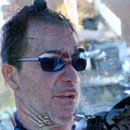
((e)) Nash
- Timestep

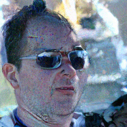
((f)) Nash
- SNR

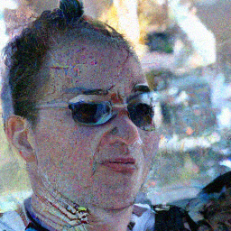
((g)) Nash
- Gradient

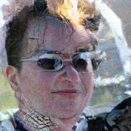
((h)) UW
- Timestep

((i)) UW
- SNR

((j)) UW
- Gradient

Figure 9: Qualitative comparison of ADM trained on the FFHQ dataset.

((a)) Vanila

((b)) PCgrad
- Timestep

((c)) PCgrad
- SNR

((d)) PCgrad
- Gradient

((e)) Nash
- Timestep

((f)) Nash
- SNR

((g)) Nash
- Gradient

((h)) UW
- Timestep

((i)) UW
- SNR

((j)) UW
- Gradient

Figure 10: Qualitative comparison of LDM trained on the FFHQ dataset.

((a)) Vanila

((b)) PCgrad
- Timestep

((c)) PCgrad
- SNR

((d)) PCgrad
- Gradient

((e)) Nash
- Uniform

((f)) Nash
- SNR

((g)) Nash
- Gradient

((h)) UW
- Timestep

((i)) UW
- SNR

((j)) UW
- Gradient

Figure 11: Qualitative comparison of ADM trained on the CelebA-HQ dataset.

((a)) Vanila

((b)) PCgrad
- Timestep

((c)) PCgrad
- SNR

((d)) PCgrad
- Gradient

((e)) Nash
- Timestep

((f)) Nash
- SNR

((g)) Nash
- Gradient

((h)) UW
- Timestep

((i)) UW
- SNR

((j)) UW
- Gradient

Figure 12: Qualitative comparison of LDM trained on the CelebA-HQ dataset.

In this section, we provide qualitative comparison results, which were omitted from the main paper due to space constraints. In Figure 9, 10, 11 and 12, we visualize the generated images by all models that are used for results in Table 1. As shown in the results, we can observe that incorporating MTL methods for diffusion training can improve the quality of generated images. One noteworthy observation is that UW [29] tends to generate higher-quality images compared to NashMTL [46] and PCGrad [83]. This finding aligns with the results observed in Table 1.

Figure 13: Randomly selected images from generated images of LDM with combined methods of UW, PCgrad, and P2 on the FFHQ dataset. DDIM 250-step sampler is used.

Moreover, we plot the randomly selected samples from 50K generated data in Fig. 13. Despite being randomly selected, the majority of the generated images exhibit remarkable fidelity.

Appendix G Dynamic Programming Algorithm for Interval Clustering

In this section, we introduce the algorithm for optimizing the interval cluster and the implementation details. The optimal solution of interval clustering can be found using dynamic programming for a $L_{cluster}$ function [2, 49, 76]. The sub-problem is then defined as finding the minimum cost of clustering $\mathcal{X}_{1,i}=\{1,\dots,i\}$ into $m$ clusters. By saving the minimum cost of clustering $\mathcal{X}_{1,i}=\{1,\dots,i\}$ into $m$ clusters to the matrix $D[i,m]$, the value in $D[T,k]$ represents the minimum clustering costs for the original problem in Eq. 4. For some timestep $m\leq j\leq i$, $D[j-1,m-1]$ must contain the minimum costs for clustering $\mathcal{X}_{1,j-1}$ into $(m-1)$ clusters [49, 76]. This establishes the optimal substructure for dynamic programming, which leads to the recurrence equation as follows:

$$D[i,m]=\min_{m\leq j\leq i}\big{\{}D[j-1,m-1]+L_{cluster}(\mathcal{X}_{j,i})\big{\}},\quad 1\leq i\leq T,\quad 1\leq m\leq k.$$ (6)

To obtain the optimal intervals $l_{1},\dots,l_{k}$, we use $S[i,m]$ to record the argmin solution of Eq. 6. Then, we backtrack the solution in $O(k)$ time from $S[T,k]$ by assigning $l_{m}=S[l_{m+1}-1,m]$ from $m=k$ to $m=1$ by initializing $l_{k}=S[T,k]$.

Interval clustering with SNR-based or gradient-based objectives can produce unbalanced sizes of each interval, which causes unbalanced allocation of task clusters due to randomly sampled timestep $t$. Therefore, we add constraints on the size of each cluster to avoid seriously unbalanced task clusters. To add constraints on the size of each cluster $n_{i}=|I_{i}|=r_{i}-l_{i}+1$ for $i=1,...,k$, we define the lower and upper bounds of it as $m_{I}$ and $M_{I}$ with $m_{I}\leq\frac{n_{i}}{k}\leq M_{I}$. In Eq. 6, the $m$-th cluster (i.e., $\mathcal{X}_{j,i}$) size $n_{m}$ must range from $m_{I}$ to $M_{I}$, yielding $i+1-M_{I}\leq j\leq i+1-m_{I}$. Furthermore, to satisfy the $(m-1)$-clusters constraint, $1+(m-1)m_{I}\leq j$. Finally, Eq. 6 with constraints on the size of the cluster is derived as follows:

$$D[i,m]=\min_{\begin{subarray}{c}\max\{1+(m-1)m_{I},i+1-M_{I}\}\leq j\\ j\leq i+1-m_{I}\end{subarray}}\big{\{}D[j-1,m-1]+L_{cluster}(\mathcal{X}_{j,i})\big{\}},1\leq i\leq T,1\leq m\leq k.$$ (7)

Specifically, we assign $\lfloor\frac{T}{2k}\rfloor$ and $\lceil\frac{3T}{2k}\rceil$ to $m_{I}$ and $M_{I}$, respectively.

Appendix H Broader Impacts

Revisiting Diffusion Models through Multi-Task Learning

Our work revisits diffusion model training from a Multi-Task Learning aspect. We show that negative transfer still occurs in diffusion models and addressing it with MTL methods can improve the diffusion models. Starting from our work, a better understanding of the multi-task learning characteristics in diffusion models can lead to further advancements in diffusion models.

Negative Societal Impacts

Generative models, including diffusion models, have the potential to impact privacy in various ways. For instance, in the context of DeepFake applications, where generative models are used to create realistic synthetic media, the training data plays a critical role in shaping the model’s behavior.

When the training data is biased or contains problematic content, the generative model can inherit these biases and potentially generate harmful or misleading outputs. This highlights the importance of carefully selecting and curating the training data for generative models, particularly when privacy and ethical considerations are at stake.

Appendix I Limitations

Our work has two limitations that can be regarded as future works. Firstly, we have not yet completely resolved the issue of negative transfer in the training of diffusion models as shown in Fig. 5. This indicates that learning entire denoising tasks still causes degradation in certain denoising tasks. By successfully addressing this degradation and enabling the model to harmoniously learn entire denoising tasks, we anticipate significant improvements in the performance of the diffusion model.

Secondly, our study does not delve into the architectural design aspects of multi-task learning methods. While our focus lies on model-agnostic approaches in MTL, it is worthwhile to explore the possibilities of designing appropriate architectures within an MTL framework. Previous works in diffusion models utilize timestep and noise level as input, which can be considered as using task embeddings scheme [73]. By revisiting these aspects, the architecture of the diffusion model can be further advanced in future works.

References

- Balaji et al. [2022] Yogesh Balaji, Seungjun Nah, Xun Huang, Arash Vahdat, Jiaming Song, Karsten Kreis, Miika Aittala, Timo Aila, Samuli Laine, Bryan Catanzaro, et al. ediffi: Text-to-image diffusion models with an ensemble of expert denoisers. arXiv preprint arXiv:2211.01324, 2022.
- Bellman [1973] Richard Bellman. A note on cluster analysis and dynamic programming. Mathematical Biosciences, 18(3-4):311–312, 1973.
- Carlini et al. [2022] Nicholas Carlini, Florian Tramer, Krishnamurthy Dj Dvijotham, Leslie Rice, Mingjie Sun, and J Zico Kolter. (certified!!) adversarial robustness for free! arXiv preprint arXiv:2206.10550, 2022.
- Chen et al. [2018] Zhao Chen, Vijay Badrinarayanan, Chen-Yu Lee, and Andrew Rabinovich. Gradnorm: Gradient normalization for adaptive loss balancing in deep multitask networks. In International conference on machine learning, pages 794–803. PMLR, 2018.
- Chen et al. [2020] Zhao Chen, Jiquan Ngiam, Yanping Huang, Thang Luong, Henrik Kretzschmar, Yuning Chai, and Dragomir Anguelov. Just pick a sign: Optimizing deep multitask models with gradient sign dropout. Advances in Neural Information Processing Systems, 33:2039–2050, 2020.
- Choi et al. [2022] Jooyoung Choi, Jungbeom Lee, Chaehun Shin, Sungwon Kim, Hyunwoo Kim, and Sungroh Yoon. Perception prioritized training of diffusion models. In Proceedings of the IEEE/CVF Conference on Computer Vision and Pattern Recognition, pages 11472–11481, 2022.
- Deng et al. [2009] Jia Deng, Wei Dong, Richard Socher, Li-Jia Li, Kai Li, and Li Fei-Fei. Imagenet: A large-scale hierarchical image database. In 2009 IEEE conference on computer vision and pattern recognition, pages 248–255. Ieee, 2009.
- Dhariwal and Nichol [2021] Prafulla Dhariwal and Alexander Nichol. Diffusion models beat gans on image synthesis. Advances in Neural Information Processing Systems, 34:8780–8794, 2021.
- Dinh et al. [2014] Laurent Dinh, David Krueger, and Yoshua Bengio. Nice: Non-linear independent components estimation. arXiv preprint arXiv:1410.8516, 2014.
- Dinh et al. [2016] Laurent Dinh, Jascha Sohl-Dickstein, and Samy Bengio. Density estimation using real nvp. arXiv preprint arXiv:1605.08803, 2016.
- Esser et al. [2021] Patrick Esser, Robin Rombach, and Bjorn Ommer. Taming transformers for high-resolution image synthesis. In Proceedings of the IEEE/CVF conference on computer vision and pattern recognition, pages 12873–12883, 2021.
- Fifty et al. [2021] Chris Fifty, Ehsan Amid, Zhe Zhao, Tianhe Yu, Rohan Anil, and Chelsea Finn. Efficiently identifying task groupings for multi-task learning. Advances in Neural Information Processing Systems, 34:27503–27516, 2021.
- Go et al. [2023] Hyojun Go, Yunsung Lee, Jin-Young Kim, Seunghyun Lee, Myeongho Jeong, Hyun Seung Lee, and Seungtaek Choi. Towards practical plug-and-play diffusion models. In Proceedings of the IEEE/CVF Conference on Computer Vision and Pattern Recognition, pages 1962–1971, 2023.
- Goodfellow et al. [2020] Ian Goodfellow, Jean Pouget-Abadie, Mehdi Mirza, Bing Xu, David Warde-Farley, Sherjil Ozair, Aaron Courville, and Yoshua Bengio. Generative adversarial networks. Communications of the ACM, 63(11):139–144, 2020.
- Graikos et al. [2022] Alexandros Graikos, Nikolay Malkin, Nebojsa Jojic, and Dimitris Samaras. Diffusion models as plug-and-play priors. Advances in Neural Information Processing Systems, 35:14715–14728, 2022.
- Guo et al. [2018] Michelle Guo, Albert Haque, De-An Huang, Serena Yeung, and Li Fei-Fei. Dynamic task prioritization for multitask learning. In Proceedings of the European conference on computer vision (ECCV), pages 270–287, 2018.
- Hang et al. [2023] Tiankai Hang, Shuyang Gu, Chen Li, Jianmin Bao, Dong Chen, Han Hu, Xin Geng, and Baining Guo. Efficient diffusion training via min-snr weighting strategy. In Proceedings of the IEEE/CVF International Conference on Computer Vision (ICCV), pages 7441–7451, October 2023.
- Heusel et al. [2017] Martin Heusel, Hubert Ramsauer, Thomas Unterthiner, Bernhard Nessler, and Sepp Hochreiter. Gans trained by a two time-scale update rule converge to a local nash equilibrium. Advances in neural information processing systems, 30, 2017.
- Ho and Salimans [2021] Jonathan Ho and Tim Salimans. Classifier-free diffusion guidance. In NeurIPS 2021 Workshop on Deep Generative Models and Downstream Applications, 2021.
- Ho et al. [2020] Jonathan Ho, Ajay Jain, and Pieter Abbeel. Denoising diffusion probabilistic models. Advances in Neural Information Processing Systems, 33:6840–6851, 2020.
- Ho et al. [2022a] Jonathan Ho, William Chan, Chitwan Saharia, Jay Whang, Ruiqi Gao, Alexey Gritsenko, Diederik P Kingma, Ben Poole, Mohammad Norouzi, David J Fleet, et al. Imagen video: High definition video generation with diffusion models. arXiv preprint arXiv:2210.02303, 2022a.
- Ho et al. [2022b] Jonathan Ho, Chitwan Saharia, William Chan, David J Fleet, Mohammad Norouzi, and Tim Salimans. Cascaded diffusion models for high fidelity image generation. Journal of Machine Learning Research, 23(47):1–33, 2022b.
- Ho et al. [2022c] Jonathan Ho, Tim Salimans, Alexey A. Gritsenko, William Chan, Mohammad Norouzi, and David J. Fleet. Video diffusion models. In Alice H. Oh, Alekh Agarwal, Danielle Belgrave, and Kyunghyun Cho, editors, Advances in Neural Information Processing Systems, 2022c.
- Javaloy and Valera [2022] Adrián Javaloy and Isabel Valera. Rotograd: Gradient homogenization in multitask learning. In International Conference on Learning Representations, 2022.
- Jiang et al. [2023] Junguang Jiang, Baixu Chen, Junwei Pan, Ximei Wang, Liu Dapeng, Jie Jiang, and Mingsheng Long. Forkmerge: Overcoming negative transfer in multi-task learning. arXiv preprint arXiv:2301.12618, 2023.
- Karras et al. [2018] Tero Karras, Timo Aila, Samuli Laine, and Jaakko Lehtinen. Progressive growing of GANs for improved quality, stability, and variation. In International Conference on Learning Representations, 2018.
- Karras et al. [2019] Tero Karras, Samuli Laine, and Timo Aila. A style-based generator architecture for generative adversarial networks. In Proceedings of the IEEE/CVF conference on computer vision and pattern recognition, pages 4401–4410, 2019.
- Karras et al. [2022] Tero Karras, Miika Aittala, Timo Aila, and Samuli Laine. Elucidating the design space of diffusion-based generative models. In Alice H. Oh, Alekh Agarwal, Danielle Belgrave, and Kyunghyun Cho, editors, Advances in Neural Information Processing Systems, 2022.
- Kendall et al. [2018] Alex Kendall, Yarin Gal, and Roberto Cipolla. Multi-task learning using uncertainty to weigh losses for scene geometry and semantics. In Proceedings of the IEEE conference on computer vision and pattern recognition, pages 7482–7491, 2018.
- Kim et al. [2022] Gwanghyun Kim, Taesung Kwon, and Jong Chul Ye. Diffusionclip: Text-guided diffusion models for robust image manipulation. In Proceedings of the IEEE/CVF Conference on Computer Vision and Pattern Recognition, pages 2426–2435, 2022.
- Kingma et al. [2021] Diederik Kingma, Tim Salimans, Ben Poole, and Jonathan Ho. Variational diffusion models. Advances in neural information processing systems, 34:21696–21707, 2021.
- Kingma and Welling [2013] Diederik P Kingma and Max Welling. Auto-encoding variational bayes. arXiv preprint arXiv:1312.6114, 2013.
- Kong and Ping [2021] Zhifeng Kong and Wei Ping. On fast sampling of diffusion probabilistic models. In ICML Workshop on Invertible Neural Networks, Normalizing Flows, and Explicit Likelihood Models, 2021.
- Kong et al. [2021] Zhifeng Kong, Wei Ping, Jiaji Huang, Kexin Zhao, and Bryan Catanzaro. Diffwave: A versatile diffusion model for audio synthesis. In International Conference on Learning Representations, 2021.
- Kurin et al. [2022] Vitaly Kurin, Alessandro De Palma, Ilya Kostrikov, Shimon Whiteson, and Pawan K Mudigonda. In defense of the unitary scalarization for deep multi-task learning. Advances in Neural Information Processing Systems, 35:12169–12183, 2022.
- Kynkäänniemi et al. [2019] Tuomas Kynkäänniemi, Tero Karras, Samuli Laine, Jaakko Lehtinen, and Timo Aila. Improved precision and recall metric for assessing generative models. Advances in Neural Information Processing Systems, 32, 2019.
- Lee et al. [2023] Yunsung Lee, Jin-Young Kim, Hyojun Go, Myeongho Jeong, Shinhyeok Oh, and Seungtaek Choi. Multi-architecture multi-expert diffusion models. arXiv preprint arXiv:2306.04990, 2023.
- Li et al. [2022] Xiang Li, John Thickstun, Ishaan Gulrajani, Percy S Liang, and Tatsunori B Hashimoto. Diffusion-lm improves controllable text generation. Advances in Neural Information Processing Systems, 35:4328–4343, 2022.
- Lin and Zhang [2023] Baijiong Lin and Yu Zhang. Libmtl: A python library for deep multi-task learning. Journal of Machine Learning Research, 24:1–7, 2023.
- Lin et al. [2022] Baijiong Lin, Feiyang YE, and Yu Zhang. A closer look at loss weighting in multi-task learning, 2022. URL https://openreview.net/forum?id=OdnNBNIdFul.
- Liu et al. [2021a] Bo Liu, Xingchao Liu, Xiaojie Jin, Peter Stone, and Qiang Liu. Conflict-averse gradient descent for multi-task learning. Advances in Neural Information Processing Systems, 34:18878–18890, 2021a.
- Liu et al. [2021b] Liyang Liu, Yi Li, Zhanghui Kuang, J Xue, Yimin Chen, Wenming Yang, Qingmin Liao, and Wayne Zhang. Towards impartial multi-task learning. International Conference on Learning Representations, 2021b.
- Loshchilov and Hutter [2019] Ilya Loshchilov and Frank Hutter. Decoupled weight decay regularization. In International Conference on Learning Representations, 2019. URL https://openreview.net/forum?id=Bkg6RiCqY7.
- Luo and Hu [2021] Shitong Luo and Wei Hu. Diffusion probabilistic models for 3d point cloud generation. In Proceedings of the IEEE/CVF Conference on Computer Vision and Pattern Recognition, pages 2837–2845, 2021.
- Meng et al. [2022] Chenlin Meng, Yutong He, Yang Song, Jiaming Song, Jiajun Wu, Jun-Yan Zhu, and Stefano Ermon. SDEdit: Guided image synthesis and editing with stochastic differential equations. In International Conference on Learning Representations, 2022.
- Navon et al. [2022] Aviv Navon, Aviv Shamsian, Idan Achituve, Haggai Maron, Kenji Kawaguchi, Gal Chechik, and Ethan Fetaya. Multi-task learning as a bargaining game. In Proceedings of the 39th International Conference on Machine Learning, volume 162 of Proceedings of Machine Learning Research, pages 16428–16446. PMLR, 17–23 Jul 2022. URL https://proceedings.mlr.press/v162/navon22a.html.
- Nichol and Dhariwal [2021] Alexander Quinn Nichol and Prafulla Dhariwal. Improved denoising diffusion probabilistic models. In International Conference on Machine Learning, pages 8162–8171. PMLR, 2021.
- Nichol et al. [2022] Alexander Quinn Nichol, Prafulla Dhariwal, Aditya Ramesh, Pranav Shyam, Pamela Mishkin, Bob Mcgrew, Ilya Sutskever, and Mark Chen. Glide: Towards photorealistic image generation and editing with text-guided diffusion models. In International Conference on Machine Learning, pages 16784–16804. PMLR, 2022.
- Nielsen and Nock [2014] Frank Nielsen and Richard Nock. Optimal interval clustering: Application to bregman clustering and statistical mixture learning. IEEE Signal Processing Letters, 21(10):1289–1292, 2014.
- Park et al. [2023] Byeongjun Park, Sangmin Woo, Hyojun Go, Jin-Young Kim, and Changick Kim. Denoising task routing for diffusion models. arXiv preprint arXiv:2310.07138, 2023.
- Parmar et al. [2022] Gaurav Parmar, Richard Zhang, and Jun-Yan Zhu. On aliased resizing and surprising subtleties in gan evaluation. In Proceedings of the IEEE/CVF Conference on Computer Vision and Pattern Recognition, pages 11410–11420, 2022.
- Peebles and Xie [2023] William Peebles and Saining Xie. Scalable diffusion models with transformers. In Proceedings of the IEEE/CVF International Conference on Computer Vision, pages 4195–4205, 2023.
- Podell et al. [2023] Dustin Podell, Zion English, Kyle Lacey, Andreas Blattmann, Tim Dockhorn, Jonas Müller, Joe Penna, and Robin Rombach. Sdxl: improving latent diffusion models for high-resolution image synthesis. arXiv preprint arXiv:2307.01952, 2023.
- Poole et al. [2022] Ben Poole, Ajay Jain, Jonathan T Barron, and Ben Mildenhall. Dreamfusion: Text-to-3d using 2d diffusion. In The Eleventh International Conference on Learning Representations, 2022.
- Ramesh et al. [2022] Aditya Ramesh, Prafulla Dhariwal, Alex Nichol, Casey Chu, and Mark Chen. Hierarchical text-conditional image generation with clip latents. arXiv preprint arXiv:2204.06125, 2022.
- Rombach et al. [2022] Robin Rombach, Andreas Blattmann, Dominik Lorenz, Patrick Esser, and Björn Ommer. High-resolution image synthesis with latent diffusion models. In Proceedings of the IEEE/CVF Conference on Computer Vision and Pattern Recognition, pages 10684–10695, 2022.
- Ruder [2017] Sebastian Ruder. An overview of multi-task learning in deep neural networks. arXiv preprint arXiv:1706.05098, 2017.
- Saharia et al. [2022a] Chitwan Saharia, William Chan, Saurabh Saxena, Lala Li, Jay Whang, Emily L Denton, Kamyar Ghasemipour, Raphael Gontijo Lopes, Burcu Karagol Ayan, Tim Salimans, et al. Photorealistic text-to-image diffusion models with deep language understanding. Advances in Neural Information Processing Systems, 35:36479–36494, 2022a.
- Saharia et al. [2022b] Chitwan Saharia, Jonathan Ho, William Chan, Tim Salimans, David J Fleet, and Mohammad Norouzi. Image super-resolution via iterative refinement. IEEE Transactions on Pattern Analysis and Machine Intelligence, 2022b.
- Salimans and Ho [2021] Tim Salimans and Jonathan Ho. Progressive distillation for fast sampling of diffusion models. In International Conference on Learning Representations, 2021.
- Salimans et al. [2016a] Tim Salimans, Ian Goodfellow, Wojciech Zaremba, Vicki Cheung, Alec Radford, and Xi Chen. Improved techniques for training gans. Advances in neural information processing systems, 29, 2016a.
- Salimans et al. [2016b] Tim Salimans, Andrej Karpathy, Xi Chen, and Diederik P Kingma. Pixelcnn++: Improving the pixelcnn with discretized logistic mixture likelihood and other modifications. In International Conference on Learning Representations, 2016b.
- Sauer et al. [2021] Axel Sauer, Kashyap Chitta, Jens Müller, and Andreas Geiger. Projected gans converge faster. Advances in Neural Information Processing Systems, 34:17480–17492, 2021.
- Sener and Koltun [2018] Ozan Sener and Vladlen Koltun. Multi-task learning as multi-objective optimization. Advances in neural information processing systems, 31, 2018.
- Sinha et al. [2021] Abhishek Sinha, Jiaming Song, Chenlin Meng, and Stefano Ermon. D2c: Diffusion-decoding models for few-shot conditional generation. Advances in Neural Information Processing Systems, 34:12533–12548, 2021.
- Sohl-Dickstein et al. [2015] Jascha Sohl-Dickstein, Eric Weiss, Niru Maheswaranathan, and Surya Ganguli. Deep unsupervised learning using nonequilibrium thermodynamics. In International Conference on Machine Learning, pages 2256–2265. PMLR, 2015.
- Song et al. [2020] Jiaming Song, Chenlin Meng, and Stefano Ermon. Denoising diffusion implicit models. In International Conference on Learning Representations, 2020.
- Song et al. [2022] Xiaozhuang Song, Shun Zheng, Wei Cao, James Yu, and Jiang Bian. Efficient and effective multi-task grouping via meta learning on task combinations. In Advances in Neural Information Processing Systems, 2022.
- Song and Ermon [2019] Yang Song and Stefano Ermon. Generative modeling by estimating gradients of the data distribution. Advances in neural information processing systems, 32, 2019.
- Song et al. [2021a] Yang Song, Conor Durkan, Iain Murray, and Stefano Ermon. Maximum likelihood training of score-based diffusion models. Advances in Neural Information Processing Systems, 34:1415–1428, 2021a.
- Song et al. [2021b] Yang Song, Jascha Sohl-Dickstein, Diederik P Kingma, Abhishek Kumar, Stefano Ermon, and Ben Poole. Score-based generative modeling through stochastic differential equations. In International Conference on Learning Representations, 2021b.
- Standley et al. [2020] Trevor Standley, Amir Zamir, Dawn Chen, Leonidas Guibas, Jitendra Malik, and Silvio Savarese. Which tasks should be learned together in multi-task learning? In International Conference on Machine Learning, pages 9120–9132. PMLR, 2020.
- Sun et al. [2021] Guolei Sun, Thomas Probst, Danda Pani Paudel, Nikola Popović, Menelaos Kanakis, Jagruti Patel, Dengxin Dai, and Luc Van Gool. Task switching network for multi-task learning. In Proceedings of the IEEE/CVF international conference on computer vision, pages 8291–8300, 2021.
- Vahdat et al. [2021] Arash Vahdat, Karsten Kreis, and Jan Kautz. Score-based generative modeling in latent space. Advances in Neural Information Processing Systems, 34:11287–11302, 2021.
- Van den Oord et al. [2016] Aaron Van den Oord, Nal Kalchbrenner, Lasse Espeholt, Oriol Vinyals, Alex Graves, et al. Conditional image generation with pixelcnn decoders. Advances in neural information processing systems, 29, 2016.
- Wang and Song [2011] Haizhou Wang and Mingzhou Song. Ckmeans. 1d. dp: optimal k-means clustering in one dimension by dynamic programming. The R journal, 3(2):29, 2011.
- Wang et al. [2019] Zirui Wang, Zihang Dai, Barnabás Póczos, and Jaime Carbonell. Characterizing and avoiding negative transfer. In Proceedings of the IEEE/CVF conference on computer vision and pattern recognition, pages 11293–11302, 2019.
- Wang et al. [2021] Zirui Wang, Yulia Tsvetkov, Orhan Firat, and Yuan Cao. Gradient vaccine: Investigating and improving multi-task optimization in massively multilingual models. In International Conference on Learning Representations, 2021.
- Wu et al. [2019] Sen Wu, Hongyang R Zhang, and Christopher Ré. Understanding and improving information transfer in multi-task learning. In International Conference on Learning Representations, 2019.
- Xin et al. [2022] Derrick Xin, Behrooz Ghorbani, Justin Gilmer, Ankush Garg, and Orhan Firat. Do current multi-task optimization methods in deep learning even help? Advances in Neural Information Processing Systems, 35:13597–13609, 2022.
- Xu et al. [2023] Yilun Xu, Shangyuan Tong, and Tommi S. Jaakkola. Stable target field for reduced variance score estimation in diffusion models. In The Eleventh International Conference on Learning Representations, 2023.
- Yang et al. [2023] Xingyi Yang, Daquan Zhou, Jiashi Feng, and Xinchao Wang. Diffusion probabilistic model made slim. In Proceedings of the IEEE/CVF Conference on Computer Vision and Pattern Recognition, pages 22552–22562, 2023.
- Yu et al. [2020] Tianhe Yu, Saurabh Kumar, Abhishek Gupta, Sergey Levine, Karol Hausman, and Chelsea Finn. Gradient surgery for multi-task learning. Advances in Neural Information Processing Systems, 33:5824–5836, 2020.