BOtied: Multi-objective Bayesian optimization with tied multivariate ranks

Abstract

Many scientific and industrial applications require joint optimization of multiple, potentially competing objectives. Multi-objective Bayesian optimization (MOBO) is a sample-efficient framework for identifying Pareto-optimal solutions. We show a natural connection between non-dominated solutions and the highest multivariate rank, which coincides with the outermost level line of the joint cumulative distribution function (CDF). We propose the CDF indicator, a Pareto-compliant metric for evaluating the quality of approximate Pareto sets that complements the popular hypervolume indicator. At the heart of MOBO is the acquisition function, which determines the next candidate to evaluate by navigating the best compromises among the objectives. Multi-objective acquisition functions that rely on box decomposition of the objective space, such as the expected hypervolume improvement (EHVI) and entropy search, scale poorly to a large number of objectives. We propose an acquisition function, called BOtied, based on the CDF indicator. BOtied can be implemented efficiently with copulas, a statistical tool for modeling complex, high-dimensional distributions. We benchmark BOtied against common acquisition functions, including EHVI and random scalarization (ParEGO), in a series of synthetic and real-data experiments. BOtied performs on par with the baselines across datasets and metrics while being computationally efficient.

1 Introduction

Bayesian optimization (BO) has demonstrated promise in a variety of scientific and industrial domains where the goal is to optimize an expensive black-box function using a limited number of potentially noisy function evaluations [1, 2, 3, 4, 5, 6, 7, 8]. In BO, we fit a probabilistic surrogate model on the available observations so far. Based on the model, the acquisition function determines the next candidate to evaluate by balancing exploration (evaluating highly uncertain candidates) with exploitation (evaluating designs believed to maximize the objective). Often, applications call for joint optimization of multiple, potentially competing objectives [9, 10, 11]. Unlike in single-objective settings, a single optimal solution may not exist and we must identify a set of solutions that represents the best compromises among the multiple objectives. The acquisition function in multi-objective Bayesian optimization (MOBO) navigates these trade-offs as it guides the optimization toward regions of interest.

A computationally attractive approach to MOBO scalarizes the objectives with random preference weights [12, 13] and applies a single-objective acquisition function. The distribution of the weights, however, may be insufficient to encourage exploration when there are many objectives with unknown scales. Alternatively, we may address the multiple objectives directly by seeking improvement on a set-based performance metric, such as the hypervolume (HV) indicator [14, 15, 16, 17] or the R2 indicator [18, 19]. Improvement-based acquisition functions are sensitive to the rescaling of the objectives, which may carry drastically different natural units. In particular, computing the HV has time complexity that is super-polynomial in the number of objectives, because it entails computing the volume of an irregularly-shaped polytope [20]. Despite the efficiency improvement achieved by box decomposition algorithms [21, 20], HV computation remains slow when the number of objectives exceeds 4. Another class of acquisition strategies is entropy search, which focuses on maximizing the information gain from the next observation [22, 23, 24, 25, 26, 27]. Computing entropy-based acquisition functions also involves computing high-dimensional definite integrals, this time of an $M$-dimensional multivariate Gaussian, where $M$ is the number of objectives. They are commonly implemented in box decompositions as well, but, are even more costly to evaluate than HV.

Many bona fide MO acquisition functions without scalarization, such as EHVI or entropy searches, involve high-dimensional integrals and scale poorly with increasing numbers of objectives. EHVI and random scalarization are sensitive to non-informative transformations of the objectives, such as rescaling of one objective relative to another or monotonic transformations of individual objectives. To address these challenges, we propose BOtied, a novel acquisition function based on multivariate ranks. We show that BOtied has the desirable property of being invariant to relative rescaling or monotonic transformations of the objectives. While it maintains the multivariate structure of the objective space, its implementation has highly favorable time complexity and we report wall-clock time competitive with random scalarization.

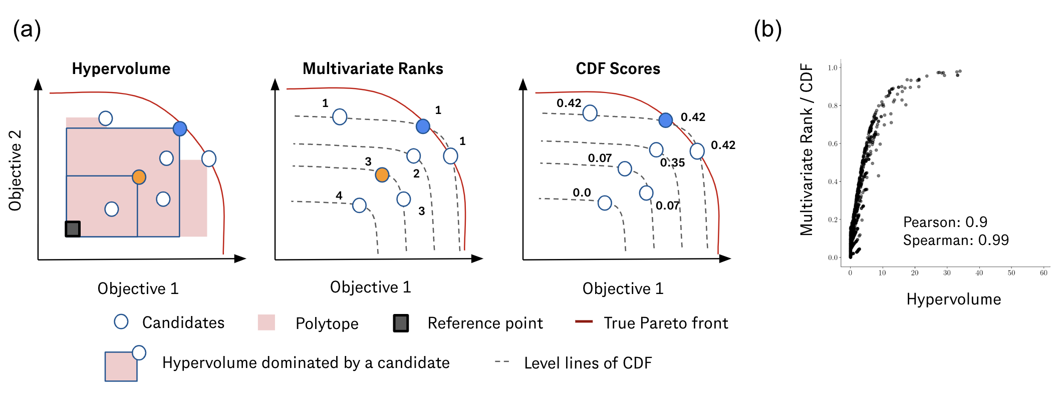
Figure 1: (a) Conceptual summary of BOtied: Here, the blue candidate is predicted to dominate orange with respect to both objectives. The HV indicator is consistent with this ordering; the area of the box bounded by the blue candidate is bigger than that bounded by the orange. Multivariate ranks and CDF scores, used in BOtied, are also more favorable for the blue candidate. (b) The CDF scores closely trace HV.

In Fig. 1(a), we present the intuition behind multivariate ranks. Consider a maximization setup over two objectives where we seek to identify solutions on the true Pareto frontier (red curves), hypothetical and inaccessible to us. Suppose we have many candidates, represented as circular posterior blobs in the objective space, where the posteriors have been inferred from our probabilistic surrogate model. For simplicity, assume the posterior widths (uncertainties) are comparable among the candidates. Let us consider each candidate individually. How do we estimate each candidate’s proximity to the true Pareto frontier? Our surrogate model predicts the candidate shaded in blue to have high values in both objectives and, unbeknownst to us, it happens to lie on the true Pareto front. On the other hand, the candidate shaded in orange is predicted to be strictly dominated by the blue counterpart. The areas of regions bounded from above by the candidates corroborate this ordering, as shown in the leftmost panel; the HV dominated by the blue candidate is bigger than that of the orange. Alternatively, we can compute multivariate ranks of the candidates (middle panel). Consistent with the HV ordering, the blue candidate is ranked higher, at 1, than the orange candidate, at 3. Note that, due to orthogonality, there may be a tie among the candidates.

Ranking in high dimensions is not a trivial task, as there is no natural ordering in Euclidean spaces when $M\geq 2$. To compute multivariate ranks, we propose to use the (joint) cumulative distribution function (CDF) defined as the probability of a sample having greater function value than other candidates, $F_{Y}(y)=P(f(X)\leq y)$, where $y=f(x)$. The gray dashed lines indicate the level lines of the CDF. The level line at $F(\cdot)=1$ is the Pareto frontier estimated by our CDF. As Fig. 1(b) shows, the CDF scores themselves closely trace HV as well.

Motivated by the natural interpretation of multivariate ranks as a multi-objective indicator, we make the following contributions:

• We propose a new Pareto-compliant performance criterion, the CDF indicator (Sec. 2).

• We propose a scalable and robust acquisition function based on the multirank, BOtied (Sec. 3).

• We release a benchmark dataset that explores an ideal case for BOtied ranking, in which we can specify the correct data-generating model when fitting the CDF of the objectives (Sec. 4). The dataset probes particular dependency structures in the objectives and opens the door to incorporating domain knowledge of the objectives.

2 Background

2.1 Bayesian Optimization

Bayesian optimization (BO) is a popular technique for sample-efficient black-box optimization [see 28, 29, for a review]. In a single-objective setting, suppose our objective $f:\mathcal{X}\rightarrow\mathbb{R}$ is a black-box function of the design space $\mathcal{X}$ that is expensive to evaluate. Our goal is to efficiently identify a design $\bm{x}^{\star}\in\mathcal{X}$ maximizing $f$. BO leverages two tools, a probabilistic surrogate model and a utility function, to trade off exploration (evaluating highly uncertain designs) and exploitation (evaluating designs believed to maximize $f$) in a principled manner.

For each iteration $t\in\mathbb{N}$, we have a dataset $\mathcal{D}_{t}=\{(\bm{x}^{(1)},{y}^{(1)}),\cdots,(\bm{x}^{(N_{t})},{y}^{(N_{t})})\}\in\mathscr{D}_{t}$, where each ${y}^{(n)}$ is a noisy observation of $f(\bm{x}^{(n)})$. First, the probabilistic model $\hat{f}:\mathcal{X}\rightarrow\mathbb{R}$ infers the posterior distribution $p(f|\mathcal{D}_{t})$, quantifying the plausibility of surrogate objectives $\hat{f}\in\mathcal{F}$. Next, we introduce a utility function $u:\mathcal{X}\times\mathcal{F}\times\mathscr{D}_{t}:\rightarrow\mathbb{R}$. The acquisition function $a(\bm{x})$ is simply the expected utility of $\bm{x}$ w.r.t. our current belief about $f$,

$$a(\bm{x})=\int u(\bm{x},\hat{f},\mathcal{D}_{t})p(\hat{f}|\mathcal{D}_{t})d\hat{f}.$$ (2.1)

For example, we obtain the expected improvement (EI) acquisition function if we take $u_{\mathrm{EI}}(\bm{x},\hat{f},\mathcal{D})=[\hat{f}(\bm{x})-\max_{(\bm{x}^{\prime},y^{\prime})\in\mathcal{D}}y^{\prime}]_{+},$ where $[\cdot]_{+}=\max(\cdot,0)$ [30, 31]. Often the integral is approximated by Monte Carlo (MC) with posterior samples $\hat{f}^{(j)}\sim p(f|\mathcal{D}_{t})$. We select a maximizer of $a$ as the new design, evaluate $f(a)$, and append the observation to the dataset. The surrogate is then refit on the augmented dataset and the procedure repeats.

2.2 Multi-objective optimization

When there are multiple objectives of interest, a single best design may not exist. Suppose there are $M$ objectives, $f:\mathcal{X}\rightarrow\mathbb{R}^{M}$. The goal of multi-objective BO is to identify the set of Pareto-optimal solutions such that improving one objective within the set leads to worsening another. We say that $\bm{x}$ dominates $\bm{x}^{\prime}$, or ${f}(\bm{x})\succ{f}(\bm{x}^{\prime})$, if $f_{m}(\bm{x})\geq f_{m}(\bm{x}^{\prime})$ for all $m\in\{1,\dotsc,M\}$ and $f_{m}(\bm{x})>f_{m}(\bm{x}^{\prime})$ for some $m$. The set of non-dominated solutions $\mathscr{X}^{*}$ is defined in terms of the Pareto frontier (PF) $\mathcal{P}^{*}$,

$$\mathscr{X}^{\star}=\{\bm{x}:f(\bm{x})\in\mathcal{P}^{\star}\},\hskip 11.38109pt\text{where }\mathcal{P}^{\star}=\{f(\bm{x})\>:\>\bm{x}\in\mathcal{X},\;\nexists\>\bm{x}^{\prime}\in\mathcal{X}\textit{ s.t. }f(\bm{x}^{\prime})\succ f(\bm{x})\}.$$ (2.2)

Multi-objective BO algorithms typically aim to identify a finite subset of $\mathscr{X}^{\star}$, which may be infinite, within a reasonable number of iterations.

Hypervolume

One way to measure the quality of an approximate PF $\mathcal{P}$ is to compute the hypervolume (HV) ${\rm HV}(\mathcal{P}|\bm{r}_{\rm ref})$ of the polytope bounded from above by $\mathcal{P}$ and from below by $\bm{r}_{\mathrm{ref}}$, where $\bm{r}_{\mathrm{ref}}\in\mathbb{R}^{M}$ is a user-specified reference point. More specifically, the HV indicator for a set $A$ is

$$I_{\rm HV}(A)=\int_{\mathbb{R}^{M}}\mathbb{I}[{\bm{r}}_{\rm ref}\preceq{\bm{y}}\preceq A]d{\bm{y}}.$$ (2.3)

We obtain the expected hypervolume improvement (EHVI) acquisition function if we take

$$u_{\mathrm{EHVI}}(\bm{x},\hat{f},\mathcal{D})={\rm HVI}(\mathcal{P}^{\prime},\mathcal{P}|\bm{r}_{\rm ref})=[I_{\rm HV}(\mathcal{P}^{\prime}|\bm{r}_{\rm ref})-I_{\rm HV}(\mathcal{P}|\bm{r}_{\rm ref})]_{+},$$ (2.4)

where $\mathcal{P}^{\prime}=\mathcal{P}\cup\{\hat{f}(\bm{x})\}$ [14, 15].

Noisy observations

In the noiseless setting, the observed baseline PF is the true baseline PF, i.e. $\mathcal{P}_{t}=\{\bm{y}:\bm{y}\in\mathcal{Y}_{t},\>\nexists\>\bm{y}^{\prime}\in\mathcal{Y}_{t}\textit{ s.t. }\bm{y}^{\prime}\succ\bm{y}\}$, where $\mathcal{Y}_{t}\coloneqq\{\bm{y}^{(n)}\}_{n=1}^{N_{t}}$. This does not, however, hold in many practical applications, where measurements carry noise. For instance, given a zero-mean Gaussian measurement process with noise covariance $\Sigma$, the feedback for a candidate $\bm{x}$ is $\bm{y}\sim\mathcal{N}\left({f}(\bm{x}),\Sigma\right)$, not $f(\bm{x})$ itself. The noisy expected hypervolume improvement (NEHVI) acquisition function marginalizes over the surrogate posterior at the previously observed points $\mathcal{X}_{t}=\{\bm{x}^{(n)}\}_{n=1}^{N_{t}}$,

$$u_{\mathrm{NEHVI}}(\bm{x},\hat{f},\mathcal{D})={\rm HVI}(\hat{\mathcal{P}}_{t}^{\prime},\hat{\mathcal{P}}_{t}|\bm{r}_{\rm ref}),$$ (2.5)

where $\hat{\mathcal{P}}_{t}=\{\hat{f}(\bm{x})\>:\>\bm{x}\in\mathcal{X}_{t},\;\nexists\>\bm{x}^{\prime}\in\mathcal{X}_{t}\textit{ s.t. }\hat{f}(\bm{x}^{\prime})\succ\hat{f}(\bm{x})\}$ and $\hat{\mathcal{P}}^{\prime}=\hat{\mathcal{P}}\cup\{\hat{f}(\bm{x})\}$ [17].

3 Multi-objective BO with tied multivariate ranks

In MOBO, it is common to evaluate the quality of an approximate Pareto set ${\mathcal{X}}$ by computing its distance from the optimal Pareto set $\mathcal{X}^{*}$ in the objective space, or $d(f(\mathcal{X}),f(\mathcal{X}^{*}))$. The distance metric $d:2^{\mathcal{Y}}\times 2^{\mathcal{Y}}\rightarrow\mathbb{R}$ quantifies the difference between the sets of objectives, where $2^{\mathcal{Y}}$ is the power set of the objective space $\mathcal{Y}$. Existing work in MOBO mainly focuses on the difference in HV, or HVI. One advantage of HV is its sensitivity to any type of improvement, i.e., whenever an approximation set $A$ dominates another approximation set $B$, then the measure yields a strictly better quality value for the former than for the latter set [32]. Although HV is the most common metric of choice in MOBO, it suffers from sensitivity to scaling and transformation of the objective and scales super-polynomial with the number of objectives, which hinders its practical value.

In the following, the (weak) Pareto-dominance relation is used as a preference relation $\succcurlyeq$ on the search space $X$ indicating that a solution $x$ is at least as good as a solution $y(x\succcurlyeq y)$ if and only if $\forall 1\leq i\leq M:f_{i}(x)\geq f_{i}(y)$. This relation can be canonically extended to sets of solutions where a set $A\subseteq X$ weakly dominates a set $B\subseteq X(A\succcurlyeq B)$ iff $\forall y\in B\ \exists x\in A:x\succcurlyeq y$ [32]. Given the preference relation, we consider the optimization goal to identify a set of solutions that approximates the set of Pareto-optimal solutions and ideally this set is not strictly dominated by any other approximation set.

Since the generalized weak Pareto dominance relation defines only a partial order on $\Omega$, there may be incomparable sets in $\Omega$ which may cause difficulties with respect to search and performance assessment. These difficulties become more serious as $M$ increases (see [33] for details). One way to circumvent this problem is to define a total order on $\Omega$ which guarantees that any two objective vector sets are mutually comparable. To this end, quality indicators have been introduced that assign, in the simplest case, each approximation set a real number, i.e., a (unary) indicator $I$ is a function $I:\Omega\rightarrow\mathbb{R}$ [32]. One important feature an indicator should have is Pareto compliance [33], i.e., it must not contradict the order induced by the Pareto dominance relation.

In particular, this means that whenever $A\succcurlyeq B\land B\nsucceq A$, then the indicator value of A must not be worse than the indicator value of B. A stricter version of compliance would be to require that that the indicator value of A is strictly better than the indicator value of B (if better means a higher indicator value):

$$A\succcurlyeq B\land B\nsucceq A\Rightarrow I(A)>I(B)$$ (3.1)

So far, the hypervolume indicator (and its variations [34]) has been the only known indicator with this property [35].

3.1 CDF indicator

Here we suggest using the cumulative distribution function as an indicator for measuring the quality of Pareto approximations.

Definition 1 (Cumulative distribution function).

The CDF of a real-valued random variable $Y$ is the function given by:

$$F_{Y}(y)=P(Y\leq y)=\int_{-\infty}^{y}p_{Y}(t)dt.$$ (3.2)

i.e. it represents the probability that the r.v. $Y$ takes on a value less than or equal to $y.$

For more then two variables, the joint CDF is given by:

$$F_{Y_{1},\dots,Y_{M}}=P(Y_{1}\leq y_{1},\dots,Y_{M}\leq y_{m})=\int_{(-\infty,\dots,-\infty)}^{(y_{1},\dots,y_{M})}p_{Y}(\mathbf{s})ds$$ (3.3)

Properties of the CDF

Every multivariate CDF is (i) monotonically non-decreasing for each of its variables, (ii) right-continuous in each of its variables and (iii) $0\leq F_{Y_{1},\dots,Y_{M}}(y_{1},\dots,y_{m})\leq 1$. The monotonically non-decreasing property means that $F_{\mathbf{Y}}(a_{1},\dots,a_{M})\geq F_{\mathbf{Y}}(b_{1},\dots,b_{M})$ whenever $a_{1}\geq b_{1},\dots,a_{K}\geq b_{M}$. We leverage these properties to define our CDF indicator.

Definition 2 (CDF Indicator).

The CDF indicator $I_{F}$ is defined as the maximum multivariate rank

$$I_{F_{\mathbf{Y}}}(A):={\rm max}_{y\in A}F_{\mathbf{Y}}(y)$$ (3.4)

where A is an approximation set in $\Omega$.

Next we show that this indicator is compliant with the concept of Pareto dominance.

Theorem 1 (Pareto compliance).

For any arbitrary approximation sets $A\in\Omega$ and $B\in\Omega$, it holds

$$A\succcurlyeq B\land B\nsucceq A\Rightarrow I_{F}(A)\geq I_{F}(B).$$ (3.5)

The proof can be found in Appendix A.

Remark 1.

Note that $I_{F_{\mathbf{Y}}}$ in Eq. 3.4 only depends on the best element in the $F_{\mathbf{Y}}$ rank ordering. One consequence of this is that $I_{F_{\mathbf{Y}}}$ does not discriminate sets with the same best element.

3.2 Estimation of the CDF indicator

Computing a multivariate joint distribution $F_{\mathbf{Y}}$ is a challenging task. A naive approach involves estimating the multivariate density function and then computing the integral, which is computationally intensive. We turn to copulas [36, 37], statistical tool for flexible density estimation in higher dimensions.

Theorem 2 (Sklar’s theorem [38]).

The continuous random vector $Y=(Y_{1},\dots,Y_{M})$ has joint a distribution $F$ and marginal distributions $Y_{1},\dots,F_{M}$ if and only if there exist a unique copula $C$, which is the joint distribution of $U=(U_{1},\dots,U_{M})=F_{1}(Y_{1}),\dots,F_{d}(Y_{M})$.

From Sklar’s theorem, we note that a copula is a multivariate distribution function $C:[0,1]^{M}\rightarrow[0,1]$ that joins (couples) uniform marginal distributions:

$$F(y_{1},\dots,y_{M})=C\left(F_{1}(y_{1}),\dots,F_{d}(y_{M})\right).$$ (3.6)

We notice that by computing the copula function, we also obtain access to the multivariate CDF, and by construction to the multivariate ranking.

It is important to note that, to be able to estimate a copula, we need to transform the variables of interest to uniform marginals. We do so, by the so-called probability integral transform (PIT) of the marginals.

Definition 3 (Probability integral transform).

Probability Integral Transform (PIT) of a random variable $Y$ with distribution $F_{Y}$ is the random variable $U=F_{Y}(y)$, which is uniformly distributed: $U\sim{\rm Unif}([0,1])$.

The benefit of using copulas as estimators for the CDF indicator are three fold: (i) Scalability and flexible estimation in higher dimensional objective spaces, (ii) Scale invariance wrt different objectives, (iii) Invariance Under Monotonic Transformations of the objectives. These three properties suggest that our indicator is more robust than the widely used Hypervolume indicator, as we will empirically show in the following section. Sklar’s theorem, namely the requirement of uniform marginals, immediately implies the following corollary which characterizes the invariance of the CDF indicator to different scales.

Corollary 1 (Scale invariance).

A copula based estimator for the CDF indicator is scale-invariant.

Corollary 2 (Invariance under monotonic transformations).

Let $Y_{1},Y_{2}$ be continuous random variables with copula $C_{Y_{1},Y_{2}}$. If $\alpha,\beta:\mathbb{R}\rightarrow\mathbb{R}$ are strictly increasing functions, then:

$$C_{\alpha(Y_{1}),\beta(Y_{2})}=C_{Y_{1},Y_{2}}$$ (3.7)

where $C_{\alpha(Y_{1}),\beta(Y_{2})}$ is the copula function corresponding to variables $\alpha(Y_{1})$ and $\beta(Y_{2}).$

Corollary 1 follows from the PIT transformation required for copula estimation. The proof for invariance under monotonic transformations based on [39] can be found in Sec. A.2 and, without loss of generality, can be extended to more than two dimensions. We empirically validate the robustness properties of the copula-based estimator in Fig. 2.

11:  Input: Probabilistic surrogate ${\hat{f}}$, initial data $\mathcal{D}_{0}=\{({\bm{x}}_{n},{\bm{y}}_{n})\}_{n=1}^{N_{0}}$, $\mathcal{X}\subset\mathbb{R}^{d},\mathcal{Y}\subset\mathbb{R}^{M}$

22:  Output: Optimal selected subset $\mathcal{D}_{T}$.

33:  Fit the initial surrogate model ${\hat{f}({\bm{x}}_{i})}$ on $\mathcal{D}_{0}$.

44:  for $\{t=1,\dots,T\}$ do

55:     Sample the candidate pool ${\bm{x}}_{1},\cdots,{\bm{x}}_{N}\in\mathcal{X}$

6:     for $\{i=1,\dots,N\}$ do

67:        Evaluate $\hat{f}$ on the candidate pool to obtain the posterior $p(f({\bm{x}}_{i})|\mathcal{D}_{t-1})$

8:        Draw $L$ predictive samples ${\hat{f}}_{i}^{(j)}\sim p(f({\bm{x}}_{i})|\mathcal{D}_{t-1})$, for $j\in[L]$

79:     end for

810:     Obtain uniform marginals $\{u_{i}^{(j)}\}_{i\in[N],j\in[L]}$ from the pooled samples $\{{\hat{f}}_{i}^{(j)}\}_{i\in[N],j\in[L]}$

911:     Version 1: Fit a vine copula $\hat{C}$ on the uniform marginals on the sample level, $\{u_{i}^{(j)}\}_{i\in[N],j\in[L]}$.

Version 2: Fit a vine copula $\hat{C}$ on the mean-aggregated uniform marginals, $\{\frac{1}{L}\sum_{j=1}^{L}u_{i}^{(j)}\}_{i\in[N]}$.

12:     for $\{i=1,\dots,N\}$ do

1013:        Version 1: Compute the expected CDF score $\mathcal{S}({\bm{x}}_{i})=\frac{1}{L}\sum_{j=1}^{L}{\hat{C}}\left(u_{i}^{(j)}\right)$

Version 2: Compute the CDF score of the mean ranks $\mathcal{S}({\bm{x}}_{i})={\hat{C}}\left(\frac{1}{L}\sum_{j=1}^{L}u_{i}^{(j)}\right)$

14:     end for

1115:      $i^{\star}\leftarrow\operatorname*{arg\,max}_{i\in[N]}\mathcal{S}({\bm{x}}_{i})$

16:      $\mathcal{D}_{t}\leftarrow\mathcal{D}_{t-1}\cup\{({\bm{x}}_{i^{\star}},{\bm{y}}_{i^{\star}})\}$

17:  end for

18:  return  $\mathcal{D}_{T}$

Algorithm 1 MOBO with BOtied: a CDF-based acquisition function

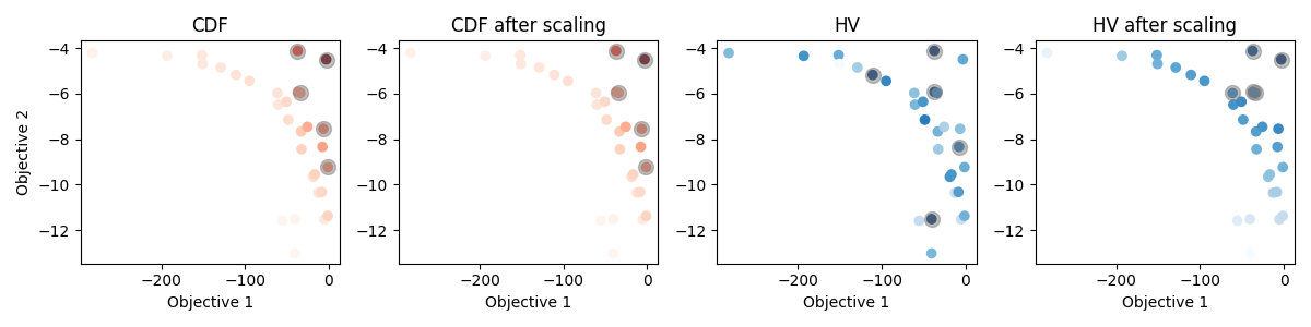
Figure 2: The CDF indicator is more robust to arbitrary rescaling of the objectives than the HV indicator. The color gradient corresponds to value of the indicator for each data point. Gray circles are overlaid on the five selected points with the top indicator scores, where the selection is done in a greedy sequential manner. HV is sensitive to the scales of the objectives.

3.2.1 Estimating high-dimensional CDFs with vine copulas

A copula can be modeled following a parametric family depending on the shape of the dependence structure (e.g., Clayton copula with lower tail dependence, Gumbel copula with upper tail, Gaussian, no tail dependence but full covariance matrix). For additional flexibility and scalability, [40] has proposed vine copulas, a pair-copula construction that allows the factorization of any joint distribution into bivariate copulas. In this construction, the copula estimation problem decomposes into two steps. First, we specify a graphical model, structure called vine consisting of $\frac{M(M-1)}{2}$ number of trees. Second, we choose a parametric or nonparametric estimator for each edge in the tree representing a bivariate copula. In [41] the authors propose efficient algorithms to organize the trees. We add an example decomposition in Appendix A for completeness. For more details on these algorithms and convergence guarantees, please see [40] and references therein.

3.3 CDF-based acquisition function: BOtied

Suppose we fit a CDF on ${\bm{y}}^{(1)},{\bm{y}}^{(2)},\dotsc,{\bm{y}}^{(N_{t})}$, the $N_{t}$ measurements acquired so far. Denote the resulting CDF as ${\hat{F}}(\cdot;\mathcal{D}_{t})$, where we have made explicit the dependence on the dataset up to time $t$. The utility function of our BOtied acquisition function is as follows:

$$u({\bf x},{\hat{f}},\mathcal{D}_{t})={\hat{F}}({\hat{f}}({\bf x});\mathcal{D}_{t}).$$ (3.8)

4 Empirical results

4.1 Experimental Setup

To empirically evaluate the sample efficiency of BOtied, we execute simulated BO rounds on a variety of problems. See Appendix D for more details about our experiments. Our codebase is available in the supplementary material and at anonymous.link.

Metrics We use the HV indicator presented in Sec. 3, the standard evaluation metric for MOBO, as well as our CDF indicator. We rely on efficient algorithms for HV computation based on hyper-cell decomposition as described in [42, 43] and implemented in BoTorch [44].

Baselines We compare BOtied with popular acquisition functions. We assume noisy function evaluations, so implement noisy versions of all the acquisition functions. The baseline acquisition strategies include NEHVI (noisy EHVI) [16] described in Eq. 2.5; NParEGO (noisy ParEGO) [12] which uses random augmented Chebyshev scalarization and noisy expected improvement; and random. For BOtied we have two implementations, v1 and v2, both based on the joint CDF estimation with the only difference being the method of incorporating the variance from the Monte Carlo (MC) predictive posterior samples, either fitting the copula on all of them (v1) or on the means (v2). The algorithms for both versions can be found in algorithm 1.

Datasets As a numerical testbed, we begin with toy test functions commonly used as BO benchmarks: Branin-Currin [45] ($d=2$, $M=2$) and DTLZ [46] ($d=9$, $M\in\{4,6,8\}$). The Penicillin test function [47] ($d=7$, $M=3$) simulates the penicillin yield, time to production, and undesired byproduct for various parameters of the production process. All of these tasks allow for a direct evaluation of $f$.

To emulate a real-world drug design setup, we modify the permeability dataset Caco-2 [48] from the Therapeutics Data Commons database [49, 50]. Permeability is a key property in the absorption, distribution, metabolism, and excretion (ADME) profile of drugs. The Caco-2 dataset consists of 906 drug molecules annotated with experimentally measured rates of passing through a human colon epithelial cancer cell line. We represent each molecule as a concatenation of fingerprint and fragment feature vectors, known as fragprints [51]. We augment the dataset with five additional properties using RDKit [52], including the drug-likeness score QED [53, 54] and topological polar surface area (TPSA) and refer to the resulting $M=6$ dataset as Caco-2+. In many cases, subsets of these properties (e.g., permeability and TPSA) will be inversely correlated and thus compete with one another during optimization. In late-state drug optimization, the trade-offs become more dramatic and as more properties are added [55]. Demonstrating effective sampling of Pareto-optimal solutions in this setting is thus of great value.

4.2 Copulas in BO

In the low-data regime, empirical Pareto frontiers tend to be noisy. When we have access to domain knowledge about the objectives, we can use it to construct a model-based Pareto frontier using vine copulas. This section describes how to incorporate (1) the known correlations among the objectives to specify the tree structure (vine) and (2) the pairwise joint distributions (including the tail behavior), approximately estimated from domain knowledge, when specifying the copula models. The advantages of integrating copula-based estimators for our metric and acquisition function are threefold: (i) scalability from the convenient pair copula construction of vines, (ii) robustness wrt marginal scales and transformations thanks to inherent copula properties 1 and 2, and (iii) domain-aware copula structures from the explicit encoding of dependencies in the vine copula matrix, including choice of dependence type (e.g., low or high tail dependence).

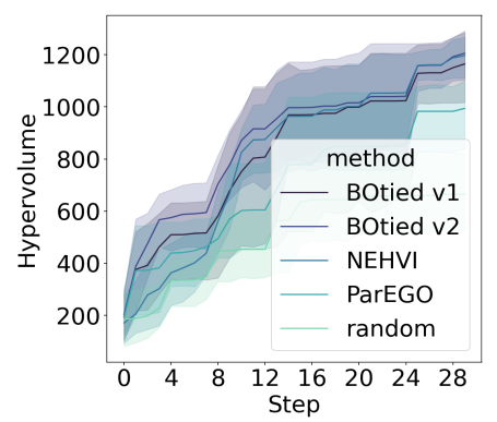
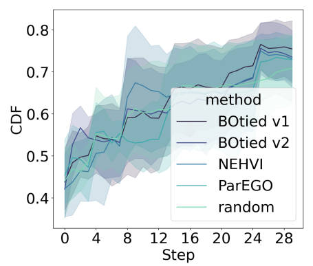
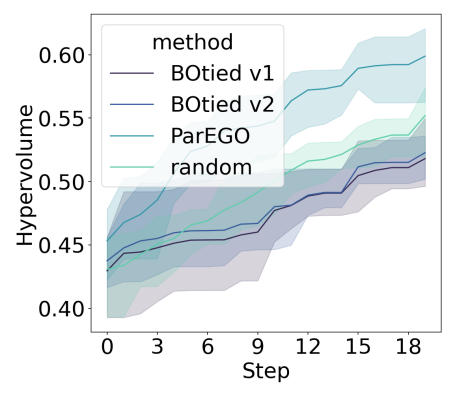
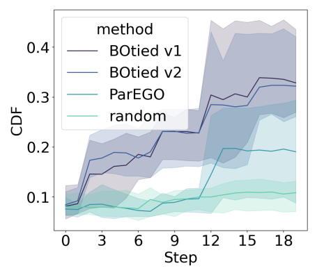
Figure 3: HV and CDF over simulated BO iterations for Branin-Currin ($d=2,M=2$) and DTLZ ($d=9,M=6$) test functions.

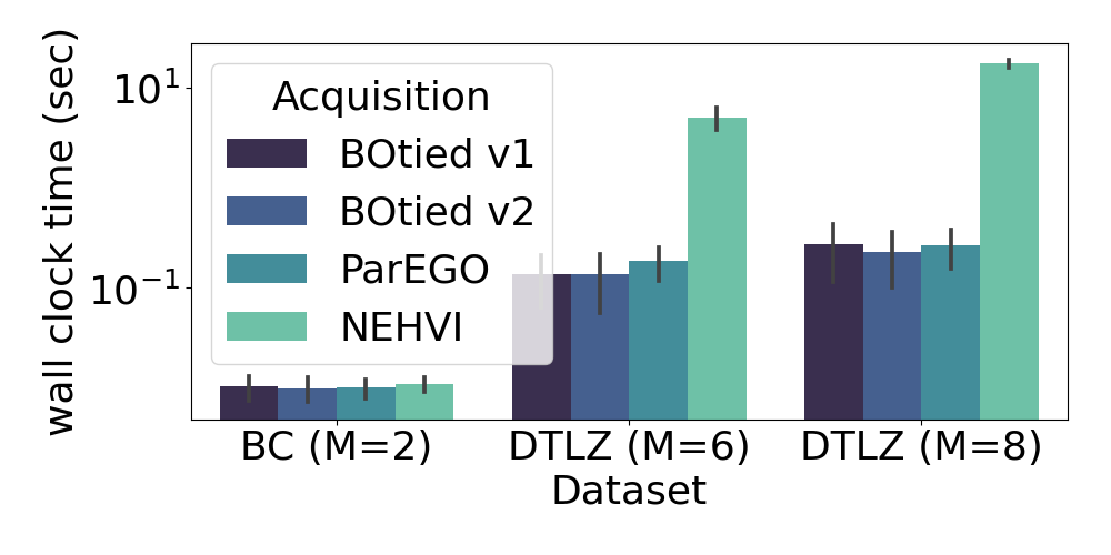
Figure 4: Wall clock time per single call of acquisition function.

Fig. 5 illustrates the use of copulas in the context of optimizing multiple objectives in drug discovery, where data tends to be sparse. In panel (a) we see that, thanks to the separate estimation of marginals and dependence structure, different marginal distributions have the same Pareto front in the PIT space, in which we evaluate our CDF scores. Hence, with copula based estimators, we can guarantee robustness without any overhead for scalarization or standardization of the data as required by counterparts. In panel (b) we show how we can encode domain knowledge of the interplay between different molecular properties in the Caco2+ dataset. Namely, permeability is often highly correlated with ClogP and TPSA, with positive and negative correlation, respectively, which is even more notable at the tails of the data (see panel (a) and Appendix). Such dependence can be encoded in the vine copula structure and in the choice of copula family for each pair. For example, a rotated Clayton copula was imposed so that the tail dependence between TPSA and permeability is preserved.

New flexible test function

We design a dataset named CopulaBC to explore an ideal case for BOtied ranking, in which we do not incur error from specifying an incorrect CDF model. The objectives follow a known joint distribution, recoverable using the true data-generating model for the marginals and for the copula. For particular copula families, this dataset also enables analyses of the dependency structure of the objectives out to the tails. We set $d=2$, $M=2$ for simplicity but a higher dimensional dataset can be generated with an analogous approach. See Appendix B for details.

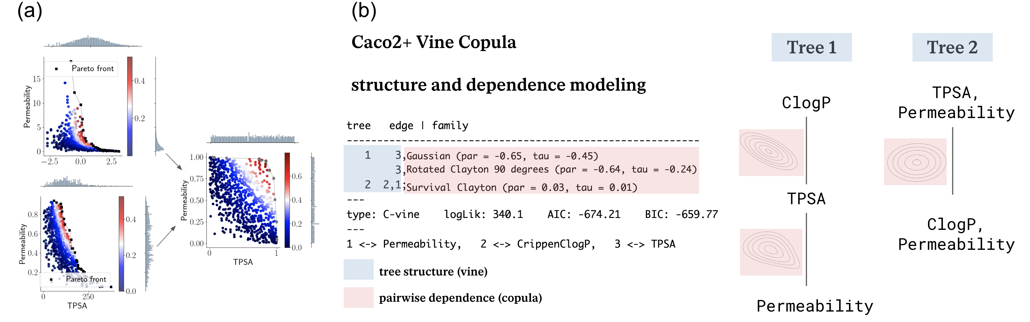
Figure 5: (a). Regardless of the distributions of the marginals, the CDF score from a copula is the same. (b) An example of explicitly encoding domain knowledge in a BO procedure by imposing the in blue tree structure (specifying the matrix representation of the vine) and in pink selection of pairwise dependencies (choice of parametric/non-parametric family).

4.3 Results and discussion

We compare the performance of BOtied with baselines in terms of both the HV and the CDF indicators Table 1. Although there is no single best method across all the datasets, the best numbers are consistently achieved by either BOtied v1 or v2 with NParEGO being a close competitor. The NEHVI performance visibly degrades as $M$ increases and it becomes increasingly slow. In addition to being on par with commonly used acquisition functions, BOtied is significantly faster than NEHVI Fig. 4. There are two main benefits to using the CDF metric rather than HV for evaluation. First, the CDF is bounded between 0 and 1, with scores close to 1 corresponding to the discovered solutions closest to our approximate Pareto front. Unlike with HV, for which the scales do not carry information about the internal ordering, the CDF values have an interpretable scale. Second, applying the CDF metric for different tasks (datasets), we can easily assess how the acquisition performance varies with the specifics of the data.

Limitations

There is a trade-off between the flexibility and complexity when fitting a copula model and by construction, computing BOtied’s score. As the number of objectives grow so does the number of choices that need to be made (pair copulas, parameters etc). For efficiency, in experiments we always pre-select the copula family (Gaussian or KDE), which reduces time complexity without impacting BOtied’s performance.

Table 1: Mean and standard deviation for HV, computed in the original units, and CDF indicators across synthetic datasets. Higher is better and best per column is marked in bold.

	BC (M=2)		DTLZ (M=4)		DTLZ (M=6)		DTLZ (M=8)
	CDF	HV	CDF	HV	CDF	HV	CDF	HV
BOtied v1	0.76 (0.06)	1164.43 (174.37)	0.2 (0.1)	0.42 (0.03)	0.33 (0.09)	0.52 (0.02)	0.2 (0.08)	0.93 (0.02)
BOtied v2	0.74 (0.08)	1205.3 (120.46)	0.24 (0.2)	0.45 (0.05)	0.32 (0.08)	0.58 (0.03)	0.19 (0.1)	0.91 (0.03)
NParEGO	0.73 (0.09)	993.31 (178.16)	0.20 (0.07)	0.4 (0.03)	0.29 (0.03)	0.69 (0.02)	0.13 (0.07)	1.05 (0.02)
NEHVI	0.73 (0.07)	1196.37 (98.72)	0.21 (0.02)	0.44 (0.04)	–	–	–	–
Random	0.71 (0.11)	1204.99 (69.34)	0.1 (0.05)	0.22 (0.03)	0.10 (0.03)	0.55 (0.02)	0.13 (0.07)	0.96 (0.02)
	Caco2+ (M=3)		Penicillin (M=3)		CopulaBC (M=2)
	CDF	HV	CDF	HV	CDF	HV
BOtied v1	0.58 (0.06)	11645.63 (629.0)	0.48 (0.02)	319688.6 (17906.2)	0.9 (0.03)	1.08 (0.03)
BOtied v2	0.60 (0.06)	11208.57(882.21)	0.49 (0.02)	318687.7 (17906.2)	0.9 (0.01)	1.09 (0.02)
NParEGO	0.56 (0.05)	12716.2 (670.12)	0.28 (0.09)	332203.6 (15701.52)	0.87 (0.01)	1.1 (0.01)
NEHVI	0.54 (0.06)	13224.7 (274.6)	0.24 (0.05)	318748.9 (2868.64)	0.88 (0.02)	1.1 (0.01)
Random	0.57 (0.07)	11425.6 (882.4)	0.32 (0.02)	327327.9 (17036)	0.88 (0.02)	1.08 (0.01)

5 Conclusion

We introduce a new perspective on MOBO by leveraging multivariate ranks computed with CDF scores. We propose a new Pareto-compliant CDF indicator with an efficient implementation using copulas as well as a CDF-based acquisition function. We have demonstrated our CDF-based estimation of the non-dominated regions allows for greater flexibility, robustness, and scalability compared to existing acquisition functions. This method is general and lends itself to a number of immediate extensions. First, we can encode dependencies between objectives, estimated from domain knowledge, into the graphical vine model. Second, we can accommodate discrete-valued objectives. Finally, as many applications carry noise in the input as well as the function of interest, accounting for input noise through the established connection between copulas and multivariate value-at-risk (MVaR) estimation will be of great practical interest. Whereas we have focused on selecting candidates from a fixed library, the computation of our acquisition function is differentiable and admits gradient-based sampling from the input space.

Appendix A Properties of the CDF indicator

A.1 Theorem 1: Pareto compliance of the CDF indicator

We state Theorem 1 again and provide the proof here.

Theorem 1: For any arbitrary approximation sets $A\in\mathcal{X}$ and $B\in\mathcal{X}$ where $\mathcal{X}\subset\mathbb{R}^{d}$, the following holds:

$$A\succcurlyeq B\land B\nsucceq A\Rightarrow I_{F}(A)\geq I_{F}(B).$$

Proof.

If we have $A\succcurlyeq B\land B\nsucceq A$, then the following two conditions hold: $\forall{\bm{x}}^{\prime}\in B\ \exists{\bm{x}}\in A:{\bm{x}}\succcurlyeq{\bm{x}}^{\prime}$ and $\exists\mathbf{x}\in A\ s.t.\ \nexists{\bm{x}}^{\prime}\in B:{\bm{x}}^{\prime}\succcurlyeq\mathbf{x}$. Recall that the weak Pareto dominance $\mathbf{x}\succcurlyeq\mathbf{x}^{\prime}$ implies that $\forall i\in[M]:f_{i}({\bm{x}})\geq f_{i}({\bm{x}}^{\prime})$. From the definition and fundamental property of the CDF being a monotonic non-decreasing function, it follows that $\forall i\in[M]:f_{i}({\bm{x}})\geq f_{i}({\bm{x}}^{\prime})\Rightarrow F_{\mathbf{Y}}({\bm{x}})\geq F_{\mathbf{Y}}({\bm{x}}^{\prime})$.

Define the set of non-dominated solutions in $B$, $\mathcal{P}_{B}\coloneqq\{{\bm{x}}\in B,\forall{\bm{x}}^{\prime}\in B:{\bm{x}}\succeq{\bm{x}}^{\prime}\}$. Note that $I_{F}(B)=I_{F}(\mathcal{P}_{B})=I_{F}(\{{\bm{z}}\})$ for any ${\bm{z}}\in\mathcal{P}_{B}$. Now let ${\bm{x}}_{B}\in\mathcal{P}_{B}$. There is ${\bm{x}}_{A}\in A$ such that ${\bm{x}}_{A}\succeq{\bm{x}}_{B}$, and we have that $F_{\mathbf{Y}}({\bm{x}}_{A})\geq F_{\mathbf{Y}}({\bm{x}}_{B})$. By definition, $I_{F}(A)\geq I_{F}(\{{\bm{x}}_{A}\})$ so we have $I_{F}(A)\geq I_{F}(\{{\bm{x}}_{A}\})\geq I_{F}(\{{\bm{x}}_{B}\})=I_{F}(B)$ as desired. ∎

A.2 Corollary 2: Invariance under monotonic transformations

This proof closely follows the one in [39].

Corollary 2: Let $Y_{1},Y_{2}$ be continuous random variables with copula $C_{Y_{1},Y_{2}}$. If $\alpha,\beta:\mathbb{R}\rightarrow\mathbb{R}$ are strictly increasing functions, then:

$$C_{\alpha(Y_{1}),\beta(Y_{2})}=C_{Y_{1},Y_{2}}$$ (A.1)

where $C_{\alpha(Y_{1}),\beta(Y_{2})}$ is the copula function corresponding to variables $\alpha(Y_{1})$ and $\beta(Y_{2}).$

Proof.

We first note that for the distribution function of $\alpha(Y_{1})$ it holds that

$$F_{\alpha(Y_{1})}=P(\alpha(Y_{1})\leq y_{1})=P(Y_{1}\leq\alpha^{-1}(y_{1}))=F_{Y_{1}}(\alpha^{-1}(y_{1}))$$ (A.2)

and analogously,

$$F_{\beta}(Y_{1})(y_{1})=F_{Y_{1}}(\beta^{-1}(y_{1}))$$ (A.3)

From Sklar’s theorem, we have that for all $y_{1},y_{2}\in\mathbb{R}$

$$C_{\alpha(Y_{1})\beta(Y_{2})}(F_{\alpha(Y_{1})}(y_{1}),F_{\beta(Y_{2})}(y_{2})) =F_{\alpha(Y_{1})\beta(Y_{2})}(y_{1},y_{2})$$

$$=P(\alpha(Y_{1})\leq y_{1},\beta(Y_{2})\leq y_{2})$$

$$=P(Y_{1}\leq\alpha^{-1}(y_{1}),Y_{2}\leq\beta^{-1}(y_{2}))$$

$$=F_{Y_{1},Y_{2}}(\alpha^{-1}(y_{1}),\beta^{-1}(y_{2})))$$

$$=C_{Y_{1},Y_{2}}(F_{Y_{1}}(\alpha^{-1}(y_{1})),F_{Y_{2}}(\beta^{-1}(y_{2})))$$

$$=C_{Y_{1},Y_{2}}(F_{\alpha(Y_{1})}(y_{1}),F_{\beta(Y_{2})}(y_{2}))$$

Equalities one and five follow from Sklar’s theorem. In the third equality we make use of fact that $\alpha$ and $\beta$ are increasing functions. The last equality follows from Sec. A.2 and Sec. A.2. ∎

Appendix B CopulaBC test function

We design and release a dataset named CopulaBC for MOBO benchmarking. CopulaBC explores an ideal case for BOtied ranking, in which we do not incur error from specifying an incorrect CDF model. The objectives follow a known joint distribution. The generation process is as follows:

$$U \sim C$$ (B.1)

$$\forall i\in[M]:Y_{i} =F_{i}^{-1}(U_{i})$$ (B.2)

$$X =g^{-1}(Y),$$ (B.3)

where $C$ is the assigned copula model and $g$ is the function mapping inputs in $\mathcal{X}\subset\mathbb{R}^{d}$ to outputs in $\mathbb{R}^{M}$. In words, we first sample the uniform marginals in $\mathbb{R}^{M}$ from a copula model of choice in Eq. B.1. We may impose the correlation structure of interest in the copula model; for instance, we may assign a flipped Clayton copula if we want to emulate a heavy right tail behavior, as is common in biophysical properties [10]. The uniform marginals are then converted into the observation space via the marginal quantile functions $F_{i}^{-1}$ for each dimension $i\in[M]$. Lastly, the resulting $Y\in\mathbb{R}^{M}$ are mapped back to the input $X\in\mathcal{X}\subset\mathbb{R}^{d}$ via the inverse model $g^{-1}$.

For CopulaBC, we use the flipped Clayton copula with one parameter for $C$. Choosing within the Archimedean copula family offers the advantage of analytic expressions of the Pareto front, as their level lines admit an analytic form. We specifically opt for the Branin-Currin function for $g^{-1}$ (hence the “BC” in the name CopulaBC), but other functions with bigger $d$ and $M$ may be used as long as the support of $F_{i}$ is consistent with the image of $g$ (i.e., the space of $Y$ is matched between $F_{i}$ and $g$). Because we restrict the domain of Branin-Currin (the image of our $g$) to $[0,1]^{d}$, we chose $F_{i}(\cdot)={\rm Beta}(\cdot;\alpha=2,\beta=2)$ for all $i\in[M]$. We can also choose from a number of parametric families (e.g., exponential, Gaussian, Student’s t) because, thanks to the nature of copulas, the marginals have no impact on the dependence structure.

Our copula dataset ensures that the objective $Y$ follows a distribution that can be fit easily using the true data-generating model for the marginals and for the copula (e.g., beta and Clayton, respectively, for CopulaBC). However, this copula-based test function is general and allows for “mimicking” a variety of scenarios in stress tests or ablation studies, depending on the application. A practitioner can control for the following:

1. choice of dependence structure, high or low tail dependence (very common in finance for example)

2. choice of distribution $F_{i}$ for each of the marginals (for example, drug-related properties often follow zero-inflated distributions with upper tails)

3. choice of the vine structure; as illustrated in Fig. 5, we can decide on the pairwise factorization and enforce dependencies between properties via the vine copula matrix.

Appendix C (Vine) copula overview and example

According to Sklar’s theorem [38], the joint density of any bivariate random vector $(X_{1},X_{2})$, can be expressed as

$$f(x_{1},x_{2})=f_{1}(x_{1})f_{2}(x_{2})c\left(F_{1}(x_{1}),F_{2}(x_{2})\right)$$ (C.1)

where $f_{i}$ are the marginal densities, $F_{i}$ the marginal distributions, and $c$ the copula density.

That is, any bivariate density is uniquely described by the product of its marginal densities and a copula density, which is interpreted as the dependence structure. For self-containment of the manuscript, we borrow an example from [57]. Fig. 6 illustrates all of the components representing the joint density. As a benefit of such factorization, by taking the logarithm on both sides, one can estimate the joint density in two steps, first for the marginal distributions, and then for the copula. Hence, copulas provide a means to flexibly specify the marginal and joint distribution of variables. For further details, please refer to [58, 59].

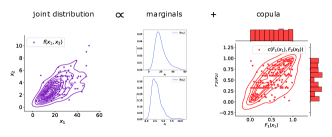
Figure 6: Expressing joint densities with copulas.

There exist many parametric representations through different copula families, however, to leverage even more flexibility, in this paper, we focus on the kernel-based nonparametric copulas of [60]. Eq. C.1 can be generalized and holds for any number of variables. To be able to fit densities of more than two variables, we make use of the pair copula constructions, namely vines; hierarchical models, constructed from cascades of bivariate copula blocks [61]. According to [62, 37], any $M$-dimensional copula density can be decomposed into a product of $\frac{M(M-1)}{2}$ bivariate (conditional) copula densities. Although such factorization may not be unique, it can be organized in a graphical model, as a sequence of $M-1$ nested trees, called vines. We denote a tree as $T_{m}=(V_{m},E_{m})$ with $V_{m}$ and $E_{m}$ the sets of nodes and edges of tree $m$ for $m=1,\dots,M-1$. Each edge $e$ is associated with a bivariate copula. An example of a vine copula decomposition is given in Fig. 7. In practice, in order to construct a vine, one chooses two components:

1. the structure, the set of trees $T_{m}=(V_{m},E_{m})$ for $m\in[M-1]$

2. the pair-copulas, the models for $c_{j_{e},k_{e}|D_{e}}$ for $e\in E_{m}$ and $m\in[M-1]$.

Corresponding algorithms exist for both of those steps and in the rest of the paper, we assume consistency of the vine copula estimators for which we use the implementation by [63].

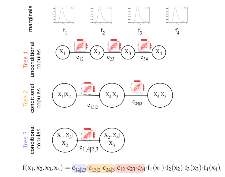
Figure 7: Multivariate joint density factorized with a vine copula.

Appendix D Experimental detail

We executed batched BO simulations with a batch size of $B=4$ for all the experiments. The number of iterations $T$ varied across the experiments. Other parameters include: the initial data size $N_{0}$, the size of the pool $N$, and the number of predictive posterior samples $L$. We fixed the size of the pool relative to the selected batch, at $N/B=100$. We also fixed $L=20$, which was found to yield good sample coverage and a stable BOtied acquisition value.

Unless otherwise stated, the surrogate model was a multi-task Gaussian process (MTGP) with a Matern kernel implemented in BoTorch [44] and GPyTorch [64]. The inputs and outputs were both scaled to the unit cube for fitting the MTGP, but the outputs were scaled back to their natural units for evaluating the respective acquisition functions.

D.1 Branin-Currin

Branin-Currin ($d=2$, $M=2$; [25]) is a composition of the Branin and Currin functions featuring a concave Pareto front (in the maximization setting). We maximize

$$f_{1}(x_{1},x_{2})=-\left(x_{2}-\frac{5.1}{4\pi^{2}}x_{1}^{2}+\frac{5}{\pi}x_{1}-r\right)^{2}+10(1-\frac{1}{8\pi})\cos(x_{1})+10$$

$$f_{2}(x_{1},x_{2})=-[1-\exp\left(-\frac{1}{2x_{2}}\right)]\frac{2300x_{1}^{3}+1900x_{1}^{2}+2092x_{1}+60}{100x_{1}^{3}+500x_{1}^{2}+4x_{1}+20},$$

where $x_{1},x_{2}\in[0,1]$. We used $T=30$.

D.2 DTLZ

For the DTLZ problem, we took DTLZ2 ($d=9$, $M\in\{4,6,8\}$; [46]) and used $T=20$.

D.3 Penicillin production

For the Penicillin production problem ($d=7$, $M=3$; [47]), we used $T=10$.

D.4 Caco2+

For the Caco2 problem ($M=3$; [48]), we use $T=10$. The objective is to identify molecules with maximum cell permeability. Here, permeability describes the degree to which a molecule passes through a cellular membrane. This property is critical for drug discovery (DD) programs where the disease protein being targeted resides within the cell (intracellularly). In each experiment, a molecule ${\bm{x}}_{i}$ is applied to a monolayer of Caco2 cells and, after incubation, the concentration $c$ of ${\bm{x}}_{i}$ is measured on both the input and output side of the monolayer, giving $c_{\rm in}$ and $c_{\rm out}$[65]. The ratio $c_{\rm out}/{c_{\rm in}}$ is then treated as the final permeability label $y^{p}_{i}$.

Cellular membranes are composed of a complex mixture of lipids and other biomolecules. In order to enter and (passively) diffuse through a membrane, molecule ${\bm{x}}_{i}$ should interact favorably with these biomolecules and/or avoid disrupting their packing structure. Increasing the lipophilicity (logP) of ${\bm{x}}_{i}$ is thus one strategy to increase permeability. However, increasing logP often results in promiscuous binding of ${\bm{x}}_{i}$ to non-disease related proteins, which can lead to undesired side-effects. As such, we seek to minimize the computed logP (clogP, $y^{l}_{i}$) in our optimization task and note that this could directly compete with (i.e., harm) permeability.

Lastly and related, common objectives during MPO in DD settings include increasing the affinity and specificity of target binding. As opposed to non-specific lipophilic interactions as above, polar contacts (such as hydrogen bonds) between drug molecules and proteins often result in higher affinity and more specific binding. We compute the topological polar surface area (TPSA, $y^{t}_{i}$) of each candidate $\textbf{x}_{i}$ as one indicator of its ability to form such interactions and seek to maximize it in our optimization. As with decreasing logP, increasing TPSA can negatively impact permeability and we thus consider it a competing objective.

It is important to note that the treatment of each of these optimization tasks as unidirectional (max or min) is a simplification of many practical DD settings. There is often an acceptable range of each value that is targeted, and leaving the bounds in either direction can be problematic for complex reasons. We direct the reader to [66] for a comprehensive review.

For fitting the MTGP on the Caco2+ data, we represent each input molecule as a concatenation of fingerprint and fragment feature vectors, known as fragprints [51] and use the Tanimoto kernel implemented in GAUCHE [67].

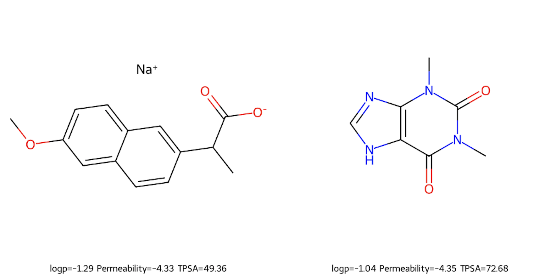
Figure 8: Examples of molecules with “good"/desirable TPSA, permeability, and ClogP values.

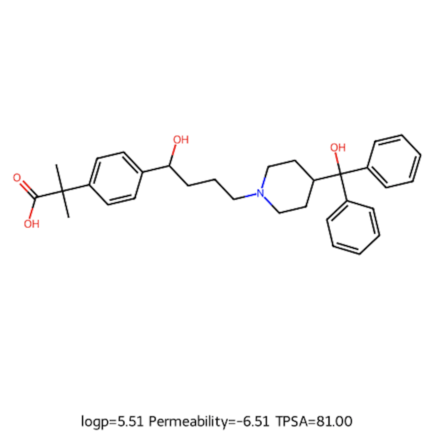
Figure 9: An example of a molecule with “bad" TPSA, permeability, and ClogP values.

References

- [1] Philip A Romero, Andreas Krause, and Frances H Arnold. Navigating the protein fitness landscape with gaussian processes. Proceedings of the National Academy of Sciences, 110(3):E193–E201, 2013.
- [2] Roberto Calandra, André Seyfarth, Jan Peters, and Marc Peter Deisenroth. Bayesian optimization for learning gaits under uncertainty: An experimental comparison on a dynamic bipedal walker. Annals of Mathematics and Artificial Intelligence, 76:5–23, 2016.
- [3] A Gilad Kusne, Heshan Yu, Changming Wu, Huairuo Zhang, Jason Hattrick-Simpers, Brian DeCost, Suchismita Sarker, Corey Oses, Cormac Toher, Stefano Curtarolo, et al. On-the-fly closed-loop materials discovery via bayesian active learning. Nature communications, 11(1):5966, 2020.
- [4] Benjamin J Shields, Jason Stevens, Jun Li, Marvin Parasram, Farhan Damani, Jesus I Martinez Alvarado, Jacob M Janey, Ryan P Adams, and Abigail G Doyle. Bayesian reaction optimization as a tool for chemical synthesis. Nature, 590(7844):89–96, 2021.
- [5] Yunxing Zuo, Mingde Qin, Chi Chen, Weike Ye, Xiangguo Li, Jian Luo, and Shyue Ping Ong. Accelerating materials discovery with bayesian optimization and graph deep learning. Materials Today, 51:126–135, 2021.
- [6] Hugo Bellamy, Abbi Abdel Rehim, Oghenejokpeme I Orhobor, and Ross King. Batched bayesian optimization for drug design in noisy environments. Journal of Chemical Information and Modeling, 62(17):3970–3981, 2022.
- [7] Asif Khan, Alexander I Cowen-Rivers, Antoine Grosnit, Philippe A Robert, Victor Greiff, Eva Smorodina, Puneet Rawat, Rahmad Akbar, Kamil Dreczkowski, Rasul Tutunov, et al. Toward real-world automated antibody design with combinatorial bayesian optimization. Cell Reports Methods, page 100374, 2023.
- [8] Ji Won Park, Samuel Stanton, Saeed Saremi, Andrew Watkins, Henri Dwyer, Vladimir Gligorijevic, Richard Bonneau, Stephen Ra, and Kyunghyun Cho. Propertydag: Multi-objective bayesian optimization of partially ordered, mixed-variable properties for biological sequence design. NeurIPS AI for Science workshop, 2022.
- [9] R Timothy Marler and Jasbir S Arora. Survey of multi-objective optimization methods for engineering. Structural and multidisciplinary optimization, 26:369–395, 2004.
- [10] Tushar Jain, Tingwan Sun, Stéphanie Durand, Amy Hall, Nga Rewa Houston, Juergen H Nett, Beth Sharkey, Beata Bobrowicz, Isabelle Caffry, Yao Yu, et al. Biophysical properties of the clinical-stage antibody landscape. Proceedings of the National Academy of Sciences, 114(5):944–949, 2017.
- [11] Nataša Tagasovska, Nathan C Frey, Andreas Loukas, Isidro Hötzel, Julien Lafrance-Vanasse, Ryan Lewis Kelly, Yan Wu, Arvind Rajpal, Richard Bonneau, Kyunghyun Cho, et al. A pareto-optimal compositional energy-based model for sampling and optimization of protein sequences. NeurIPS AI for Science workshop, 2022.
- [12] Joshua Knowles. Parego: A hybrid algorithm with on-line landscape approximation for expensive multiobjective optimization problems. IEEE Transactions on Evolutionary Computation, 10(1):50–66, 2006.
- [13] Biswajit Paria, Kirthevasan Kandasamy, and Barnabás Póczos. A flexible framework for multi-objective bayesian optimization using random scalarizations. In UAI, pages 766–776. PMLR, 2020.
- [14] Michael Emmerich. Single-and multi-objective evolutionary design optimization assisted by gaussian random field metamodels. PhD thesis, Dortmund, Univ., Diss., 2005, 2005.
- [15] Michael TM Emmerich, André H Deutz, and Jan Willem Klinkenberg. Hypervolume-based expected improvement: Monotonicity properties and exact computation. In 2011 IEEE Congress of Evolutionary Computation (CEC), pages 2147–2154. IEEE, 2011.
- [16] Samuel Daulton, Maximilian Balandat, and Eytan Bakshy. Differentiable expected hypervolume improvement for parallel multi-objective bayesian optimization. NeurIPS, 33:9851–9864, 2020.
- [17] Samuel Daulton, Maximilian Balandat, and Eytan Bakshy. Parallel bayesian optimization of multiple noisy objectives with expected hypervolume improvement. NeurIPS, 34:2187–2200, 2021.
- [18] André Deutz, Michael Emmerich, and Kaifeng Yang. The expected r2-indicator improvement for multi-objective bayesian optimization. In Evolutionary Multi-Criterion Optimization: 10th International Conference, EMO 2019, East Lansing, MI, USA, March 10-13, 2019, Proceedings 10, pages 359–370. Springer, 2019.
- [19] André Deutz, Kaifeng Yang, and Michael Emmerich. The r2 indicator: A study of its expected improvement in case of two objectives. In AIP Conference Proceedings, volume 2070, page 020054. AIP Publishing LLC, 2019.
- [20] Kaifeng Yang, Michael Emmerich, André Deutz, and Thomas Bäck. Efficient computation of expected hypervolume improvement using box decomposition algorithms. Journal of Global Optimization, 75:3–34, 2019.
- [21] Kerstin Dächert, Kathrin Klamroth, Renaud Lacour, and Daniel Vanderpooten. Efficient computation of the search region in multi-objective optimization. European Journal of Operational Research, 260(3):841–855, 2017.
- [22] José Miguel Hernández-Lobato, Matthew W Hoffman, and Zoubin Ghahramani. Predictive entropy search for efficient global optimization of black-box functions. NeurIPS, 27, 2014.
- [23] José Miguel Hernández-Lobato, Michael A Gelbart, Ryan P Adams, Matthew W Hoffman, and Zoubin Ghahramani. A general framework for constrained bayesian optimization using information-based search. 2016.
- [24] Amar Shah and Zoubin Ghahramani. Parallel predictive entropy search for batch global optimization of expensive objective functions. NeurIPS, 28, 2015.
- [25] Syrine Belakaria, Aryan Deshwal, and Janardhan Rao Doppa. Max-value entropy search for multi-objective bayesian optimization. NeurIPS, 32, 2019.
- [26] Matthew W Hoffman and Zoubin Ghahramani. Output-space predictive entropy search for flexible global optimization. In NeurIPS workshop on Bayesian Optimization, pages 1–5, 2015.
- [27] Ben Tu, Axel Gandy, Nikolas Kantas, and Behrang Shafei. Joint entropy search for multi-objective bayesian optimization. arXiv preprint arXiv:2210.02905, 2022.
- [28] Bobak Shahriari, Kevin Swersky, Ziyu Wang, Ryan P Adams, and Nando De Freitas. Taking the human out of the loop: A review of bayesian optimization. Proceedings of the IEEE, 104(1):148–175, 2015.
- [29] Peter I Frazier. A tutorial on bayesian optimization. arXiv preprint arXiv:1807.02811, 2018.
- [30] Jonas Močkus. On bayesian methods for seeking the extremum. In Optimization techniques IFIP technical conference, pages 400–404. Springer, 1975.
- [31] Donald R Jones, Matthias Schonlau, and William J Welch. Efficient global optimization of expensive black-box functions. Journal of Global optimization, 13(4):455–492, 1998.
- [32] Eckart Zitzler, Lothar Thiele, Marco Laumanns, Carlos M Fonseca, and Viviane Grunert Da Fonseca. Performance assessment of multiobjective optimizers: An analysis and review. IEEE Transactions on evolutionary computation, 7(2):117–132, 2003.
- [33] Carlos M Fonseca, Joshua D Knowles, Lothar Thiele, Eckart Zitzler, et al. A tutorial on the performance assessment of stochastic multiobjective optimizers. In Third international conference on evolutionary multi-criterion optimization (EMO 2005), volume 216, page 240, 2005.
- [34] Eckart Zitzler, Dimo Brockhoff, and Lothar Thiele. The hypervolume indicator revisited: On the design of pareto-compliant indicators via weighted integration. In Evolutionary Multi-Criterion Optimization: 4th International Conference, EMO 2007, Matsushima, Japan, March 5-8, 2007. Proceedings 4, pages 862–876. Springer, 2007.
- [35] Mark Fleischer. The measure of pareto optima applications to multi-objective metaheuristics. In Evolutionary Multi-Criterion Optimization: Second International Conference, EMO 2003, Faro, Portugal, April 8–11, 2003. Proceedings 2, pages 519–533. Springer, 2003.
- [36] Roger B Nelsen. An introduction to copulas. Springer Science & Business Media, 2007.
- [37] Tim Bedford and Roger M. Cooke. Vines – A New Graphical Model for Dependent Random Variables. The Annals of Statistics, 30(4):1031–1068, 2002.
- [38] A. Sklar. Fonctions de Répartition à n Dimensions et Leurs Marges. Publications de L’Institut de Statistique de L’Université de Paris, 8:229–231, 1959.
- [39] M Haugh. An introduction to copulas. quantitative risk management, 2016.
- [40] Tim Bedford and Roger M Cooke. Vines–a new graphical model for dependent random variables. The Annals of Statistics, 30(4):1031–1068, 2002.
- [41] Kjersti Aas. Pair-copula constructions for financial applications: A review. Econometrics, 4(4):43, October 2016.
- [42] Carlos M Fonseca, Luís Paquete, and Manuel López-Ibánez. An improved dimension-sweep algorithm for the hypervolume indicator. In 2006 IEEE international conference on evolutionary computation, pages 1157–1163. IEEE, 2006.
- [43] Hisao Ishibuchi, Naoya Akedo, and Yusuke Nojima. A many-objective test problem for visually examining diversity maintenance behavior in a decision space. In Proceedings of the 13th annual conference on Genetic and evolutionary computation, pages 649–656, 2011.
- [44] Maximilian Balandat, Brian Karrer, Daniel R. Jiang, Samuel Daulton, Benjamin Letham, Andrew Gordon Wilson, and Eytan Bakshy. BoTorch: A Framework for Efficient Monte-Carlo Bayesian Optimization. In NeurIPS, 2020.
- [45] Samuel Daulton, Sait Cakmak, Maximilian Balandat, Michael A Osborne, Enlu Zhou, and Eytan Bakshy. Robust multi-objective bayesian optimization under input noise. arXiv preprint arXiv:2202.07549, 2022.
- [46] Kalyanmoy Deb and Himanshu Gupta. Searching for robust pareto-optimal solutions in multi-objective optimization. In Evolutionary Multi-Criterion Optimization: Third International Conference, EMO 2005, Guanajuato, Mexico, March 9-11, 2005. Proceedings 3, pages 150–164. Springer, 2005.
- [47] Qiaohao Liang and Lipeng Lai. Scalable bayesian optimization accelerates process optimization of penicillin production. In NeurIPS 2021 AI for Science Workshop, 2021.
- [48] Ning-Ning Wang, Jie Dong, Yin-Hua Deng, Min-Feng Zhu, Ming Wen, Zhi-Jiang Yao, Ai-Ping Lu, Jian-Bing Wang, and Dong-Sheng Cao. Adme properties evaluation in drug discovery: prediction of caco-2 cell permeability using a combination of nsga-ii and boosting. Journal of Chemical Information and Modeling, 56(4):763–773, 2016.
- [49] Kexin Huang, Tianfan Fu, Wenhao Gao, Yue Zhao, Yusuf Roohani, Jure Leskovec, Connor W Coley, Cao Xiao, Jimeng Sun, and Marinka Zitnik. Therapeutics data commons: Machine learning datasets and tasks for drug discovery and development. NeurIPS Datasets and Benchmarks, 2021.
- [50] Kexin Huang, Tianfan Fu, Wenhao Gao, Yue Zhao, Yusuf Roohani, Jure Leskovec, Connor W Coley, Cao Xiao, Jimeng Sun, and Marinka Zitnik. Artificial intelligence foundation for therapeutic science. Nature Chemical Biology, 2022.
- [51] Aditya R Thawani, Ryan-Rhys Griffiths, Arian Jamasb, Anthony Bourached, Penelope Jones, William McCorkindale, Alexander A Aldrick, and Alpha A Lee. The photoswitch dataset: A molecular machine learning benchmark for the advancement of synthetic chemistry. arXiv preprint arXiv:2008.03226, 2020.
- [52] Greg Landrum, Paolo Tosco, Brian Kelley, Ric, sriniker, David Cosgrove, gedeck, Riccardo Vianello, NadineSchneider, Eisuke Kawashima, Dan N, Gareth Jones, Andrew Dalke, Brian Cole, Matt Swain, Samo Turk, AlexanderSavelyev, Alain Vaucher, Maciej Wójcikowski, Ichiru Take, Daniel Probst, Kazuya Ujihara, Vincent F. Scalfani, guillaume godin, Axel Pahl, Francois Berenger, JLVarjo, Rachel Walker, jasondbiggs, and strets123. rdkit/rdkit: 2023_03_1 (q1 2023) release, April 2023.
- [53] G Richard Bickerton, Gaia V Paolini, Jérémy Besnard, Sorel Muresan, and Andrew L Hopkins. Quantifying the chemical beauty of drugs. Nature chemistry, 4(2):90–98, 2012.
- [54] Scott A Wildman and Gordon M Crippen. Prediction of physicochemical parameters by atomic contributions. Journal of chemical information and computer sciences, 39(5):868–873, 1999.
- [55] Duxin Sun, Wei Gao, Hongxiang Hu, and Simon Zhou. Why 90% of clinical drug development fails and how to improve it? Acta Pharmaceutica Sinica B, 2022.
- [56] Mickaël Binois, Didier Rullière, and Olivier Roustant. On the estimation of pareto fronts from the point of view of copula theory. Information Sciences, 324:270–285, 2015.
- [57] Natasa Tagasovska, Firat Ozdemir, and Axel Brando. Retrospective uncertainties for deep models using vine copulas. In International Conference on Artificial Intelligence and Statistics, pages 7528–7539. PMLR, 2023.
- [58] Kjersti Aas, Claudia Czado, Arnoldo Frigessi, and Henrik Bakken. Pair-copula constructions of multiple dependence. Insurance: Mathematics and economics, 44(2):182–198, 2009.
- [59] Harry Joe, Haijun Li, and Aristidis K. Nikoloulopoulos. Tail dependence functions and vine copulas. Journal of Multivariate Analysis, 101(1):252–270, January 2010.
- [60] Gery Geenens, Arthur Charpentier, and Davy Paindaveine. Probit transformation for nonparametric kernel estimation of the copula density. Bernoulli, 23(3):1848–1873, 2017.
- [61] Thomas Nagler, Christian Schellhase, and Claudia Czado. Nonparametric estimation of simplified vine copula models: comparison of methods. Dependence Modeling, 5(1):99–120, 2017.
- [62] Harry Joe. Multivariate Models and Dependence Concepts. Chapman & Hall/CRC, 1997.
- [63] Thomas Nagler and Claudia Czado. Evading the curse of dimensionality in nonparametric density estimation with simplified vine copulas. Journal of Multivariate Analysis, 151:69–89, 2016.
- [64] Jacob R Gardner, Matt J Kusner, Zhixiang Eddie Xu, Kilian Q Weinberger, and John P Cunningham. Bayesian optimization with inequality constraints. In ICML, volume 2014, pages 937–945, 2014.
- [65] Richard B Van Breemen and Yongmei Li. Caco-2 cell permeability assays to measure drug absorption. Expert opinion on drug metabolism & toxicology, 1(2):175–185, 2005.
- [66] Matthew D. Segall. Multi-parameter optimization: identifying high quality compounds with a balance of properties. Current pharmaceutical design, 18(9):1292, 2012.
- [67] Ryan-Rhys Griffiths, Leo Klarner, Henry B. Moss, Aditya Ravuri, Sang Truong, Bojana Rankovic, Yuanqi Du, Arian Jamasb, Julius Schwartz, Austin Tripp, Gregory Kell, Anthony Bourached, Alex Chan, Jacob Moss, Chengzhi Guo, Alpha A. Lee, Philippe Schwaller, and Jian Tang. Gauche: A library for gaussian processes in chemistry, 2022.