Construction of inclusions with vanishing generalized polarization tensors by imperfect interfaces

Abstract

We investigate the problem of planar conductivity inclusion with imperfect interface conditions. We assume that the inclusion is simply connected. The presence of the inclusion causes a perturbation in the incident background field. This perturbation admits a multipole expansion of which coefficients we call the generalized polarization tensors (GPTs), extending the previous terminology for inclusions with perfect interfaces. We derive explicit matrix expressions for the GPTs in terms of the incident field, material parameters, and geometry of the inclusion. As an application, we construct GPT-vanishing structures of general shape that result in negligible perturbations for all uniform incident fields. The structure consists of a simply connected core with an imperfect interface. We provide numerical examples of GPT-vanishing structures obtained by our proposed scheme.

Mathematics Subject Classification. 35J05; 74B05; 65B99

Keywords. Geometric Multipole Expansion; Grunsky Coefficient; Imperfect Interface; GPT-vanishing structure

1 Introduction

We consider the planar conductivity (or anti-plane elasticity) problem, where an inclusion is inserted into an infinite homogeneous background. The inclusion, having a different conductivity from that of the background, generally induces perturbations to the background fields. However, certain types of inclusions do not cause any perturbation to the uniform background fields, known as neutral inclusions. Neutral inclusions have been extensively studied due to their possible applications in designing invisibility cloaking structures with metamaterials in various contexts, including acoustics, elasticity, electromagnetics, and microwaves [1, 5, 30, 32, 44, 45, 46]. Most results on neutral inclusions deal with perfect boundary conditions. On the other hand, this paper addresses neutral inclusions with imperfect interfaces. More precisely, we provide a construction scheme for neutral inclusions of general shape with imperfect interfaces conditions where the core has finite low conductivity.

Well-known examples of neutral inclusions (with perfect interfaces) that do not disturb incident uniform fields are coated disks and spheres with isotropic material parameters [18, 19, 20, 23, 35, 36]. Coated ellipses and ellipsoids exhibit neutrality to uniform fields of all directions when the conductivities of the core, shell, and matrix are appropriately selected (potentially anisotropic) [16, 29, 33, 40, 39]. It is worth noting that these are the only shapes that can achieve the neutral property for all uniform fields [25, 26, 34]. Non-elliptical coated inclusions can achieve neutrality for a single uniform field [21, 34] (see also [31]).

One can design neutral inclusions using the concept of the generalized polarization tensors (GPTs), which are the coefficients of the multipole expansion for the perturbed potential caused by the inclusion; this concept extends the polarization tensor, introduced by Schiffer and Szegö [38], to higher orders. GPT-vanishing structures–inclusions with vanishing values for the leading-order terms of the GPTs–are neutral inclusions in the asymptotic sense. Multi-coated concentric disks or balls have been reported to be GPT-vanishing structures [4, 43] (see also [3, 5] for results in the context of Helmholtz and Maxwell’s equations). GPT-vanishing structures of general shape were also obtained using a shape optimization approach [15, 22, 28] (see also [11]).

Imperfect interfaces are characterized by discontinuity in either the flux or the potential, in contrast to perfectly bonding boundaries of which both the flux and potential are continuous. The interface parameter, possibly a non-constant function, accounts for the discontinuity of the flux or the potential on the interface. In [37], Ru investigated neutral inclusions for the two-dimensional elastic problem with imperfect interfaces when the inclusion is stiffer than the background medium. For the conductivity problem, Benveniste and Miloh found neutral inclusions with imperfect interfaces for a single uniform field [8]. In [27], Kang and Li constructed PT-vanishing structures of general shape with imperfect interfaces, assuming that the core is simply connected and perfectly conducting.

In this paper, we propose a new construction scheme of neutral inclusions (of general shape) for the planar conductivity problem with imperfect interfaces. The inclusions have discontinuity in the potential, where the core have the arbitrary constant conductivity. Different from [27], the constant potential condition in the core is no longer assumed. Consequently, the construction of the interface parameter satisfying the neutrality condition becomes challenging. To address this problem, we find GPT-vanishing structures by employing the concept of the Faber polynomials polarization tensors (FPTs) (see [11]). The FPTs are linear combinations of GPTs with coefficients given by Faber polynomials associated with the inclusion. We also refer to [13, 14] for details of Faber polynomials. The concept of FPTs has been successfully applied to design semi-neutral inclusions [11] (see also [9, 10, 24]). In this paper, we derive an explicit matrix expression of the FPTs for an inclusion with imperfect interface conditions and, by using the matrix expression, determine the interface parameter that vanishes several leading terms of the FPTs.

The rest of this paper is organized as follows. In Section 2, we present the problem formulation. In Section 3, we introduce Faber polynomials based on conformal mappings and define the FPTs using integral formulation. Section 4 focuses on deriving the matrix expressions for the FPTs. The construction scheme for inclusions with vanishing GPTs (or FPTs) by imperfect interfaces is described in Section 5. We also present numerical visualizations in Section 5.

2 Problem formulation

We let $D$ be a planar, simply connected domain with an analytic boundary. The core region $D$ has the constant conductivity $\sigma_{c}$ and the exterior region $\mathbb{R}^{2}\setminus D$ is occupied by another homogeneous isotropic material with the constant conductivity $\sigma_{m}>0$. We consider the potential problem with imperfect interface condition:

$$\begin{cases}\displaystyle\nabla\cdot{\sigma}\nabla u=0\qquad&\mbox{in }\mathbb{\mathbb{R}}^{2},\\ \displaystyle p\big{(}u\big{|}^{+}-u\big{|}^{-}\big{)}=\sigma_{m}\frac{\partial u}{\partial\nu}\Big{|}^{+}\qquad&\mbox{on }\partial D,\\[5.69054pt] \displaystyle\sigma_{m}\frac{\partial u}{\partial\nu}\Big{|}^{+}=\sigma_{c}\frac{\partial u}{\partial\nu}\Big{|}^{-}\qquad&\mbox{on }\partial D,\\[5.69054pt] \displaystyle(u-H)(x)=O({|x|^{-1}})\qquad&\mbox{as }|x|\to\infty,\end{cases}$$ (2.1)

where $p$ is the interface parameter that is a real-valued function on $\partial\Omega$ and $H$ is an arbitrary entire harmonic function. The conductivity distribution ${\sigma}$ has the form

$${\sigma}=\sigma_{c}\chi_{D}+\sigma_{m}\chi_{\mathbb{R}^{2}\setminus\overline{D}},$$

where $\chi$ is the characteristic function.

2.1 Generalized polarization tensors

For a Lipschitz domain $D$, we define the single and double layer potentials with a density $\varphi\in L^{2}(\partial D)$,

$$\mathcal{S}_{\partial D}[\varphi](x) =\int_{\partial D}\Gamma(x-y)\varphi(y)\,d\sigma(y),\quad x\in\mathbb{R}^{2},$$

$$\mathcal{D}_{\partial D}[\varphi](x) =\int_{\partial D}\frac{\partial}{\partial\nu_{y}}\Gamma(x-y)\varphi(y)\,d\sigma(y),\quad x\in\mathbb{R}^{2}\setminus\partial D,$$

where $\Gamma$ is the fundamental solution to the Laplacian, i.e., $\Gamma(x)=\frac{1}{2\pi}\ln|x|$, and $\nu_{y}$ denotes the outward unit normal vector on $\partial D$. We also define the so-called Neumann–Poincaré (NP) operator

$$\mathcal{K}_{\partial D}[\varphi](x)=p.v.\,\int_{\partial D}\frac{\partial}{\partial\nu_{y}}\Gamma(x-y)\varphi(y)\,d\sigma(y),\quad x\in\partial D,$$

and its $L^{2}$-adjoint operator

$$\mathcal{K}^{*}_{\partial D}[\varphi](x)=p.v.\,\int_{\partial D}\frac{\partial}{\partial\nu_{x}}\Gamma(x-y)\varphi(y)\,d\sigma(y),\quad x\in\partial D.$$

Here, $p.v.$ stands for the Cauchy principal value. The operator $\mathcal{K}^{*}_{\partial D}$ is bounded on $L^{2}(\partial D)$. We identify $x=(x_{1},x_{2})\in\mathbb{R}^{2}$ with $z=x_{1}+\mathrm{i}x_{2}\in\mathbb{C}$. We set

$$\mathcal{S}_{\partial D}[\varphi](z):=\mathcal{S}_{\partial D}[\varphi](x).$$

Likewise, we define $\mathcal{D}_{\partial D}[\varphi](z)$ and $\mathcal{K}^{*}_{\partial D}[\varphi](z)$.

On the interface $\partial D$, the layer potentials satisfy the jump relations

$$\mathcal{S}_{\partial D}[\varphi]\Big{|}^{+} =\mathcal{S}_{\partial D}[\varphi]\Big{|}^{-},$$

$$\frac{\partial}{\partial\nu}\mathcal{S}_{\partial D}[\varphi]\Big{|}^{\pm} =\left(\pm\frac{1}{2}I+\mathcal{K}^{*}_{\partial D}\right)[\varphi],$$

$$\mathcal{D}_{\partial D}[\varphi]\Big{|}^{\pm} =\left(\mp\frac{1}{2}I+\mathcal{K}_{\partial D}\right)[\varphi],$$

$$\frac{\partial}{\partial\nu}\mathcal{D}_{\partial D}[\varphi]\Big{|}^{+} =\frac{\partial}{\partial\nu}\mathcal{D}_{\partial D}[\varphi]\Big{|}^{-}.$$

Here, $I$ denotes the identity operator on $L^{2}(\partial D)$.

Let $\Re[\cdot]$ and $\Im[\cdot]$ denote the real and imaginary part of a complex number, respectively. The solution $u$ of the system (2.1) can be represented by

$$u(z)=H(z)+\left(\mathcal{S}_{\partial D}\,p-\tau\mathcal{D}_{\partial D}\right)[\varphi](z),\quad(\Re(z),\Im(z))\in\mathbb{R}^{2}\setminus{\partial D}$$ (2.2)

with $\lambda=\frac{\sigma_{c}+\sigma_{m}}{2(\sigma_{c}-\sigma_{m})}$ and $\tau=\frac{\sigma_{c}\sigma_{m}}{\sigma_{c}-\sigma_{m}},$ where $p$ denotes the multiplication operator by $p$ (by abuse of the notation) and the density function $\varphi$ is the solution to the integral equation

$$\left(\left(\lambda I-\mathcal{K}^{*}_{\partial D}\right)p+\tau\frac{\partial}{\partial\nu}\mathcal{D}_{\partial D}\right)\left[\varphi\right]=\frac{\partial H}{\partial\nu}.$$ (2.3)

This representation was introduced in [27] for the case $\sigma_{c}=\infty$ (that is, $\tau=1$) with arbitrary smooth function $p>0$. Following the proof in [27], one can show that the operator $\left(\lambda I-\mathcal{K}^{*}_{\partial D}\right)p+\tau\frac{\partial}{\partial\nu}\mathcal{D}_{\partial D}$ is invertible for $0<\sigma\neq 1<\infty$. By the jump relations, the solution (2.2) meets all conditions of the system (2.1).

Definition 1.

Set $Z_{n}(\eta)=\eta^{n}$ for each $n\in\mathbb{N}$. For $m,n\in\mathbb{N}$, we define

$$\mathbb{N}_{mn}^{(1)}(D,p,\sigma_{c},\sigma_{m}) =\int_{\partial D}\bigg{(}Z_{n}(\eta)\,p(\eta)-\tau\frac{\partial Z_{n}(\eta)}{\partial\nu}\bigg{)}\bigg{(}(\lambda I-\mathcal{K}^{*}_{\partial D})p+\tau\frac{\partial\mathcal{D}_{\partial D}}{\partial\nu}\bigg{)}^{-1}\left[\frac{\partial Z_{m}}{\partial\nu}\right](\eta)\,d\sigma(\eta),$$

$$\mathbb{N}_{mn}^{(2)}(D,p,\sigma_{c},\sigma_{m}) =\int_{\partial D}\bigg{(}Z_{n}(\eta)\,p(\eta)-\tau\frac{\partial Z_{n}(\eta)}{\partial\nu}\bigg{)}\bigg{(}(\lambda I-\mathcal{K}^{*}_{\partial D})p+\tau\frac{\partial\mathcal{D}_{\partial D}}{\partial\nu}\bigg{)}^{-1}\left[\frac{\partial\overline{Z_{m}}}{\partial\nu}\right](\eta)\,d\sigma(\eta),$$

where $\lambda=\frac{\sigma_{c}+\sigma_{m}}{2(\sigma_{c}-\sigma_{m})}$ and $\tau=\frac{\sigma_{c}\sigma_{m}}{\sigma_{c}-\sigma_{m}}$. We call $\mathbb{N}_{mn}^{(1)}$ and $\mathbb{N}_{mn}^{(2)}$ the (complex) generalized polarization tensors (GPTs) corresponding to the inclusion $D$ with the interface function $p$ and the conductivities $\sigma_{c}$, $\sigma_{m}$.

The GPTs generalize the polarization tensor (PT) that was introduced by Schiffer and Szegö [38]. The concept of the PT, the GPTs for $m=n=1$, is applicable to the potential problem with imperfect interface condition.

2.2 Multipole expansion

Using this Taylor expansion, the solution expression (2.2) and the definition of the GPTs, one can show the following multipole expansion for the inclusion problem with imperfect interface (refer to [2, 6, 7, 42] for the perfect interface problem).

Proposition 2.1.

Let $u$ be the solution to (2.1) for $H(z)=\Re\left[\sum_{m=1}^{\infty}\alpha_{m}z^{m}\right]$ with complex coefficients $\alpha_{m}$. Let $\mathbb{N}_{mn}^{(1)}$ and $\mathbb{N}_{mn}^{(2)}$ be given by Definition 1. We have

$$u(z)=H(z)-\Re\left[\sum_{n=1}^{\infty}\sum_{m=1}^{\infty}\frac{1}{4\pi n}\left(\alpha_{m}\mathbb{N}_{mn}^{(1)}+\overline{\alpha_{m}}\,\mathbb{N}_{mn}^{(2)}\right){z^{-n}}\right],\quad|z|>\sup\left\{|y|:y\in D\right\}.$$

Proof.

By the Taylor expansion of the logarithmic function, we get as $|z|\to\infty$,

$$\Gamma(z-\eta)=\frac{1}{2\pi}\Re\left[\ln(z-\eta)\right]=\frac{1}{2\pi}\Re\bigg{[}\ln z-\sum_{n=1}^{\infty}\frac{1}{n}\frac{\eta^{n}}{z^{n}}\bigg{]}=\Gamma(z)-\sum_{n=1}^{\infty}\frac{1}{2\pi n}\Re\left[Z_{n}(\eta)\,z^{-n}\right].$$

Using this expansion and (2.2), the solution $u$ satisfies

$$u(z) =H(z)+\mathcal{S}_{\partial D}[p\varphi](z)-\tau\mathcal{D}_{\partial D}[\varphi](z)$$

$$=H(z)+\int_{\partial D}\left[\Gamma(z-\eta)\,p(\eta)-\tau\frac{\partial\Gamma(z-\eta)}{\partial\nu_{\eta}}\right]\varphi(\eta)\,d\sigma(\eta)$$

$$=H(z)+\int_{\partial D}\Gamma(z)\,p(\eta)\,\varphi(\eta)\,d\sigma(\eta)$$

$$\quad-\sum_{n=1}^{\infty}\frac{z^{-n}}{2\pi n}\int_{\partial D}\Re\left[Z_{n}(\eta)\,p(\eta)-\tau\frac{\partial Z_{n}(\eta)}{\partial\nu_{\eta}}\right]\varphi(\eta)\,d\sigma(\eta)$$

$$=H(z)-\sum_{n=1}^{\infty}\frac{z^{-n}}{2\pi n}\int_{\partial D}\Re\left[Z_{n}(\eta)\,p(\eta)-\tau\frac{\partial Z_{n}(\eta)}{\partial\nu_{\eta}}\right]\varphi(\eta)\,d\sigma(\eta).$$ (2.4)

The last equation holds because $\int_{\partial D}p(\eta)\,\varphi(\eta)\,d\sigma(\eta)=0$. Due to (2.3), we have

$$\varphi=\left(\left(\lambda I-\mathcal{K}^{*}_{\partial D}\right)p+\tau\frac{\partial}{\partial\nu}\mathcal{D}_{\partial D}\right)^{-1}\left[\Re\left(\sum_{m=1}^{\infty}\alpha_{m}\frac{\partial Z_{m}}{\partial\nu}\right)\right],$$

and substituting this $\varphi$ into (2.4) leads the desired result. $\Box$

In [27], the interface function $p$ was constructed such that the corresponding PT, i.e., $\mathbb{N}_{11}^{(1)}$ and $\mathbb{N}_{11}^{(2)}$, vanishes under the assumption that $\sigma_{c}=\infty$ (that is, the core is occupied with perfectly conducting material).

In the present paper, we construct the interface function $p$ such that the GPTs vanish up to some finite orders (including the PT), where the core $D$ is a given domain with arbitrary constant conductivity $\sigma_{c}$. In view of Proposition 2.1, the resulting inclusion is a neutral inclusion in the asymptotic sense. For the construction of $p$, we will apply the complex potential approach in [11], where the concept of the Faber polynomial polarization tensors was employed to build semi-neutral inclusions of general shape.

3 Faber polynomial polarization tensors (FPTs)

From the Riemann mapping theorem, there uniquely exist $\gamma>0$ and conformal mapping $\Psi$ from $\{w\in\mathbb{C}:|w|>\gamma\}$ onto $\mathbb{C}\setminus\overline{D}$ such that

$$\Psi(w)=w+a_{0}+\frac{a_{1}}{w}+\frac{a_{2}}{w^{2}}+\cdots.$$ (3.1)

The quantity $\gamma$ is called the conformal radius of $D$. One can numerically compute the numerical computation of $a_{n}$ from a given parametrization of $\partial\Omega$ (see, for instance, [24]). As an univalent function, $\Psi$ defines the Faber polynomials $\{F_{m}\}_{m=1}^{\infty}$ by the relation [13]

$$\frac{\Psi^{\prime}(w)}{\Psi(w)-z}=\sum_{m=0}^{\infty}\frac{F_{m}(z)}{w^{m+1}},\quad z\in{\overline{D}},\ |w|>\gamma.$$ (3.2)

The Faber polynomials $F_{m}$ are monic polynomials of degree $m$ that are uniquely determined by the conformal mapping coefficients $\{a_{n}\}_{0\leq n\leq m-1}$ via the recursive relation [12]:

$$F_{m+1}(z)=zF_{m}(z)-ma_{m}-\sum_{n=0}^{m}a_{n}F_{m-n}(z),\quad m\geq 0.$$ (3.3)

In particular, we have

$$F_{0}(z) =1,\quad F_{1}(z)=z-a_{0},\quad F_{2}(z)=z^{2}-2a_{0}z+a_{0}^{2}-2a_{1},$$

$$F_{3}(z) =z^{3}-3a_{0}z^{2}+3(a_{0}^{2}-a_{1})z-a_{0}^{3}+3a_{0}a_{1}-3a_{2}.$$

For $z=\Psi(w)$ with $|w|>r$, it holds that

$$F_{m}(\Psi(w))=w^{m}+\sum_{n=1}^{\infty}c_{mn}{w^{-n}}$$ (3.4)

with the so-called Grunsky coefficient $c_{mn}$. Recursive relations for the Faber polynomial coefficients and the Grunsky coefficients are well-known (see, for instance, [12, 17]).

We introduce the modified polar coordinates $(\rho,\theta)\in[\rho_{0},\infty)\times[0,2\pi)$, $\rho_{0}=\ln\gamma$, for $z\in\mathbb{C}\setminus D$ via the relation

$$z=\Psi(w)=\Psi(e^{\rho+i\theta}).$$

We denote the scale factor as $h=\left|\frac{\partial\Psi}{\partial\rho}\right|=\left|\frac{\partial\Psi}{\partial\theta}\right|=e^{\rho}\left|\Psi^{\prime}\right|.$ One can easily see that $d\sigma(z)=h(\rho_{0},\theta)d\theta$ on $\partial D$. For $z=\Psi(w)\in\partial D$, we have

$$\frac{\partial u}{\partial\nu}\Big{|}_{\partial D}^{\pm}=\frac{1}{h(\rho_{0},\theta)}\frac{\partial}{\partial\rho}u(\Psi(w))\Big{|}_{\rho\rightarrow\rho_{0}^{\pm}}.$$ (3.5)

We assume that $\Omega$ has an analytic boundary, that is, $\Psi$ can be conformally extended to $\{w\in\mathbb{C}:|w|>\gamma-\delta\}$ for some $\delta>0$. Then (3.2) holds with a modified conformal radius and domain. The Grunsky coefficients satisfy the so-called strong and week Grunsky inequalities. In particular, it holds that $\left|c_{mn}\right|\leq 2m\gamma^{m+n}.$ The same relation holds with $\gamma-\delta$ instead of $\gamma$, that is,

$$\left|c_{mn}\right|\leq 2m(\gamma-\delta)^{m+n}.$$ (3.6)

The Faber polynomials form a basis for complex analytic functions in $D$ [12]. Let $v$ be a complex analytic function in $D$ and continuous in $\overline{D}$. By applying the Cauchy integral formula to $v$ and applying (3.2), it follows that

$$v(z)=\sum_{m=0}^{\infty}b_{m}F_{m}(z)\quad\mbox{in }D$$

with $b_{m}=\frac{1}{2\pi i}\int_{|w|=\gamma}\frac{v(\Psi(w))}{w^{m+1}}\,dw.$ Hence, we have

$$|b_{m}|\leq\|v\|_{L^{\infty}(\partial D)}\gamma^{-m}.$$ (3.7)

3.1 FPTs and FPTs-vanishing structure

Since the Faber polynomials form a basis for complex analytic functions, $H$ is given by

$$H(z)=\sum_{m=1}^{\infty}\Re\big{[}\alpha_{m}F_{m}(z)\big{]}$$ (3.8)

with some complex coefficients $\alpha_{m}$.

Let $u$ be the solution to the imperfect interface problem (2.1). We can expand $u\big{|}_{D}$ into the real parts of the Faber polynomials. Furthermore, as the solution to (2.1) linearly depends on the background solution $H$, we have

$$u(z) =\sum_{m=1}^{\infty}\Re\bigg{[}\sum_{n=1}^{\infty}\beta_{mn}F_{n}(z)\bigg{]}\quad\mbox{in }D$$ (3.9)

with some constants $\beta_{mn}$. As $u-H$ is decaying near infinity and $\Psi$ is conformal, it holds that for $z=\Psi(w)$,

$$u(z)=H(z)+\sum_{m=1}^{\infty}\Re\bigg{[}\sum_{n=1}^{\infty}s_{mn}w^{-n}\bigg{]}\quad\mbox{in }\mathbb{R}^{2}\setminus\overline{D}$$ (3.10)

with some constants $s_{mn}$. Following [11], we call the expansion in (3.10) the geometric multipole expansion of $u$. For each $m$, both $\beta_{mn}$ and $s_{mn}$ are determined by $\alpha_{m}$. In particular, $\beta_{mn}=s_{mn}=0$ if we give $\alpha_{m}=0$ for some $m$ in (3.8). In fact, we can decompose the coefficient $s_{mn}$ by using some quantities defined as below.

Definition 1.

Let $F_{n}$ be the Faber polynomial for each $n\in\mathbb{N}$. For $m,n\in\mathbb{N}$, we define

$$\mathbb{F}_{mn}^{(1)}(D,p,\sigma_{c},\sigma_{m}) =\int_{\partial D}\bigg{(}F_{n}(\eta)\,p(\eta)-\tau\frac{\partial F_{n}(\eta)}{\partial\nu}\bigg{)}\bigg{(}(\lambda I-\mathcal{K}^{*}_{\partial D})p+\tau\frac{\partial\mathcal{D}_{\partial D}}{\partial\nu}\bigg{)}^{-1}\left[\frac{\partial F_{m}}{\partial\nu}\right](\eta)\,d\sigma(\eta),$$

$$\mathbb{F}_{mn}^{(2)}(D,p,\sigma_{c},\sigma_{m}) =\int_{\partial D}\bigg{(}F_{n}(\eta)\,p(\eta)-\tau\frac{\partial F_{n}(\eta)}{\partial\nu}\bigg{)}\bigg{(}(\lambda I-\mathcal{K}^{*}_{\partial D})p+\tau\frac{\partial\mathcal{D}_{\partial D}}{\partial\nu}\bigg{)}^{-1}\left[\frac{\partial\overline{F_{m}}}{\partial\nu}\right](\eta)\,d\sigma(\eta),$$

where $\lambda=\frac{\sigma_{c}+\sigma_{m}}{2(\sigma_{c}-\sigma_{m})}$ and $\tau=\frac{\sigma_{c}\sigma_{m}}{\sigma_{c}-\sigma_{m}}$. We call $\mathbb{F}_{mn}^{(1)}$ and $\mathbb{F}_{mn}^{(2)}$ the Faber polynomial polarization tensors (FPTs) for an inclusion with an imperfect interface, by extending the definition for an inclusion with perfect interface conditions in [11].

For $z=\Psi(w)$, integrating the expansion (3.2) with respect to $w$ yields that

$$\frac{1}{2\pi}\ln(z-\eta)=-\sum_{m=0}^{\infty}\frac{F_{m}(\eta)}{2\pi m}\frac{1}{w^{m}}+\text{constant},\quad\eta\in{\overline{D}},\ |w|>\gamma.$$

By using the linear dependence of $u$ on $H$ and the above series expansion, we can decompose $s_{mn}$ as

$$s_{mn}=-\alpha_{m}\frac{\mathbb{F}_{mn}^{(1)}}{4\pi n}-\overline{\alpha_{m}}\,\frac{\mathbb{F}_{mn}^{(2)}}{4\pi n},$$ (3.11)

where $\mathbb{F}_{mn}^{(1)}$ and $\mathbb{F}_{mn}^{(2)}$ are the FPTs independent of $\alpha_{m}$, namely,

$$u(z)=H(z)-\sum_{m=1}^{\infty}\Re\bigg{[}\sum_{n=1}^{\infty}\frac{1}{4\pi n}\left(\alpha_{m}\mathbb{F}_{mn}^{(1)}+\overline{\alpha_{m}}\mathbb{F}_{mn}^{(2)}\right)w^{-n}\bigg{]}\quad\mbox{in }\mathbb{R}^{2}\setminus\overline{D},$$ (3.12)

where $H$ is given by an entire Faber series $H(z)=\sum_{m=1}^{\infty}\Re\big{[}\alpha_{m}F_{m}(z)\big{]}$. We omit the derivation of (3.12) because it is very similar with the proof of Proposition 2.1.

The first-order terms of the FPTs correspond to the PTs considered in [27]. More precisely, the polarization tensor $M=\{m_{ij}\}_{i,j=1,2}$ admits the expression

$$M=\left(\begin{array}[]{cc}m_{11}&m_{12}\\ m_{21}&m_{22}\end{array}\right)=\frac{1}{2}\left(\begin{array}[]{cc}\displaystyle\Re\left[\mathbb{F}_{11}^{(1)}+\mathbb{F}_{11}^{(2)}\right]&\displaystyle\Im\left[\mathbb{F}_{11}^{(1)}+\mathbb{F}_{11}^{(2)}\right]\\[5.69054pt] \displaystyle\Im\left[\mathbb{F}_{11}^{(1)}-\mathbb{F}_{11}^{(2)}\right]&\displaystyle\Re\left[\mathbb{F}_{11}^{(2)}-\mathbb{F}_{11}^{(1)}\right]\end{array}\right).$$

We can express the Faber polynomial $F_{m}(z)$ as

$$F_{m}(z)=\sum_{n=0}^{m}q_{mn}z^{n},$$ (3.13)

where for a fixed $m$, the coefficient $q_{mn}$ depends only on $\{a_{k}\}_{0\leq k\leq m-1}$. One can easily obtain recursive formulas for $q_{mn}$ from (3.3). From (3.13) and the definition of the FPTs, it holds for each $m,n$ that

$$\mathbb{F}_{mn}^{(1)} =\sum_{k=1}^{m}\sum_{l=1}^{n}q_{mk}\,q_{nl}\,\mathbb{N}_{kl}^{(1)},$$ (3.14)

$$\mathbb{F}_{mn}^{(2)} =\sum_{k=1}^{m}\sum_{l=1}^{n}\overline{q_{mk}}\,q_{nl}\,\mathbb{N}_{kl}^{(2)}.$$

From the relations of the GPTs and FPTs, we can then obtain matrix factorizations for the GPTs. Set $Q=(q_{mn})_{m,n=1}^{\infty}$ with $q_{mn}$ given by (3.13). We can rewrite relations (3.14) in matrix form as

$$\mathbb{F}^{(1)} =Q\,\mathbb{N}^{(1)}Q^{T},$$ (3.15)

$$\mathbb{F}^{(2)} =\overline{Q}\,\mathbb{N}^{(2)}Q^{T},$$

where $\overline{Q}$ and $Q^{T}$ denote the conjugate and transpose matrices of $Q$, respectively. Using the recursive relation in (3.3), we get that, for each $m\geq 1$,

$$q_{mm}=1,\quad q_{(m+1)m}=-(m+1)a_{0},\quad q_{mn}=0\quad\mbox{for all }n\geq m+1.$$ (3.16)

Indeed,

$$Q=\left[\begin{matrix}1&0&0\quad\cdots\\[4.2679pt] -2a_{0}&1&0\quad\cdots\\[4.2679pt] 3a_{0}^{2}-3a_{1}&-3a_{0}&1\quad\cdots\\[4.2679pt] \vdots&\vdots&\vdots\quad\ddots\end{matrix}\right],$$ (3.17)

and then $Q$ is lower triangular and invertible. Consequently, (3.15) gives that

$$\mathbb{N}^{(1)} =Q^{-1}\,\mathbb{F}^{(1)}\left(Q^{-1}\right)^{T},$$ (3.18)

$$\mathbb{N}^{(2)} =\overline{Q^{-1}}\,\mathbb{F}^{(2)}\left(Q^{-1}\right)^{T}.$$

Indeed, the first terms of CGPTs and FPTs are always identical:

$$\mathbb{N}_{11}^{(1)}=\mathbb{F}_{11}^{(1)},\quad\mathbb{N}_{11}^{(2)}=\mathbb{F}_{11}^{(2)}.$$

Furthermore, if the center of the conformal mapping in (3.1) is given by $0$, namely, $a_{0}=0$, the lower diagonal elements $Q$ in (3.17) are all zero. In this case, CGPTs and FPTs have the same leading terms of order up to 2:

$$\mathbb{N}_{mn}^{(1)}=\mathbb{F}_{mn}^{(1)},\quad\mathbb{N}_{mn}^{(2)}=\mathbb{F}_{mn}^{(2)},\quad 1\leq m,n\leq 2.$$

Recall that our aim is to construct $p$ such that the corresponding GPTs vanish up to some finite orders. In view of (3.14) the GPT-vanishing structures can be equivalently achieved by the FPT-vanishing structure. It is worth remarking that for the instance of the perfectly bonding interface, explicit formulas of the FPTs were derived in [11].

4 Matrix expressions for the FPTs

Let $H$ be an entire harmonic function given by (3.8) and $u$ be the solution to (2.1). From (3.9), (3.9), (3.8) and the fact that $\Psi$ admits an analytic extension for $\rho\in[\rho_{0}-\delta,\rho_{0}]$, we have for $z=\Psi(w)$ that

$$u(z) =\begin{cases}\displaystyle\Re\bigg{[}\sum_{m=1}^{\infty}\sum_{n=1}^{\infty}\beta_{mn}F_{n}(z)\bigg{]}\quad&\mbox{for }\rho\in[\rho_{0}-\delta,\rho_{0}],\\ \displaystyle\Re\bigg{[}\sum_{m=1}^{\infty}\alpha_{m}F_{m}(z)+\sum_{m=1}^{\infty}\sum_{n=1}^{\infty}s_{mn}w^{-n}\bigg{]}\quad&\mbox{for }\rho>\rho_{0}\end{cases}$$

$$=\begin{cases}\displaystyle\Re\bigg{[}\sum_{m=1}^{\infty}\sum_{n=1}^{\infty}\beta_{mn}w^{n}+\sum_{m=1}^{\infty}\sum_{n=1}^{\infty}\sum_{l=1}^{\infty}\beta_{ml}c_{ln}w^{-n}\bigg{]}\quad&\mbox{for }\rho\in[\rho_{0}-\delta,\rho_{0}],\\ \displaystyle\Re\bigg{[}\sum_{m=1}^{\infty}\alpha_{m}w^{m}+\sum_{m=1}^{\infty}\sum_{n=1}^{\infty}\left(\alpha_{m}c_{mn}+s_{mn}\right)w^{-n}\bigg{]}\quad&\mbox{for }\rho>\rho_{0}\end{cases}$$ (4.1)

Since we only consider the background solution $H$ of finite order, we can assume finite summation for $m$. We may assume a finite summation for $m$ since only finite order polynomials are considered for $H$. For decaying properties of $\beta_{mn}$ and $c_{ln}$, we refer to (3.6) and (3.7).

The following lemma is useful to derive equivalent coefficients relations for a complex series to satisfy a boundary condition.

Lemma 4.1.

Let $\sum_{n=-\infty}^{\infty}c_{n}w^{n}$ be a complex analytic function in a neighborhood of $\{|w|=\gamma\}$. Then $\Re\left[\sum_{n=-\infty}^{\infty}c_{n}w^{n}\right]=0$ on $|w|=\gamma$ if and only if $c_{-n}+\overline{c_{n}}\gamma^{2n}=0$ for each $n\geq 0$.

Proof.

Since $\overline{w}=\gamma^{2}w^{-1}$ on $|w|=\gamma$, we have $2\Re\left[\sum_{n=-\infty}^{\infty}c_{n}w^{n}\right]=\sum_{n=-\infty}^{\infty}\left(c_{n}w^{n}+\overline{c_{n}w^{n}}\right)=\sum_{n=-\infty}^{\infty}\left(c_{-n}+\overline{c_{n}}\gamma^{2n}\right)w^{-n}.$ This proves the lemma. $\Box$

4.1 Equivalent relations for the boundary conditions

Let us define semi-infinite matrices

$$\boldsymbol{\alpha} =\big{\{}\alpha_{m}\delta_{mn}\big{\}}_{m,n\geq 1},\quad\boldsymbol{\beta}=\big{\{}\beta_{mn}\big{\}}_{m,n\geq 1},\quad\boldsymbol{s}=\big{\{}s_{mn}\big{\}}_{m,n\geq 1},$$ (4.2)

$$\mathcal{N} =\big{[}n\delta_{mn}\big{]}_{m,n\geq 1},\quad\gamma^{\tau\mathcal{N}}=\big{\{}\gamma^{\tau n}\delta_{mn}\big{\}}_{m,n\geq 1},\quad C=\big{\{}c_{mn}\big{\}}_{m,n\geq 1},$$

where $\delta_{mn}$ is the Kronecker-Delta function and $\tau\in\mathbb{R}$.

Lemma 4.1.

For $u$ given by (4.1), the condition $\frac{\partial u}{\partial\nu}\left|{}^{+}=\sigma_{c}\frac{\partial u}{\partial\nu}\right|^{-}$ is equivalent to the relation between the coefficients:

$$\left(\boldsymbol{\alpha}C+\boldsymbol{s}\right)\gamma^{-2\mathcal{N}}=\overline{\boldsymbol{\alpha}}-\sigma\overline{\boldsymbol{\beta}}+\sigma\boldsymbol{\beta}C\gamma^{-2\mathcal{N}}.$$ (4.3)

Proof.

In view of (3.5), the Neumann boundary condition $\sigma_{m}\frac{\partial u}{\partial\nu}\big{|}^{+}=\sigma_{c}\frac{\partial u}{\partial\nu}\big{|}^{-}$ is equivalent to

$$\sigma_{m}\frac{\partial}{\partial\rho}u(\Psi(w))\Big{|}_{\rho\rightarrow\rho_{0}^{+}}=\sigma_{c}\frac{\partial}{\partial\rho}u(\Psi(w))\Big{|}_{\rho\rightarrow\rho_{0}^{-}}.$$ (4.4)

From (4.1), we obtain

$$\frac{\partial}{\partial\rho}u(\Psi(w))\Big{|}_{\rho\rightarrow\rho_{0}^{+}} =\Re\bigg{[}\sum_{m=1}^{\infty}m\alpha_{m}w^{m}-\sum_{m=1}^{\infty}\sum_{n=1}^{\infty}n\left(\alpha_{m}c_{mn}+s_{mn}\right)w^{-n}\bigg{]}\bigg{|}_{\rho=\rho_{0}},$$

$$\frac{\partial}{\partial\rho}u(\Psi(w))\Big{|}_{\rho\rightarrow\rho_{0}^{-}} =\Re\bigg{[}\sum_{m=1}^{\infty}\sum_{n=1}^{\infty}n\beta_{mn}w^{n}-\sum_{m=1}^{\infty}\sum_{n=1}^{\infty}\sum_{l=1}^{\infty}n\beta_{ml}c_{ln}w^{-n}\Big{)}\bigg{]}\bigg{|}_{\rho=\rho_{0}}$$

Hence, (4.4) is equivalent to

$$\Re\bigg{[}\sum_{n=1}^{\infty}\sum_{m=1}^{\infty}n\Big{(}\sigma_{m}\alpha_{m}c_{mn}+\sigma_{m}s_{mn}-\sum_{l=1}^{\infty}\sigma_{c}\beta_{ml}c_{ln}\Big{)}w^{-n}+\sum_{n=1}^{\infty}\sum_{m=1}^{\infty}n\left(\sigma_{c}\beta_{mn}-\sigma_{m}\alpha_{n}\delta_{mn}\right)w^{n}\bigg{]}=0.$$ (4.5)

It follows from Lemma 4.1 that for each $n$,

$$\sum_{m=1}^{\infty}\sigma_{m}\left(\alpha_{m}c_{mn}+s_{mn}\right)-\sum_{m=1}^{\infty}\sum_{l=1}^{\infty}\sigma_{c}\beta_{ml}c_{ln}+\sum_{m=1}^{\infty}\overline{\left(\sigma_{c}\beta_{mn}-\sigma_{m}\alpha_{n}\delta_{mn}\right)}\,\gamma^{2n}=0.$$ (4.6)

This result completes the proof. $\Box$

Corollary 4.2.

The condition $\sigma_{m}\frac{\partial u}{\partial\nu}\left|{}^{+}=\sigma_{c}\frac{\partial u}{\partial\nu}\right|^{-}$ is equivalent to

$$\boldsymbol{\beta} =\frac{\sigma_{m}}{\sigma_{c}}\boldsymbol{\alpha}-\frac{\sigma_{m}}{\sigma_{c}}\left(\overline{\boldsymbol{s}}+\boldsymbol{s}\gamma^{-2\mathcal{N}}\overline{C}\right)\left(I-\gamma^{-2\mathcal{N}}C\gamma^{-2\mathcal{N}}\overline{C}\right)^{-1}\gamma^{-2\mathcal{N}},$$ (4.7)

Proof.

Taking the complex conjugate and multiplying $C\gamma^{-2\mathcal{N}}$ to both sides of (4.3), we obtain

$$\sigma_{c}\boldsymbol{\beta}C\gamma^{-2\mathcal{N}}=\sigma_{c}\overline{\boldsymbol{\beta}C}\gamma^{-2\mathcal{N}}C\gamma^{-2\mathcal{N}}+\sigma_{m}\overline{\left(-\boldsymbol{\alpha}C+\overline{\boldsymbol{\alpha}}\gamma^{2\mathcal{N}}-\boldsymbol{s}\right)}\gamma^{-2\mathcal{N}}C\gamma^{-2\mathcal{N}},$$

and substitute this formula into (4.3) to get

$$\sigma_{c}\overline{\boldsymbol{\beta}}\left(I-\overline{C}\gamma^{-2\mathcal{N}}C\gamma^{-2\mathcal{N}}\right)=\sigma_{m}\overline{\boldsymbol{\alpha}}\left(I-\overline{C}\gamma^{-2\mathcal{N}}C\gamma^{-2\mathcal{N}}\right)-\sigma_{m}\boldsymbol{s}\gamma^{-2\mathcal{N}}-\sigma_{m}\overline{\boldsymbol{s}}\gamma^{-2\mathcal{N}}C\gamma^{-2\mathcal{N}}.$$

This result completes the proof with $G$ given by (4.2). For the invertibility of $I-\gamma^{-2\mathcal{N}}C\gamma^{-2\mathcal{N}}\overline{C}$, we refer the reader to [10]. $\Box$

Now, we consider the imperfect interface condition,

$$p(\Psi(w))\left(u(\Psi(w))\big{|}_{\rho\rightarrow\rho_{0}^{+}}-u(\Psi(w))\big{|}_{\rho\rightarrow\rho_{0}^{-}}\right) =\sigma_{m}\frac{\partial u}{\partial\nu}\Big{|}_{\partial D}^{+}=\frac{\sigma_{m}}{h(\rho_{0},\theta)}\frac{\partial}{\partial\rho}u(\Psi(w))\Big{|}_{\rho\rightarrow\rho_{0}^{+}}.$$ (4.8)

If holds from (4.1) that

$$u(\Psi(w))\big{|}_{\rho\rightarrow\rho_{0}^{+}}-u(\Psi(w))\big{|}_{\rho\rightarrow\rho_{0}^{-}}= \,\Re\bigg{[}\sum_{m=1}^{\infty}\sum_{n=1}^{\infty}(\alpha_{n}\delta_{mn}-\beta_{mn})w^{n}$$

$$\quad+\sum_{m=1}^{\infty}\sum_{n=1}^{\infty}\Big{(}\alpha_{m}c_{mn}+s_{mn}-\sum_{l=1}^{\infty}\beta_{ml}c_{ln}\Big{)}w^{-n}\bigg{]}$$

and

$$\frac{\partial}{\partial\rho}u(\Psi(w))\Big{|}_{\rho\rightarrow\rho_{0}^{+}} =\Re\bigg{[}\sum_{m=1}^{\infty}m\alpha_{m}w^{m}-\sum_{m=1}^{\infty}\sum_{n=1}^{\infty}n(\alpha_{m}c_{mn}+s_{mn})w^{-n}\bigg{]}.$$

The boundary condition (4.8) is hence equivalent to

$$p(\Psi(w))\Re\bigg{[}\sum_{m=1}^{\infty}\sum_{n=0}^{\infty}(\boldsymbol{\alpha}-\boldsymbol{\beta})_{mn}w^{n}+\sum_{m=1}^{\infty}\sum_{n=1}^{\infty}\big{(}\boldsymbol{\alpha}C+\boldsymbol{s}-\boldsymbol{\beta}C\big{)}_{mn}w^{-n}\bigg{]}$$

$$= \frac{\sigma_{m}}{h(\rho_{0},\theta)}\Re\bigg{[}\sum_{m=1}^{\infty}m\alpha_{m}w^{m}-\sum_{m=1}^{\infty}\sum_{n=1}^{\infty}n\big{(}\boldsymbol{\alpha}C+\boldsymbol{s}\big{)}_{mn}w^{-n}\bigg{]}\quad\mbox{for }|w|=\gamma.$$

Here and in the following, $[\cdot]_{mn}$ denotes the $(m,n)$–element of a matrix. By using (4.3) and the fact that $h(\rho_{0},\theta)p(w)$ is real-valued, we obtain

$$\Re\bigg{[}h(\rho_{0},\theta)\,p(\Psi(w))\Big{(}\sum_{m=1}^{\infty}\sum_{n=0}^{\infty}x_{mn}w^{n}+\sum_{m=1}^{\infty}\sum_{n=1}^{\infty}y_{mn}w^{-n}\Big{)}\bigg{]}$$ (4.9)

$$= \sigma_{m}\Re\bigg{[}\sum_{m=1}^{\infty}m\alpha_{m}w^{m}-\sum_{m=1}^{\infty}\sum_{n=1}^{\infty}n\big{(}\boldsymbol{\alpha}C+\boldsymbol{s}\big{)}_{mn}w^{-n}\bigg{]}\quad\mbox{for }|w|=\gamma,$$

where

$$X =\boldsymbol{\alpha}-\boldsymbol{\beta},\quad Y=\boldsymbol{\alpha}C+\boldsymbol{s}-\boldsymbol{\beta}C.$$ (4.10)

4.2 Derivation of matrix formulas for the FPTs

For notational simplicity, we set $p(\theta)=p(\Psi(w))$ for $w=e^{\rho_{0}+i\theta}.$ We assume that $h(\rho_{0},\theta)\,p(\theta)$ admits a Laurent series expansion:

$$h(\rho_{0},\theta)\,p(\theta)=\sum_{n=-\infty}^{\infty}p_{n}w^{n}\quad\mbox{ with }|w|=\gamma,$$ (4.11)

where $p_{n}$’s are complex-valued coefficients. In the numerical computation, we seek for $p$ with a finite number of nonzero coefficients $p_{n}$. Since $h(\rho_{0},\theta)\,p(\theta)$ is real-valued, we have $\Re[ih(\rho_{0},\theta)\,p(\theta)]=0$ and, by Lemma 4.1, $ip_{-n}+\overline{ip_{n}}\gamma^{2n}=0$ for all $n\in\mathbb{Z}$. It follows that

$$p_{-n}=\overline{p_{n}}\,\gamma^{2n}\quad\mbox{for each }n\in\mathbb{Z}.$$ (4.12)

By expanding the left hand side of (4.9) and applying (4.9), we derive

$$h(\rho_{0},\theta)\,p(\theta)\Big{(}\sum_{m=1}^{\infty}\sum_{n=0}^{\infty}x_{mn}w^{n}+\sum_{m=1}^{\infty}\sum_{n=0}^{\infty}y_{mn}w^{-n}\Big{)}$$

$$=\ \sum_{m=1}^{\infty}\Big{(}\sum_{l=-\infty}^{\infty}p_{l}w^{l}\Big{)}\Big{(}\sum_{n=0}^{\infty}x_{mn}w^{n}+\sum_{n=0}^{\infty}y_{mn}w^{-n}\Big{)}$$

$$=\ \sum_{m=1}^{\infty}\sum_{n=-\infty}^{\infty}\sum_{l=0}^{\infty}\left(p_{n-l}x_{ml}+p_{n+l}y_{ml}\right)w^{n}$$

and, for $|w|=\gamma$,

$$\Re\bigg{[}\sum_{m=1}^{\infty}\sum_{n=-\infty}^{\infty}\sum_{l=0}^{\infty}\left(p_{n-l}x_{ml}+p_{n+l}y_{ml}\right)w^{n}\bigg{]}=\sigma_{m}\Re\bigg{[}\sum_{m=1}^{\infty}m\alpha_{m}w^{m}-\sum_{m=1}^{\infty}\sum_{n=1}^{\infty}n\big{(}\boldsymbol{\alpha}C+\boldsymbol{s}\big{)}_{mn}w^{-n}\bigg{]}.$$

It holds from Lemma 4.1 that, for $n\geq 0$,

$$\sum_{l=0}^{\infty}\Big{(}p_{-n-l}x_{ml}+p_{-n+l}y_{ml}+\overline{(p_{n-l}x_{ml}+p_{n+l}y_{ml})}\gamma^{2n}\Big{)} =\sigma_{m}\left[(\overline{\boldsymbol{\alpha}}\gamma^{2\mathbb{N}}-\boldsymbol{\alpha}C-\boldsymbol{s})\mathcal{N}\right]_{mn},$$ (4.13)

where $\mathcal{N}$ is given by (4.2), that is, the diagonal matrix with $(n,n)$-element $n$. Using (4.12) and (4.13), we obtain that for $m,n\geq 0$,

$$\sigma_{m}\big{[}\left(\overline{\boldsymbol{\alpha}}\gamma^{2\mathcal{N}}-\boldsymbol{\alpha}C-\boldsymbol{s}\right)\mathcal{N}\big{]}_{mn} =\sum_{l=0}^{\infty}\Big{(}x_{ml}\gamma^{2l}\overline{p_{l+n}}\gamma^{2n}+\overline{y_{ml}p_{l+n}}\gamma^{2n}+\overline{x_{ml}}\gamma^{2l}p_{l-n}+y_{ml}p_{l-n}\Big{)}$$

$$=\sum_{l=0}^{\infty}\left[\overline{(\overline{x_{ml}}\gamma^{2l}+y_{ml})}\overline{p_{l+n}}\gamma^{2n}+(\overline{x_{ml}}\gamma^{2l}+y_{ml})p_{l-n}\right],$$ (4.14)

We set

$$P^{+} =\big{\{}p_{mn}^{+}\big{\}}_{m,n\geq 1},\quad p_{mn}^{+}=p_{m+n}\gamma^{m+n},$$ (4.15)

$$P^{-} =\big{\{}p_{mn}^{-}\big{\}}_{m,n\geq 1},\quad p_{mn}^{-}=p_{m-n}\gamma^{m-n}.$$

From (4.12), we have $p_{nm}^{-}=p_{n-m}\gamma^{n-m}=\overline{p_{m-n}}\gamma^{m-n}=\overline{p_{mn}^{-}}$. In particular, $P^{+}$ is a Hankel matrix and $P^{-}$ is a Hermitian Toeplitz matrix (see Figure 4.1).

$$\left[\begin{array}[]{cccccc}p_{2}\gamma^{2}&p_{3}\gamma^{3}&p_{4}\gamma^{4}&p_{5}\gamma^{5}&p_{6}\gamma^{6}&\cdots\\[8.53581pt] p_{3}\gamma^{3}&p_{4}\gamma^{4}&p_{5}\gamma^{5}&p_{6}\gamma^{6}&p_{7}\gamma^{7}&\cdots\\[8.53581pt] p_{4}\gamma^{4}&p_{5}\gamma^{5}&p_{6}\gamma^{6}&p_{7}\gamma^{7}&p_{8}\gamma^{8}&\cdots\\[8.53581pt] p_{5}\gamma^{5}&p_{6}\gamma^{6}&p_{7}\gamma^{7}&p_{8}\gamma^{8}&p_{9}\gamma^{9}&\cdots\\[8.53581pt] p_{6}\gamma^{6}&p_{7}\gamma^{7}&p_{8}\gamma^{8}&p_{9}\gamma^{9}&p_{10}\gamma^{10}&\cdots\\[8.53581pt] \vdots&\vdots&\vdots&\vdots&\vdots&\ddots\end{array}\right]$$

$$\left[\begin{array}[]{cccccc}p_{0}&\overline{p_{1}}\gamma^{1}&\overline{p_{2}}\gamma^{2}&\overline{p_{3}}\gamma^{3}&\overline{p_{4}}\gamma^{4}&\cdots\\[8.53581pt] p_{1}\gamma^{1}&p_{0}&\overline{p_{1}}\gamma^{1}&\overline{p_{2}}\gamma^{2}&\overline{p_{3}}\gamma^{3}&\cdots\\[8.53581pt] p_{2}\gamma^{2}&p_{1}\gamma^{1}&p_{0}&\overline{p_{1}}\gamma^{1}&\overline{p_{2}}\gamma^{2}&\cdots\\[8.53581pt] p_{3}\gamma^{3}&p_{2}\gamma^{2}&p_{1}\gamma^{1}&p_{0}&\overline{p_{1}}\gamma^{1}&\cdots\\[8.53581pt] p_{4}\gamma^{4}&p_{3}\gamma^{3}&p_{2}\gamma^{2}&p_{1}\gamma^{1}&p_{0}&\cdots\\[8.53581pt] \vdots&\vdots&\vdots&\vdots&\vdots&\ddots\end{array}\right]$$

Figure 4.1: Hankel matrix $P^{+}$ (left) and Hermitian Toeplitz matrix $P^{-}$(right)

We express (4.14) in a matrix form as

$$\sigma_{m}\left(\overline{\boldsymbol{\alpha}}\gamma^{2\mathcal{N}}-\boldsymbol{\alpha}C-\boldsymbol{s}\right)\mathcal{N}=\overline{\left(\overline{X}\gamma^{2\mathcal{N}}+Y\right)}\gamma^{-\mathcal{N}}\overline{P^{+}}\gamma^{\mathcal{N}}+\left(\overline{X}\gamma^{2\mathcal{N}}+Y\right)\gamma^{-\mathcal{N}}P^{-}\gamma^{\mathcal{N}}.$$ (4.16)

The relations (4.7) and (4.10) imply

$$\sigma_{c}\left(\overline{X}\gamma^{2\mathcal{N}}+Y\right)$$

$$=\sigma_{c}\left(\overline{\boldsymbol{\alpha}}\gamma^{2\mathcal{N}}+\boldsymbol{\alpha}C-\overline{\boldsymbol{\beta}}\gamma^{2\mathcal{N}}-\boldsymbol{\beta}C+\boldsymbol{s}\right)$$

$$=\overline{\boldsymbol{\alpha}}(\sigma_{c}-\sigma_{m})\gamma^{2\mathcal{N}}+\boldsymbol{\alpha}(\sigma_{c}-\sigma_{m})C$$

$$\quad+\boldsymbol{s}\left[(\sigma_{c}-\sigma_{m})I+2\sigma_{m}(I-\gamma^{-2\mathcal{N}}\overline{C}\gamma^{-2\mathcal{N}}C)^{-1}\right]+2\sigma_{m}\overline{\boldsymbol{s}}\left[(I-\gamma^{-2\mathcal{N}}C\gamma^{-2\mathcal{N}}\overline{C})^{-1}\gamma^{-2\mathcal{N}}C\right].$$ (4.17)

Solving (4.16) and (4.17), we obtain

$$\boldsymbol{\alpha}A_{1}+\overline{\boldsymbol{\alpha}}\overline{A_{2}}+\overline{\boldsymbol{s}}\overline{B_{1}}+\boldsymbol{s}B_{2}=O,$$ (4.18)

where $O$ means the zero matrix and

$$\begin{cases}\displaystyle A_{1}&=(\sigma_{c}-\sigma_{m})\gamma^{\mathcal{N}}\,\overline{P^{+}}\,\gamma^{\mathcal{N}}+(\sigma_{c}-\sigma_{m})C\gamma^{-\mathcal{N}}P^{-}\gamma^{\mathcal{N}}+\sigma_{c}\sigma_{m}C\mathcal{N},\\[5.69054pt] \displaystyle A_{2}&=(\sigma_{c}-\sigma_{m})\gamma^{\mathcal{N}}\,\overline{P^{-}}\,\gamma^{\mathcal{N}}+(\sigma_{c}-\sigma_{m})C\gamma^{-\mathcal{N}}P^{+}\gamma^{\mathcal{N}}-\sigma_{c}\sigma_{m}\gamma^{2\mathcal{N}}\mathcal{N},\\[5.69054pt] \displaystyle B_{1}&=\left[(\sigma_{c}-\sigma_{m})I+2\sigma_{m}(I-\gamma^{-2\mathcal{N}}\overline{C}\gamma^{-2\mathcal{N}}C)^{-1}\right]\gamma^{-\mathcal{N}}P^{+}\gamma^{\mathcal{N}}\\ &\quad+2\sigma_{m}(I-\gamma^{-2\mathcal{N}}\overline{C}\gamma^{-2\mathcal{N}}C)^{-1}\,\gamma^{-2\mathcal{N}}\overline{C}\,\gamma^{-\mathcal{N}}\,\overline{P^{-}}\,\gamma^{\mathcal{N}},\\[5.69054pt] \displaystyle B_{2}&=\left[(\sigma_{c}-\sigma_{m})I+2\sigma_{m}(I-\gamma^{-2\mathcal{N}}\overline{C}\gamma^{-2\mathcal{N}}C)^{-1}\right]\gamma^{-\mathcal{N}}P^{-}\gamma^{\mathcal{N}}\\ &\quad+2\sigma_{m}(I-\gamma^{-2\mathcal{N}}\overline{C}\gamma^{-2\mathcal{N}}C)^{-1}\,\gamma^{-2\mathcal{N}}\overline{C}\,\gamma^{-\mathcal{N}}\,\overline{P^{+}}\,\gamma^{\mathcal{N}}+\sigma_{c}\sigma_{m}\,\mathcal{N}.\end{cases}$$ (4.19)

If $B_{2}$ is invertible, (4.18) leads us to (by taking the complex conjugate)

$$\overline{\boldsymbol{s}}=-\overline{\boldsymbol{\alpha}}\,\overline{A_{1}}\,\overline{B_{2}}^{-1}-\boldsymbol{\alpha}A_{2}\overline{B_{2}}^{-1}-\boldsymbol{s}B_{1}\overline{B_{2}}^{-1}.$$

Assuming further the invertibility for $B_{2}-B_{1}B_{2}^{-1}\overline{B_{1}}$ and substituting the above relation into (4.18), we finally arrive to

$$\boldsymbol{s}= -\boldsymbol{\alpha}\left[\left(A_{1}-A_{2}\overline{B_{2}}^{-1}\overline{B_{1}}\right)\left(B_{2}-B_{1}\overline{B_{2}}^{-1}\overline{B_{1}}\right)^{-1}\right]$$ (4.20)

$$-\overline{\boldsymbol{\alpha}}\left[\left(\overline{A_{2}}-\overline{A_{1}}\,\overline{B_{2}}^{-1}\overline{B_{1}}\right)\left(B_{2}-B_{1}\overline{B_{2}}^{-1}\overline{B_{1}}\right)^{-1}\right].$$

Recall the FPTs $\mathbb{F}_{mn}^{(1)}$ and $\mathbb{F}_{mn}^{(2)}$ are defined by (3.11). From (4.20), we obtain the matrix expressions for the FPTs.

Lemma 4.1.

Let $A_{1},A_{2},B_{1},B_{2}$ are given by (4.19) (see also (4.2) and (4.15)). Then, FPTs of the interface problem (2.1) have matrix formulations,

$$\mathbb{F}^{(1)}=4\pi\left(A_{1}-A_{2}\overline{B_{2}}^{-1}\overline{B_{1}}\right)\left(B_{2}-B_{1}\overline{B_{2}}^{-1}\overline{B_{1}}\right)^{-1}\mathcal{N},$$

$$\mathbb{F}^{(2)}=4\pi\left(\overline{A_{2}}-\overline{A_{1}}\,\overline{B_{2}}^{-1}\overline{B_{1}}\right)\left(B_{2}-B_{1}\overline{B_{2}}^{-1}\overline{B_{1}}\right)^{-1}\mathcal{N},$$

if $B_{2}$ and $B_{2}-B_{1}B_{2}^{-1}\overline{B_{1}}$ are invertible.

For the numerical computation in Section 5, we use the finite truncations of the matrices $A_{1},A_{2},B_{1},B_{2}$ with a large matrix dimension. For all examples in Section 5, the finite truncations of $B_{2}$ and $B_{2}-B_{1}B_{2}^{-1}\overline{B_{1}}$ are invertible.

As a corollary of Lemma 4.1 and the formula (3.18), we explicitly obtain decompositions of the CGPTs as follows.

Theorem 4.2.

The CGPTs associated with the imperfect interface problem (2.1) admit the matrix decompositions

$$\mathbb{N}^{(1)} =4\pi\,Q^{-1}\left(A_{1}-A_{2}\overline{B_{2}}^{-1}\overline{B_{1}}\right)\left(B_{2}-B_{1}\overline{B_{2}}^{-1}\overline{B_{1}}\right)^{-1}\mathcal{N}\left(Q^{-1}\right)^{T},$$

$$\mathbb{N}^{(2)} =4\pi\,\overline{Q^{-1}}\left(\overline{A_{2}}-\overline{A_{1}}\,\overline{B_{2}}^{-1}\overline{B_{1}}\right)\left(B_{2}-B_{1}\overline{B_{2}}^{-1}\overline{B_{1}}\right)^{-1}\mathcal{N}\left(Q^{-1}\right)^{T},$$

where $Q=(q_{mn})_{m,n=1}^{\infty}$ is the lower triangular matrix of Faber polynomial coefficients in (3.13).

4.3 GPTs for a disk

If $D$ is a disk with the radius $\gamma$, then $C$ is identically the zero matrix and $Q$ is the identity matrix. Consequently, (4.19) leads

$$\begin{cases}\displaystyle A_{1}&=(\sigma_{c}-\sigma_{m})\gamma^{\mathcal{N}}\,\overline{P^{+}}\,\gamma^{\mathcal{N}},\\[5.69054pt] \displaystyle A_{2}&=(\sigma_{c}-\sigma_{m})\gamma^{\mathcal{N}}\,\overline{P^{-}}\,\gamma^{\mathcal{N}}-\sigma_{c}\sigma_{m}\gamma^{2\mathcal{N}}\mathcal{N},\\[5.69054pt] \displaystyle B_{1}&=(\sigma_{c}-\sigma_{m})\gamma^{-\mathcal{N}}P^{+}\gamma^{\mathcal{N}},\\[5.69054pt] \displaystyle B_{2}&=(\sigma_{c}-\sigma_{m})\gamma^{-\mathcal{N}}P^{-}\gamma^{\mathcal{N}}+\sigma_{c}\sigma_{m}\,\mathcal{N},\end{cases}$$

which gives $A_{1}=\gamma^{2\mathcal{N}}\overline{B_{1}}$ and $A_{2}=\gamma^{2\mathcal{N}}\overline{B_{2}}-2\sigma_{c}\sigma_{m}\gamma^{2\mathcal{N}}\mathcal{N}$. It then follows from Theorem 4.2 that

$$\mathbb{N}_{mn}^{(1)}=8\pi mn\sigma_{c}\sigma_{m}\gamma^{2m}\left[\overline{B_{2}}^{-1}\overline{B_{1}}\left(B_{2}-B_{1}\overline{B_{2}}^{-1}\overline{B_{1}}\right)^{-1}\right]_{mn},$$

$$\mathbb{N}_{mn}^{(2)}=4\pi n\gamma^{2m}\delta_{mn}-8\pi mn\sigma_{c}\sigma_{m}\gamma^{2m}\left[\left(B_{2}-B_{1}\overline{B_{2}}^{-1}\overline{B_{1}}\right)^{-1}\right]_{mn}.$$

If we set $p_{n}=0$ for all $n\neq 0$, then $P^{+}=O$ and $P^{-}=p_{0}I$, and thus,

$$B_{1}=O,\quad B_{2}=(\sigma_{c}-\sigma_{m})p_{0}I+\sigma_{c}\sigma_{m}\mathcal{N}.$$

We then get the following corollary.

Corollary 4.1.

For a disk $D$, if $p_{n}=0$ for all $n\neq 0$, namely, if the interface function is constant, then GPTs of the interface problem (2.1) are

$$\mathbb{N}_{mn}^{(1)}=0,\quad\mathbb{N}_{mn}^{(2)}=4\pi n\gamma^{2m}\delta_{mn}\frac{(\sigma_{c}-\sigma_{m})p_{0}-\sigma_{c}\sigma_{m}m}{(\sigma_{c}-\sigma_{m})p_{0}+\sigma_{c}\sigma_{m}m}.$$

By this corollary, $\mathbb{N}_{1n}^{(1)}=\mathbb{N}_{1n}^{(2)}=0$ for all $n\geq 1$ if

$$p_{0}=\frac{\sigma_{c}\sigma_{m}}{\sigma_{c}-\sigma_{m}}.$$

In other words, by using (4.11) and $h(\rho_{0},\theta)=\gamma$ for the disk $\Omega$, if we set $p$ as

$$p=\frac{1}{\gamma}\frac{\sigma_{c}\sigma_{m}}{\sigma_{c}-\sigma_{m}}$$

the inclusion is perfectly neutral and does not perturb the incident field at all when the incident field is unform [41].

5 GPT-vanishing inclusions with imperfect interfaces

The computation in this section is very similiar with the numerical part in [11]. However, main difference is that we iterate the coefficients of the interface function instead of conductivites of inclusions. We utilize FPTs to construct imperfect interfaces that vanish GPTs. Specifically, we determine the interface condition function $p$ for a given pair $(D,\sigma_{c})$ such that FPTs vanish up to a finite order. Then, GPTs would also vanish up to the same finite order.

5.1 Numerical scheme

For a given $D$, we use the quantities $\gamma$, $\Psi(w)$, and $(\rho,\theta)$ as defined in Section 3. The interface function, $p$, and its coefficient matrices, $P^{+}$ and $P^{-}$, are defined by (4.11), (4.15), and Figure 4.1. Let us assume that $\sigma_{m}=1$ and $\sigma_{c}$ is fixed. The incident field is assumed to be a uniform field, which means that we only need to consider FPTs for $m=1$.

Our objective is to find $\boldsymbol{p}=(p_{0},\dots,p_{N-1})$ such that the leading terms of the FPTs vanish. To accomplish this, we aim to solve the following equation:

$$\boldsymbol{f}(\boldsymbol{p})=\boldsymbol{0},$$ (5.1)

where $\boldsymbol{f}:\mathbb{R}^{N}\to\mathbb{R}^{2N}$ is a nonlinear vector function mapping $\boldsymbol{p}\longmapsto(f_{1},...,f_{2N})$. Here, $f_{n}$ is given by:

$$f_{n}=\begin{cases}&\left|\dfrac{\mathbb{F}^{(1)}_{1n}}{4\pi n}\right|,\quad 1\leq n\leq N,\\[14.22636pt] &\left|\dfrac{\mathbb{F}^{(2)}_{1n}}{4\pi n}\right|,\quad N+1\leq n\leq 2N,\end{cases}$$

In order to achieve $\boldsymbol{p}$ with (5.1), we iterate the multidimensional Newton method:

$$\boldsymbol{p}^{(k+1)}=\boldsymbol{p}^{(k)}-\alpha\,\boldsymbol{J}^{\dagger}\big{[}\boldsymbol{p}^{(k)}\big{]}\,\boldsymbol{f}\big{[}\boldsymbol{p}^{(k)}\big{]},$$ (5.2)

where the learning rate is denoted by $\alpha$, while $k$ represents the iteration number. Additionally, $\boldsymbol{J}^{\dagger}$ refers to the pseudo-inverse of the Jacobian matrix of $\boldsymbol{f}$. We start with seed input $\boldsymbol{p}^{(0)}=(p_{0}^{(0)},\dots,p_{N-1}^{(0)})$, with each coefficient having a magnitude less than 2.

We use Theorem 4.1 to calculate $\boldsymbol{f}(\boldsymbol{p}^{(k)})$, truncating all semi-infinite matrices to finite matrices with size $100\times 100$. To compute $\boldsymbol{J}^{\dagger}[\boldsymbol{p}^{(k)}]$, we apply the finite difference method to the partial derivatives of $\boldsymbol{f}$ based on Matlab R2022b. We continue applying the multidimensional Newton method until the coefficients of the interface function meet the stopping criterion:

$$\frac{|\boldsymbol{p}^{(k+1)}-\boldsymbol{p}^{(k)}|}{|\boldsymbol{p}^{(k)}|}<10^{-15}.$$

5.2 Examples

We visualize our results on the construction of the GPT-vanishing structures. We plot the exterior potential in (3.10) induced by the presence of inclusion based on (3.11) and Theorem 4.1.

We give three different boundary conditions that are perfectly bonding as (5.3) and imperfectly bonding as (5.4) and (5.5). For perfectly bonding case, we set $p=\infty$, and hence, the boundary condition

$$\sigma_{m}\frac{\partial u}{\partial\nu}\Big{|}^{+}=\sigma_{c}\frac{\partial u}{\partial\nu}\Big{|}^{-}=p(u\big{|}^{+}-u\big{|}^{-})\qquad\mbox{on }\partial D$$

is equivalent to

$$u\big{|}^{+}=u\big{|}^{-},\quad\sigma_{m}\frac{\partial u}{\partial\nu}\Big{|}^{+}=\sigma_{c}\frac{\partial u}{\partial\nu}\Big{|}^{-}\qquad\mbox{on }\partial D,$$ (5.3)

which are the typical transmission conditions.

For GPTs of order 1 vanishing case, namely, PT-vanishing structure, we give

$$P(w)=p_{0}+p_{2}w^{2}+\overline{p_{2}}\gamma^{4}w^{-2}.$$ (5.4)

Since $p_{0}$ and $p_{2}$ are free variables, we have the degree of freedom as 3. This is enough to vanish two quantities and we could make the weakly neutral inclusion satisfying $\mathbb{N}_{11}^{(1)}=\mathbb{N}_{11}^{(2)}\approx 0$.

For GPTs of order up to 2 vanishing structure, we give

$$P(w)=p_{0}+p_{1}w+\overline{p_{1}}\gamma^{2}w^{-1}+p_{2}w^{2}+\overline{p_{2}}\gamma^{4}w^{-2}+p_{3}w^{3}+\overline{p_{3}}\gamma^{6}w^{-3}.$$ (5.5)

Now we have four free variables, which enable us to control four quantities that vanish. Thus, provided that $P$ is given as (5.5), we can make the GPTs of order up to 2 vanishing structures satisfying $\mathbb{N}_{11}^{(1)}=\mathbb{N}_{11}^{(2)}=\mathbb{N}_{12}^{(1)}=\mathbb{N}_{12}^{(2)}\approx 0$. This is quite surprising because the solution $u$ in (2.1) could decay faster than the weakly neutral inclusion as follows:

$$u(x)=a\cdot x+O(|x|^{-3}),\quad|x|\to\infty.$$

Example 1.

We first consider a domain with conformal mapping given by

$$\Psi(w)=w+\frac{0.25}{w}+\frac{0.125}{w^{2}}+\frac{0.1}{w^{3}}.$$

To construct the PT-vanishing structure, we set $P$ as defined in (5.4), where $p_{0}=1.5925$ and $p_{2}=-0.7240$. For the GPTs of order up to 2 vanishing structure, we define $P$ as in (5.5), with $p_{0}=1.7214$, $p_{1}=0.1933$, $p_{2}=-0.7480$, and $p_{3}=-0.5522$. The field perturbation among three different boundary conditions is shown in Figure 5.1.

(a) Perfectly bonding

(b) PT-vanishing

(c) GPT-vanishing up to order 2

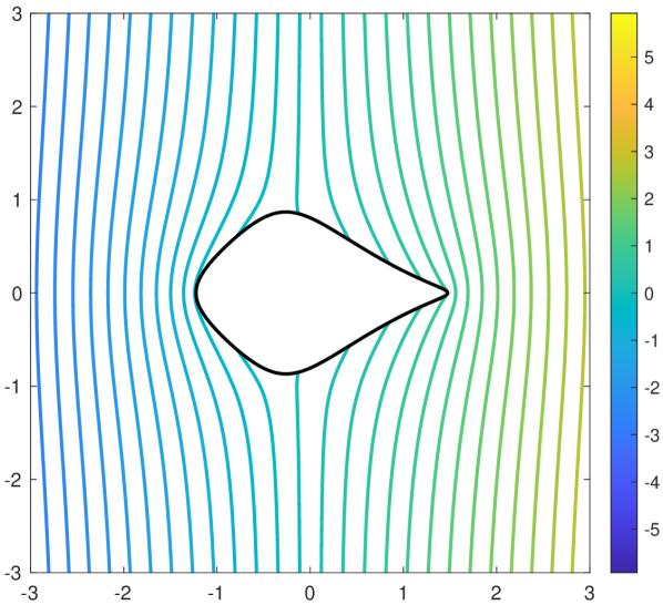
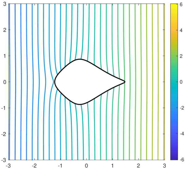
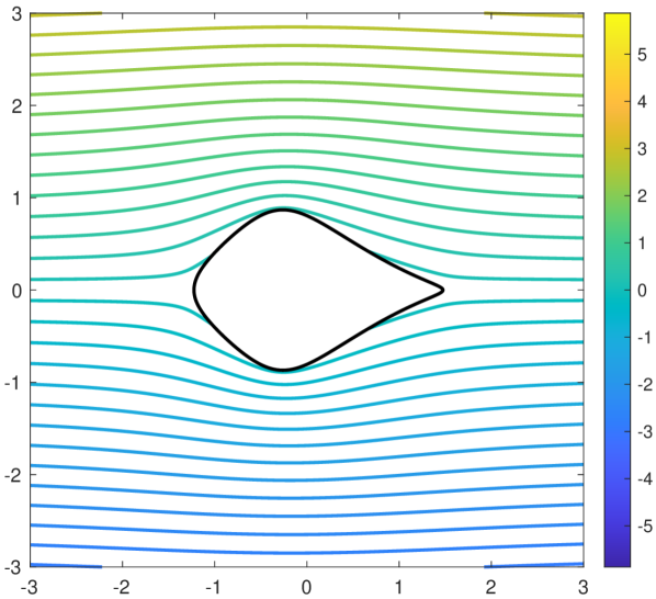
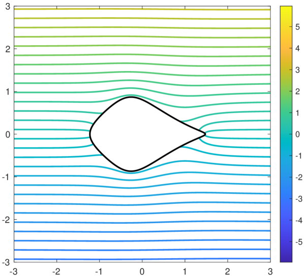
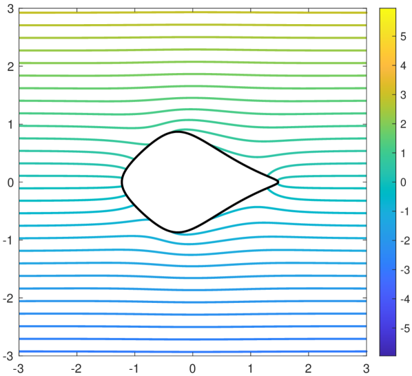
Figure 5.1: The background field is given by $H(x)=x_{1}$. Colored curves represent contours of the potential $u$. We set $\gamma=1$ and the conductivity of the inclusion is given by $\sigma_{c}=5$.

	$\mathbb{N}_{11}^{(1)}$	$\mathbb{N}_{12}^{(1)}$	$\mathbb{N}_{11}^{(2)}$	$\mathbb{N}_{12}^{(2)}$
Perfectly bonding	1.1693	1.0918	7.7190	$-0.7977$
1st order vanishing	$-2.1799\times 10^{-16}$	2.6301	$3.8367\times 10^{-15}$	$-0.1007$
2nd order vanishing	$-3.3353\times 10^{-15}$	$1.7439\times 10^{-16}$	$2.6159\times 10^{-16}$	$2.2846\times 10^{-14}$

Table 1: The leading GPTs for the domains in Figure 5.1.

Example 2.

We now observe a kite-shaped domain with conformal mapping

$$\Psi(w)=w+\frac{0.1}{w}+\frac{0.25}{w^{2}}-\frac{0.05}{w^{3}}+\frac{0.05}{w^{4}}-\frac{0.04}{w^{5}}+\frac{0.02}{w^{6}}.$$

To construct the PT-vanishing structure, we selected values for $P$ based on equation (5.4), where $p_{0}$ is set to $1.4022$ and $p_{2}$ is set to $-0.2742$. For GPTs up to order 2 vanishing structure, we determined the values for $P$ using equation (5.5), with $p_{0}$ set to $1.7975$, $p_{1}$ set to $0.1582$, $p_{2}$ set to $-0.3251$, and $p_{3}$ set to $-1.0352$. Figure 5.2 illustrates the field perturbation under three different boundary conditions.

(a) Perfectly bonding

(b) PT-vanishing

(c) GPT-vanishing up to order 2

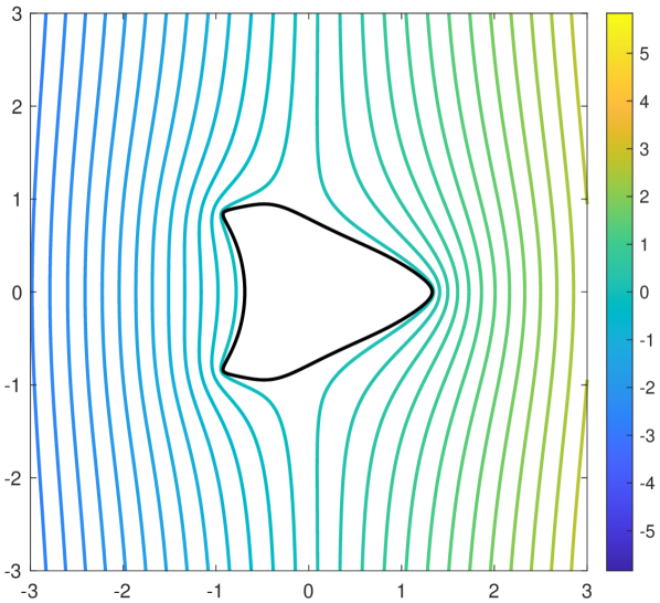
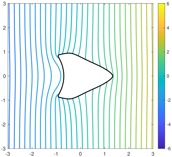
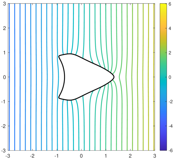
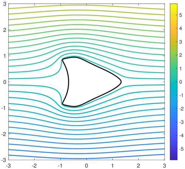
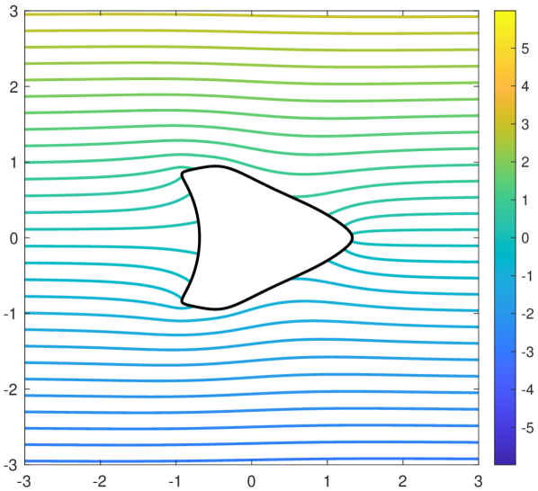
Figure 5.2: The background field is given by $H(x)=x_{1}$ (first row) and $H(x)=x_{2}$ (second row). Colored curves represent contours of the potential $u$. We set $\gamma=1$ and $\sigma_{c}=100$.

	$\mathbb{N}_{11}^{(1)}$	$\mathbb{N}_{12}^{(1)}$	$\mathbb{N}_{11}^{(2)}$	$\mathbb{N}_{12}^{(2)}$
Perfectly bonding	1.2018	5.9817	12.2216	$0.0192$
1st order vanishing	$2.0709\times 10^{-16}$	6.2342	$5.3517\times 10^{-15}$	$0.0085$
2nd order vanishing	$-1.6295\times 10^{-15}$	$-6.7032\times 10^{-15}$	$9.2429\times 10^{-15}$	$-1.1772\times 10^{-15}$

Table 2: The leading GPTs for the domains in Figure 5.2.

6 Conclusion

We propose a novel concept of GPT-vanishing structures for inclusions with arbitrary conductivity and imperfect interfaces. We show that inclusions of general shape can achieve nearly neutral behavior for the background field by carefully selecting a proper imperfect interface parameter. We employ exterior conformal mappings and FPT techniques to compute the coefficients of the interface parameter. Furthermore, we provide two distinct examples that highlight the effect of the vanishing FPTs, demonstrating the practical implications of our proposed concept.

References

- [1] A. Alù and N. Engheta. Achieving transparency with plasmonic and metamaterial coatings. Phys. Rev. - Stat. Nonlinear Soft Matter Phys., 72(1), 2005.
- [2] H. Ammari, J. Garnier, W. Jing, H. Kang, M. Lim, K. Sølna, and H. Wang. Mathematical and statistical methods for multistatic imaging, volume 2098 of Lecture Notes in Mathematics. Springer, Cham, 2013.
- [3] H. Ammari, H. Kang, H. Lee, and M. Lim. Enhancement of near cloaking. Part II: the Helmholtz equation. Commun. Math. Phys., 317(2):485–502, 2013.
- [4] H. Ammari, H. Kang, H. Lee, and M. Lim. Enhancement of near-cloaking using generalized polarization tensors vanishing structures. Part I: The conductivity problem. Commun. Math. Phys., 317(1):253–266, 2013.
- [5] H. Ammari, H. Kang, H. Lee, M. Lim, and S. Yu. Enhancement of near cloaking for the full Maxwell equations. SIAM J. Appl. Math., 73(6):2055–2076, 2013.
- [6] H. Ammari and A. Khelifi. Electromagnetic scattering by small dielectric inhomogeneities. J. Math. Pures Appl., 82(7):749–842, 2003.
- [7] H. Ammari, M. S. Vogelius, and D. Volkov. Asymptotic formulas for perturbations in the electromagnetic fields due to the presence of inhomogeneities of small diameter. II. The full Maxwell equations. J. Math. Pures Appl., 80(8):769–814, 2001.
- [8] Y. Benveniste and T. Miloh. Neutral inhomogeneities in conduction phenomena. J. Mech. Phys. Solids, 47(9):1873–1892, 1999.
- [9] D. Choi, J. Helsing, S. Kang, and M. Lim. Inverse problem for a planar conductivity inclusion. SIAM J. Imag. Sci., to appear.
- [10] D. Choi, J. Kim, and M. Lim. Analytical shape recovery of a conductivity inclusion based on faber polynomials. Math. Ann., 381(3):1837–1867, 2021.
- [11] D. Choi, J. Kim, and M. Lim. Geometric multipole expansion and its application to semi-neutral inclusions of general shape. Z. Angew. Math. Phys., 74(1):39, 2023.
- [12] P. L. Duren. Univalent Functions, volume 259 of Grundlehren der Mathematischen Wissenschaften. Springer-Verlag New York, 1983.
- [13] G. Faber. Über polynomische Entwicklungen. Math. Ann., 57(3):389–408, 1903.
- [14] G. Faber. Über polynomische Entwicklungen II. Math. Ann., 64(1):116–135, 1907.
- [15] T. Feng, H. Kang, and H. Lee. Construction of GPT-vanishing structures using shape derivative. J. Comput. Math., 35(5):569–585, 2017.
- [16] Y. Grabovsky and R. V. Kohn. Microstructures minimizing the energy of a two phase elastic composite in two space dimensions. I: The confocal ellipse construction. J. Mech. Phys. Solids, 43(6):933–947, 1995.
- [17] H. Grunsky. Koeffizientenbedingungen für schlicht abbildende meromorphe Funktionen. Math. Z., 45(1):29–61, 1939.
- [18] Z. Hashin. The elastic moduli of heterogeneous materials. J. Appl. Mech., 29(1):143–150, 1960.
- [19] Z. Hashin. Large isotropic elastic deformation of composites and porous media. Int. J. Solids Struct., 21(7):711–720, 1985.
- [20] Z. Hashin and S. Shtrikman. A variational approach to the theory of the effective magnetic permeability of multiphase materials. J. Appl. Phys., 33(10):3125–3131, 1962.
- [21] P. Jarczyk and V. Mityushev. Neutral coated inclusions of finite conductivity. Proc. R. Soc. A: Math. Phys. Eng. Sci., 468(2140):954–970, 2012.
- [22] Y.-G. Ji, H. Kang, X. Li, and S. Sakaguchi. Neutral Inclusions, Weakly Neutral Inclusions, and an Over-determined Problem for Confocal Ellipsoids, pages 151–181. Springer International Publishing, Cham, 2021.
- [23] S. Jiménez, B. Vernescu, and W. Sanguinet. Nonlinear neutral inclusions: Assemblages of spheres. Int. J. Solids Struct., 50(14-15):2231–2238, 2013.
- [24] Y. Jung and M. Lim. Series Expansions of the Layer Potential Operators Using the Faber Polynomials and Their Applications to the Transmission Problem. SIAM J. Math. Anal., 53(2):1630–1669, 2021.
- [25] H. Kang and H. Lee. Coated inclusions of finite conductivity neutral to multiple fields in two-dimensional conductivity or anti-plane elasticity. Eur. J. Appl. Math., 25(3):329–338, 2014.
- [26] H. Kang, H. Lee, and S. Sakaguchi. An over-determined boundary value problem arising from neutrally coated inclusions in three dimensions. Ann. Sc. Norm. Super. Pisa - Cl. Sci., 16(4):1193–1208, 2016.
- [27] H. Kang and X. Li. Construction of weakly neutral inclusions of general shape by imperfect interfaces. SIAM J. Appl. Math., 79(1):396–414, 2019.
- [28] H. Kang, X. Li, and S. Sakaguchi. Existence of weakly neutral coated inclusions of general shape in two dimensions. Appl. Anal., 101(4):1330–1353, 2022.
- [29] M. Kerker. Invisible bodies. J. Opt. Soc. Am., 65(4):376–379, 1975.
- [30] N. Landy and D. R. Smith. A full-parameter unidirectional metamaterial cloak for microwaves. Nat. Mater., 12(1):25–28, 2013.
- [31] M. Lim and G. W. Milton. Inclusions of general shapes having constant field inside the core and nonelliptical neutral coated inclusions with anisotropic conductivity. SIAM J. Appl. Math., 80(3):1420–1440, 2020.
- [32] H. Liu, Y. Wang, and S. Zhong. Nearly non-scattering electromagnetic wave set and its application. Z. Angew. Math. Phys., 68(2):35, 2017.
- [33] G. W. Milton. The Theory of Composites, volume 6 of Cambridge Monographs on Applied and Computational Mathematics. Cambridge University Press, Cambridge, 2002.
- [34] G. W. Milton and S. K. Serkov. Neutral coated inclusions in conductivity and anti-plane elasticity. Proc. R. Soc. A: Math. Phys. Eng. Sci., 457(2012):1973–1997, 2001.
- [35] D. C. Pham. Solutions for the conductivity of multi-coated spheres and spherically symmetric inclusion problems. Z. Angew. Math. Phys., 69(1):13, 2018.
- [36] D. C. Pham and T. K. Nguyen. The microscopic conduction fields in the multi-coated sphere composites under the imposed macroscopic gradient and flux fields. Z. Angew. Math. Phys., 70(1):24, 2019.
- [37] C.-Q. Ru. Interface design of neutral elastic inclusions. Int. J. Solids Struct., 35(7):559–572, 1998.
- [38] M. Schiffer and G. Szegő. Virtual mass and polarization. Trans. Amer. Math. Soc., 67:130–205, 1949.
- [39] A. Sihvola. On the dielectric problem of isotrophic sphere in anisotropic medium. Electromagnetics, 17(1):69–74, 1997.
- [40] A. Sihvola. Electromagnetic Mixing Formulas and Applications, volume 47 of Electromagnetic Waves. Institution of Engineering and Technology, 1999.
- [41] S. Torquato and M. D. Rintoul. Effect of the interface on the properties of composite media. Phys. Rev. Lett., 75:4067–4070, Nov 1995.
- [42] M. S. Vogelius and D. Volkov. Asymptotic formulas for perturbations in the electromagnetic fields due to the presence of inhomogeneities of small diameter. Math. Model. Numer. Anal., 34(4):723–748, 2000.
- [43] X. Wang and P. Schiavone. A neutral multi-coated sphere under non-uniform electric field in conductivity. Z. Angew. Math. Phys., 64(3):895–903, 2013.
- [44] X. Zhou and G. Hu. Design for electromagnetic wave transparency with metamaterials. Phys. Rev. - Stat. Nonlinear Soft Matter Phys., 74(2), 2006.
- [45] X. Zhou and G. Hu. Acoustic wave transparency for a multilayered sphere with acoustic metamaterials. Phys. Rev. - Stat. Nonlinear Soft Matter Phys., 75(4), 2007.
- [46] X. Zhou, G. Hu, and T. Lu. Elastic wave transparency of a solid sphere coated with metamaterials. Phys. Rev. B - Condens. Matter Mater. Phys., 77(2), 2008.