Charged Anisotropic Models with Complexity-free Condition

Abstract

This paper uses the definition of complexity for a static spherically symmetric spacetime and extends it to the case of charged distribution. We formulate the Einstein-Maxwell field equations corresponding to the anisotropic interior and calculate two different mass functions. We then take Reissner-Nordström metric as an exterior spacetime to find the matching conditions at the spherical boundary. Some scalars are developed from the orthogonal splitting of the curvature tensor, and we call one of them, i.e., $\mathcal{Y}_{TF}$ as the complexity factor for the considered setup. Further, the three independent field equations are not enough to close the system, therefore, we adopt the complexity-free condition. Along with this condition, we consider three constraints that lead to different models. We also present the graphical interpretation of the resulting solutions by choosing some particular values of parameters. We conclude that the models corresponding to $p_{r}=0$ and a polytropic equation of state show viable and stable behavior everywhere.

Keywords: Interior solutions; Vanishing complexity; Relativistic fluids.
PACS: 04.20.Jb; 04.40.-b.; 04.40.Dg.

1 Introduction

General theory of relativity ($\mathbb{GR}$) is regarded as the most acceptable theory in the scientific community among all theories to describe the gravitational field. The corresponding field equations establish a relationship between the geometry of spacetime structure and matter distribution, explained by the Einstein tensor and the energy-momentum tensor ($\mathbb{EMT}$), respectively. This set of differential equations can be solved either analytically or numerically (initial and boundary conditions are needed in this case) according to the situation under consideration. Despite this, it is necessary to provide some extra information associated with the local physics to solve such a system. According to some recent developments [1]-[3], several physical phenomena have been observed while studying compact structures that may cause to deviate the isotropy and local pressure anisotropy inside those systems. Furthermore, there exist multiple factors such as inhomogeneous density, shear and dissipation, etc., which make the isotropic pressure condition unstable [4].

In this context, the field equations provide a set of three independent differential equations for anisotropic sphere, engaging five unknowns (metric potentials and matter functions). Therefore, it is essential to provide two extra conditions in terms of an experiential assumption comprising any physical parameter, or an equation of state to find their solution [5, 6]. In particular, various authors considered a polytropic equation of state [7, 8] to explore physical attributes of a white dwarf [9]. This study has been generalized for the case of anisotropic spherical systems in the framework of $\mathbb{GR}$ [10]-[14]. On the other hand, the metric potentials have been restricted by applying some constraints on them such as the Karmarkar condition in which one of the functions is arbitrarily chosen to generate the total solution [15]-[20]. An alternate condition to this is taken as the conformally flat spacetime, leading to the disappearing Weyl tensor [21]. The whole analysis manifests that the evolution of the fluid distribution inside a self-gravitating body can be characterized by a class of scenarios described by multiple constraints.

In this regard, a most relevant and widely known concept in the field of astronomy is the complexity that can be adopted to study a celestial object. The concept of complexity is related to several physical quantities such as density, heat flux and pressure, etc., that make the interior distribution more complex. Several attempts have been made in multiple disciplines to define this intuitive notion in terms of aforementioned parameters. Firstly, an un-unifying definition of complexity was proposed associated with entropy and data information [22]-[24]. This idea was initially applied on two physical systems, namely ideal gas and a perfect crystal. They were observed to be opposite in their characteristics, however, treated as the complexity-free systems, resulting in the failure of this definition.

A comprehensive definition of complexity was recently given by Herrera [25] in terms of density inhomogeneity and anisotropic pressure. He obtained some scalars by splitting the curvature tensor orthogonally [26, 27] and observed that the above two parameters are involved in a factor $\mathcal{Y}_{TF}$, thus named it complexity factor for a static spherical geometry. The basic idea was that the complexity vanishes either for an isotropic and homogeneous configuration, or if the effects of anisotropy and density inhomogeneity cancel each other. Later, this concept has been generalized to different scenarios (such as static, dynamical and axially symmetric geometries) to study their corresponding different evolutionary patterns [28, 29].

Different evolutionary patterns of celestial structures can efficiently be studied in the presence of electric charge. The matter source influenced from an electromagnetic field creates a force in outward direction that counterbalances the inward directed gravitational pull of a compact star. Consequently, such systems maintain their stability for a longer time as compared to the uncharged stars. The solutions to Einstein-Maxwell field equations and an impact of charge on them have been analyzed [30]-[35]. Sunzu et al. [36] calculated a mass to radius relation for a compact strange star and studied how the presence of charge affects the considered setup. Murad [37] also explored the effect of an electromagnetic field on the developed spherically symmetric model. Sharif and his collaborators [38, 39] formulated decoupled anisotropic charged solutions and found their stable regions.

This paper extends the developed anisotropic spherical models [40] to the case of charged matter distribution. We organize this paper as follows. Section 2 provides $\mathbb{EMT}$ corresponding to anisotropic fluid and the electromagnetic field, and formulates Einstein-Maxwell field equations for spherical interior. The junction conditions are also determined by smoothly matching the interior spacetime with the Reissner-Nordström exterior metric at the boundary. The structure scalars are then presented in section 3, from which we choose $\mathcal{Y}_{TF}$ as the complexity factor for the considered scenario. Section 4 displays a brief summary of some conditions that should be satisfied by a physically realistic model. Furthermore, we present three different models along with their graphical interpretation in section 5. Lastly, we sum up our findings in the last section.

2 Spherical System and Einstein-Maxwell Field Equations

This section presents the field equations characterizing a static charged spherically symmetric fluid configuration. In this regard, we consider a line element representing inner configuration, which is bounded by a spherical surface $\Sigma$ as

$$ds^{2}=-e^{\beta_{1}}dt^{2}+e^{\beta_{2}}dr^{2}+r^{2}d\theta^{2}+r^{2}\sin^{2}\theta d\vartheta^{2},$$ (1)

where $\beta_{1}=\beta_{1}(r)$ and $\beta_{2}=\beta_{2}(r)$. This metric must satisfy Einstein-Maxwell field equations given in the following form

$$\mathbb{G}_{\zeta\delta}=8\pi\big{(}\mathbb{T}_{\zeta\delta}+\mathbb{E}_{\zeta\delta}\big{)},$$ (2)

where $\mathbb{G}_{\zeta\delta},~{}\mathbb{T}_{\zeta\delta}$ and $\mathbb{E}_{\zeta\delta}$ describe the Einstein tensor, $\mathbb{EMT}$ for the matter source and the electromagnetic field, respectively. The $\mathbb{EMT}$ representing anisotropic fluid configuration has the form

$$\mathbb{T}_{\zeta\delta}=(\rho+p_{t})\mathcal{K}_{\zeta}\mathcal{K}_{\delta}+p_{t}g_{\zeta\delta}+\left(p_{r}-p_{t}\right)\mathcal{W}_{\zeta}\mathcal{W}_{\delta},$$ (3)

where $\rho,~{}p_{r},~{}p_{t},~{}\mathcal{W}_{\delta}$ and $\mathcal{K}_{\delta}$ symbolize the energy density, radial/tangential pressure, four-vector and four-velocity, respectively. These quantities take the form for the line element (1) as

$$\mathcal{W}^{\delta}=(0,e^{\frac{-\beta_{2}}{2}},0,0),\quad\mathcal{K}^{\delta}=(e^{\frac{-\beta_{1}}{2}},0,0,0),$$ (4)

which satisfy the relations $\mathcal{W}^{\delta}\mathcal{K}_{\delta}=0,~{}\mathcal{W}^{\delta}\mathcal{W}_{\delta}=1$ and $\mathcal{K}^{\delta}\mathcal{K}_{\delta}=-1$.

The electromagnetic field can be characterized by $\mathbb{EMT}$ as

$$\mathbb{E}_{\zeta\delta}=-\frac{1}{4\pi}\left[\frac{1}{4}g_{\zeta\delta}\mathbb{F}^{\mu\sigma}\mathbb{F}_{\mu\sigma}-\mathbb{F}^{\sigma}_{\zeta}\mathbb{F}_{\delta\sigma}\right].$$ (5)

Here, $\mathbb{F}_{\mu\sigma}=\psi_{\sigma;\mu}-\psi_{\mu;\sigma}$ is the Maxwell field tensor and $\psi_{\sigma}=\psi(r)\delta^{0}_{\sigma}$ represents the four-potential. The Maxwell equations satisfied by these entities can be expressed in tensorial form as

$$\mathbb{F}^{\mu\sigma}_{;\sigma}=4\pi\jmath^{\mu},\quad\mathbb{F}_{[\mu\sigma;\zeta]}=0,$$

where $\jmath^{\mu}=\varrho\mathcal{K}^{\mu}$, $\jmath^{\mu}$ and $\varrho$ are the current and charge densities, respectively. These equations become in the current scenario as

$$\psi^{\prime\prime}+\frac{1}{2r}\big{\{}4-r(\beta_{1}^{\prime}+\beta_{2}^{\prime})\big{\}}\psi^{\prime}=4\pi\varrho e^{\frac{\beta_{1}}{2}+\beta_{2}},$$ (6)

where ${}^{\prime}=\frac{\partial}{\partial r}$. By integrating the above equation, we have

$$\psi^{\prime}=\frac{s}{r^{2}}e^{\frac{\beta_{1}+\beta_{2}}{2}}.$$ (7)

Here, $s=\int_{0}^{r}\varrho e^{\frac{\beta_{2}}{2}}\bar{r}^{2}d\bar{r}$ demonstrates the total charge inside spherical geometry (1). The non-vanishing components of $\mathbb{EMT}s$ (3) and (5) are

$$\mathbb{T}_{00}=\rho e^{\beta_{1}},\quad\mathbb{T}_{11}=p_{r}e^{\beta_{2}},\quad\mathbb{T}_{22}=p_{t}r^{2}=\frac{\mathbb{T}_{33}}{sin^{2}\theta},$$

$$\mathbb{E}_{00}=\frac{s^{2}e^{\beta_{1}}}{8\pi r^{4}},\quad\mathbb{E}_{11}=-\frac{s^{2}e^{\beta_{2}}}{8\pi r^{4}},\quad\mathbb{E}_{22}=\frac{s^{2}}{8\pi r^{2}}=\frac{\mathbb{E}_{33}}{sin^{2}\theta}.$$

The Einstein-Maxwell field equations (2) for spherical model (1) are calculated as

$$8\pi\rho+\frac{s^{2}}{r^{4}} =\frac{1}{r^{2}}-e^{-\beta_{2}}\left(\frac{1}{r^{2}}-\frac{\beta_{2}^{\prime}}{r}\right),$$ (8)

$$8\pi{p}_{r}-\frac{s^{2}}{r^{4}} =e^{-\beta_{2}}\left(\frac{1}{r^{2}}+\frac{\beta_{1}^{\prime}}{r}\right)-\frac{1}{r^{2}},$$ (9)

$$8\pi{p}_{t}+\frac{s^{2}}{r^{4}} =\frac{e^{-\beta_{2}}}{4}\left[\beta_{1}^{\prime 2}-\beta_{1}^{\prime}\beta_{2}^{\prime}+2\beta_{1}^{\prime\prime}-\frac{2\beta_{2}^{\prime}}{r}+\frac{2\beta_{1}}{r}\right].$$ (10)

The hydrostatic equilibrium condition (developed from the conservation law, i.e., $\nabla_{\zeta}(\mathbb{T}^{\zeta\delta}+\mathbb{E}^{\zeta\delta})=0$) becomes

$$\frac{dp_{r}}{dr}+\frac{\beta_{1}^{\prime}}{2}\big{(}\rho+p_{r}\big{)}-\frac{2}{r}\big{(}p_{t}-p_{r}\big{)}-\frac{ss^{\prime}}{4\pi r^{4}}=0,$$ (11)

which is also known as the generalized Tolman-Opphenheimer-Volkoff ($\mathcal{TOV}$) equation for charged anisotropic matter distribution. The mass function in this case becomes

$$m(r)=\frac{r}{2}\bigg{(}1-e^{\beta_{2}}+\frac{s^{2}}{r^{2}}\bigg{)},$$ (12)

or in terms of the energy density, it takes the form after combining with Eq.(8) as

$$m(r) =4\pi\int_{0}^{r}\rho\bar{r}^{2}d\bar{r}+\int_{0}^{r}\frac{ss^{\prime}}{\bar{r}}d\bar{r}$$

$$=4\pi\int_{0}^{r}\rho\bar{r}^{2}d\bar{r}+\frac{1}{2}\int_{0}^{r}\frac{s^{2}}{\bar{r}^{2}}d\bar{r}+\frac{s^{2}}{2r}.$$ (13)

Equation (9) provides the value of differential of temporal metric potential in terms of the mass (12) as

$$\beta_{1}^{\prime}=\frac{2\big{(}4\pi p_{r}r^{4}+mr-s^{2}\big{)}}{r\big{(}r^{2}-2mr+s^{2}\big{)}},$$ (14)

which after substitution in Eq.(11) yields

$$\frac{dp_{r}}{dr}+\frac{\big{(}4\pi p_{r}r^{4}+mr-s^{2}\big{)}}{r\big{(}r^{2}-2mr+s^{2}\big{)}}\big{(}\rho+p_{r}\big{)}+\frac{2\Pi}{r}-\frac{ss^{\prime}}{4\pi r^{4}}=0,$$ (15)

where the anisotropic factor is defined as $\Pi=p_{r}-p_{t}$.

Since the interior distribution is influenced from the electromagnetic field, so the most suitable geometry representing the exterior spacetime is the Reissner-Nordström solution given by

$$ds^{2}=-\bigg{(}1-\frac{2\bar{\mathcal{M}}}{r}+\frac{\bar{\mathcal{S}}^{2}}{r^{2}}\bigg{)}dt^{2}+\bigg{(}1-\frac{2\bar{\mathcal{M}}}{r}+\frac{\bar{\mathcal{S}}^{2}}{r^{2}}\bigg{)}^{-1}dr^{2}+r^{2}d\theta^{2}+r^{2}\sin^{2}\theta d\vartheta^{2},$$ (16)

where $\bar{\mathcal{M}}$ and $\bar{\mathcal{S}}$ are the total mass and charge of the exterior. The continuity of fundamental forms of the matching conditions at the boundary ($r=r_{\Sigma}=\mathcal{R}$) yields

$$e^{\beta_{1}} {{}_{=}^{\Sigma}}1-\frac{2\bar{\mathcal{M}}}{\mathcal{R}}+\frac{\bar{\mathcal{S}}^{2}}{\mathcal{R}^{2}},$$ (17)

$$e^{-\beta_{2}} {{}_{=}^{\Sigma}}1-\frac{2\bar{\mathcal{M}}}{\mathcal{R}}+\frac{\bar{\mathcal{S}}^{2}}{\mathcal{R}^{2}},$$ (18)

$$p_{r} {{}_{=}^{\Sigma}}0,\quad s{{}_{=}^{\Sigma}}\bar{\mathcal{S}}.$$ (19)

Equations (17)-(19) play highly significant role such that the smooth matching between the metrics (1) and (16) would not be possible without taking them into the account.

3 Structure Scalars and Complexity of Compact Sources

The concept of the complexity of a self-gravitating system has become a topic of great interest in the field of astrophysics. Among several definitions of the complexity in the literature, it was proposed that a structure having isotropic and homogeneous distribution must have a zero complexity. In the light of this, one can think that a complexity factor in fact measures how the inhomogeneous density and pressure anisotropy are related to each other. A definition in terms of these two factors was firstly proposed by Herrera [25] by splitting the Riemann tensor orthogonally [26, 27], and then chosen one of the resulting scalars as the complexity factor. This section briefly discusses the procedure to obtain the complexity factor that associates with different physical parameters. The Riemann tensor can be split into its trace and trace-free parts through the following equation as

$$\mathbb{R}^{\zeta\varphi}_{\delta\vartheta}=\mathbb{C}^{\zeta\varphi}_{\delta\vartheta}+16\pi\big{(}\mathbb{T}^{[\zeta}_{[\delta}\delta^{\varphi]}_{\vartheta]}+\mathbb{E}^{[\zeta}_{[\delta}\delta^{\varphi]}_{\vartheta]}\big{)}+8\pi\mathbb{T}\left(\frac{1}{3}\delta^{\zeta}_{[\delta}\delta^{\varphi}_{\vartheta]}-\delta^{[\zeta}_{[\delta}\delta^{\varphi]}_{\vartheta]}\right),$$ (20)

and the two tensors such as $\mathcal{Y}_{\varphi\vartheta}$ and $\mathcal{X}_{\varphi\vartheta}$ are defined by

$$\mathcal{Y}_{\zeta\delta} = \mathcal{R}_{\zeta\varphi\delta\vartheta}\mathcal{K}^{\varphi}\mathcal{K}^{\vartheta},$$ (21)

$$\mathcal{X}_{\zeta\delta} = {}^{\ast}\mathcal{R}^{\ast}_{\zeta\varphi\delta\vartheta}\mathcal{K}^{\varphi}\mathcal{K}^{\vartheta}=\frac{1}{2}\eta^{\omega\sigma}_{\zeta\varphi}\mathcal{R}^{\ast}_{\omega\sigma\delta\vartheta}\mathcal{K}^{\varphi}\mathcal{K}^{\vartheta},$$ (22)

where $\mathcal{R}^{\ast}_{\zeta\varphi\delta\vartheta}=\frac{1}{2}\eta_{\omega\sigma\delta\vartheta}\mathcal{R}^{\omega\sigma}_{\zeta\varphi}$ and $\eta^{\omega\sigma}_{\zeta\varphi}$ is the Levi-Civita symbol. These tensors can alternatively be expressed in terms of trace $(\mathcal{Y}_{T},~{}\mathcal{X}_{T})$ and trace-free parts $(\mathcal{Y}_{TF},~{}\mathcal{X}_{TF})$ as

$$\mathcal{Y}_{\zeta\delta} = \frac{h_{\zeta\delta}\mathcal{Y}_{T}}{3}+\bigg{(}\mathcal{W}_{\zeta}\mathcal{W}_{\delta}-\frac{h_{\zeta\delta}}{3}\bigg{)}\mathcal{Y}_{TF},$$ (23)

$$\mathcal{X}_{\zeta\delta} = \frac{h_{\zeta\delta}\mathcal{X}_{T}}{3}+\bigg{(}\mathcal{W}_{\zeta}\mathcal{W}_{\delta}-\frac{h_{\zeta\delta}}{3}\bigg{)}\mathcal{X}_{TF}.$$ (24)

Here, $h_{\zeta\delta}=g_{\zeta\delta}+\mathcal{K}_{\zeta}\mathcal{K}_{\delta}$ is the projection tensor. Using Eqs.(20)-(24) and after some manipulation, we obtain the following scalars as

$$\mathcal{X}_{T}=8\pi\rho+\frac{s^{2}}{r^{4}},$$ (25)

$$\mathcal{X}_{TF}=-\mathcal{E}-4\pi\Pi+\frac{s^{2}}{r^{4}},$$ (26)

$$\mathcal{Y}_{T}=4\pi\big{(}\rho+3p_{r}-2\Pi\big{)}+\frac{s^{2}}{r^{4}},$$ (27)

$$\mathcal{Y}_{TF}=\mathcal{E}-4\pi\Pi+\frac{s^{2}}{r^{4}},$$ (28)

where the electric part of the Weyl tensor is is defined by

$$\mathcal{E}=\frac{e^{-\beta_{2}}}{4}\left[\beta_{1}^{\prime\prime}+\frac{\beta_{1}^{\prime 2}-\beta_{2}^{\prime}\beta_{1}^{\prime}}{2}-\frac{\beta_{1}^{\prime}-\beta_{2}^{\prime}}{r}+\frac{2(1-e^{\beta_{2}})}{r^{2}}\right].$$ (29)

These scalar functions are associated with physical attributes of a self-gravitating structure such as homogeneous/inhomogeneous energy density and anisotropic pressure. Since our goal is to choose the complexity factor from the above four scalars, so the following form of $\mathcal{Y}_{TF}$ (28) indicates that only this factor involves all the required parameters, given by

$$\mathcal{Y}_{TF}=\frac{4\pi}{r^{3}}\int_{0}^{r}\bar{r}^{3}\rho^{\prime}d\bar{r}-\frac{3}{r^{3}}\int_{0}^{r}\frac{ss^{\prime}}{\bar{r}}d\bar{r}-8\pi\Pi+\frac{2s^{2}}{r^{4}}.$$ (30)

This factor disappears for the isotropic and homogeneous configuration in the absence of charge. Further, the Tolman (or active gravitational) mass [41] is referred as

$$m_{T}=4\pi\int_{0}^{r}\bar{r}^{2}e^{(\beta_{1}+\beta_{2})/2}(-\mathbb{T}^{0}_{0}-\mathbb{E}^{0}_{0}+\mathbb{T}^{1}_{1}+\mathbb{E}^{1}_{1}+2\mathbb{T}^{2}_{2}+2\mathbb{E}^{2}_{2})d\bar{r},$$ (31)

which helps to explain the energy of the fluid distribution. Equation (31) yields an alternative expression, after some calculations, as

$$m_{T} =(m_{T})_{\Sigma}\bigg{(}\frac{r}{\mathcal{R}}\bigg{)}^{3}+r^{3}\int_{r}^{\mathcal{R}}\frac{e^{(\beta_{1}+\beta_{2})/2}}{\bar{r}^{5}}$$

$$\bigg{\{}4\pi\bar{r}\int_{0}^{r}\tilde{r}^{3}\rho^{\prime}d\tilde{r}-3\bar{r}\int_{0}^{r}\frac{ss^{\prime}}{\tilde{r}}d\tilde{r}-8\pi\bar{r}^{4}\Pi+4s^{2}\bigg{\}}d\bar{r}.$$ (32)

The Tolman mass (32) can also be written in terms of scalar (30) as

$$m_{T} =(m_{T})_{\Sigma}\bigg{(}\frac{r}{\mathcal{R}}\bigg{)}^{3}+r^{3}\int_{r}^{\mathcal{R}}\frac{e^{(\beta_{1}+\beta_{2})/2}}{\bar{r}^{5}}\big{\{}\mathcal{Y}_{TF}\bar{r}^{4}+2s^{2}\big{\}}d\bar{r}.$$ (33)

Equation (33) interprets how the active gravitational mass is influenced by the inhomogeneous density and pressure anisotropy through the function $\mathcal{Y}_{TF}$. It is important to point out here that the complexity-free system is not only characterized by isotropic and homogeneous distribution. Indeed, Eq.(30) also describes such system ($\mathcal{Y}_{TF}=0$) only if the following condition holds

$$\Pi=\frac{1}{2r^{3}}\int_{0}^{r}\bar{r}^{3}\rho^{\prime}d\bar{r}-\frac{3}{8\pi r^{3}}\int_{0}^{r}\frac{ss^{\prime}}{\bar{r}}d\bar{r}+\frac{s^{2}}{4\pi r^{4}},$$ (34)

which implies that there exist a class of solutions satisfying this condition. Since the above condition provides a non-local equation of state, thus this would be very helpful in constructing the solutions to the field equations (2).

4 Some Physical Conditions for the Acceptance of Realistic Models

Numerous strategies have been found in the literature to solve the field equations describing physically acceptable compact objects. However, if these solutions fail to satisfy acceptability conditions, they are no more relevant to model real compact systems. Multiple conditions in this regard have been proposed and complied by various authors [42, 43]. Some of them are highlighted in the following.

• In the interior of a self-gravitating star, the behavior of radial and temporal metric functions must be finite, singularity-free and positive.

• The matter variables (energy density and pressure) must be finite and maximum at the core ($r=0$) and positive in the whole domain. Moreover, their derivatives should be zero at $r=0$ and negative towards the boundary to show monotonically decreasing trend.

• For the charged system, the compactness is given by

  $$\mathcal{R}-\sqrt{\mathcal{R}^{2}-2\mathcal{\bar{M}}\mathcal{R}+\mathcal{\bar{S}}^{2}}-\bigg{(}\mathcal{M}-\frac{\mathcal{\bar{S}}^{2}}{2\mathcal{R}}\bigg{)}\leq\frac{1}{2}\bigg{(}\mathcal{\bar{M}}-\frac{\mathcal{\bar{S}}^{2}}{2\mathcal{R}}\bigg{)},$$

  where $\mathcal{\bar{M}}-\frac{\mathcal{\bar{S}}^{2}}{2\mathcal{R}}\neq 0$. The analogous definition of compactness in this case becomes

  $$\frac{\mathcal{\bar{M}}}{\mathcal{R}}\leq\frac{8}{9}\bigg{\{}\frac{1}{1+\sqrt{1-\frac{8\gamma^{2}}{9}}}\bigg{\}},\quad\gamma^{2}=\frac{\mathcal{\bar{S}}^{2}}{\mathcal{\bar{M}}^{2}}.$$

  Equivalently, we have [44, 45]

  $$\frac{1}{\mathcal{R}}\bigg{(}2\mathcal{\bar{M}}-\frac{\mathcal{\bar{S}}^{2}}{\mathcal{R}}\bigg{)}\leq\frac{8}{9}.$$ (35)

• The presence of ordinary matter in the interior of a celestial body can be guaranteed by satisfying some constraints imposed on $\mathbb{EMT}$, named as the energy conditions. They have the following form in the current setup

  $$\rho\geq 0,\quad\rho+p_{r}\geq 0,$$

  $$\rho+p_{t}\geq 0,\quad\rho-p_{r}\geq 0,$$

  $$\rho-p_{t}\geq 0,\quad\rho+p_{r}+2p_{t}\geq 0.$$ (36)

  The most essential bounds among all the above conditions to be fulfilled are the dominant energy conditions (i.e., $\rho-p_{r}$ and $\rho-p_{t}$), which claim $\rho\geq p_{r}$ and $\rho\geq p_{t}$ everywhere.

• The redshift for the interior configuration is defined as $Z=e^{-\beta_{1}/2}-1$. Since this factor depends only on the temporal metric potential, thus it must decrease towards the boundary. Also, its value must be less than or equal to $5.211$ at $\Sigma$ to get an acceptable model [46].

• To check the stability of a celestial system just departed from hydrostatic equilibrium has become a topic of great interest now a days. Herrera et al. [47, 48] discussed the notion of cracking which occurs inside the fluid when sign of the total radial force changes at some particular point. The cracking can be avoided if the following inequality holds

  $$-1\leq v_{st}^{2}-v_{sr}^{2}\leq 0,$$ (37)

  where $v_{sr}^{2}=\frac{dp_{r}}{d\rho}$ and $v_{st}^{2}=\frac{dp_{t}}{d\rho}$ are the radial and tangential sound speeds, respectively.

5 Models

There are multiple possible models suggested by different authors to calculate solutions of the field equations. For example, Herrera [25] formulated such solutions by considering two constraints like the Gokhroo and Mehra ansatz and the polytropic equation along with vanishing complexity factor. Among all the conditions, we adopt three different models and analyze physical characteristics of the corresponding developed solutions in the following subsections.

5.1 Complexity-free Condition with $p_{r}=0$ Case

The field equations (8)-(10) contain six unknowns ($\rho,p_{r},p_{t},\beta_{1},\beta_{2},s$), thus we shall require to take some extra constraints to find their solution. We adopt the known form of the charge [49] to reduce one degree of freedom, that is why we are left with five unknowns to be calculated. For this, we consider $\mathcal{Y}_{TF}=0$ and $p_{r}=0$ constraints which represent a spherical solution characterized only by the tangential pressure due to Florides [50]. The later condition provides from Eq.(9) as

$$e^{\beta_{2}}=\frac{r^{2}\big{(}1+\beta_{1}^{\prime}r\big{)}}{r^{2}-s^{2}}.$$ (38)

Inserting Eqs.(8), (10) and (38) into (34), we obtain a second order differential equation for $\beta_{1}$ as

$$r\beta_{1}^{\prime}\big{(}s^{4}-2r^{3}(12\mathcal{Q}+r)-5s^{2}r^{2}+\big{(}r^{6}-s^{2}r^{4}\big{)}\beta_{1}^{\prime\prime}\big{)}-2r^{5}(6\mathcal{Q}+r)\beta_{1}^{\prime 2}$$

$$-12\mathcal{Q}r^{3}+s^{4}-5s^{2}r^{2}+\big{(}r^{7}-s^{2}r^{5}\big{)}\beta_{1}^{\prime 3}+\big{(}2r^{6}-2s^{2}r^{4}\big{)}\beta_{1}^{\prime\prime}=0,$$ (39)

where $\mathcal{Q}=\int_{0}^{r}\frac{ss^{\prime}}{r}dr$.

Equation (39) can only be integrated through numerical technique, whose solution along with (38) make both the metric coefficients known. Figure 1 exhibits the plots of metric potentials $e^{\beta_{1}}$ and $e^{-\beta_{2}}$ whose behavior is positive, singularity-free and finite everywhere. Moreover, we observe that these functions attain expected values at the center, as $e^{\beta_{1}(0)}=\mathcal{C}$ (where $\mathcal{C}$ is a positive constant) and $e^{-\beta_{2}(0)}=1$. The radius of the surface of a star is a point where these potentials coincide. In this case, we find that they coincide at $\mathcal{R}\approx 0.12$, so that the matching conditions give

$$e^{\beta_{1}(0.12)}=e^{-\beta_{2}(0.12)}\approx 0.87=1-\frac{2\mathcal{\bar{M}}}{\mathcal{R}}+\frac{\mathcal{\bar{S}}^{2}}{\mathcal{R}^{2}},$$

which provides compactness of the current structures as

$$\frac{2\mathcal{\bar{M}}}{\mathcal{R}}-\frac{\mathcal{\bar{S}}^{2}}{\mathcal{R}^{2}}\approx 0.13<\frac{8}{9}.$$ (40)

Figure 2 (left plot) presents the behavior of energy density which is maximum at $r=0$ and decreases towards the hypersurface. Furthermore, the presence of charge makes the system less dense as compared to the uncharged configuration. Since the system with vanishing radial pressure is related to Florides solution, therefore the spherical stability can only be preserved if the tangential pressure has a positive and increasing behavior outwards. Figure 2 (right plot) shows the trend of $p_{t}$ that is consistent with the required result. The nature of anisotropy is observed to be zero at the core and opposite from the tangential pressure towards the boundary (lower plot).

The energy conditions are plotted in Figure 3 that provide acceptable behavior, resulting in the viability of this solution. Figure 4 (left) manifests the interior redshift that decreases with increases $r$, and its value at the surface is found as $Z(0.12)\approx 0.96$. This value is much less than its observed upper limit, i.e., $Z_{\mathcal{R}}=5.211$. The stability is also checked in Figure 4 (right) from which we notice that the developed model, in this case, avoids cracking and retains stability everywhere.

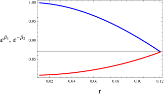
Figure 1: Plots of $e^{\beta_{1}}$ (red) and $e^{-\beta_{2}}$ (blue) corresponding to Model I.

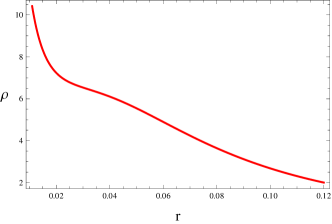
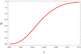
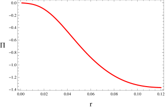
Figure 2: Plots of energy density, tangential pressure and anisotropy corresponding to Model I.

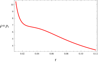
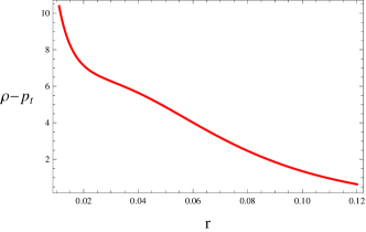
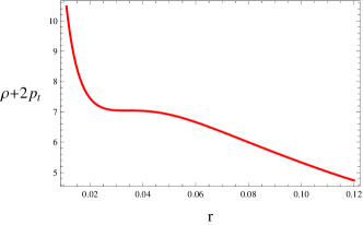
Figure 3: Plots of energy conditions corresponding to Model I.

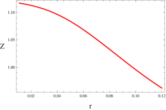
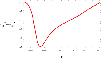
Figure 4: Plots of redshift and cracking condition corresponding to Model I.

5.2 Complexity-free Polytrope

The polytrope corresponding to anisotropic distribution plays a crucial role in astrophysics and has been discussed thoroughly by various authors [12]-[14]. Since we need two constraints to solve the field equations (8)-(10), thus a polytropic equation of state along with complexity-free condition is taken in this case. A brief discussion was presented on this model in [25], however, we analyze the corresponding solution in more detail through graphical interpretation. We provide the following two conditions to continue our analysis as

$$p_{r}=\mathcal{H}\rho^{\eta}=\mathcal{H}\rho^{1+\frac{1}{\mathcal{N}}},\quad\mathcal{Y}_{TF}=0,$$ (41)

where $\mathcal{H},~{}\mathcal{N}$ and $\eta$ symbolize the polytropic constant, polytropic index and polytropic exponent, respectively.

We now introduce some new variables to convert $\mathcal{TOV}$ equation and the mass function in dimensionless form as

$$\zeta=\frac{p_{rc}}{\rho_{c}},\quad r=\frac{\xi}{\mathcal{B}},\quad\mathcal{B}^{2}=\frac{4\pi\rho_{c}}{\zeta(\mathcal{N}+1)},$$ (42)

$$\Psi^{\mathcal{N}}=\frac{\rho}{\rho_{c}},\quad\nu(\xi)=\frac{\mathcal{B}^{3}m(r)}{4\pi\rho_{c}},$$ (43)

where $c$ in the subscript defines the value of that quantity at the center. At $r=\mathcal{R}$ (or $\xi(r)=\xi(\mathcal{R})$), we have $\Psi\big{(}\xi(\mathcal{R})\big{)}=0$. Equations (13) and (15) can be written after substitution of the above variables as

$$\frac{2\Pi\Psi^{-\mathcal{N}}\xi}{p_{rc}\big{(}\mathcal{N}+1\big{)}\big{(}1+\zeta\Psi\big{)}}\bigg{\{}1-\frac{2(\mathcal{N}+1)\zeta\nu}{\xi}+\frac{4\pi\rho_{c}s^{2}}{\zeta\xi^{2}\big{(}\mathcal{N}+1\big{)}}\bigg{\}}+\frac{\xi^{2}}{1+\zeta\Psi}$$

$$\times\bigg{\{}\frac{d\Psi}{d\xi}-\frac{4\pi\rho_{c}s\Psi^{\mathcal{N}}}{\xi^{4}\zeta^{3}\big{(}\mathcal{N}+1\big{)}^{3}}\frac{ds}{d\xi}\bigg{\}}\bigg{\{}1-\frac{2(\mathcal{N}+1)\zeta\nu}{\xi}+\frac{4\pi\rho_{c}s^{2}}{\zeta\xi^{2}\big{(}\mathcal{N}+1\big{)}}\bigg{\}}$$

$$+\zeta\xi^{3}\Psi^{\mathcal{N}+1}+\nu-\frac{4\pi\rho_{c}s^{2}}{\xi\zeta^{2}\big{(}\mathcal{N}+1\big{)}^{2}}=0,$$ (44)

$$4\pi\rho_{c}\frac{d\nu}{d\xi}=4\pi\rho_{c}\Psi^{\mathcal{N}}\xi^{2}+\frac{ss^{\prime}\mathcal{B}^{3}}{\xi}.$$ (45)

Since there are two first order differential equations (44) and (45) in three variables $\Psi,~{}\nu$ and $\Pi$, thus we need one more equation to find these unknowns. For this purpose, we choose $\mathcal{Y}_{TF}=0$ condition which becomes in terms of variables (42) and (43) as

$$\frac{6\Pi}{\xi}+2\frac{d\Pi}{d\xi}=\rho_{c}\mathcal{N}\Psi^{\mathcal{N}-1}\frac{d\Psi}{d\xi}+\frac{ss^{\prime}\mathcal{B}^{3}}{4\pi\xi^{4}}-\frac{s^{2}\mathcal{B}^{4}}{2\pi\xi^{5}}.$$ (46)

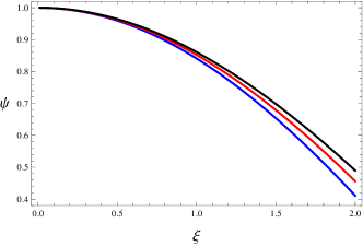
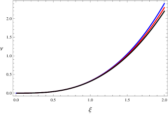
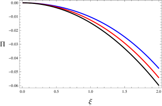
Figure 5: Plots of $\Psi,~{}\nu$ and $\Pi$ for $\zeta=0.1$, $\rho_{c}=1$ and $\mathcal{N}=0.3$ (blue), $\mathcal{N}=0.4$ (red), and $\mathcal{N}=0.5$ (black) corresponding to Model II.

We now have three equations in three unknowns, so a unique solution can be easily obtained by solving them numerically with the following conditions

$$\Pi(0)=0,\quad\nu(0)=0,\quad\Psi(0)=1.$$

We fix the value of $\zeta$ and observe the graphical behavior of the above three unknowns as a function of $\xi$ by varying the parameter $\mathcal{N}$. Figure 5 (left) shows the behavior of $\Psi$ (i.e., energy density) which is maximum at $\xi=0$ and decreases outwards, indicating well-behaved polytropes. The mass of the considered distribution manifests a monotonically increasing trend and we observe it in an inverse relation with $\mathcal{N}$ (right plot). The lower plot exhibits anisotropy which disappears at the core and shows negative behavior towards the surface for all the chosen values of $\mathcal{N}$.

The geometric sector for the solution corresponding to constraints (41) is plotted in Figure 6. We observe the acceptable behavior of both the metric potentials. Moreover, we get $e^{\beta_{1}(0)}=\mathcal{C}$ and $e^{-\beta_{2}(0)}=1$ at $\xi=0$, and they coincide at $\xi=2$ which is the surface of a star. We are now allowed to calculate the compactness factor. For $\mathcal{N}=0.3$, we have

$$e^{\beta_{1}(2)}=e^{-\beta_{2}(2)}\approx 0.61=1-\frac{2\mathcal{\bar{M}}}{\mathcal{R}}+\frac{\mathcal{\bar{S}}^{2}}{\mathcal{R}^{2}},$$

which delivers the compactness as

$$\frac{2\mathcal{\bar{M}}}{\mathcal{R}}-\frac{\mathcal{\bar{S}}^{2}}{\mathcal{R}^{2}}\approx 0.39<\frac{8}{9}.$$ (47)

Figure 7 shows the plots of matter variables such as density and pressure with respect to a new dimensionless coordinate $\xi$ for certain values of parameters in Eqs.(42) and (43). We observe their maximum values at the center and minimum at the boundary following decreasing trend. The radial pressure becomes zero at $\xi=2$ (upper left plot). Although the density is observed to be much greater than radial/tangential pressures, all the energy conditions shown in Figure 8 characterize a viable model.

The interior redshift for this model is displayed in Figure 9 (left), which shows a decreasing trend with the increase in $\xi$. Also at $\xi=2$, its value becomes $Z(2)\approx 1.48<Z_{\mathcal{R}}$, as expected. We also analyze the stable region in the right plot and find that the cracking condition takes negative values everywhere, pointing out the stability of the developed solution unlike the uncharged distribution [40].

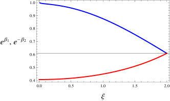
Figure 6: Plots of $e^{\beta_{1}}$ (red) and $e^{-\beta_{2}}$ (blue) for $\zeta=0.1$, $\rho_{c}=1$, $\mathcal{H}=0.9$ and $\mathcal{N}=0.3$ corresponding to Model II.

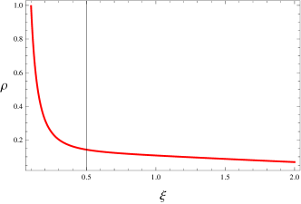
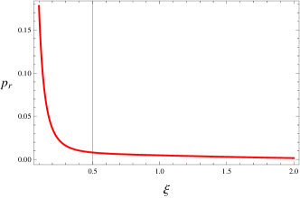
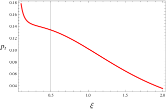
Figure 7: Plots of energy density, radial and tangential pressures for $\zeta=0.1$, $\rho_{c}=1$, $\mathcal{H}=0.9$ and $\mathcal{N}=0.3$ corresponding to Model II.

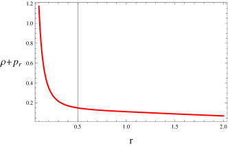
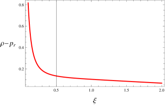
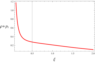
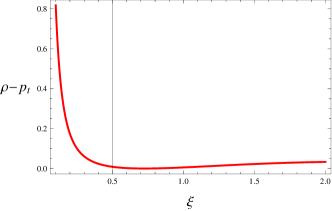
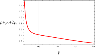
Figure 8: Plots of energy conditions for $\zeta=0.1$, $\rho_{c}=1$, $\mathcal{H}=0.9$ and $\mathcal{N}=0.3$ corresponding to Model II.

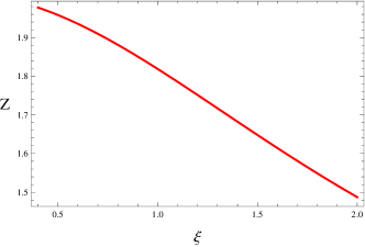
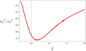
Figure 9: Plots of redshift and cracking condition for $\zeta=0.1$, $\rho_{c}=1$, $\mathcal{H}=0.9$ and $\mathcal{N}=0.3$ corresponding to Model II.

5.3 Complexity-free Condition with a Non-local Equation of State

A non-local equation of state was firstly proposed in [51] to discuss a self-gravitating system. Its expression is given in the following

$$p_{r}=\rho-\frac{2}{r^{3}}\int_{0}^{r}\rho\bar{r}^{2}d\bar{r}+\frac{\mathbb{C}}{2\pi r^{3}},$$ (48)

where $\mathbb{C}$ is a constant. The above equation can be written after using the mass function (13) as

$$p_{r}=\frac{1}{4\pi{r^{2}}}\bigg{(}m^{\prime}-\frac{ss^{\prime}}{r}\bigg{)}-\frac{1}{2\pi{r^{3}}}\bigg{(}m-\int_{0}^{r}\frac{ss^{\prime}}{\bar{r}}d\bar{r}\bigg{)}+\frac{\mathbb{C}}{2\pi r^{3}}.$$ (49)

Equation (49) along with $\mathcal{Y}_{TF}=0$ are the necessary tools to solve the field equations (8)-(10). They provide a set of two differential equations in terms of metric functions $\beta_{1}$ and $\beta_{2}$ which are solved numerically to understand the nature of the corresponding solution.

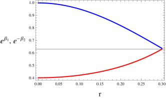
Figure 10: Plots of $e^{\beta_{1}}$ (red) and $e^{-\beta_{2}}$ (blue) corresponding to Model III.

Figure 10 exhibits a singularity-free, positive and finite behavior of $\beta_{1}$ and $\beta_{2}$, indicating physically acceptable solution. Further, we have $e^{\beta_{1}(0)}=\mathcal{C}$ and $e^{-\beta_{2}(0)}=1$ at $r=0$, and they meet at a single point at $r=0.3$. The compactness can now be calculated at the boundary, since we have

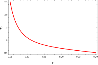
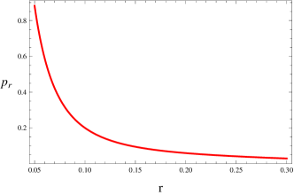
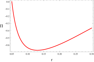
Figure 11: Plots of energy density, radial/tangential pressures and anisotropy corresponding to Model III.

$$e^{\beta_{1}(0.3)}=e^{-\beta_{2}(0.3)}\approx 0.63=1-\frac{2\mathcal{\bar{M}}}{\mathcal{R}}+\frac{\mathcal{\bar{S}}^{2}}{\mathcal{R}^{2}},$$

which gives

$$\frac{2\mathcal{\bar{M}}}{\mathcal{R}}-\frac{\mathcal{\bar{S}}^{2}}{\mathcal{R}^{2}}\approx 0.37<\frac{8}{9}.$$ (50)

Figure 11 indicates acceptable nature of physical variables as they are maximum and positive at the center and then decrease outwards. Here, $p_{t}>p_{r}$ is observed outwards leading to the negative anisotropy (lower right plot). The energy bounds are demonstrated in Figure 12 which are satisfied, therefore, the developed model is viable and contains ordinary matter. Figure 13 (left) manifests the interior redshift that decrease with $r$ and obtain the value at the boundary as $Z(0.3)\approx 1.76<Z_{\mathcal{R}}$. The cracking condition in this case takes negative values only for small radius and then becomes positive (right plot). Hence, our developed solution corresponding to the constraints (34) and (48) is not stable dissimilar to the uncharged case [40].

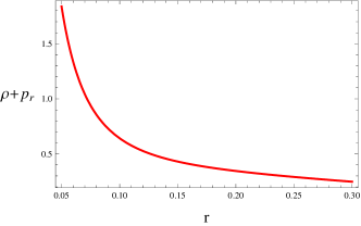
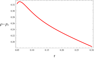
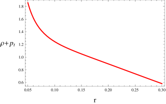
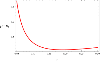
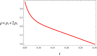
Figure 12: Plots of energy conditions corresponding to Model III.

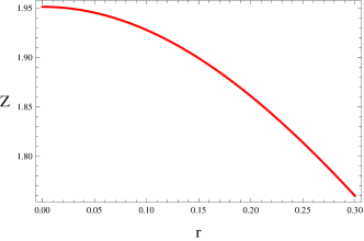
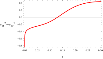
Figure 13: Plots of redshift and cracking condition corresponding to Model III.

6 Conclusions

The purpose of this article is to formulate some different solutions to the Einstein field equations in the presence of an electromagnetic field. For this purpose, we have assumed a static spherically symmetric interior geometry and determined the Einstein-Maxwell field equations as well as the hydrostatic equilibrium condition. We have also expressed mass of the sphere in terms of energy density and charge. The Reissner-Nordström metric has then been taken as an exterior geometry to calculate matching conditions at the spherical boundary. Further, we have split the curvature tensor orthogonally and obtained four distinct scalars associated with several physical parameters. We have observed that a factor $\mathcal{Y}_{TF}$ involved density inhomogeneity, anisotropy and charge, thus adopted it as the complexity factor for the considered matter setup according to the Herrera’s suggested definition [25].

Since the field equations (8)-(10) contain five unknowns, i.e., three matter variables and two metric potentials, we have considered some constraints to make the system solvable. The first of them has been taken as the complexity-free condition given in Eq.(34). Moreover, we have chosen three constraints ($p_{r}=0$, a polytropic and a non-local equation of state, respectively) as the second condition, leading to distinct solutions. The solutions for $\beta_{1}$ and $\beta_{2}$ have been calculated through numerically integrating the corresponding equations in each case along with some initial conditions. We have then presented some physical conditions whose fulfilment leads to realistic stellar models. The matter sector (energy density and pressure) corresponding to each solution has shown accepted behavior (maximum at $r=0$ and decreasing outward). The compactness and surface redshift have also been noticed to be less than their upper limits. All the solutions have met viability criterion as the energy conditions are satisfied. The cracking condition has been fulfilled only by the solutions corresponding to $p_{r}=0$ and a polytropic equation of state, however, it has taken positive values for the case of third model leading to instability of that solution. It is mentioned here that our resulting solutions corresponding to second and third models are not consistent with [40].

Data Availability: No data was used for the research described in this paper.

References

- [1] Herrera, L. and Santos, N.O.: Phys. Rep. 286(1997)53.
- [2] Ovalle, J.: Phys. Rev. D 95(2017)104019.
- [3] Ovalle, J., Casadio, R., da Rocha, R. and Sotomayor, A.: Eur. Phys. J. C 78(2018)122.
- [4] Herrera, L.: Phys. Rev. D 101(2020)104024.
- [5] Herrera, L., Ospino, J. and Di Prisco., A.: Phys. Rev. D 77(2008)027502.
- [6] Abellán, G., Bargueño, P., Contreras, E. and Fuenmayor, E.: Int. J. Mod. Phys. D 29(2020)2050082.
- [7] Chandrasekhar, S.: Mon. Not. R. Astron. Soc. 93(1933)390.
- [8] Liu, F.K.: Mon. Not. R. Astron. Soc. 281(1996)1197.
- [9] Abellán, G., Fuenmayor, E. and Herrera, L.: Phys. Dark Universe 28(2020)100549.
- [10] Tooper, R.F.: Astrophys. J. 140(1964)434.
- [11] Bludman, S.A.: Astrophys. J. 183(1973)637.
- [12] Herrera, L. and Barreto, W.: Phys. Rev. D 88(2013)084022.
- [13] Herrera, L., Di Prisco, A., Barreto, W. and Ospino, J.: Gen. Relativ. Gravit. 46(2014)1827.
- [14] Abellán, G., Fuenmayor, E., Contreras, E. and Herrera, L.: Phys. Dark Universe 30(2020)100632.
- [15] Karmarkar, K.R.: In Proceedings of the Indian Academy of Sciences-Section A 27(1948)56.
- [16] Singh, K.N., Maurya, S.K., Rahaman, F. and Tello-Ortiz, F.: Eur. Phys. J. C 79(2019)381.
- [17] Ospino, J. and Núñez, L.A.: Eur. Phys. J. C 80(2020)166.
- [18] Ramos, A., Arias, C., Fuenmayor, E., and Contreras, E.: Eur. Phys. J. C 81(2021)203.
- [19] Sharif, M. and Naseer, T.: Phys. Scr. 97(2022)055004.
- [20] Sharif, M. and Naseer, T.: Phys. Scr. 97(2022)125016.
- [21] Herrera, L., Di Prisco, A., Ospino, J. and Fuenmayor, E.: J. Math. Phys. 42(2001)2129.
- [22] López-Ruiz, R., Mancini, H.L. and Calbet, X.: Phys. Lett. A 209(1995)321.
- [23] Calbet, X. and López-Ruiz, R.: Phys. Rev. E 63(2001)066116.
- [24] Panos, C.P. Nikolaidis, N.S., Chatzisavvas, K.C. and Tsouros, C.C.: Phys. Lett. A 373(2009)2343.
- [25] Herrera, L.: Phys. Rev. D 97(2018)044010.
- [26] Bel, L.: in Ann. Inst. Henri Poincaré 17(1961)37.
- [27] Herrera, L., Ospino, J., Di Prisco, A., Fuenmayor, E. and Troconis, O.: Phys. Rev. D 79(2009)064025.
- [28] Herrera, L., Di Prisco, A. and Ospino, J.: Phys. Rev. D 98(2018)104059; Phys. Rev. D 99(2019)044049.
- [29] Sharif, M. and Naseer, T.: Chin. J. Phys. 77(2022)2655; Eur. Phys. J. Plus 137(2022)947; ibid. 137(2022)1304; Class. Quantum Grav. 40(2023)035009.
- [30] Pant, N., Mehta, R.N. and Pant, M.: Astrophys. Space Sci. 332(2011)473.
- [31] Gupta, Y.K. and Maurya, S.K.: Astrophys. Space Sci. 332(2011)155
- [32] Pant, N.: Astrophys. Space Sci. 331(2011)633.
- [33] Sharif, M. and Azam, M.: Gen. Relativ. Gravit. 44(2012)1181.
- [34] Sharif, M. and Butt, I.I.: Eur. Phys. J. C 78(2018)688.
- [35] Sharif, M. and Naseer, T.: Chin. J. Phys. 73(2021)179; Fortschr. Phys. 71(2022)2200147; Indian J. Phys. 96(2022)4373.
- [36] Sunzu, J.M., Maharaj, S.D. and Ray, S.: Astrophys. Space Sci. 352(2014)719.
- [37] Murad, M.H.: Astrophys. Space Sci. 20(2016)361.
- [38] Sharif, M. and Sadiq, S.: Eur. Phys. J. C 78(2018)410.
- [39] Sharif, M. and Ama-Tul-Mughani, Q.: Chin. J. Phys. 65(2020)207.
- [40] Arias, C., Contreras, E., Fuenmayor, E. and Ramos, A.: Ann. Phys. 436(2022)168671.
- [41] Tolman, R.C.: Phys. Rev. 35(1930)875.
- [42] Delgaty, M.S.R. and Lake, K.: Comput. Phys. Commun. 115(1998)395.
- [43] Ivanov, B.V.: Eur. Phys. J. C 77(2017)738.
- [44] Giuliani, A. and Rothman, T.: Gen. Relativ. Gravit. 40(2008)1427.
- [45] Naresh, D.: J. Cosmol. Astropart. Phys. 04(2020)035.
- [46] Buchdahl, H.A.: Phys. Rev. 116(1959)1027.
- [47] Herrera, L.: Phys. Lett. A 165(1992)206.
- [48] Abreu, H., Hernández, H. and Núñez, L.A.: Class. Quantum Grav. 24(2007)4631.
- [49] de Felice, F., Yu, Y.Q. and Fang, J.: Mon. Not. R. Astron. Soc. 277(1995)L17.
- [50] Florides, P.S.: Proc. R. Soc. Lond. A Math. Phys. Sci. 337(1974)529.
- [51] Hernández, H. and Núñez, L.A.: Can. J. Phys. 82(2004)29.