NLTGCR: a class of nonlinear acceleration procedures based on Conjugate Residuals

Abstract

This paper develops a new class of nonlinear acceleration algorithms based on extending conjugate residual-type procedures from linear to nonlinear equations. The main algorithm has strong similarities with Anderson acceleration as well as with inexact Newton methods - depending on which variant is implemented. We prove theoretically and verify experimentally, on a variety of problems from simulation experiments to deep learning applications, that our method is a powerful accelerated iterative algorithm.

65F10, 68W25, 65F08, 90C53

1 Introduction

There has been a surge of interest in recent years in numerical algorithms whose goal is to accelerate iterative schemes for solving the following problem:

(1) $$\text{ Find }x\in\mathbb{R}^{n}\text{ such that }f(x)=0,$$

where $f$ is a continuously differentiable mapping from $\mathbb{R}^{n}$ to $\mathbb{R}^{n}$. This problem can itself originate from unconstrained optimization where we need to minimize a scalar function:

(2) $$\min_{x}\phi(x),$$

in which $\phi:\ \mathbb{R}^{n}\to\mathbb{R}$. In this situation we will be interested in a local minimum which can be found as a zero of the system of equations $f(x)=0$ where $f(x)=\nabla\phi(x)$.

The problem (1) can be formulated as a fixed point problem, where one seeks to find the fixed point of a mapping $g$ from $\mathbb{R}^{n}$ to itself:

(3) $$\text{ Find }x\in\mathbb{R}^{n}\text{ such that }x=g(x).$$

This can be achieved by setting, for example, $g(x)=x+\beta f(x)$ for some nonzero $\beta$. Given a mapping $g$, the related fixed point iteration, i.e., the sequence generated by

(4) $$x_{j+1}=g(x_{j})$$

may converge to the fixed point of (3) and when $g(x)=x+\beta f(x)$ then this limit is clearly a solution to the problem (1). However, fixed-point iterations often converge slowly, or may even diverge. As a result acceleration methods are often invoked to improve their convergence, or to establish it.

A number of such acceleration methods have been proposed in the past. It is important to clarify the terminology and discuss the common distinction between acceleration methods which aim at accelerating the convergence of a fixed point sequence of the form (4), and solvers which aim at finding solutions to (1). Among acceleration techniques are ‘extrapolation-type’ algorithms such as the Reduced-Rank Extrapolation (RRE) [69], the Minimal-Polynomial Extrapolation (MPE) [16], the Modified MPE (MMPE) [39], and the vector $\epsilon$-algorithms [11]. These typically produce a new sequence from the original one by combining them without invoking the mapping $g$ in the process. Another class of methods produce a new sequence by utilizing both the iterates and the mapping $g$. Among these, Anderson Acceleration (AA) [4] has received enormous attention in recent years due to its success in solving a wide range of problems [67, 31, 68, 20, 71, 57, 37, 34, 77, 36]. AA can be seen as an inexpensive alternative to second order methods such as quasi-Newton type techniques. It is often used quite successfully without global convergence strategies such as line search or trust-region techniques. These advantages made the method popular in applications ranging from quantum physics, where they were first developed, to machine learning. We refer readers to [12] for a survey of acceleration methods.

As was stated above, it is clear that one can invoke one of these accelerators for solving (1) by applying it to the fixed point sequence associated with $g(x)=x+\beta f(x)$. AA, and its sibling Pulay mixing [60, 61], were devised precisely in this way. Thus, an accelerator of this type can be viewed as a solver, in the same way that a linear accelerator (e.g., Conjugate Gradient) combined with some basic iteration, such as Richardson, can be viewed as a ‘solver’. This class of techniques does not include the extrapolation-type methods discussed above because they require the computation of $g(x)$ for an arbitrary $x$. In extrapolation methods we have a sequence of vectors, but we do not have access to the function $g$ for evaluating $g(x)$.

We can also ask the question whether or not a given solver can be viewed as an accelerator. If the solver only requires evaluating $f(x)$ for an arbitrary $x$ then clearly we can apply it to find the root of the equation $f(x)\equiv x-g(x)=0$, which requires the computation $g(x)$ given $x$. The related iterative process can be viewed as an acceleration technique for the fixed point mapping $g(x)$. Thus, our definition of an accelerator is broad and it encompasses any method that aims to speed up a fixed point iteration by requiring only function evaluations at each step.

A good representative of this class of methods is Anderson Acceleration (AA). There are three issues with AA, and similar accelerators, which this article aims to address. The first is that for optimization problems, AA does not seem to be amenable to exploiting the symmetry of the Jacobian or Hessian. If we had to solve a linear system with AA, the sequence resulting from the algorithm cannot be written in the form of a short-term recurrence, as is the case with Conjugate Gradient or Conjugate Residual algorithm for example. For nonlinear optimization problems where the Hessian is symmetric, this indicates that AA does not take advantage of symmetry and as such it may become expensive in terms of memory and computational cost. This is especially true in a nonconvex stochastic setting, where a large number of iterates are often needed. This can be an acute problem, particularly in machine learning, where we often encounter practical situations in which the number of parameters is quite large, making it impracical to use a large number of vectors in AA. Although recent literature made efforts to improve the convergence speed of AA [77, 76, 51, 67, 80, 35], they did not attempt to reduce memory cost. One of the goals of this paper is to propose an acceleration technique that exploits symmetry or near symmetry to reduce the computational cost.

A second problem with AA, which is perhaps a result of its simplicity, is that while it shares some similarities with quasi-Newton methods, it does not exploit standard methods that are common in second order methods to improve global convergence characteristics. The inclusion of line search or trust-region methods is necessary if one wishes to solve realistic problems. A secondary goal of this paper is to introduce an AA-like method that implements global convergence strategies borrowed from inexact Newton and quasi-Newton methods.

Finally, one of the issues with AA, and other acceleration methods, is that it uses a crude linear model. Specifically, acceleration methods typically rely on two sets of consecutive vector differences, namely the differences $\Delta f_{i}\equiv f(x_{i+1})-f(x_{i})$ and the associated $\Delta x_{i}\equiv x_{i+1}-x_{i}$. The issue is that their approximate solutions are developed from the relation $\Delta f_{i}\approx J(x_{i})\Delta x_{i}$, where $J(x_{i})$ is the Jacobian at $x_{i}$. This linear approximation is likely to be rather inaccurate, especially when the iterate is far from its limit. It is important to develop techniques that will avoid relying on such rough approximations.

Nonlinear acceleration methods of the type discussed in this paper appeared first in the physics literature where they were needed to accelerate very complex and computationally intensive processes, such as the Self-Consistent Field (SCF) iteration. The best known of these methods was discovered by Anderson [4] in 1965. In the early 1980s, Pulay proposed a similar scheme which he called Direct Inversion on the Iterative Subspace (DIIS) [60, 61]. Both methods were designed specifically for SCF iterations and it turns out that, although formulated differently, AA and DIIS are essentially equivalent, see, e.g.,  [19, 28, 47]. For this reason the method is often referred to as ‘Anderson-Pulay mixing’, where mixing in this context refers to the process by which a new fixed point iterate is mixed with previous ones to accelerate the process. AA was rediscovered again in a different form in a 2000 paper by Oosterlee and Washio [56] who applied their technique to accelerate nonlinear multigrid iterations.

The link between nonlinear acceleration methods such as AA and secant-type methods was first unraveled by Eyert [27] when he compared AA with a multi-secant method proposed by Vanderbilt and Louie more than a decade earlier [73]. The article [62] explored this idea further and expanded on it by proposing two classes of multi-secant methods. Thereafter, AA started to be studied and utilized by researchers outside the field of physics, see, e.g.,  [21, 75, 72, 50, 7, 58, 26] among many others.

The primary contribution of the present paper is to take another look at this class of methods and develop a technique that is derived by a careful extension of a linear iterative method to nonlinear systems. The paper is motivated primarily by a desire to overcome the three weaknesses of AA mentioned earlier.

2 Background: Inexact Newton, quasi-Newton, and Anderson acceleration

The goal of this section is to clarify key features of the method proposed in this paper in order to establish links with known methods. Many of the approaches developed for solving (1) are rooted in Newton’s method which exploits the local linear model:

(5) $$f(x+\Delta x)\approx f(x)+J(x)\Delta x,$$

where $J(x)$ is the Jacobian matrix at $x$.

Notation

We will often refer to an evolving set of columns where the most recent vectors from a sequence are retained. In this situation, we found it convenient to use the following convention. For a given $m\geq 0$ we set:

(6) $$j_{m}=\max\{0,j-m+1\}\quad m_{j}=\min\{m,j+1\}\equiv j-j_{m}+1.$$

2.1 Inexact Newton methods

Newton’s method determines $\Delta x_{j}=x_{j+1}-x_{j}$ at step $j$, to make the right-hand side on (5) equal to zero when $x=x_{j}$, which is achieved by solving the Newton linear system $J(x_{j})\delta+f(x_{j})=0.$ Inexact Newton methods, e.g., [41, 22, 13] among many references, compute a sequence of iterates in which the above Newton systems are solved approximately, often by an iterative method. Given an initial guess $x_{0}$, the iteration proceeds as follows:

(7) Solve $$J(x_{j})\delta_{j} \approx-f(x_{j})$$

(8) Set $$x_{j+1} =x_{j}+\delta_{j}$$

Note that the right-hand side of the Newton system is $-f(x_{j})$ and this is also the residual for the linear system when $\delta_{j}=0$. Therefore, in later sections we will define the residual vector $r_{j}$ to be $r_{j}\equiv-f(x_{j})$.

The technique for solving the local system (7) is not specified. Suppose that we invoke a Krylov subspace method for solving (7). If we set $J\equiv J(x_{j})$ then the method, will usually generate an approximate solution that can be written in the form

(9) $$\delta_{j}=V_{j}y_{j},$$

where $V_{j}$ is an orthonormal basis of the Krylov subspace

(10) $$K_{j}=\mbox{Span}\{r_{j},Jr_{j},\cdots,J^{m-1}r_{j}\}.$$

The vector $y_{j}$ represents the expression of the solution in the basis $V_{j}$. For example, if GMRES or, equivalently Generalized Conjugate Residual (GCR) [23], is used, then $y_{j}$ becomes $y_{j}=(JV_{j})^{\dagger}(-f(x_{j}))$. In essence the inverse Jacobian is approximated by the rank $m$ matrix:

$$B_{j,GMRES}=V_{j}(JV_{j})^{\dagger}.$$

In inexact Newton methods the approximations just defined are valid only for the $j$-th step, i.e., once the solution is updated, they are discarded and the process will essentially compute a new Krylov subspace and related approximate Jacobian at point $x_{j+1}$. This ‘lack of memory’ can be an impediment to performance. In contrast, quasi-Newton methods will compute approximate Jacobians or their inverses by a process that is continuously being updated, using the most recent iterate for this update.

2.2 Quasi-Newton methods

Standard quasi-Newton methods build a local approximation $J_{j}$ to the Jacobian $J(x_{j})$ progressively by using previous iterates. These methods require the relation (5) to be satisfied by the updated $J_{j+1}$ which is built at step $j$. This means that the following secant condition, is imposed:

(11) $$J_{j+1}\Delta x_{j}=\Delta f_{j},$$

where $\Delta f_{j}:=f(x_{j+1})-f(x_{j})$. The following no-change condition is also imposed:

(12) $$J_{j+1}q=J_{j}q,\quad\forall q\quad\mbox{such that}\quad q^{T}\Delta x_{j}=0.$$

In other words, there should be no new information from $J_{j}$ to $J_{j+1}$ along any direction $q$ orthogonal to $\Delta x_{j}$. Broyden showed that there is a unique matrix $J_{j+1}$ that satisfies both conditions (11) and (12) and it can be obtained by the update formula:

(13) $$J_{j+1}=J_{j}+(\Delta f_{j}-J_{j}\Delta x_{j})\frac{\Delta x_{j}^{T}}{\Delta x_{j}^{T}\Delta x_{j}}.$$

Broyden’s second method approximates the inverse Jacobian directly instead of the Jacobian itself. If $G_{j}$ denotes this approximate inverse Jacobian at the $j$-th iteration, then the secant condition (11) becomes:

(14) $$G_{j+1}\Delta f_{j}=\Delta x_{j}.$$

By minimizing $E(G_{j+1})=\|G_{j+1}-G_{j}\|_{F}^{2}$ with respect to $G_{j+1}$ subject to (14), one finds this update formula for the inverse Jacobian:

(15) $$G_{j+1}=G_{j}+(\Delta x_{j}-G_{j}\Delta f_{j})\frac{\Delta f_{j}^{T}}{\Delta f_{j}^{T}\Delta f_{j}},$$

which is also the only update satisfying both the secant condition (14) and the no-change condition for the inverse Jacobian:

(16) $$(G_{j+1}-G_{j})q=0,\quad\forall\ q\perp\Delta f_{j}.$$

We will revisit secant-type methods again when we discuss AA in the next section. AA can be viewed from the angle of multi-secant methods, i.e., block forms of the secant methods just discussed, in which we impose a secant condition on a whole set of vectors $\Delta x_{i},\Delta f_{i}$ at the same time.

2.3 General nonlinear acceleration and Anderson’s method

Acceleration methods, such as AA, take a different viewpoint altogether. Their goal is to accelerate a given fixed point iteration of the form (4). Thus, AA starts with an initial $x_{0}$ and sets $x_{1}=g(x_{0})=x_{0}+\beta f_{0}$, where $\beta>0$ is a parameter. At step $j>m$ we define $X_{j}=[x_{j-m},\ldots,x_{j-1}],$ and $F_{j}=[f_{j-m},\ldots,f_{j-1}]$ along with the differences:

(17) $$\mathcal{X}_{j}=[\Delta x_{j-m}\;\cdots\;\Delta x_{j-1}]\in\mathbb{R}^{n\times m},\qquad\mathcal{F}_{j}=[\Delta f_{j-m}\;\cdots\;\Delta f_{j-1}]\in\mathbb{R}^{n\times m}.$$

We then define the next AA iterate as follows:

(18) $$x_{j+1} =x_{j}+\beta f_{j}-(\mathcal{X}_{j}+\beta\mathcal{F}_{j})\ \theta^{({j})}\quad\mbox{where:}$$

(19) $$\theta^{({j})} =\text{argmin}_{\theta\in\mathbb{R}^{m}}\|f_{j}-\mathcal{F}_{j}\theta\|_{2}.$$

Note that $x_{j+1}$ can be expressed with the help of intermediate vectors:

(20) $$\bar{x}_{j}=x_{j}-\mathcal{X}_{j}\ \theta^{({j})},\quad\bar{f}_{j}=f_{j}-\mathcal{F}_{j}\ \theta^{({j})},\quad x_{j+1}=\bar{x}_{j}+\beta\bar{f}_{j}.$$

There is an underlying quasi-Newton second order method aspect to the procedure. In Broyden-type methods, Newton’s iteration: $x_{j+1}=x_{j}-J(x_{j})^{-1}f_{j}$ is replaced with $x_{j+1}=x_{j}-G_{j}f_{j}$ where $G_{j}$ approximates the inverse of the Jacobian $J(x_{j})$ at $x_{j}$ by the update formula $G_{j+1}=G_{j}+(\Delta x_{j}-G_{j}\Delta f_{j})v_{j}^{T}$ in which $v_{j}$ is defined in different ways see [62] for details. AA belongs to the class of multi-secant methods. Indeed, the approximation (18) can be written as:

(21) $$x_{j+1}=x_{j}-[-\beta I+(\mathcal{X}_{j}+\beta\mathcal{F}_{j})(\mathcal{F}_{j}^{T}\mathcal{F}_{j})^{-1}\mathcal{F}_{j}^{T}]f_{j}\equiv x_{j}-G_{j}f_{j}.$$

Thus, $G_{j}$ can be seen as an update to the (approximate) inverse Jacobian $G_{j-m}=-\beta I$ by the formula:

(22) $$G_{j}=G_{j-m}+(\mathcal{X}_{j}-G_{j-m}\mathcal{F}_{j})(\mathcal{F}_{j}^{T}\mathcal{F}_{j})^{-1}\mathcal{F}_{j}^{T}.$$

It can be shown that the approximate inverse Jacobian $G_{j}$ is the result of minimizing $\|G_{j}+\beta I\|_{F}$ under the multi-secant condition of type II

(23) $$G_{j}\mathcal{F}_{j}=\mathcal{X}_{j}.$$

This link between AA and Broyden multi-secant type updates was first unraveled by Eyert [27] and expanded upon in [62]. Thus, the method is in essence what we might call a ‘block version’ of Broyden’s second update method, whereby a rank $m$, instead of rank $1$, update is applied at each step.

2.4 The issue of symmetry

Consider again the specific case where the nonlinear function $f(x)$ is the gradient of some scalar function $\phi(x)$ to be minimized, i.e., $f(x)=\nabla\phi(x)$. In this situation the Jacobian of $f$ becomes $\nabla^{2}\phi$ the Hessian of $\phi$, and therefore it is symmetric. Approximate Jacobians that are implicitly or explicitly extracted in the algorithm, will be symmetric or nearly symmetric. Therefore this raises the possibility of developing accelerators that take advantage of symmetry or near-symmetry. One way to achieve this is to extend linear solvers that take advantage of symmetry to the nonlinear context. This was one of the primary initial motivations for this work.

We saw earlier that AA is a multi-secant version of a Broyden type II method where the approximate inverse Jacobian is updated by formula (22). An obvious observation here is that the symmetry of the Jacobian can not be exploited in any way in this formula. This has been considered in the literature (very) recently, see for example, [8, 66, 9]. In a 1983 report, Schnabel [65] showed that the matrix $G_{j}$ obtained by a multi-secant method that satisfies the secant condition (23) is symmetric iff the matrix $\mathcal{X}_{j}^{T}\mathcal{F}_{j}$ is symmetric. It is possible to explicitly force symmetry by employing generalizations of the symmetric versions of Broyden-type methods. Thus, the authors of [8, 9] recently developed a multi-secant version of the Powell Symmetric Broyden (PSB) update due to Powell [59] while the article [66] proposed a symmetric multi-secant method based on the popular Broyden-Fletcher-Goldfarb-Shanno (BFGS) approach as well as the Davidon-Fletcher-Powell (DFP) update. However, there are a number of issues with the symmetric versions of multi-secant updates some of which are discussed in [66].

3 Nonlinear Truncated Generalized Conjugate Residual (nlTGCR) algorithm

For understanding the conjugate residual-based methods in the nonlinear case, it is important to first provide some background for linear systems. A large class of Krylov subspace methods for solving nonsymmetric linear systems have been developed in the past four decades. The reader is referred to the recent volume by Meurant and Tebbens [53] which contains a rather exhaustive and detailed coverage of these methods. The main aim of the techniques proposed in this article is to adapt the residual-minimizing subclass of Krylov methods for linear systems to the nonlinear case. The guiding principle in this adaption is that we would like it to also approximately minimize the nonlinear residuals. This is in contrast with inexact Newton methods where the goal is to roughly solve the linear systems that arise in Newton’s method as a way to provide a good search direction.

3.1 The linear case: Generalized Conjugate Residual (GCR) Algorithm

We first consider solving a linear system of the form:

(24) $$Ax=b.$$

A number of iterative methods developed in the 1980s aimed at minimizing the norm of the residual $r=b-Ax$ of a new iterate that lies in a Krylov subspace, see [53] for a detailed account. Among these, we focus on the Generalized Conjugate Residual (GCR) algorithm [23] for solving (24) which is sketched in Algorithm 1.

Algorithm 1 GCR

1:Input: Matrix $A$, RHS $b$, initial $x_{0}$.

2:Set $p_{0}:=r_{0}\equiv b-Ax_{0}$.

3:for $j=0,1,2,\cdots,$ until convergence do

4:     $\alpha_{j}:=\langle r_{j},Ap_{j}\rangle/\langle Ap_{j},Ap_{j}\rangle$

5:     $x_{j+1}:=x_{j}+\alpha_{j}p_{j}$

6:     $r_{j+1}:=r_{j}-\alpha_{j}Ap_{j}$

7:     $p_{j+1}:=r_{j+1}-\sum_{i=0}^{j}\beta_{ij}p_{i}$  where  $\beta_{ij}:=\langle Ar_{j+1},Ap_{i}\rangle/\langle Ap_{i},Ap_{i}\rangle$

8:end for

The main point of the algorithm is to build a sequence of search directions $p_{i}$, $i=0:j$ at step $j$ so that the vectors $Ap_{i}$ are orthogonal. This is done in Line 7. With this we know that the iterate as defined by Lines 4-5 is optimal in the sense that it yields the smallest residual norm among solution vectors selected from the Krylov subspace $x_{0}+\mbox{\mbox{Span}}\{p_{0},\ldots,p_{k}\}$ – see [63, pp 195-196]. The GCR algorithm is mathematically equivalent to GMRES [64], and to some of the forms of other methods developed earlier, e.g., ORTHOMIN [74], ORTHODIR [40], and Axelsson’s CGLS method [6].

Next we will discuss a truncated version of GCR in which the $Ap_{i}$’s are only orthogonal to the $m$ previous ones instead of all of them. This algorithm was first introduced by Vinsome as early as in 1976 and was named ‘ORTHOMIN’ [74]. We will just refer to it as the truncated version of GCR or TGCR(m). In a practical implementation, we need to keep a set of $m$ vectors at step $j$ for the $p_{i}$’s and another set for the vectors $v_{i}=Ap_{i}$. In addition, we replace the classical Gram-Schmidt of Line 7 of Algorithm 1 by the modified form of Gram-Schmidt: the vector $Ar_{j+1}$ initially set to a vector $v$ which is orthogonalized against the successive $Ap_{i}$’s. Thus, Line 7 of Algorithm 1 becomes:

7a.	$p:=r_{j+1}$; $v:=Ap$; and $j_{m}:=\max(0,j-m+1)$
7b.	for  $i=j_{m}:j$
7c.		$\beta_{ij}:=\langle v,Ap_{i}\rangle$
7d.		$p:=p-\beta_{ij}p_{i}$;	$v:=v-\beta_{ij}v_{i}$;
7e.	end for
7f.	$p_{j+1}:=p/\|v\|$ ;		$v_{j+1}:=v/\|v\|$ ;

We refer to the Algorithm obtained from Algorithm 1 where Line 7 is replaced by Lines (7a–7f) above as the Truncated GCR (TGCR(m)) algorithm. This algorithm is a slight variant of the original ORTHOMIN introduced in [74] and analyzed in [23]. It produces a system of vectors $V_{j+1}=[v_{j_{m}},v_{j_{m}+1},\ldots,v_{j},v_{j+1}]$ that is orthonormal. When $j\geq m$, $V_{j+1}$ consists of a ‘window’ of $m+1$ vectors. TGCR(m) approximately minimizes the quadratic form $\phi_{q}(x)\equiv\frac{1}{2}\|b-Ax\|_{2}^{2}$ in a certain Krylov subspace. With $m=\infty$ we obtain the non-restarted GCR method - which is equivalent to the non-restarted GMRES [64].

A few properties of the vectors generated in TGCR(m) have been analyzed in  [23, Th. 4.1] which also discussed the convergence of the algorithm when $A$ is positive definite, i.e., when $A+A^{T}$ is symmetric positive definite. When $A$ is symmetric a number of simplifications take place in Algorithm  1. In this situation, all the $\beta_{ij}$’s except $\beta_{jj}$ vanish. The resulting simplified algorithm yields the standard Conjugate Residual (CR) algorithm which dates back to Stiefel [70], see [64, Section 6.8] for details.

3.2 The nonlinear extension: nonlinear TGCR (nlTGCR) algorithm

We now return to the nonlinear problem and ask the question: how can we generalize the algorithms for linear systems of Section 3.1 for solving nonlinear equations? We should begin by stating what are the desired features of this extension. First we would like the algorithms to fall back to TGCR when the problem is linear. Second, we would like a method that can be adapted in such a way as to yield the inexact Newton viewpoint when desired or a multi-secant (AA-like) approach when desired. Third, we would like a method that exploits a more accurate linear model than either Newton or a quasi-Newton approach - possibly at the cost of a few extra function evaluations. Finally, we would like the algorithm to be easily adaptable to the very common context in which the function $f$ is ‘fuzzy’ as is the case when dealing with stochastic methods.

In our model we assume that at step $j$ we have a set of (at most) $m$ current ‘search’ directions $\{p_{i}\}$ for $j_{m}\leq i\leq j$ gathered as columns of a matrix $P_{j}$, where we recall the notation $j_{m}\equiv\max\{0,j-m+1\}$. Along with $p_{i}$’s, we also have a matrix denoted by $V_{j}$, such that

(25) $$P_{j}=[p_{j_{m}},p_{j_{m}+1},\cdots,p_{j}],\qquad V_{j}=[v_{j_{m}},v_{j_{m}+1},\cdots,v_{j}].$$

Note that this pair of matrices plays the same role as does the pair $\mathcal{X}_{j},\ \mathcal{F}_{j}$ defined in (17) for Anderson acceleration. We then write the linear model used locally as

(26) $$f(x_{j}+P_{j}y)\approx f(x_{j})+V_{j}y.$$

While this is again somewhat similar to what was done for Anderson acceleration, we note a very important distinction that may have a significant effect on performance: In Anderson acceleration the linear model is simply based on the relation $f(x_{j}-\mathcal{X}_{j}\theta)\approx f(x_{j})-\mathcal{F}_{j}\theta$ whereas nlTGCR evaluates explicitly the action of $J(x_{i})$ on some vector. This evaluation can be quite accurate if desired. In contrast, the relation $f(x_{j}-\mathcal{X}_{j}\theta)\approx f(x_{j})-\mathcal{F}_{j}\theta$ can be quite rough, especially at the beginning of the process where the vectors $\Delta x_{j}$ and $\Delta f_{j}$ are usually not small.

The projection method will minimize the norm $\|f(x_{j})+V_{j}y\|_{2}$. This is achieved by determining $y$ in such a way that

(27) $$f(x_{j})+V_{j}y\perp\mbox{Span}\{V_{j}\}\ \rightarrow\ (V_{j})^{T}[f(x_{j})+V_{j}y]=0\ \rightarrow\ y=V_{j}^{T}r_{j}$$

where it is assumed the $v_{i}$’s are orthonormal.

Instead of (7–8) of the inexact Newton approach we now have an iteration of the form

(28) Find $$y_{j} =\mbox{argmin}_{y}\|f(x_{j})+V_{j}y\|_{2}$$

(29) Set $$x_{j+1} =x_{j}+P_{j}y_{j}$$

A major distinction between this approach and the standard inexact Newton is that the latter exploits approximations to the Jacobian around one point in order to build the next iterate. The iterates generated by the iterative process can be viewed as intermediate points but they rely on a Jacobian $J(x_{0})$ calculated at the initial approximation $x_{0}$. We will revisit the inexact Newton viewpoint in a later section.

The idea of the nonlinear version of the truncated GCR method is to exploit the directions that are produced by the TGCR algorithm. Note here is that there is a decoupling between the update from the current iterate (Lines (4-5) of GCR/TGCR) to a new one and the construction of the $p_{i}$’s in TGCR (Lines (7a-7f) of TGCR). In essence, the first part just builds a new approximation given a new ‘search’ subspace - while the second adds a new direction to this evolving subspace. This distinction will help us generalize our approach to cases where the objective function or the Jacobian varies as the iteration proceeds.

Algorithm 2 nlTGCR(m)

1:Input: $f(x)$, initial $x_{0}$.

2:Set $r_{0}:=-f(x_{0})$.

3:Compute $v:=J(x_{0})r_{0}$;  (Use Frechet)

4:$v_{0}:=v/\|v\|$, $p_{0}:=r_{0}/\|v\|_{2}$;

5:for $j=0,1,2,\cdots,$  do

6:     $y_{j}:=V_{j}^{T}r_{j}$

7:     $x_{j+1}:=x_{j}+P_{j}y_{j}$

8:     $r_{j+1}:=-f(x_{j+1})$

9:     Set: $p:=r_{j+1}$; and $j_{m}:=\max(0,j-m+1)$

10:     Compute $v=J(x_{j+1})p$ (Use Frechet)

11:     for $i=j_{m}:j$ do

12:         $\beta_{ij}:=\langle v,v_{i}\rangle$

13:         $p:=p-\beta_{ij}p_{i}$

14:         $v:=v-\beta_{ij}v_{i}$

15:     end for

16:     $p_{j+1}:=p/\|v\|_{2}$ ;   $v_{j+1}:=v/\|v\|_{2}$ ;

17:end for

We now derive our general algorithm from which a few variants will follow. The algorithm is an extension of the TGCR(m) algorithm discussed above – with a few needed changes that reflect the nonlinearity of the problem. The first change is that any residual is now to be replaced by the negative of $f(x)$ so $r_{0}$ becomes $r_{0}=-f(x_{0})$ and Line 6 of GCR/TGCR(m) must be replaced by $r_{j+1}=-f(x_{j+1})$. In addition, the matrix $A$ in the products $Ar_{0}$ and $Ap$ invoked in Line 2 and Line 7.a respectively, is the Jacobian of $f$ at the most recent iterate. The most important change is in Lines (4-5) of Algorithm 1 where according to the above discussion the scalar $\alpha_{j}$ is to be replaced by the vector $y_{j}$ that minimized $\|f(x_{j})+V_{j}y\|_{2}$ over $y$. The reason for this was explained above.

The resulting nlTGCR(m) algorithm is shown in Algorithm 2. It requires two function evaluations per step : one in Line 8 and the other in Line 10. In the situation when computing the Jacobian is inexpensive, then one can compute $Jp$ in Line 10 as a matrix-vector product. Clearly, the system $[v_{j_{m}},v_{j_{m}+1},\cdots,v_{j+1}]$ is orthonormal.

4 Theoretical results

This section discusses connections of nlTGCR(m) algorithm with inexact and quasi-Newton methods and analyzes its convergence.

4.1 Linearized update version and the connections to inexact Newton methods

We first consider a variant of the algorithm which we call the “linearized update version”. We will show that this version is equivalent to inexact Newton methods in which the system is approximately solved with TGCR(m). Two changes are made to Algorithm 2 to obtain this linearized update version. First, in Line 8 we update the residual by using the linear model, namely, we replace Line 8 by:

8a:	$r_{j+1}=r_{j}-V_{j}y_{j}$

The second change is that the Jacobian is not updated in Line 10, i.e., $J(x_{j+1})$ in Line 10 is kept constant and equal to $J(x_{0})$. In other words $v$ is computed as

10a:	$v=J(x_{0})p$

The algorithm is stopped when the residual norm $r_{j+1}$ is small enough or the number of steps is exceeded. In addition, we consider the algorithm merely as a means of providing a search direction as is often done with inexact Newton methods. In other words the direction $d=x_{last}-x_{0}$ is provided to another function which will use it in an iterative procedure that includes a line search technique at $x_{0}$.

It is easy to see that one iteration defined as a sweep using $j$ substeps of this linear update version is nothing but an inexact Newton method in which the system (7) (with $j=0$) is approximately solved with the TGCR(m) algorithm. Indeed, in this situation the two main loops, (Lines 3–8 of Algorithm GCR/TGCR(m) and Lines 5-17 of Algorithm 2) are identical. Lines 5-17 of Algorithm 2 perform $k$ steps of the TGCR(m) algorithm to solve the linear systems $f(x_{0})+J(x_{0})Py=0$. Within Algorithm 2 the update is written in a progressive form as $x_{j+1}=x_{j}+\alpha_{j}p_{j}$, note that the right-hand side does not change during the algorithm and is equal to $r_{0}=-f(x_{0})$. In effect the last iterate, $x_{k}$, is updated from $x_{0}$ by adding a vector from the Krylov subspace or equivalently the span of $P_{k}$. As a consequence of this observation, it turns out that $y_{j}$ has only one nonzero component, namely the last one. Indeed, from  [23, Th. 4.1], we see that if we replace $A$ by the Jacobian $J$ at $x_{0}$ then:

$$\langle r_{j+1},Jp_{i}\rangle=0\ \mbox{for}\ i=(j-1)_{m},\cdots,j.$$

It was shown in [13] that under mild conditions, the update to the iterate is a descent direction. In addition, the article describes ‘global convergence strategies’ based on line search and trust-region techniques. If we do not apply a global convergence strategy, then the algorithm may have difficulties to converge.

Inexact Newton methods [22] are often implemented with residual reduction stopping criteria of the form

(30) $$\|f(x_{j})+J(x_{j})\delta_{j}\|_{2}\leq\eta_{j}\|f(x_{j})\|_{2}$$

where $\eta_{j}\in[0,1)$ is called the forcing term. This only means that the iterative procedure that is applied when approximately solving the linear system (7) exits when the relative residual norm falls below $\eta_{j}$. A number of articles established convergence conditions under conditions based on this framework, see, e.g., [22, 13, 14, 24] among others.

Probably the most significant disadvantage of inexact Newton methods is that a large number of function evaluations may be needed to build the Krylov subspace in order to obtain a single iterate, i.e., the next iterate. After this iterate is computed, all the information gathered at this step, e.g., $P_{k},V_{k}$, is discarded. This is to be contrasted with quasi-Newton techniques where the most recent function evaluation contributes to building an updated approximate Jacobian.

4.2 Nonlinear update version

The “linearized update version” of Algorithm 2 discussed above uses a simple linear model to update the residual $r_{j}$ in which the Jacobian is not updated. Next, we consider the “nonlinear update version” as described in Algorithm 2.

Assume a sweep using $j$ substeps of Algorithm 2 has been carried out. Our next result will invoke the linear residual

(31) $$\tilde{r}_{j+1}=r_{j}-V_{j}y_{j},$$

as well as the deviation between the actual residual $r_{j+1}$ and its linear version $\tilde{r}_{j+1}$ at the $(j+1)$-th iteration:

(32) $$z_{j+1}=\tilde{r}_{j+1}-r_{j+1}.$$

We first analyze the magnitude of $z_{j+1}$. Define

(33) $$w_{i}=J(x_{j})p_{i}-v_{i}\ \mbox{for}\ i=j_{m},\cdots,j;\quad\mbox{and}\quad W_{j}=[w_{j_{m}},\cdots,w_{j}].$$

so that,

(34) $$J(x_{j})p_{i}=v_{i}+w_{i}.$$

Note that the algorithm suggests that $J(x_{i})p_{i}\approx v_{i}$ but that equality is not satisfied except in the linear case . We also define:

(35) $$s_{j}=f(x_{j+1})-f(x_{j})-J(x_{j})(x_{j+1}-x_{j}).$$

Recall from the Taylor series expansion $s_{j}$ is a second order term relative to $\|x_{j+1}-x_{j}\|_{2}$. Then we derive the following bound on the norm of $z_{j+1}$ in the next proposition.

Proposition 4.1.

The difference $\tilde{r}_{j+1}-r_{j+1}$ satisfies the relation:

(36) $$\tilde{r}_{j+1}-r_{j+1}=W_{j}y_{j}+s_{j}=W_{j}V_{j}^{T}r_{j}+s_{j},$$

and therefore:

(37) $$\|\tilde{r}_{j+1}-r_{j+1}\|_{2}\leq\|W_{j}\|_{2}\ \|r_{j}\|_{2}+\|s_{j}\|_{2}.$$

Proof 4.2.

We rewrite the difference as:

$$\tilde{r}_{j+1}-r_{j+1} =(-f(x_{j})-V_{j}y_{j})+f(x_{j+1})$$

$$=(f(x_{j+1})-f(x_{j}))-V_{j}y_{j}$$

(38) $$=J(x_{j})P_{j}y_{j}+s_{j}-V_{j}y_{j}$$

Letting $y_{j}=[\eta_{j_{m}},\eta_{j_{m}+1},\cdots]$ we get from (34)

$$J(x_{j})P_{j}y_{j} =\sum\eta_{i}J(x_{j})p_{i}=\sum\eta_{i}[v_{i}+w_{i}]$$

(39) $$=V_{j}y_{j}+W_{j}y_{j}.$$

The proof follows by combining (38) and (39)

The Proposition 4.1 shows that $z_{j+1}$ is a quantity of the second order: when the process is nearing convergence, $\|W_{j}\|_{2}\|r_{j}\|_{2}$ is the product of two first order terms while $s_{j}$ is a second order term according to its definition (35). Furthermore, we can prove the following properties of Algorithm 2.

Proposition 4.3.

The following properties are satisfied by the vectors produced by Algorithm 2:

1. $(\tilde{r}_{j+1},v_{i})=0\quad\mbox{for}\quad j_{m}\leq i\leq j$, i.e., $V_{j}^{T}\tilde{r}_{j+1}=0$;

2. $\|\tilde{r}_{j+1}\|_{2}=\min_{y}\|-f(x_{j})+V_{j}y\|_{2}$;

3. $\langle v_{j+1},\tilde{r}_{j+1}\rangle=\left\langle v_{j+1}\ ,r_{j}\right\rangle$;

4. $y_{j}=V_{j}^{T}r_{j}=\langle v_{j},\tilde{r}_{j}\rangle e_{m_{j}}-V_{j}^{T}z_{j}$ where $e_{m_{j}}=[0,0,\cdots,1]^{T}\in\ \mathbb{R}^{m_{j}}$.

Proof 4.4.

Properties (1) and (2) follow from the definition of the algorithm. For Property (3) first observe that $V_{j}=[v_{j_{m}},v_{j_{m}+1},\cdots,v_{j-1},v_{j}]$ and that $v_{j+1}$ is made orthogonal against the $m_{j}$ vectors $v_{j_{m}}$ to $v_{j}$, so $v_{j+1}^{T}V_{j}=0$ and

$$v_{j+1}^{T}\tilde{r}_{j+1}=v_{j+1}^{T}[r_{j}-V_{j}y_{j}]\ =\ v_{j+1}^{T}r_{j}.$$

It is convenient to prove Property (4) for the index $j+1$ instead of $j$. We write: $V_{j+1}^{T}r_{j+1}=V_{j+1}^{T}[\tilde{r}_{j+1}-z_{j+1}]$ where $z_{j+1}$ was defined in Equation (32). Recalling Properties (1) and (3), we have that $\langle\tilde{r}_{j+1},v_{i}\rangle=0$ for $j_{m}\leq i\leq j$ - so there is only one nonzero term in the product $V_{j+1}^{T}\tilde{r}_{j+1}$, namely $v_{j+1}^{T}\tilde{r}_{j+1}$. This gives the results after adjusting for the change of index.

Property (4) in Proposition 4.3 indicates that when $z_{j}$ is small, as when the model is close to being linear or when it is nearing convergence, then $y_{j}$ will have small components everywhere except for the last component. As a result it is also possible to consider a slight variant of the algorithm in which $y_{j}$ is truncated so as to contain only its last entry. We will discuss this variant in detail in Section 4.4.

4.3 Connections to quasi-Newton and multi-secant methods

In this section, we show that nlTGCR(m) can be viewed from the alternative angle of a quasi-Newton/multi-secant approach. In this viewpoint, the inverse of the Jacobian is approximated progressively. Because it is the inverse Jacobian that is approximated, the method is akin to Broyden’s second update method.

First observe that in nlTGCR the update at step $j$ takes the form:

$$x_{j+1}=x_{j}+P_{j}V_{j}^{T}r_{j}=x_{j}+P_{j}V_{j}^{T}(-f(x_{j})).$$

Thus, we are in effect using a secant-type method. The approximate inverse Jacobian at step $j$, denoted by $G_{j+1}$ for consistency with common notation, is:

(40) $$G_{j+1}=P_{j}V_{j}^{T}.$$

If we apply this to $v_{i}$ we get $G_{j+1}v_{i}=P_{j}V_{j}^{T}v_{i}=p_{i}\quad\mbox{for}\quad j_{m}\leq i\leq j.$ It therefore satisfies the secant equation

(41) $$G_{j+1}v_{i}=p_{i}\quad\mbox{for}\quad j_{m}\leq i\leq j,$$

which is a version of (14) used in Broyden’s second update method. Here, $p_{i}$ plays the role of $\Delta x_{j}$ and $v_{i}$ plays the role of $\Delta f_{j}$. In addition, the update $G_{j+1}$ satisfies the ‘no-change’ condition:

(42) $$G_{j+1}q=0\quad\forall q\perp v_{i}\quad\mbox{for}\quad j_{m}\leq i\leq j.$$

The usual no-change condition for secant methods is of the form $(G_{j+1}-G_{j-m})q=0$ for $q\perp\Delta f_{j}$ which in our case would be $(G_{j+1}-G_{j-m})q=0$ for $q\perp\ v_{i}\quad\mbox{for}\quad j_{m}\leq i\leq j$. One can therefore consider that we are updating $G_{j-m}\equiv 0$.

Thus, consider the optimization problem

(43) $$\min\{\|G\|_{F}\ \text{subject to: }\quad GV_{j}=P_{j}\}$$

which will yield the matrix of smallest F-norm satisfying the condition (41). Not surprisingly this matrix is just $G_{j+1}$.

Proposition 4.5.

The unique minimizer of Problem (43) is the matrix $G_{j+1}$ given by (40).

Proof 4.6.

The index $j$ is dropped from this proof. Exploiting orthogonal projectors we write $G$ as follows: $G=GVV^{T}+G(I-VV^{T})=PV^{T}+G(I-VV^{T})$ and observe that

$$\|G\|_{F}^{2} =\text{tr}\left([PV^{T}+G(I-VV^{T})][VP^{T}+(I-VV^{T})G^{T}]\right)$$

$$=\text{tr}\left(PP^{T}\right)+\text{tr}\left(G(I-VV^{T})(I-VV^{T})G^{T}\right)$$

$$=\|P\|_{F}^{2}+\|G(I-VV^{T})\|_{F}^{2}$$

The right-hand side is minimized when $G(I-VV^{T})=0$ which means when $G=GVV^{T}$. Recalling the constraint $GV=P$ yields the desired result.

It is also possible to find a link between the method proposed herein and the Anderson acceleration reviewed in Section 2.3, by unraveling a relation with multi-secant methods. Based on Proposition 4.5, we know that

(44) $$G_{j+1}V_{j}=P_{j}.$$

This is similar to the multi-secant condition $G_{j}\mathcal{F}_{j}={\cal X}_{j}$ of Equation (23) – see also Equation (13) of [62] where ${\cal F}_{j}$ and ${\cal X}_{j}$ are defined in (17). In addition, we also have a multi-secant version of the no-change condition (42). This is similar to a block version of the no-change condition Equation (16) as represented by Equation (15) of [62], which stipulates that

(45) $$(G_{j}-G_{j-m})q=0\quad\forall q\perp\mbox{Span}\{\mathcal{F}_{j}\}.$$

Strong links can be established with the class of multi-secant methods to which AA belongs. Without loss of generality and in an effort to simplify notation we also assume that $j_{m}=1$ this time and $\beta=0$. According to (18–19), the $j$-th iterate becomes simply $x_{j+1}=x_{j}-\mathcal{X}_{j}\theta_{j}$ where $\theta_{j}$ is a vector that minimizes $\|f_{j}-\mathcal{F}_{j}\theta\|$. For nlTGCR(m), we have $x_{j+1}=x_{j}+P_{j}y_{j}$ where $y_{j}$ minimizes $\|f(x_{j})+V_{j}y\|$. So this is identical with Equation (18) when $\beta=0$ in which $P_{j}\equiv\mathcal{X}_{j}$, and $\mathcal{F}_{j}\equiv V_{j}$:

AA	$\mathcal{X}_{j}$	$\mathcal{F}_{j}$	$\theta_{j}$
nlTGCR	$P_{j}$	$V_{j}$	$-y_{j}$

In multi-secant methods we set

$$\mathcal{F}_{j}=[f_{1}-f_{0},f_{2}-f_{1},\cdots,f_{j}-f_{j-1}]\quad\mathcal{X}_{j}=[x_{1}-x_{0},x_{2}-x_{1},\cdots,x_{j}-x_{j-1}]$$

and, with $G_{j-m}=0$, the multi-secant matrix in (22) becomes

(46) $$G_{j}=\mathcal{X}_{j}(\mathcal{F}_{j}^{T}\mathcal{F}_{j})^{-1}\mathcal{F}_{j}^{T}.$$

We restate the result from [62] that characterizes multi-secant methods also known as Generalized Broyden techniques [27], for the particular case in which $G_{j-m}\equiv 0$:

• $G_{j}$ in (46) is the only matrix that satisfies both the secant condition (23) and the no-change condition (45);

• $G_{j}$ is also the matrix that minimizes $\|G\|_{F}$ subject to the condition $G\mathcal{F}_{j}=\mathcal{X}_{j}$.

Consider now nlTGCR. If we set $\mathcal{F}_{j}\equiv V_{j}$ and $\mathcal{X}_{j}=P_{j}$ in Anderson, the multi-secant matrix $G_{j}$ in (46) simplifies to (44) - which also minimizes $\|G\|_{F}$ under the secant condition $GV_{j}=P_{j}$. Therefore the two methods differ mainly in the way in which the sets $\mathcal{F}_{j}/V_{j}$ , and $\mathcal{X}_{j}/P_{j}$ are defined. Let us use the more general notation $V_{j},P_{j}$ for the pair of subspaces.

In both cases, a vector $v_{j}$ is related to the corresponding $p_{j}$ by the fact that

(47) $$v_{j}\approx J(x_{j})p_{j}.$$

In the case of nlTGCR(m) this relation is explicitly enforced by a Frechet differentiation (Line 10). In the case of AA, we have $v_{j}=\Delta f_{j-1}=f_{j}-f_{j-1}$ and the relation exploited is that

(48) $$f_{j}\approx f_{j-1}+J(x_{j-1})(x_{j}-x_{j-1})\to\Delta f_{j-1}\approx J(x_{j-1})\Delta x_{j-1}.$$

However, relation (47) in nlTGCR is more accurate because we use an additional function evaluation to explicitly obtain an accurate approximation (ideally exact value) for $J(x_{j})r_{j}$ in line 10 which is likely to lead to a smaller error in (47). In contrast when $x_{j}$ and $x_{j-1}$ are not close, then (48) can be a very rough approximation. This is a key difference between the two methods.

4.4 Line search techniques and convergence analysis

In this section, we discuss how to include line search techniques to improve the global convergence of nlTGCR(m). More specifically, if $d_{j}=P_{j}y_{j}$, then Line 7 of Algorithm 2 will be replaced by $x_{j+1}=x_{j}+\alpha_{j}d_{j}$ with a suitable stepsize $\alpha_{j}$.

When nlTGCR(m) is applied to solve a nonlinear system $f(x)=0$, we define the scalar function $\phi(x)=\frac{1}{2}\|f(x)\|_{2}^{2}$. Since $\nabla\phi(x)=J(x)^{T}f(x)$ and $r_{j}=-f(x_{j})$, the stepsize $\alpha_{j}$ is chosen to fulfill the Armijo-Goldstein condition [5]:

(49) $$\|f(x_{j}+\alpha_{j}d_{j})\|_{2}^{2}\leq\|r_{j}\|_{2}^{2}-2c_{1}\cdot\alpha_{j}\langle J(x_{j})^{T}r_{j},d_{j}\rangle.$$

If we approximate the nonlinear residual $-f(x_{j+1})$ with the linearized one $r_{j+1}=r_{j}-V_{j}y_{j}$, we need to replace the left hand side of the inequality (49) by $\|r_{j}-\alpha_{j}V_{j}y_{j}\|^{2}_{2}$. Here $d_{j}$ is a descent direction for $\phi$ if $\langle J(x_{j})^{T}r_{j},d_{j}\rangle>0$.

It is possible to inexpensively check the above condition by first noting that

$$\langle J(x_{j})^{T}r_{j},d_{j}\rangle=\langle r_{j},J(x_{j})d_{j}\rangle.$$

Then, using Frechet differentiation we can write

(50) $$\langle J(x_{j})^{T}r_{j},d_{j}\rangle\approx\frac{1}{\epsilon}\langle r_{j},f(x_{j}+\epsilon d_{j})-f(x_{j})\rangle$$

where $\epsilon$ is some small parameter. We already have $f(x_{j})$ available and in the context of line search techniques $f(x_{j}+\lambda_{0}d_{j})$ is computed as the first step, where $\lambda_{0}$ is some parameter, often set to $\lambda_{0}=1$. If $\|\lambda_{0}d_{j}\|$ is small enough relative to $x_{j}$ we can get an accurate estimate of $\langle J(x_{j})^{T}r_{j},d_{j}\rangle$ using relation (50) with $\epsilon$ replaced by $\lambda_{0}$. If not, we may compute an additional function evaluation to obtain $f(x_{j}+\epsilon d_{j})$ for a small $\epsilon$ to get the same result with high accuracy. Note that as the process nears convergence $\|d_{j}\|_{2}$ becomes small and this is unlikely to be needed.

Often, the direction $d_{j}=P_{j}y_{j}$ is observed to be a descent direction and this can be explained from the result of Proposition 4.3. A few algebraic manipulations lead to the following proposition.

Proposition 4.7.

Let $\phi(x)=\frac{1}{2}\|f(x)\|_{2}^{2}$ and let $\tilde{v}_{j_{m}},\cdots,\tilde{v}_{j}$ be the columns of:

(51) $$\tilde{V}_{j}\equiv J(x_{j})P_{j}.\$$

Then,

(52) $$\langle\nabla\phi(x_{j}),d_{j}\rangle=-\sum_{i=j_{m}}^{j}\langle v_{i},r_{j}\rangle\langle\tilde{v}_{i},r_{j}\rangle=-r_{j}^{T}\tilde{V}_{j}V_{j}^{T}r_{j}.$$

Proof 4.8.

From Property (4) of Proposition 4.3 we have $V_{j}^{T}r_{j}=\langle v_{j},\tilde{r}_{j}\rangle e_{m_{j}}-V_{j}^{T}z_{j}$ and so

$$\langle\nabla\phi(x_{j}),d_{j}\rangle =-\langle J(x_{j})^{T}r_{j},P_{j}[\langle v_{j},\tilde{r}_{j}\rangle e_{m_{j}}-V_{j}^{T}z_{j}]\rangle$$

$$=-\langle v_{j},\tilde{r}_{j}\rangle\langle J(x_{j})^{T}r_{j},p_{j}\rangle+\langle J(x_{j})^{T}r_{j},P_{j}V_{j}^{T}z_{j}\rangle$$

$$=-\langle v_{j},\tilde{r}_{j}\rangle\langle r_{j},J(x_{j})p_{j}\rangle+\langle r_{j},J(x_{j})P_{j}V_{j}^{T}z_{j}\rangle$$

$$=-\langle v_{j},r_{j}+z_{j}\rangle\langle\tilde{v}_{j},r_{j}\rangle+\langle r_{j},\tilde{V}_{j}V_{j}^{T}z_{j}\rangle$$

(53) $$=-\langle v_{j},r_{j}\rangle\langle\tilde{v}_{j},r_{j}\rangle-\langle v_{j},z_{j}\rangle\langle\tilde{v}_{j},r_{j}\rangle+\langle r_{j},\tilde{V}_{j}V_{j}^{T}z_{j}\rangle.$$

We write the last term $\langle r_{j},\tilde{V}_{j}V_{j}^{T}z_{j}\rangle$ in the form

$$\sum_{i=j_{m}}^{j}r_{j}^{T}\tilde{v}_{i}v_{i}^{T}z_{j}=\sum_{i=j_{m}}^{j}\langle\tilde{v}_{i},r_{j}\rangle\langle v_{i},z_{j}\rangle.$$

We now note that the last term in the above sum is equal to the middle term in (53). The result is that

(54) $$\langle\nabla\phi(x_{j}),d_{j}\rangle=-\langle v_{j},r_{j}\rangle\langle\tilde{v}_{j},r_{j}\rangle+\sum_{i=j_{m}}^{j-1}\langle r_{j},\tilde{v}_{i}v_{i}^{T}z_{j}\rangle.$$

Next observe that for each of the terms in the sum we have:

$$v_{i}^{T}z_{j}=v_{i}^{T}(\tilde{r}_{j}-r_{j})=-v_{i}^{T}r_{j}\to\sum_{i=j_{m}}^{j-1}\langle r_{j},\tilde{v}_{i}v_{i}^{T}z_{j}\rangle=-\sum_{i=j_{m}}^{j-1}\langle\tilde{v}_{i},r_{j}\rangle\langle v_{i},r_{j}\rangle.$$

Substituting this in (54) yields the desired result.

We have $v_{i}\approx J(x_{i})p_{i}$ while $\tilde{v}_{i}=J(x_{j})p_{i}$. Near convergence, the two vectors will be close enough that the inner products $\langle v_{i},r_{j}\rangle$ and $\langle\tilde{v}_{i},r_{j}\rangle$ will have the same sign in which case the inner product (52) is negative and $d_{j}$ is a descent direction. In addition, we saw in the proof that $\langle v_{i},r_{j}\rangle=-\langle v_{i},z_{j}\rangle$ for $j_{m}\leq i\leq j-1$. Thus, the terms $\langle v_{i},r_{j}\rangle\langle\tilde{v}_{i},r_{j}\rangle$ are likely to be smaller order terms for $i<j$.

Based on the above discussion, we may assume that the direction produced by Algorithm 2 is likely to always be a descent direction but this not guaranteed. However, if needed, this can be inexpensively checked as described earlier at a small additional cost.

In order to ensure global convergence, we also implemented backtracking line search. Specifically, an initial stepsize $\alpha_{j}^{(0)}$ is defined where the superscript indicates the backtracking steps. We repeatedly set $\alpha_{j}^{(k+1)}:=\tau\cdot\alpha_{j}^{(k)}$ for a shrinking parameter $\tau\in(0,1)$ and check if the Armijo-Goldstein condition is satisfied or if we have exceeded the maximum allowed number of backtracking steps. Our tests use $\tau=0.8$. In addition, we found it effective to select the initial stepsize $\alpha_{j}^{(0)}$ adaptively in order to reduce the number of line search steps. For example, letting $\alpha_{0}^{(0)}:=1$, we define

(55) $$\alpha_{j+1}^{(0)}:=\left\{\begin{array}[]{ll}\min\{1,~{}\alpha_{j}^{(0)}/\tau\},&\text{if line search finishes in 1 step;}\\ \tau\cdot\alpha_{j}^{(0)},&\text{otherwise.}\end{array}\right.$$

It is possible to prove that under a few assumptions nlTGCR(m) converges globally. Suppose that we have a line search procedure which at the $j$th step considers iterates of the form

(56) $$x_{j+1}(t)=x_{j}+td_{j},\quad\mbox{with}\quad d_{j}=P_{j}y_{j}=P_{j}V_{j}^{T}r_{j}.$$

We further assume that the line search is exact, i.e.,

Assumption 1:

$$x_{j+1}=\text{argmin}_{x_{j+1}(t),t\in[0,1]}\|f(x_{j+1}(t))\|.$$

We expand $f(x_{j}+td_{j})$ locally as follows

(57) $$f(x_{j}+td_{j})=f(x_{j})+tJ(x_{j})d_{j}+s_{j}(t).$$

The term $s_{j}(t)$ is a second order term and we will make the following smoothness assumption:

Assumption 2: There is a constant $K>0$ such that for each $j$ we have:

(58) $$\|s_{j}(t)\|_{2}\leq K\|f(x_{j})\|t^{2}$$

In addition, we will assume, without loss of generality, that $K\geq\frac{1}{2}$.

Next, for the term $J(x_{j})d_{j}$ in (57), which is equal to $J(x_{j})P_{j}y_{j}$, it is helpful to exploit the notation (33) and observation (34). Indeed, these imply that:

(59) $$J(x_{j})P_{j}y_{j}=V_{j}y_{j}+W_{j}y_{j}.$$

It was argued in the discussion following Proposition 4.1 that $W_{j}y_{j}$ can be expected to be much smaller in magnitude than $r_{j}$ and this leads us to our 3rd assumption.

Assumption 3: There is a scalar $0\leq\mu<1$ such that for all $j$:

(60) $$\|W_{j}y_{j}\|\leq\mu\|r_{j}\|\ .$$

Finally, we assume that each linear least-squares problems is solved with a certain relative tolerance.

Assumption 4: At every step $j$ the least-squares solution $V_{j}y_{j}$ satisifies

(61) $$\|f(x_{j})+V_{j}y_{j}\|\leq\eta\ \|f(x_{j})\|.$$

With these the following theorem can be stated.

Theorem 4.9.

Let Assumptions 1–4 be satisfied and assume that the linear least-squares problem in Eq. (61) is solved with a relative tolerance $\eta$ with $0<\eta<1-\mu$, i.e., $\eta$ satisfies

(62) $$c\equiv 1-(\eta+\mu)>0.$$

Then, under these assumptions, we have $0<1-c^{2}/4K<1$ and the following inequality is satisfied at each step $j$:

(63) $$\|f(x_{j+1})\|\leq\left[1-\frac{c^{2}}{4K}\right]\ \|f(x_{j})\|.$$

Proof 4.10.

Recall that

(64) $$f(x_{j+1}(t))=f(x_{j})+tV_{j}y_{j}+tW_{j}y_{j}+s_{j}(t)$$

which we rewrite as:

(65) $$f(x_{j+1}(t))=t[f(x_{j})+V_{j}y_{j}]+(1-t)f(x_{j})+tW_{j}y_{j}+s_{j}(t).$$

Thus, for any $t$ with $0\leq t\leq 1$

$$\|f(x_{j+1}(t))\| \leq t\|f(x_{j})+V_{j}y_{j}\|+[(1-t)+\mu t]\|f(x_{j})\|+K\|f(x_{j})\|t^{2}$$

$$\leq t\eta\|f(x_{j})\|+[(1-t)+\mu t]\|f(x_{j})\|+K\|f(x_{j})\|t^{2}$$

(66) $$\leq\left[1-(1-\eta-\mu)t\right]\|f(x_{j})\|+K\|f(x_{j})\|t^{2}.$$

Let us set $\rho_{j}=\|r_{j}\|$. From the definition of $c$ and (66) we get

(67) $$\min_{t}\|f(x_{j+1}(t))\|\leq\rho_{j}\times\min_{t}\left[Kt^{2}-ct+1\right].$$

The minimum with respect to $t$ of the quadratic function in the brackets is reached for $t_{opt}=c/(2K)$ and the minimum value is

(68) $$\min_{t}\left[Kt^{2}-ct+1\right]=\left[1-\frac{c^{2}}{4K}\right].$$

Note that our assumptions imply that $c>0$ so $t_{opt}>0$. In addition, $c\leq 1$ and so $c/(2K)\leq 1/(2K)\leq 1$ (since $K\geq 1/2$). Thus, the (exact) line search for $t\in\ [0,1]$ will yield $x_{j+1}$. Relations (68) and (67) imply that $\rho_{j+1}\leq[1-c^{2}/(4K)]\rho_{j}$ where $|1-c^{2}/(4K)|<1$ under the assumptions on $c$ and $K$. This proves relation (63) which establishes convergence under the stated assumptions.

The theorem suggests that the residual norm for each solve must be reduced by a certain minimum amount in order to achieve convergence. For example if $\mu=0.1$ (recall that $\mu$ is small under the right conditions) and we set $c=0.1$ then we would need a reduction of at least 0.8, which is similar to the residual norm reduction required in our experiments by default.

4.5 Extension to the stochastic case

The nlTGCR(m) algorithm can be easily generalized to stochastic cases such as mini-batching in deep learning. The main difference is that we now build the pair $\{P_{j},V_{j}\}$ with respect to different objective functions $\phi_{j}(x)$ instead of only one objective function $\phi(x)$. In this case, Line 10 of Algorithm 2 becomes $v:=J_{j}(x_{j+1})p$ where $J_{j}(x)$ indicates the Jacobian corresponding to $\phi_{j}(x)$. We found it important to also add gradient pre-normalization to enhance the stability and speed up the training process. That is, the combined gradient of all layers of the entire model has unit 2-norm. Pre-normalizing the gradient is useful because the “search” space $\operatorname{Span}\{P_{j}\}$ is invariant to the magnitude of its component vectors $p_{j}$. When the batch size is sufficiently large, the “search” direction originating from the stochastic gradient is close to the one generated from the full-batch gradient. Pre-normalization can help mitigate the damaging impact of noisy gradients [15].

5 Numerical experiments

This section presents a few experiments to compare nlTGCR(m) with existing methods in the literature. We propose an adaptive mechanism that combines the nonlinear update version with the linearized residual computation. This adaptive version is presented in Section 5.1.1 and is implemented in other experiments by default. All experiments were conducted on a workstation equipped with an Intel i7-9700k CPU and an NVIDIA GeForce RTX 3090 GPU. The first three experiments were implemented in MATLAB 2022b, and the baseline methods were based on the implementations by H. Kasai [1] and C.T. Kelley [42]. Deep learning experiments are implemented using Pytorch [2].

5.1 Bratu problem

We first consider a nonlinear Partial Differential Equation (PDE) problem, namely the Bratu problem [33] of the following form with $\lambda=0.5$:

$$\Delta u+\lambda e^{u} =0\ \ \text{in}\ \ \Omega=(0,1)\times(0,1)$$

$$u(x,y) =0\ \text{for}\ (x,y)\in\partial\Omega$$

This problem is known to be not particularly difficult to solve but our purpose is to illustrate the importance of an accelerator that exploits symmetry. The problem is discretized with Centered Finite Differences [17, 30, 78] using a grid of size $100\times 100$, yielding a nonlinear system of equations $f(s)=0$ where $f:\mathbb{R}^{n}\to\mathbb{R}^{n}$, with $n=10,000$. The corresponding fixed point problem takes the form $g(s)=s+\beta f(s)$.

5.1.1 Superiority of the adaptive update version

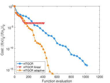
(a) Number of function evaluations vs. relative residual norm.

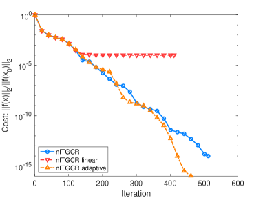
(b) Number of iterations vs. relative residual norm.

Figure 1: Comparison between the standard, linearized update, and adaptive update versions of nlTGCR(m) with $m=1$ on the Bratu problem. Each marker represents 20 iterations.

The Bratu problem has the property of being almost linear despite the presence of an exponential term. This property also appears in many applications when nearing convergence. Therefore, it is worth considering the linearized residual version of nlTGCR(m) ($\>8a$ in Section 4.1) as it can substantially reduce the number of required function evaluations. However, the linear update version is generally less robust than the nonlinear one. To address this issue and still benefit from the reduced number of function evaluations, we introduce an adaptive update version that balances the robustness and efficiency of nlTGCR(m).

Adaptive update

We introduce a residual check mechanism that determines when to switch from the nonlinear update to the linear update, as well as when to switch back. Let $r^{nl}_{j}$ and $r^{lin}_{j}$ denote the nonlinear and linear residuals at iteration $j$, respectively:

(69) $$r^{nl}_{j+1}=-f(x_{j+1}),\ \ r^{lin}_{j+1}=r^{nl}_{j}-V_{j}y_{j}.$$

We define an ‘angular distance’ between the nonlinear and linear residuals:

(70) $$\theta_{j}:=1-\frac{(r^{nl}_{j})^{T}r^{lin}_{j}}{\|r^{nl}_{j}\|_{2}\cdot\|r^{lin}_{j}\|_{2}}.$$

We choose a threshold $\theta$ which is set to $\theta=0.01$ in this paper. Then the linear update version will be switched on when $\theta_{j}<\theta$. We also check if $\theta_{j}\geq\theta$ on a regular basis, for example, every 10 iterations, to determine if we should switch back to the nonlinear version. Note that when switching back from the linear version to the nonlinear version, the previous vectors $P_{j}$ and $V_{j}$ are cleared, and nlTGCR(m) starts anew with a starting point $x_{j}$. This mechanism can significantly reduce the total number of function evaluations without sacrificing convergence and accuracy.

For the experiment in Figure 1, the window size is $m=1$, and the starting point is a vector of all-ones $x_{0}=\textbf{1}$. The cost/objective is the relative residual norm $\|f(x)\|_{2}/\|f(x_{0})\|_{2}$. We compare all three types of residual update schemes in terms of the number of function evaluations and present results in Figure 1(a). It can be observed that the convergence rate of the adaptive update version is close to that of the linearized updated version in the first few iterations. This is because the adaptive update version switches to linear updates at the second iteration and switches back to the nonlinear form at the 110th iteration where the linear update version stalls. As for the cost (Y-axis) of each iteration, Figure 1(b) indicates that all three versions decrease almost in the same way per iteration before the onset of stagnation. The adaptive update version performs as well as the nonlinear update version afterward. Sections 5.1.2 and 5.2 report on more experiments with the adaptive version of nlTGCR(m). In Sections 5.3 to 5.5 we utilize the standard (nonlinear) update version of nlTGCR(m) for deep learning tasks, as the proposed residual check is not applicable in a stochastic context.

5.1.2 Exploiting symmetry

We now investigate whether nlTGCR(m) takes advantage of short-term recurrences when the Jacobian is symmetric. Recall that in the linear case, GCR is mathematically equivalent to the Conjugate Residual (CR) algorithm when the matrix is symmetric. In this situation a window size $m=1$ is optimal [63]. We tested nlTGCR(m) along with baselines including Nesterov’s Accelerated Gradient [55], L-BFGS [48], AA, Nonlinear Conjugate Gradient (NCG) of Fletcher–Reeves’ type [29], and Newton-CG [22]. Results are presented in Figures 2(a) and 2(b). We analyzed the convergence in terms of the number of function evaluations rather than the number of iterations because the backtracking line search is implemented for all methods considered except AA by default. We present the results of the first 300 function evaluations for all methods. The window size for nlTGCR(m) is $m=1$, while for L-BFGS and AA, it is $m=10$. The mixing parameter for AA is set to $\beta=0.1$ as suggested in [10]. For Newton-CG method, the maximum number of steps in the inner CG solve is 50. This inner loop can be terminated early if

(71) $$\|r_{k}\|\leq\eta\|f(x_{0})\|.$$

We choose the forcing term $\eta=0.9$ and adjust it via the Eisenstat-Walker method [25].

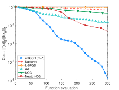
(a) Starting point $x_{0}=\textbf{0}$.

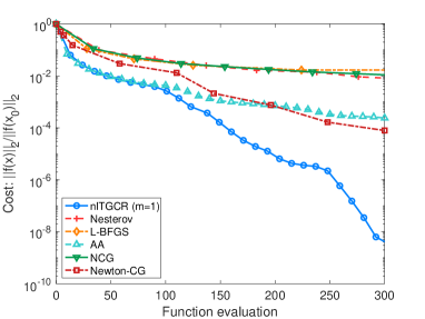
(b) Starting point $x_{0}=\textbf{1}$.

Figure 2: Number of function evaluations vs. relative residual norm on the Bratu problem with different starting points. Each marker represents 10 iterations except Newton-CG where each marker represents 1 outer loop step.

The Jacobian for the Bratu problem $\nabla f(s)$ is symmetric positive definite (SPD), making nlTGCR(m) with $m=1$ a highly efficient method. Other methods that do not take advantage of this symmetry require a larger number of vectors to achieve comparable performance. We tested the methods with two different initial guesses. The first, used in the experiments in Figure 2(a), is $x_{0}=\textbf{0}$ which is somewhat close to the global optimum. The second initial guess, used in the experiments in Figure 2(b), is the vector of all ones $x_{0}=\textbf{1}$. In both cases, we set the window size of L-BFGS and AA to 10, which means that 20 vectors in addition to $x_{j}$ and $r_{j}$ need to be stored. In contrast, nlTGCR(m=1) only requires 2 extra vectors. In this problem, nlTGCR(m=1), Nesterov, NCG, and Newton-CG are memory-efficient in terms of the number of vectors required to store information from previous steps. Among these competitive methods, nlTGCR($m=1$) performs best – suggesting that nlTGCR(m) benefits from symmetry.

5.2 Molecular optimization with Lennard-Jones potential

The second experiment focuses on the molecular optimization with the Lennard-Jones (LJ) potential which is a geometry optimization problem. The goal is to find atom positions that minimize total potential energy as described by the LJ potential:

(72) $$E=\sum_{i=1}^{N}\sum_{j=1}^{i-1}4\times\left[\frac{1}{\|y_{i}-y_{j}\|^{12}}-\frac{1}{\|y_{i}-y_{j}\|^{6}}\right].$$

In the above expression each $y_{i}$ is a 3-dimensional vector whose components are the coordinates of the location of atom $i$. We start with a certain configuration and then optimize the geometry by minimizing the potential starting from that position. Note that the resulting position is not a global optimum - it is just a local minimum around the initial configuration (see, e.g., Figure 3(a)). In this particular example, we simulate an Argon cluster by taking the initial position of the atoms to consist of a perturbed initial Face-Centered-Cubic (FCC) structure [54]. We took 3 cells per direction - resulting in 27 unit cells. FCC cells include 4 atoms each and so we end up with a total of 108 atoms. The problem is rather hard due to the high powers in the potential. In this situation backtracking or some form of line search is essential.

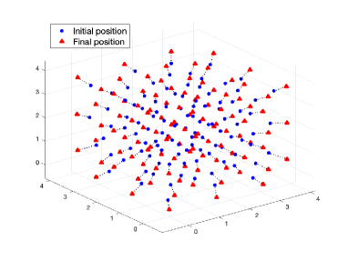
(a) Geometrical configurations.

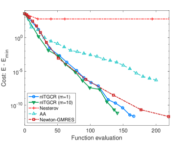
(b) Convergence of various methods.

Figure 3: (a) Initial and final configurations of 108 atoms with the Argon cluster experiment. (b) Number of function evaluations vs. shifted potential norm on the Lennard-Jones problem. Each marker represents 10 iterations for all methods except Newton-GMRES where each marker represents 1 outer loop step.

In this experiment, we set $f=\nabla E$. Each iterate in nlTGCR(m) is a vectorized array of coordinates of all atoms put together. So, it is a flat vector of length $3\times 108=324$. We present the results of the first 220 function evaluations for nlTGCR(m), AA, Nesterov, and Newton-GMRES in Figure 3(b). The reason for excluding L-BFGS, NCG, and Newton-CG is that the Jacobian/Hessian of the LJ problem is indefinite at some $x_{j}$ which can lead to a non-descending update direction. The window sizes for nlTGCR(m) are $m=1$ and $m=10$, while for AA it is $m=10$ and for Newton-GMRES it is $m=20$. This is because nlTGCR(m) and AA require storing twice as many additional vectors as the window size to generate the searching subspace, while Newton-GMRES does not. For each inner GMRES solve, GMRES is allowed to run up to 40 steps and utilizes a forcing term $\eta=0.9$ to terminate the inner loop. Moreover, AA does not converge unless the underlying fixed-point iteration $s_{j+1}=s_{j}+\beta f(s_{j})$ is carefully chosen. In this experiment, we select $\beta=10^{-3}$. The cost (Y-axis) represents the shifted potential $E-E_{min}$, where $E_{min}$ is the minimal potential achieved by all methods, approximately equal to $-579.4638$.

In Figure 3(b), we observe that nlTGCR($m=10$) converges the fastest. The convergence of nlTGCR($m=1$) and Newton-GMRES with a subspace dimension of 20 is close and slightly slower than nlTGCR($m=10$). One observed phenomenon worth mentioning is the quick termination of the inner loop of Newton-GMRES during the first few iterations. Newton-GMRES moves quickly to the next Jacobian at the beginning and focuses on a single Jacobian when nearing convergence. This behavior is made possible by the use of the Eisenstat-Walker technique, which accounts for the fast convergence of Newton-GMRES. However, without this early stopping mechanism, Newton-GMRES will fail to converge. In contrast, nlTGCR(m) and AA do not exclusively rely on one Jacobian at each iteration.

5.3 Image classification using ResNet

We now test the usefulness of nlTGCR(m) for deep learning applications by first comparing it with two commonly used optimization algorithms, Adam [44] and momentum. We report the training loss (MSE) and test accuracy on the CIFAR10 dataset [46] using ResNet [38]. We employed a ResNet 18 architecture from Pytorch . The window size $m$ is 1 for nlTGCR(m) because we found a large window size did not help improve the convergence too much in our preliminary experiments. The hyperparameters of the baseline methods are set to be the same as suggested in [38], i.e., the learning rate is 0.001 and 0.1 for Adam and momentum, respectively. Figure 4(a) depicts the training loss over time for each optimization algorithm, and Figure 4(b) shows the corresponding test accuracy. As can be seen nlTGCR($m=1$) achieved the best performance in terms of both convergence speed and accuracy. The experimental results revealed that nlTGCR outperformed the baseline methods by a significant margin. It is worth noting that nlTGCR converges to a loss of 0 for this problem, which empirically verifies the theoretically established global convergence properties of the method. This suggests that nlTGCR($m=1$) may lead to an interesting alternative to the state-of-the-art optimization methods in deep learning.

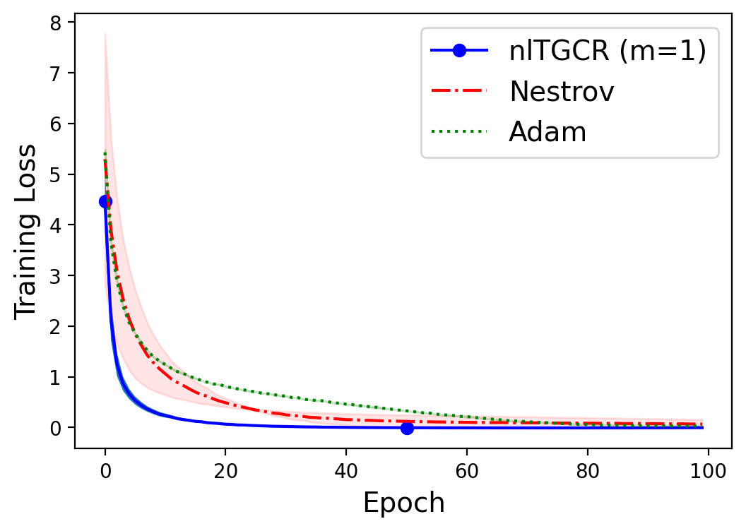
(a) Training Loss

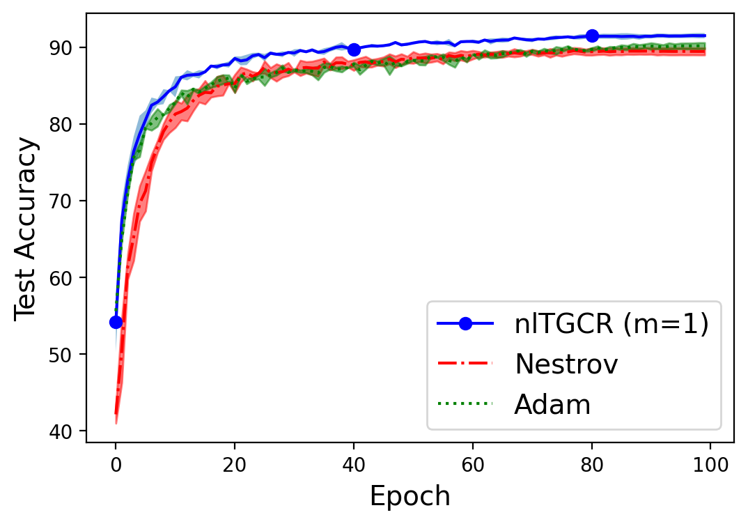
(b) Test Accuracy

Figure 4: Image Classification on CIFAR10 using ResNet (Averaged over 5 independent runs). nlTGCR(m=1), Adam, and momentum achieved a test accuracy of $91.56\%,90.13\%,89.53\%$ respectively.

5.4 Learning dynamic using Neural-ODE solver

We conducted experiments using a Neural-ODE solver [18] to learn underlying dynamic ODEs from sampled data. In our work, we focused on studying the spiral function

$$\frac{dz}{dt}=[-0.1,-1.0;1.0,-0.1]z,$$

which is a challenging dynamic to fit and is often used as a benchmark for testing the effectiveness of machine learning algorithms. We generated the training data by randomly sampling points from the spiral and adding small amounts of Gaussian noise. The goal was to train the model to generate data-like trajectories.

However, training such a model is computationally expensive. Therefore, we introduced nlTGCR(m) to recover the spiral function quickly and accurately, with the potential for better generalization to other functions. Our experiments involved training and evaluating a neural-ODE model on the sampled dataset for the spiral function compared with Adam and momentum. After a grid-search, we set the learning rate as 0.01 for Adam and window size $m=1$ for nlTGCR(m). We reported the mean squared error (MSE) training loss and visualized the model’s ability to recover the dynamic in Figure 5. We did not visualize the momentum as it took over 100 epochs to converge.

Figure 5(a) shows that nlTGCR(m=1) converges faster and more stably than Adam. Additionally, Figures 5(b) and 5(c) demonstrate that nlTGCR(m=1) is capable of generating data-like trajectories in just 15 epochs, whereas Adam struggles to converge even after 50 epochs. This experiment demonstrates the superiority of nlTGCR($m=1$) for this interesting application, relative to commonly used optimizers such as Adam and momentum.

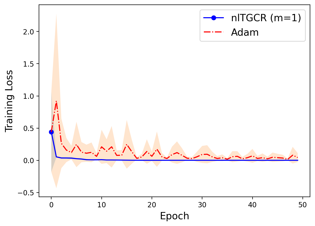
(a) Training Loss

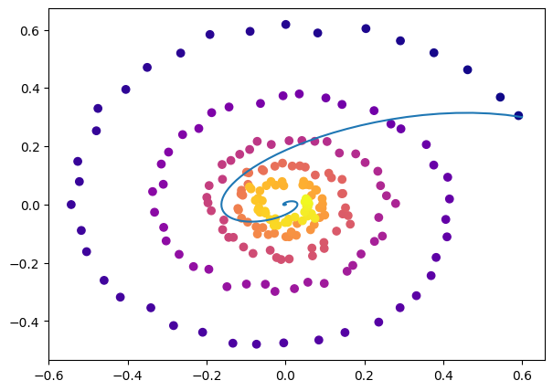
(b) Adam after 50 epochs

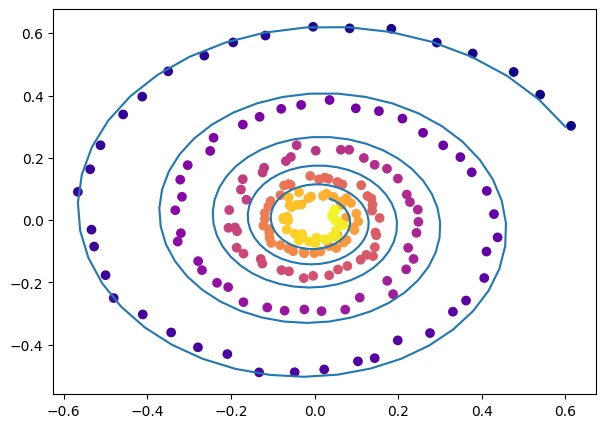
(c) nlTGCR(m=1) after 15 epochs

Figure 5: Learning true dynamic using Neural ODE. It can be observed that nlTGCR(m=1) converges much faster and can recover the true dynamic up to 5$\times$ faster than Adam.

5.5 Node classification using Graph Convolutional Networks

Finally, we explore the effectiveness of nlTGCR(m) in deep learning applications by implementing graph convolutional networks (GCNs) [45]. We use the commonly used Cora dataset [52] which contains 2708 scientific publications on one of 7 topics. Each publication is described by a binary vector of 1433 unique words indicating the absence or presence in the dictionary. This network consists of 5429 links representing the citation. The objective is a node classification via words and links. The neural network has one GCN layer and one dropout layer of rate 0.5. We adopted the GCN implementation directly from PyTorch-Geometric [3].

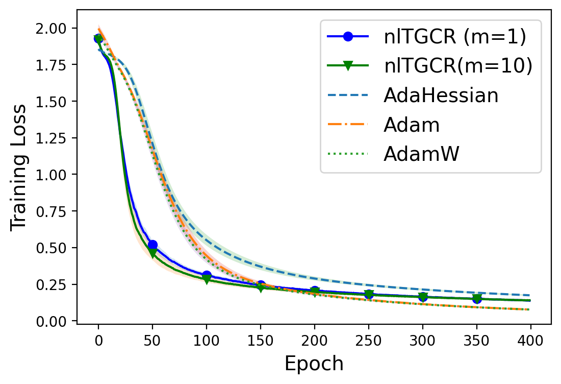
(a) Training Loss

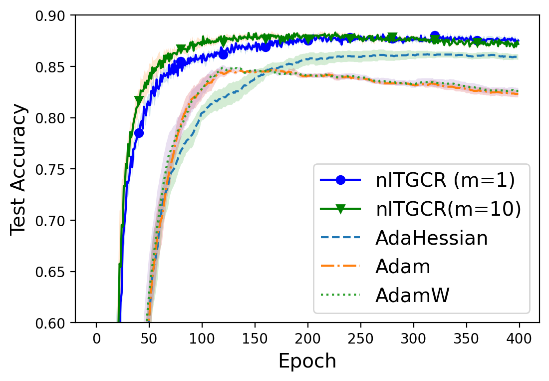
(b) Test Accuracy

Figure 6: GCN on Cora. nlTGCR(m=1) achieved a test accuracy of $88.13\%$, which is $4.02\%$ higher than the second best baseline AdamW.

We set $m=1$ in nlTGCR(m) and compare it with Adam [43], AdamW [49], and AdaHessian [79] with learning rates $lr=0.01,0.01,0.003$ respectively after a grid search. We present results of the training loss (Cross Entropy) and test accuracy in Figure 6(a) and 6(b). Note that a lower loss function does not necessarily means a better solution or convergence because of the bias and variance trade-off. Although Adam achieved a lower training loss, it is not considered as a better solution because its poor generalization capability on unseen datasets. We can observe that nlTGCR($m=1$) shows the best performance in this task. Specifically, it is not necessary to use a large window size since there is no significant difference between $m=1$ and $m=10$. This experiment shows again that nlTGCR($m=1$) can be adapted to the solution of DL problems.

6 Concluding remarks

The initial goal of this study was primarily to seek to develop Anderson-like methods that can take advantage of the symmetry of the Hessian in optimization problems. What we hope to have conveyed to the reader is that, by a careful extension of linear iterative schemes, one can develop a whole class of methods, of which nlTGCR(m) is but one member, that can be quite effective, possibly more so than many of the existing techniques in some situations. We are cautiously encouraged by the results obtained for Deep Learning problems although much work remains to be done to adapt and further test nlTGCR(m) for the stochastic context. In fact, our immediate research plan is precisely to perform such an in-depth study that focuses on Deep Learning applications.

7 Appendix A: More on GCR for solving linear systems

A number of results on the GCR algorithm for linear systems are known but their statements or proofs are not readily available from a single source. For example, it is intuitive, and well-known, that when $A$ is Hermitian then GCR will simplify to its CG-like algorithm known as the Conjugate Residual algorihm, but a proof cannot be easily found. This section summarizes the most important ones of these results with an emphasis on a unified presentation that exploits a matrix formalism.

7.1 Conjugacy and orthogonality relations

We start with Algorithm 1 where we assume no truncation ($m=\infty$). It is convenient to use a matrix formalism for the purpose of unraveling some relations and so we start by defining:

(73) $$R_{k}=[r_{0},r_{1},\cdots,r_{k}].$$

The relation in Line 7 of the algorithm can be rewritten in matrix form as follows:

(74) $$R_{k}=P_{k}B^{({k})},$$

where $B^{({k})}$ is an upper triangular matrix of size $(k+1)\times(k+1)$ defined as follows

(75) $$B^{({k})}\in\mathbb{R}^{(k+1)\times(k+1)},\qquad B^{({k})}_{ij}=\left\{\begin{array}[]{lcl}0&\text{if}&i>j\\ 1&\text{if}&i=j\\ \beta_{(i-1),(j-1)}&\text{if}&i<j\end{array}\right.$$

Similarly, note that the relation from Line 6 of the algorithm can be recast as:

(76) $$AP_{k}=R_{k+1}\underline{H}^{({k})},$$

where $\underline{H}^{({k})}$ is a $(k+2)\times(k+1)$ lower bidiagonal matrix with

(77) $$\underline{H}^{({k})}_{ij}=\left\{\begin{array}[]{lcl}\frac{1}{\alpha_{j-1}}&\text{if}&i=j\\ \frac{-1}{\alpha_{j-1}}&\text{if}&i=j+1\\ 0&\text{if}&i<j\ \text{or}\ i>j+1\end{array}\right.$$

Proposition 7.1.

(Eisenstat-Elman-Schultz [23]) The residual vectors produced by (full) GCR are semi-conjugate.

Proof 7.2.

Semi-conjugacy means that each $r_{j}$ is orthogonal to $Ar_{0},Ar_{1},\cdots Ar_{j-1}$, so we need to show that $R_{k}^{T}AR_{k}$ is upper triangular. We know that each $r_{j+1}$ is orthogonal to $Ap_{i}$ for $i=1,\cdots,j$ a relation we write as

(78) $$R_{k}^{T}AP_{k}=U_{k}$$

where $U_{k}$ is some upper triangular matrix. Then, from (74) we have $AR_{k}=AP_{k}B^{({k})}$ and therefore:

(79) $$R_{k}^{T}AR_{k}=R_{k}^{T}AP_{k}B^{({k})}=U_{k}B^{({k})}$$

which is upper triangular as desired.

We get an immediate consequence of this result for the case when $A$ is Hermitian.

Corollary 7.3.

When $A$ is symmetric real (Hermitian complex) then the directions $\{r_{j}\}$, are $A$-conjugate.

Proof 7.4.

Indeed, when $A$ is symmetric real the matrix $R_{k}^{T}AR_{k}=U_{k}B^{({k})}$ is also symmetric and since it is upper triangular it must be diagonal which shows that the $r_{j}$’s are $A$-conjugate.

In this situation, we can write

(80) $$R_{k}^{T}AR_{k}=D_{k},$$

where $D_{k}$ is a $(k+1)\times(k+1)$ diagonal matrix. The next result shows that the algorithm simplifies when $A$ is symmetric. Specifically, the scalars $\beta_{ij}$ needed in the orthgonalization in Line 7 are all zero except $\beta_{jj}$.

Proposition 7.5.

When $A$ is symmetric real, then the matrix $(AR_{k})^{T}(AP_{k})$ is lower bidiagonal.

Proof 7.6.

As a result of (76) the matrix $(AR_{k})^{T}(AP_{k})$ is:

$$(AR_{k})^{T}(AP_{k})=(AR_{k})^{T}R_{k+1}\underline{H}^{({k})}.$$

Observe that $(AR_{k})^{T}R_{k+1}=[D_{k},0_{(k+1)\times 1}]$ and the product $[D_{k},0_{(k+1)\times 1}]\underline{H}^{({k})}$ yields the $(k+1)\times(k+1)$ matrix obtained from $\underline{H}^{({k})}$ but deleting its last row which we denote by $H^{({k})}$. Therefore,

$$(AR_{k})^{T}(AP_{k})=D_{k}H^{({k})}$$

is a $(k+1)\times(k+1)$ bidiagonal matrix.

7.2 Break-down of GCR

Next we examine the conditions under which the full GCR breaks down.

Proposition 7.7.

When $A$ is nonsingular, the only way in which (full) GCR breaks down is when it produces an exact solution. In other words its only possible breakdown is the so-called ‘lucky breakdown’.

Proof 7.8.

The algorithm breaks down only if $Ap_{j+1}$ produced in Line 7 is zero, i.e., when $p_{j+1}==0$ since $A$ is nonsingular. In this situation $r_{j+1}=\sum_{i=0}^{j}\beta_{ij}p_{i}$. It can be easily seen that each $p_{i}$ is of the form $p_{i}=\mu_{i}(A)r_{0}$ where $\mu_{i}$ is a polynomial of degree $i$. Similarly $r_{j+1}=\rho_{j+1}(A)r_{0}$ in which $\rho_{j+1}$ is a polynomial of degree (exactly) $j+1$. Therefore, the polynomial $\pi_{j+1}(t)\equiv\rho_{j+1}(t)-\sum_{i=0}^{j}\beta_{ij}\mu_{i}(t)$ is a polynomial of degree exactly $j+1$ such that $\pi_{j+1}(A)r_{0}=0$. Thus, the degree of the minimal polynomial for $r_{0}$ is $j+1$ and we are in the standard situation of a lucky breakdown. Indeed, since the algorithm produces a solution $x_{j+1}$ that minimizes the residual norm, and because the degree of the minimal polynomial for $r_{0}$ is equal to $j+1$ we must have $r_{j+1}=0$.

Note that the proposition does not state anything about convergence. The iterates that are computed will have a residual norm that is non-increasing but the iterates may stagnate. Convergence can be shown in the case when $A$ is positive definite, i.e., when its symmetric part is SPD.

In addition, the proof of this result requires that the solution that is produced has a minimal residual which is not the case for the truncated version. Thus, in the truncated version, we may well have a situation where $p_{j+1}=0$ but the solution $x_{j+1}$ is not exact. If we had $p_{j+1}=0$ it would mean that $\eta_{j+1}(A)r_{0}=0$, i.e., the minimal polynomial for $r_{0}$ is again of degree exactly $j+1$. This is an unlikely event which we may term ‘unlucky breakdown’. However, in practice the more common situation that can take place is to get a vector $p_{j+1}$ with small norm.

Suppose now that $A$ is positive definite, i.e. that its symmetric part is SPD. Let us assume that $p_{k}=0$ but $r_{k}\neq 0$ – which represents the scenario of an ‘unlucky breakdown’ at step $k$. Then since the last column of $P_{k}$ is a zero vector the last column of the matrix $U_{k}$ in (78) is also zero. This in turn would imply that the last row of the product $U_{k}B^{({k})}$ in (79) is zero. However, this can’t happen because according to (79) it is equal to the last row of the matrix $R_{k}^{T}AR_{k}$ where $A$ is positive definite. Thus, the ‘unlucky breakdown’ scenario invoked above is only possible when $A$ is indefinite.

7.3 Properties of the induced approximate inverse

When $x_{0}=0$ the approximate solution obtained at the end of the algorithm is of the form $x_{k+1}=P_{k}V_{k}^{T}b$. We say that the algorithm induces the approximation $B_{k}=P_{k}V_{k}^{T}$ to the inverse of $A$. Note that even in the case when $A$ is symmetric, $B_{k}$ is not symmetric in general. However, $B_{k}$ obeys a few easy to prove properties stated next.

Proposition 7.9.

Let $\mathcal{L}_{k}=\mbox{Span}(V_{k})$ and let $\pi=V_{k}V_{k}^{T}$ be the orthogonal projector onto $\mathcal{L}_{k}$. The (full) GCR algorithm induces the approximate inverse $B_{k}=P_{k}V_{k}^{T}$ which satisfies the following properties:

1. $B_{k}=A^{-1}\pi$

2. $B_{k}$ inverts $A$ exactly in $\mathcal{L}_{k}$, i.e., $B_{k}x=A^{-1}x$ for $x\in\mathcal{L}_{k}$. Equivalently, $B_{k}\pi=A^{-1}\pi$.

3. $AB_{k}$ equals the orthogonal projector $\pi$.

4. When $A$ is symmetric then $B_{k}$ is self-adjoint when restricted to $\mathcal{L}_{k}$.

5. $B_{k}Ax=x$ for any $x\in\mbox{Span}\{P_{k}\}$, i.e., $B_{k}$ inverts $A$ exactly from the left when $A$ is restricted to the range of $P_{k}$.

6. $B_{k}A$ is the projector onto $\mbox{Span}\{P_{k}\}$ and orthogonally to $A^{T}\mathcal{L}_{k}$.

Proof 7.10.

(1) The first property follows from the relation $AP_{k}=V_{k}$ and the definition of $B_{k}$.

(2) To prove the second property we write a member of $\mbox{Span}(V_{k})$ as $x=V_{k}y$. Then from the previous property we have

$$B_{k}x=A^{-1}V_{k}V_{k}^{T}V_{k}y=A^{-1}V_{k}y=A^{-1}x.$$

(3) $AB_{k}=AP_{k}V_{k}^{T}=V_{k}V_{k}^{T}=\pi$.

(4) The self-adjointness of $B_{k}$ in $\mathcal{L}_{k}$ is a consequence of (2). It can also be readily verified as follows. For any vectors $x,y\ \in\ \mathcal{L}_{k}$ write:

$$(B_{k}x,y)=(A^{-1}\pi x,y)=(A^{-1}x,y)=(x,A^{-1}y)=(x,A^{-1}\pi y)=(x,B_{k}y).$$

(5) Let a member of $\mbox{Span}(P_{k})$ be written as $x=P_{k}y$ and apply $B_{k}A$ to $x$:

$$B_{k}Ax=B_{k}AP_{k}y=B_{k}V_{k}y=A^{-1}V_{k}V_{k}^{T}V_{k}y=A^{-1}V_{k}y=P_{k}y=x.$$

Therefore, $B_{k}A$ leaves vectors of $\mbox{Span}(P_{k})$ unchanged.

(6) Because $B_{k}A$ leaves vectors of $\mbox{Span}(P_{k})$ unchanged it is a projector, call it $\pi_{O}$ (for oblique), with $\text{Ran}(\pi_{O})=\mbox{Span}\{P_{k}\}$. We now need to show that $(u-\pi_{O}u)\perp A^{T}\mathcal{L}_{k}$ for any $u$. Since $A^{T}V_{k}$ is a basis for $A^{T}\mathcal{L}_{k}$, this is equivalent to showing that $(A^{T}V_{k})^{T}(u-\pi_{O}u))=0$ for any $u$. We have for any given vector $u\in\mathbb{R}^{n}$

$$(A^{T}V_{k})^{T}(u-\pi_{O}u) =V_{k}^{T}(Au-AP_{k}V_{k}^{T}Au)=V_{k}^{T}(Au-V_{k}V_{k}^{T}Au)$$

$$=V_{k}^{T}(I-V_{k}V_{k}^{T})Au=0.$$

Thus (4) and (6) indicate that while $AB_{k}$ is an orthogonal projector, $B_{k}A$ is an oblique projector. Although (4) is an obvious consequence of (3), it is interesting to note that it is rather similar to relations obtained in the context of Moore-Penrose pseudo-inverses.

8 Appendix B: Convergence analysis

We provide an alternative analysis of the global convergence of nlTGCR based on the backtracking line search strategy. We will make the following assumptions:

Assumption A:

(81) $$\text{ The set}~{}S=\{x:\phi(x)\leq\phi(x_{0})\}~{}\text{is bounded};$$

Assumption B:

(82) $$\nabla\phi~{}\text{is L-Lipschitz},\|\nabla\phi(x)-\nabla\phi(y)\|\leq L\|x-y\|,~{}0<L<\infty.$$

Assumption C: There exists a $\gamma>0$ such that $d_{j}$ produced by Algorithm 2 satisfies

(83) $$-\frac{d_{j}^{\top}\nabla\phi(x_{j})}{\|d_{j}\|\|\nabla\phi(x_{j})\|}\geq\gamma>0,\forall j$$

Assumption D: There exist two positive constants $\mu$ and $\Theta$ such that,

(84) $$\|d_{j}\|\geq\mu\|\nabla\phi(x_{j})\|,\quad\|d_{j}\|\leq\Theta,\forall j.$$

Theorem 8.1.

For any scalar function $\phi(x)$, consider the iterates $x_{j+1}=x_{j}+\alpha_{j}d_{j}$ with descent directions $d_{j}$ produced by Algorithm 2 and stepsizes $\alpha_{j}$ produced by backtracking line search (49). Suppose assumptions (A-D) also hold, then

(85) $$\lim_{j\rightarrow\infty}\|\nabla\phi(x_{j})\|=0.$$

This theorem is a well-known result in optimization and it can be found in various sources, including [32]. We omit its proof.

References

- [1] hiroyuki-kasai/GDLibrary. https://github.com/hiroyuki-kasai/GDLibrary.
- [2] PyTorch. https://www.pytorch.org.
- [3] PyTorch-Geometric. https://www.pyg.org/.
- [4] D. G. Anderson, Iterative procedures for non-linear integral equations, Assoc. Comput. Mach., 12 (1965), pp. 547–560.
- [5] L. Armijo, Minimization of functions having Lipschitz continuous first partial derivatives, Pacific Journal of Mathematics, 16 (1966), pp. 1–3.
- [6] O. Axelsson, Conjugate gradient type-methods for unsymmetric and inconsistent systems of linear equations, Linear Algebra and its Applications, 29 (1980), pp. 1–16.
- [7] W. Bian, X. Chen, and C. T. Kelley, Anderson acceleration for a class of nonsmooth fixed-point problems, SIAM Journal on Scientific Computing, 43 (2021), pp. S1–S20.
- [8] N. Boutet, R. Haelterman, and J. Degroote, Secant update version of quasi-Newton PSB with weighted multisecant equations, Computational Optimization and Applications, 75 (2020), pp. 441–466.
- [9] , Secant update generalized version of PSB: a new approach, Computational Optimization and Applications, 78 (2021), pp. 953–982.
- [10] C. Brezinski, S. Cipolla, M. Redivo-Zaglia, and Y. Saad, Shanks and Anderson-type acceleration techniques for systems of nonlinear equations, IMA Journal of Numerical Analysis, 42 (2022), pp. 3058–3093.
- [11] C. Brezinski and M. Redivo-Zaglia, The simplified topological -algorithms for accelerating sequences in a vector space, SIAM Journal on Scientific Computing, 36 (2014), pp. A2227–A2247.
- [12] C. Brezinski, M. Redivo-Zaglia, and Y. Saad, Shanks sequence transformations and Anderson acceleration, SIAM Review, 60 (2018), pp. 646–669.
- [13] P. N. Brown and Y. Saad, Hybrid Krylov methods for nonlinear systems of equations, SIAM J. Sci. Stat. Comp., 11 (1990), pp. 450–481.
- [14] , Convergence theory of nonlinear Newton-Krylov algorithms, SIAM Journal on Optimization, 4 (1994), pp. 297–330.
- [15] A. Cabana and L. F. Lago-Fernández, Backward gradient normalization in deep neural networks, 2021.
- [16] S. Cabay and L. W. Jackson, A polynomial extrapolation method for finding limits and antilimits of vector sequences, SIAM Journal on Numerical Analysis, 13 (1976), pp. 734–752.
- [17] M. H. Chaudhry et al., Open-channel flow, vol. 523, Springer, 2008.
- [18] R. T. Q. Chen, Y. Rubanova, J. Bettencourt, and D. Duvenaud, Neural ordinary differential equations, 2019.
- [19] M. Chupin, M.-S. Dupuy, G. Legendre, and E. Séré, Convergence analysis of adaptive DIIS algorithms with application to electronic ground state calculations, ESAIM: Mathematical Modelling and Numerical Analysis, 55 (2021), pp. 2785–2825.
- [20] A. d’Aspremont, D. Scieur, and A. Taylor, Acceleration methods, Foundations and Trends® in Optimization, 5 (2021), pp. 1–245.
- [21] J. Degroote, K.-J. Bathe, and J. Vierendeels, Performance of a new partitioned procedure versus a monolithic procedure in fluid-structure interaction, Comput. & Structures, 87 (2009), pp. 798–801.
- [22] R. S. Dembo, S. C. Eisenstat, and T. Steihaug, Inexact Newton methods, SIAM J. Numer. Anal., 18 (1982), pp. 400–408.
- [23] S. C. Eisenstat, H. C. Elman, and M. H. Schultz, Variational iterative methods for nonsymmetric systems of linear equations, SIAM Journal on Numerical Analysis, 20 (1983), pp. 345–357.
- [24] S. C. Eisenstat and H. F. Walker, Globally convergent inexact Newton methods, SIAM Journal on Optimization, 4 (1994), pp. 393–422.
- [25] S. C. Eisenstat and H. F. Walker, Choosing the forcing terms in an inexact Newton method, SIAM Journal on Scientific Computing, 17 (1996), pp. 16–32.
- [26] C. Evans, S. Pollock, L. G. Rebholz, and M. Xiao, A proof that Anderson acceleration improves the convergence rate in linearly converging fixed-point methods (but not in those converging quadratically), SIAM Journal on Numerical Analysis, 58 (2020), pp. 788–810.
- [27] V. Eyert, A comparative study on methods for convergence acceleration of iterative vector sequences, J. Computational Phys., 124 (1996), pp. 271–285.
- [28] J.-L. Fattebert, Accelerated block preconditioned gradient method for large scale wave functions calculations in density functional theory, Journal of Computational Physics, 229 (2010), pp. 441–452.
- [29] R. Fletcher and C. M. Reeves, Function minimization by conjugate gradients, The computer journal, 7 (1964), pp. 149–154.
- [30] G. B. Folland, Introduction to partial differential equations, vol. 102, Princeton university press, 1995.
- [31] M. Geist and B. Scherrer, Anderson acceleration for reinforcement learning, 2018.
- [32] I. Griva, S. G. Nash, and A. Sofer, Linear and nonlinear optimization, vol. 108, Siam, 2009.
- [33] M. Hajipour, A. Jajarmi, and D. Baleanu, On the accurate discretization of a highly nonlinear boundary value problem, Numerical Algorithms, 79 (2018), pp. 679–695.
- [34] H. He, Y. Xi, and J. C. Ho, Fast and accurate tensor decomposition without a high performance computing machine, in 2020 IEEE International Conference on Big Data (Big Data), IEEE, 2020, pp. 163–170.
- [35] H. He, S. Zhao, Z. Tang, J. C. Ho, Y. Saad, and Y. Xi, An efficient nonlinear acceleration method that exploits symmetry of the Hessian, 2022.
- [36] H. He, S. Zhao, Y. Xi, and J. Ho, AGE: Enhancing the convergence on GANs using alternating extra-gradient with gradient extrapolation, in NeurIPS 2021 Workshop on Deep Generative Models and Downstream Applications.
- [37] H. He, S. Zhao, Y. Xi, J. Ho, and Y. Saad, GDA-AM: on the effectiveness of solving minimax optimization via Anderson mixing, in International Conference on Learning Representations, 2022.
- [38] K. He, X. Zhang, S. Ren, and J. Sun, Deep residual learning for image recognition, 2015.
- [39] K. Jbilou and H. Sadok, LU implementation of the modified minimal polynomial extrapolation method for solving linear and nonlinear systems, IMA Journal of Numerical Analysis, 19 (1999), pp. 549–561.
- [40] K. C. Jea and D. M. Young, Generalized conjugate gradient acceleration of nonsymmetrizable iterative methods, Linear Algebra and its Applications, 34 (1980), pp. 159–194.
- [41] C. T. Kelley, Iterative methods for linear and nonlinear equations, Volumne 16 of Frontiers and Applied Mathematics, SIAM, Philadelphia, PA, 1995.
- [42] C. T. Kelley, Solving nonlinear equations with Newton’s method, Society for Industrial and Applied Mathematics, Jan. 2003.
- [43] D. P. Kingma and J. Ba, Adam: a method for stochastic optimization, arXiv preprint arXiv:1412.6980, (2014).
- [44] D. P. Kingma and J. Ba, Adam: A method for stochastic optimization, 2017.
- [45] T. N. Kipf and M. Welling, Semi-supervised classification with graph convolutional networks, arXiv preprint arXiv:1609.02907, (2016).
- [46] A. Krizhevsky, Learning multiple layers of features from tiny images, 2009.
- [47] L. Lin and C. Yang, Elliptic preconditioner for accelerating the self-consistent field iteration in Kohn–Sham density functional theory, SIAM Journal on Scientific Computing, 35 (2013), pp. S277–S298.
- [48] D. C. Liu and J. Nocedal, On the limited memory BFGS method for large scale optimization, Mathematical programming, 45 (1989), pp. 503–528.
- [49] I. Loshchilov and F. Hutter, Decoupled weight decay regularization, 2019.
- [50] V. Mai and M. Johansson, Anderson acceleration of proximal gradient methods, in Proceedings of the 37th International Conference on Machine Learning, H. D. III and A. Singh, eds., vol. 119 of Proceedings of Machine Learning Research, PMLR, 13–18 Jul 2020, pp. 6620–6629.
- [51] V. V. Mai and M. Johansson, Nonlinear acceleration of constrained optimization algorithms, in ICASSP 2019 - 2019 IEEE International Conference on Acoustics, Speech and Signal Processing (ICASSP), 2019, pp. 4903–4907.
- [52] A. K. McCallum, K. Nigam, J. Rennie, and K. Seymore, Automating the construction of internet portals with machine learning, Information Retrieval, 3 (2000), pp. 127–163.
- [53] G. Meurant and J. D. Tebbens, Krylov methods for nonsymmetric linear systems - from theory to computations, Springer Series in Computational Mathematics, vol. 57, Springer, 2020.
- [54] L. Meyer, C. Barrett, and P. Haasen, New crystalline phase in solid argon and its solid solutions, The Journal of Chemical Physics, 40 (1964), pp. 2744–2745.
- [55] Y. Nesterov, Introductory lectures on convex optimization: a basic course, Springer Publishing Company, Incorporated, 1 ed., 2014.
- [56] C. W. Oosterlee and T. Washio, Krylov subspace acceleration of nonlinear multigrid with application to recirculating flows, SIAM Journal on Scientific Computing, 21 (2000), pp. 1670–1690.
- [57] M. L. Pasini, J. Yin, V. Reshniak, and M. K. Stoyanov, Anderson acceleration for distributed training of deep learning models, in SoutheastCon 2022, 2022, pp. 289–295.
- [58] S. Pollock, L. G. Rebholz, and M. Xiao, Anderson-accelerated convergence of Picard iterations for incompressible navier–stokes equations, SIAM Journal on Numerical Analysis, 57 (2019), pp. 615–637.
- [59] M. POWELL, A new algorithm for unconstrained optimization, in Nonlinear Programming, J. Rosen, O. Mangasarian, and K. Ritter, eds., Academic Press, 1970, pp. 31–65.
- [60] P. Pulay, Convergence acceleration of iterative sequences. the case of SCF iteration, Chem. Phys. Lett., 73 (1980), pp. 393–398.
- [61] , Improved SCF convergence acceleration, J. Comput. Chem., 3 (1982), pp. 556–560.
- [62] H. ren Fang and Y. Saad, Two classes of multisecant methods for nonlinear acceleration, Numerical Linear Algebra with Applications, 16 (2009), pp. 197–221.
- [63] Y. Saad, Iterative methods for sparse linear systems, 2nd edition, SIAM, Philadelpha, PA, 2003.
- [64] Y. Saad, Numerical methods for large eigenvalue problems-classics edition, SIAM, Philadelphia, 2011.
- [65] R. B. Schnabel, Quasi-Newton methods using multiple secant equations, Tech. Rep. CU-CS-247-83, Department of Computer Science, University of Colorado at Boulder, Boulder, CO, 1983.
- [66] D. Scieur, L. Liu, T. Pumir, and N. Boumal, Generalization of quasi-Newton methods: application to robust symmetric multisecant updates, in Proceedings of The 24th International Conference on Artificial Intelligence and Statistics, A. Banerjee and K. Fukumizu, eds., vol. 130 of Proceedings of Machine Learning Research, PMLR, 13–15 Apr 2021, pp. 550–558.
- [67] D. Scieur, E. Oyallon, A. d’Aspremont, and F. Bach, Online regularized nonlinear acceleration, 2018.
- [68] W. Shi, S. Song, H. Wu, Y. Hsu, C. Wu, and G. Huang, Regularized Anderson acceleration for off-policy deep reinforcement learning, in NeurIPS, 2019.
- [69] D. A. Smith, W. F. Ford, and A. Sidi, Extrapolation methods for vector sequences, SIAM Review, 29 (1987), pp. 199–233.
- [70] E. Stiefel, Relaxationsmethoden bester strategie zur lösung linearer gleichungssysteme, Commentarii Mathematici Helvetici, 29 (1955), pp. 157–179.
- [71] K. Sun, Y. Wang, Y. Liu, Y. Zhao, B. Pan, S. Jui, B. Jiang, and L. Kong, Damped Anderson mixing for deep reinforcement learning: acceleration, convergence, and stabilization, in NeurIPS, 2021.
- [72] A. Toth and C. T. Kelley, Convergence analysis for Anderson acceleration, SIAM Journal on Numerical Analysis, 53 (2015), p. 805–819.
- [73] D. Vanderbilt and S. G. Louie, Total energies of diamond (111) surface reconstructions by a linear combination of atomic orbitals method, Phys. Rev. B, 30 (1984), pp. 6118–6130.
- [74] P. K. W. Vinsome, ORTHOMIN: an iterative method for solving sparse sets of simultaneous linear equations, in Proceedings of the Fourth Symposium on Resevoir Simulation, Society of Petroleum Engineers of AIME, 1976, pp. 149–159.
- [75] H. F. Walker and P. Ni, Anderson acceleration for fixed-point iterations, SIAM J. Numer. Anal., 49 (2011), pp. 1715–1735.
- [76] F. Wei, C. Bao, and Y. Liu, Stochastic Anderson mixing for nonconvex stochastic optimization, 2021.
- [77] F. Wei, C. Bao, and Y. Liu, A class of short-term recurrence Anderson mixing methods and their applications, in International Conference on Learning Representations, 2022.
- [78] P. Wilmott, S. Howson, S. Howison, J. Dewynne, et al., The mathematics of financial derivatives: a student introduction, Cambridge university press, 1995.
- [79] Z. Yao, A. Gholami, S. Shen, K. Keutzer, and M. W. Mahoney, Adahessian: An adaptive second order optimizer for machine learning, AAAI (Accepted), (2021).
- [80] J. Zhang, B. O’Donoghue, and S. Boyd, Globally convergent type-I Anderson acceleration for non-smooth fixed-point iterations, 2018.