(Almost) Provable Error Bounds Under Distribution Shift via Disagreement Discrepancy

Abstract

We derive an (almost) guaranteed upper bound on the error of deep neural networks under distribution shift using unlabeled test data. Prior methods either give bounds that are vacuous in practice or give estimates that are accurate on average but heavily underestimate error for a sizeable fraction of shifts. In particular, the latter only give guarantees based on complex continuous measures such as test calibration—which cannot be identified without labels—and are therefore unreliable. Instead, our bound requires a simple, intuitive condition which is well justified by prior empirical works and holds in practice effectively 100% of the time. The bound is inspired by ${\mathcal{H}}\Delta{\mathcal{H}}$-divergence but is easier to evaluate and substantially tighter, consistently providing non-vacuous guarantees. Estimating the bound requires optimizing one multiclass classifier to disagree with another, for which some prior works have used sub-optimal proxy losses; we devise a “disagreement loss” which is theoretically justified and performs better in practice. We expect this loss can serve as a drop-in replacement for future methods which require maximizing multiclass disagreement. Across a wide range of benchmarks, our method gives valid error bounds while achieving average accuracy comparable to competitive estimation baselines.

1 Introduction

When deploying a model, it is important to be confident in how it will perform under inevitable distribution shift. Standard methods for achieving this include data dependent uniform convergence bounds (Mansour et al., 2009, Ben-David et al., 2006) (typically vacuous in practice) or assuming a precise model of how the distribution can shift (Rahimian and Mehrotra, 2019, Chen et al., 2022, Rosenfeld et al., 2021). Unfortunately, it is difficult or impossible to determine how severely these assumptions are violated by real data (“all models are wrong”), so practitioners usually cannot trust such bounds with confidence.

To better estimate test performance in the wild, some recent work instead tries to directly predict accuracy of neural networks using unlabeled data from the test distribution of interest, (Garg et al., 2022, Baek et al., 2022, Lu et al., 2023). While these methods predict the test performance surprisingly well, they lack pointwise trustworthiness and verifiability: their estimates are good on average over all distribution shifts, but they provide no guarantee or signal of the quality of any individual prediction (here, each point is a single test distribution, for which a method predicts a classifier’s average accuracy). Because of the opaque conditions under which these methods work, it is also difficult to anticipate their failure cases—indeed, it is reasonably common for them to substantially overestimate test accuracy for a particular shift, which is problematic when optimistic deployment can be costly or catastrophic. Worse yet, we find that this gap grows with test error (Figure 1), making these predictions least reliable under large distribution shift, which is precisely when their reliability is most important. Although it is clearly impossible to guarantee upper bounds on test error for all shifts, there is still potential for error bounds that are intuitive and reasonably trustworthy.

In this work, we develop a method for (almost) provably bounding test error of classifiers under distribution shift using unlabeled test points. Our bound’s only requirement is a simple, intuitive, condition which describes the ability of a hypothesis class to achieve small loss on a particular objective defined over the (unlabeled) train and test distributions. Inspired by ${\mathcal{H}}\Delta{\mathcal{H}}$-divergence (Ben-David et al., 2010), our method requires training a critic to maximize agreement with the classifier of interest on the source distribution while simultaneously maximizing disagreement on the target distribution; we refer to this joint objective as the disagreement discrepancy, and so we name the method Dis². We optimize this discrepancy over linear classifiers using deep features—or linear functions thereof—finetuned on only the training set. Recent evidence suggests that such representations are sufficient for highly expressive classifiers even under large distribution shift (Rosenfeld et al., 2022a). Experimentally, we find that our bound is valid effectively 100% of the time, consistently giving non-trivial lower bounds on test accuracy which are reasonably comparable to competitive baselines.

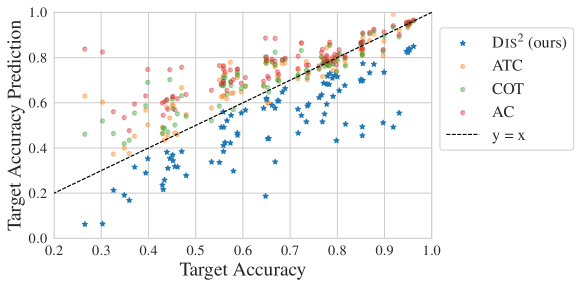
Figure 1: Our bound vs. three prior methods for estimation across a wide variety of distribution shift benchmarks (e.g., WILDs, BREEDs, DomainNet) and training methods (e.g., ERM, FixMatch, BN-adapt). Prior methods are accurate on average, but it is difficult or impossible to know when a given prediction is reliable and why. Worse yet, they usually overestimate accuracy, with the gap growing as test accuracy decreases—this is precisely when a reliable, conservative estimate is most desirable. Instead, Dis² maximizes the disagreement discrepancy to give a reliable error upper bound which holds effectively 100% of the time.

Additionally, we empirically show that it is even possible to approximately test this bound’s likelihood of being satisfied with only unlabeled data: the optimization process itself provides useful information about the bound’s validity, and we use this to construct a score which linearly correlates with the tightness of the bound. This score can then be used to relax the original bound into a sequence of successively tighter-yet-less-conservative estimates, interpolating between robustness and accuracy and allowing a user to make estimates according to their specific risk tolerance.

While maximizing agreement is statistically well understood, our method also calls for maximizing disagreement on the target distribution. This is not so straightforward in the multiclass setting, and we observe that prior works use unsuitable losses which do not correspond to minimizing the 0-1 loss of interest and are non-convex (or even concave) in the model logits (Chuang et al., 2020, Pagliardini et al., 2023). To rectify this, we derive a new “disagreement loss” which serves as an effective proxy loss for maximizing multiclass disagreement. Experimentally, we find that minimizing this loss results in lower risk (that is, higher disagreement) compared to prior methods, and we believe it can serve as a useful drop-in replacement for any future methods which require maximizing multiclass disagreement.

Experiments across numerous vision datasets (BREEDs (Santurkar et al., 2020), FMoW-WILDs (Koh et al., 2021), Visda (Peng et al., 2017), Domainnet (Peng et al., 2019), CIFAR10, CIFAR100 (Krizhevsky and Hinton, 2009) and OfficeHome (Venkateswara et al., 2017)) demonstrate the effectiveness of our bound. Though Dis² is competitive with prior methods for error estimation, we emphasize that our focus is not on improving raw predictive accuracy—rather, we hope to obtain reliable (i.e., conservative), reasonably tight bounds on the test error of a given classifier under distribution shift. In particular, while existing methods tend to severely overestimate accuracy as the true accuracy drops, our bound maintains its validity while remaining non-vacuous, even for drops in accuracy as large as 70%. In addition to source-only training, we experiment with unsupervised domain adaptation methods that use unlabeled target data and show that our observations continue to hold.

2 Related Work

Estimating test error with unlabeled data.

The generalization capabilities of overparameterized models on in-distribution data have been extensively studied using conventional machine learning tools (Neyshabur et al., 2015, 2017, Neyshabur, 2017, Neyshabur et al., 2018, Dziugaite and Roy, 2017, Bartlett et al., 2017, Zhou et al., 2018, Long and Sedghi, 2019, Nagarajan and Kolter, 2019a). This research aims to bound the generalization gap by evaluating complexity measures of the trained model. However, these bounds tend to be numerically loose compared to actual generalization error (Zhang et al., 2016, Nagarajan and Kolter, 2019b). Another line of work instead explores the use of unlabeled data for predicting in-distribution generalization (Platanios et al., 2016, 2017, Garg et al., 2021, Nakkiran and Bansal, 2019, Jiang et al., 2022b). More relevant to our work, there are several methods that predict the error of a classifier under distribution shift with unlabeled test data: (i) methods that explicitly predict the correctness of the model on individual unlabeled points (Deng and Zheng, 2021, Deng et al., 2021, Chen et al., 2021a); and (ii) methods that directly estimate the overall error without making a pointwise prediction (Chen et al., 2021b, Guillory et al., 2021, Chuang et al., 2020, Garg et al., 2022, Baek et al., 2022).

To achieve a consistent estimate of the target accuracy, several works require calibration on the target domain (Jiang et al., 2022b, Guillory et al., 2021). However, these methods often yield poor estimates because deep models trained and calibrated on a source domain are not typically calibrated on previously unseen domains (Ovadia et al., 2019). Additionally, Deng and Zheng (2021), Guillory et al. (2021) require a subset of labeled target domains to learn a regression function that predicts model performance—but thus requires significant a priori knowledge about the nature of shift that, in practice, might not be available before models are deployed in the wild.

Closest to our work is Chuang et al. (2020), where the authors use domain-invariant predictors as a proxy for unknown target labels. However, there are several crucial differences. First, like other works, their method only estimates the target accuracy—the error bounds they derive are not reasonably computable in practice. Second, their method relies on multiple approximations and the tuning of numerous hyperparameters, e.g. a threshold term and multiple lagrangian multipliers which trade off strengths of different regularizers. Their approach is also computationally demanding; as a result, proper tuning is difficult and the method does not scale to modern deep networks. Finally, they suggest minimizing the (concave) negative cross-entropy loss, but we show that this can be a poor proxy for maximizing disagreement, and we propose a more suitable replacement which performs much better in practice.

Uniform convergence bounds.

Our bound is inspired by classic analyses using ${\mathcal{H}}$- and ${\mathcal{H}}\Delta{\mathcal{H}}$-divergence (Mansour et al., 2009, Ben-David et al., 2006, 2010). These provide error bounds via a complexity measure that is both data- and hypothesis-class-dependent. This motivated a long line of work on training classifiers with small corresponding complexity, such as restricting classifiers’ discriminative power between source and target data (Ganin et al., 2016, Sun et al., 2016, Long et al., 2018, Zhang et al., 2019). Unfortunately, such bounds are often intractable to evaluate and are usually vacuous in real world settings. We provide a more detailed comparison between such bounds and our approach in Section 3.1.

3 Deriving an (Almost) Provable Error Bound

Notation.

Let ${\mathcal{S}},{\mathcal{T}}$ denote the source and target (train and test) distributions, respectively, over labeled inputs $(x,y)\in{\mathcal{X}}\times{\mathcal{Y}}$, and let $\hat{\mathcal{S}}$, $\hat{\mathcal{T}}$ denote sets of samples from them with cardinalities $n_{S}$ and $n_{T}$ (they also denote the corresponding empirical distributions). Recall that we observe only the covariates $x$ without the label $y$ when a sample is drawn from ${\mathcal{T}}$. We consider classifiers $h:{\mathcal{X}}\to\mathbb{R}^{|{\mathcal{Y}}|}$ which output a vector of logits, and we let $\hat{h}$ denote the particular classifier whose error we aim to bound. Generally, we use ${\mathcal{H}}$ to denote a hypothesis class of such classifiers. Occasionally, where clear from context, we use $h(x)$ to refer to the argmax logit, i.e. the predicted class. We treat these classifiers as deterministic throughout, though our analysis can easily be extended to probabilistic classifiers and labels. For a distribution ${\mathcal{D}}$ on ${\mathcal{X}}\times{\mathcal{Y}}$, let $\epsilon_{{\mathcal{D}}}(h,h^{\prime}):=\mathbb{E}_{{\mathcal{D}}}[\mathbf{1}\{\operatorname*{arg\,max}_{y}h(x)_{y}\neq\operatorname*{arg\,max}_{y}h^{\prime}(x)_{y}\}]$ denote the one-hot disagreement between classifiers $h$ and $h^{\prime}$ on ${\mathcal{D}}$. Let $y^{*}$ represent the true labeling function such that $y^{*}(x)=y$ for all samples $(x,y)$; with some abuse of notation, we write $\epsilon_{{\mathcal{D}}}(h)$ to mean $\epsilon_{{\mathcal{D}}}(h,y^{*})$, i.e. the 0-1 error of classifier $h$ on distribution ${\mathcal{D}}$.

The bound we derive in this work is extremely simple and relies on one new concept:

Definition 3.1.

The disagreement discrepancy $\Delta(h,h^{\prime})$ is the disagreement between $h$ and $h^{\prime}$ on ${\mathcal{T}}$ minus their disagreement on ${\mathcal{S}}$:

$$\Delta(h,h^{\prime}) :=\epsilon_{{\mathcal{T}}}(h,h^{\prime})-\epsilon_{{\mathcal{S}}}(h,h^{\prime}).$$

We leave the dependence on ${\mathcal{S}},{\mathcal{T}}$ implicit. Note that this term is symmetric and signed—it can be negative. With this definition, we now have the following lemma:

Lemma 3.2.

For any classifier $h$, $\epsilon_{{\mathcal{T}}}(h)=\epsilon_{{\mathcal{S}}}(h)+\Delta(h,y^{*})$.

Proof.

By definition, $\epsilon_{{\mathcal{T}}}(h)=\epsilon_{{\mathcal{S}}}(h)+\left(\epsilon_{{\mathcal{T}}}(h)-\epsilon_{{\mathcal{S}}}(h)\right)=\epsilon_{{\mathcal{S}}}(h)+\Delta(h,y^{*})$. ∎

We cannot directly use Lemma 3.2 to estimate $\epsilon_{{\mathcal{T}}}(\hat{h})$ because the second term is unknown. However, observe that $y^{*}$ is fixed. That is, while a learned $\hat{h}$ will depend on $y^{*}$—and therefore $\Delta(\hat{h},y^{*})$ may be large under large distribution shift—$y^{*}$ is not chosen to maximize $\Delta(\hat{h},y^{*})$ in response to the $\hat{h}$ we have learned. This means that for a sufficiently expressive hypothesis class ${\mathcal{H}}$, it should be possible to identify an alternative labeling function $h^{\prime}\in{\mathcal{H}}$ for which $\Delta(\hat{h},h^{\prime})\geq\Delta(\hat{h},y^{*})$ (we refer to such $h^{\prime}$ as the critic). In other words, we should be able to find an $h^{\prime}\in{\mathcal{H}}$ for which its implied error gap $\epsilon_{\mathcal{T}}(\hat{h},h^{\prime})-\epsilon_{\mathcal{S}}(\hat{h},h^{\prime})$—i.e., the error gap if we assume $h^{\prime}$ is the true labeling function—is at least as large as the true error gap $\epsilon_{\mathcal{T}}(\hat{h})-\epsilon_{\mathcal{S}}(\hat{h})$. This key observation serves as the basis for our bound, and we discuss it in greater detail in Section 3.1.

In this work we consider the class ${\mathcal{H}}$ of linear critics, with ${\mathcal{X}}$ defined as source-finetuned deep neural representations or the resulting logits output by $\hat{h}$. Prior work provides strong evidence that this class has surprising capacity under distribution shift, including the possibility that functions very similar to $y^{*}$ lie in ${\mathcal{H}}$ (Rosenfeld et al., 2022a, Kirichenko et al., 2022, Kang et al., 2020). We formalize this intuition with the following assumption:

Assumption 3.3.

Define $h^{*}:=\operatorname*{arg\,max}_{h^{\prime}\in{\mathcal{H}}}\Delta(\hat{h},h^{\prime})$. We assume

$$\Delta(\hat{h},y^{*})\leq\Delta(\hat{h},h^{*}).$$

Note that this statement is only meaningful when considering restricted ${\mathcal{H}}$ which may not contain $y^{*}$, as we do here. Note also that this assumption is made specifically for $\hat{h}$, i.e. on a per-classifier basis. This is important because while the above may not hold for every classifier $\hat{h}$, it need only hold for the classifiers whose error we would hope to bound, which is in practice a very small subset of classifiers (such as those which can be found by approximately minimizing the empirical training risk via SGD). From Lemma 3.2, we immediately have the following result:

Proposition 3.4.

Under 3.3, $\epsilon_{{\mathcal{T}}}(\hat{h})\leq\epsilon_{{\mathcal{S}}}(\hat{h})+\Delta(\hat{h},h^{*})$.

Unfortunately, identifying the optimal critic $h^{*}$ is intractable, meaning this bound is still not estimable—we present it as an intermediate result for clarity of presentation. To derive the practical bound we report in our experiments, we need one additional step. In Section 4, we derive a “disagreement loss” which we use to approximately maximize the empirical disagreement discrepancy $\hat{\Delta}(\hat{h},\cdot)=\epsilon_{\hat{\mathcal{T}}}(\hat{h},\cdot)-\epsilon_{\hat{\mathcal{S}}}(\hat{h},\cdot)$. Relying on this loss, we instead make the assumption:

Assumption 3.5.

Suppose we identify the critic $h^{\prime}\in{\mathcal{H}}$ which maximizes a concave surrogate to the empirical disagreement discrepancy. We assume $\Delta(\hat{h},y^{*})\leq\Delta(\hat{h},h^{\prime})$.

This assumption is slightly stronger than 3.3—in particular, 3.3 implies with high probability a weaker version of 3.5 with additional terms that decrease with increasing sample size and a tighter proxy loss. Thus, the difference in strength between these two assumptions shrinks as the number of available samples grows and as the quality of our surrogate objective improves. Ultimately, our bound holds without these terms, implying that the stronger assumption is reasonable in practice. We can now present our main bound:

Theorem 3.6 (Main Bound).

Under 3.5, with probability $\geq 1-\delta$,

$$\epsilon_{{\mathcal{T}}}(\hat{h}) \leq\epsilon_{\hat{\mathcal{S}}}(\hat{h})+\hat{\Delta}(\hat{h},h^{\prime})+\sqrt{\frac{(n_{S}+4n_{T})\log\nicefrac{{1}}{{\delta}}}{2n_{S}n_{T}}}.$$

Proof.

3.5 implies $\epsilon_{{\mathcal{T}}}(\hat{h})\leq\epsilon_{{\mathcal{S}}}(\hat{h})+\Delta(\hat{h},h^{\prime})=\epsilon_{{\mathcal{S}}}(\hat{h},y^{*})+\epsilon_{{\mathcal{T}}}(\hat{h},h^{\prime})-\epsilon_{{\mathcal{S}}}(\hat{h},h^{\prime})$, so the problem reduces to upper bounding these three terms. We define the random variables

$$r_{{\mathcal{S}},i} =\begin{cases}0,&h^{\prime}(x_{i})=y_{i},\\ \nicefrac{{1}}{{n_{S}}},&h^{\prime}(x_{i})=\hat{h}(x_{i})\neq y_{i},\\ \nicefrac{{-1}}{{n_{S}}},&h^{\prime}(x_{i})\neq\hat{h}(x_{i})=y_{i},\end{cases}\qquad r_{{\mathcal{T}},i}=\frac{\mathbf{1}\{\hat{h}(x_{i})\neq h^{\prime}(x_{i})\}}{n_{T}}$$

for source and target samples, respectively. By construction, the sum of all of these variables is precisely $\epsilon_{\hat{\mathcal{S}}}(\hat{h},y^{*})+\epsilon_{\hat{\mathcal{T}}}(\hat{h},h^{\prime})-\epsilon_{\hat{\mathcal{S}}}(\hat{h},h^{\prime})$ (note these are the empirical terms). Further, observe that

$$\mathbb{E}\left[\sum_{{\mathcal{S}}}r_{{\mathcal{S}},i}\right] =\mathbb{E}_{\mathcal{S}}[\mathbf{1}\{\hat{h}(x_{i})\neq y_{i}\}-\mathbf{1}\{\hat{h}(x_{i})\neq h^{\prime}(x_{i})\}]=\epsilon_{{\mathcal{S}}}(\hat{h},y^{*})-\epsilon_{{\mathcal{S}}}(\hat{h},h^{\prime}),$$

$$\mathbb{E}\left[\sum_{{\mathcal{T}}}r_{{\mathcal{T}},i}\right] =\mathbb{E}_{\mathcal{T}}[\mathbf{1}\{\hat{h}(x_{i})\neq h^{\prime}(x_{i})\}]=\epsilon_{{\mathcal{T}}}(\hat{h},h^{\prime}),$$

and thus the expectation of their sum is $\epsilon_{{\mathcal{S}}}(\hat{h},y^{*})+\epsilon_{{\mathcal{T}}}(\hat{h},h^{\prime})-\epsilon_{{\mathcal{S}}}(\hat{h},h^{\prime})$ (the population terms). Now we apply Hoeffding’s inequality: the probability that the expectation exceeds their sum by $t$ is no more than $\exp\left(-\frac{2t^{2}}{n_{S}\left(\nicefrac{{2}}{{n_{S}}}\right)^{2}+n_{T}\left(\nicefrac{{1}}{{n_{T}}}\right)^{2}}\right)$. Solving for $t$ completes the proof. ∎

Remark 3.7.

While we state Theorem 3.6 as an implication, 3.5 is equivalent to the stated bound up to finite-sample terms. Our empirical findings (and prior work) suggest that 3.5 is reasonable in general, but this equivalence allows us to actually prove that it holds in practice for some shifts. We elaborate on this in Appendix E.

The high-level statement of Theorem 3.6 is that if there is a simple (e.g., linear) critic $h^{\prime}\in{\mathcal{H}}$ with large disagreement discrepancy, $\hat{h}$ could have high error—likewise, if no critic achieves large discrepancy, we should expect low error. Here we gain a deeper understanding of the conceptual idea behind 3.5 and what it allows us to say via Theorem 3.6 about error under distribution shift. We distill this into the following core principle:

Principle 3.8.

Consider the set of labeling functions which are approximately consistent with the labels on the source data. If all “reasonably simple” functions in this set would imply a classifier has low error on the target data, we should consider it more likely that the classifier indeed has low error than that the true labeling function is very complex.

In particular, if we accept the premise that existing representations are good enough that a simple function can achieve high accuracy under distribution shift (Rosenfeld et al., 2022a), it follows—up to some approximation—that the only labeling functions we need consider are the ones which are simple and agree with $y^{*}$ on ${\mathcal{S}}$.

Remark 3.9.

Bounding error under distribution shift is fundamentally impossible without assumptions. Prior works which estimate accuracy using unlabeled data rely on experiments, suggesting that whatever condition allows their method to work holds in a variety of settings (Garg et al., 2022, Baek et al., 2022, Lu et al., 2023, Jiang et al., 2022b, Guillory et al., 2021); using these methods is equivalent to implicitly assuming that it will hold for future shifts. Understanding these conditions is thus crucial for assessing in a given scenario whether they can be expected to be satisfied. It is therefore of great practical value that 3.5 is a simple, intuitive requirement: below we demonstrate that this simplicity allows us to a identify a potential failure case a priori.

3.1 How Does Dis² Improve over ${\mathcal{H}}$- and ${\mathcal{H}}\Delta{\mathcal{H}}$-Divergence?

To verifiably bound a classifier’s error under distribution shift, one must develop a meaningful notion of distance between distributions. One early attempt at this was ${\mathcal{H}}$-divergence (Ben-David et al., 2006, Mansour et al., 2009) which measures the ability of a binary hypothesis class ${\mathcal{H}}$ to discriminate between ${\mathcal{S}}$ and ${\mathcal{T}}$ in feature space. This was later refined to ${\mathcal{H}}\Delta{\mathcal{H}}$-divergence (Ben-David et al., 2010), which is equal to ${\mathcal{H}}$-divergence where the discriminator class comprises all exclusive-ors between pairs of functions from the original class ${\mathcal{H}}$. Though these measures can in principle provide non-vacuous bounds, they usually do not, and evaluating them is often intractable (particularly ${\mathcal{H}}\Delta{\mathcal{H}}$, because it requires maximizing an objective over all pairs of hypotheses). Furthermore, these bounds are overly conservative even for simple function classes and distribution shifts because they rely on uniform convergence. In practice, we do not care about bounding the error of all classifiers in ${\mathcal{H}}$—we only care to bound the error of $\hat{h}$. This is a clear advantage of Dis² over ${\mathcal{H}}\Delta{\mathcal{H}}$.

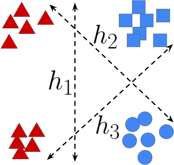
(a)

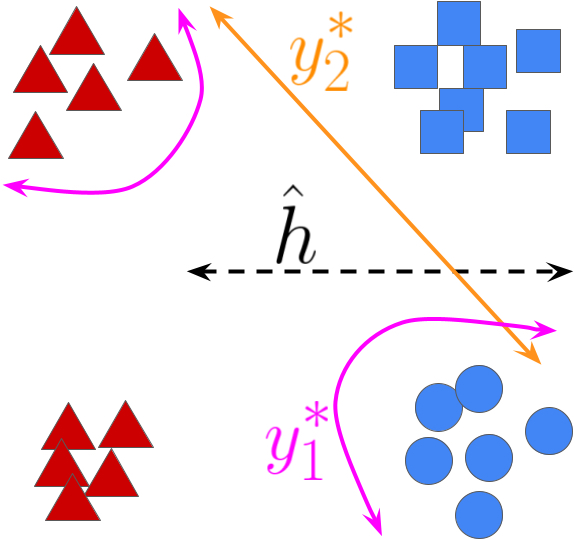
(b)

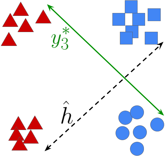
(c)

Figure 2: The advantage of Dis² over bounds based on ${\mathcal{H}}$- and ${\mathcal{H}}\Delta{\mathcal{H}}$-divergence. Consider the task of classifying circles and squares (triangles are unlabeled). (a): Because $h_{1}$ and $h_{2}\oplus h_{3}$ perfectly discriminate between ${\mathcal{S}}$ (blue) and ${\mathcal{T}}$ (red), ${\mathcal{H}}$- and ${\mathcal{H}}\Delta{\mathcal{H}}$-divergence bounds are always vacuous. In contrast, Dis² is only vacuous when 0% accuracy is induced by a reasonably likely ground truth (such as $y^{*}_{3}$ in (c), but not $y^{*}_{1}$ in (b)), and can often give non-vacuous bounds (such as $y^{*}_{2}$ in (b)).

The true labeling function is never worst-case.   More importantly, as 3.8 exemplifies, one should not expect the distribution shift to be truly worst-case, because the test distribution ${\mathcal{T}}$ and ground truth $y^{*}$ are not chosen adversarially with respect to $\hat{h}$ (Rosenfeld et al., 2022b). Figure 2 gives a simple demonstration of this point. Consider the task of learning a linear classifier to discriminate between squares and circles on the source distribution ${\mathcal{S}}$ (blue) and then bounding the error of this classifier on the target distribution ${\mathcal{T}}$ (red), whose true labels are unknown and are therefore depicted as triangles. Figure 2(a) demonstrates that both ${\mathcal{H}}$- and ${\mathcal{H}}\Delta{\mathcal{H}}$-divergence achieve their maximal value of 1, because both $h_{1}$ and $h_{2}\oplus h_{3}$ perfectly discriminate between ${\mathcal{S}}$ and ${\mathcal{T}}$. Thus both bounds would be vacuous.

Now, suppose we were to learn the max-margin $\hat{h}$ on the source distribution (Figure 2(b)). It is possible that the true labels are given by the worst-case boundary as depicted by $y^{*}_{1}$ (pink), thus “flipping” the labels and causing $\hat{h}$ to have 0 accuracy on ${\mathcal{T}}$. In this setting, a vacuous bound is correct. However, this seems rather unlikely to occur in practice—instead, recent experimental evidence (Rosenfeld et al., 2022a, Kirichenko et al., 2022, Kang et al., 2020) suggests that the true $y^{*}$ will be much simpler. The maximum disagreement discrepancy here would be approximately $0.5$, giving a test accuracy lower bound of $0.5$—this is consistent with plausible alternative labeling functions such as $y^{*}_{2}$ (orange). Even if $y^{*}$ is not linear, we may still expect that some linear function will induce larger discrepancy; this is precisely 3.3. Suppose instead we learn $\hat{h}$ as depicted in Figure 2(c). Then a simple ground truth such as $y^{*}_{3}$ (green) is plausible, which would mean $\hat{h}$ has 0 accuracy on ${\mathcal{T}}$. In this case, $y^{*}_{3}$ is also a critic with disagreement discrepancy equal to 1, and so Dis² would correctly output an error upper bound of $1$.

A setting where Dis² may be invalid.

There is one setting where it should be clear that 3.5 is less likely to be satisfied: when the representation we are using is explicitly regularized to keep $\max_{h^{\prime}\in{\mathcal{H}}}\Delta(\hat{h},h^{\prime})$ small. This occurs for domain-adversarial representation learning methods such as DANN (Ganin et al., 2016) and CDAN (Long et al., 2018), which penalize the ability to discriminate between ${\mathcal{S}}$ and ${\mathcal{T}}$ in feature space. Given a critic $h^{\prime}$ with large disagreement discrepancy, the discriminator $D(x)=\mathbf{1}\{\operatorname*{arg\,max}_{y}\hat{h}(x)_{y}=\operatorname*{arg\,max}_{y}h^{\prime}(x)_{y}\}$ will achieve high accuracy on this task (precisely, $\frac{1+\Delta(\hat{h},h^{\prime})}{2}$). By contrapositive, enforcing low discriminatory power means that the max discrepancy must also be small. It follows that for these methods Dis² should not be expected to hold universally, and in practice we see that this is the case (Figure 3). Nevertheless, when Dis² does overestimate accuracy, it does so by significantly less than prior methods.

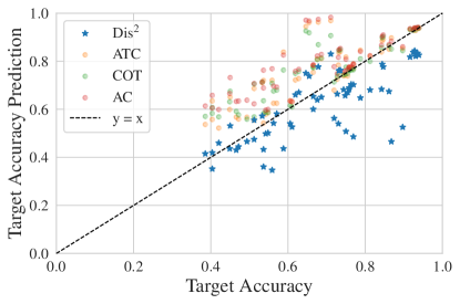
Figure 3: Dis² may be invalid when the features are explicitly learned to violate 3.5. Domain-adversarial representation learning algorithms such as DANN and CDAN indirectly minimize $\max_{h^{\prime}\in{\mathcal{H}}}\Delta(\hat{h},h^{\prime})$, meaning the necessary condition is less likely to be satisfied. Nevertheless, when Dis² does overestimate accuracy, it almost always does so by less than prior methods.

4 Efficiently Maximizing the Disagreement Discrepancy

For a classifier $\hat{h}$, Theorem 3.6 clearly prescribes how to bound its test error: first, train a critic $h^{\prime}$ on the chosen ${\mathcal{X}}$ to approximately maximize $\Delta(\hat{h},h^{\prime})$, then evaluate $\epsilon_{\hat{\mathcal{S}}}(\hat{h})$ and $\hat{\Delta}(\hat{h},h^{\prime})$ using a holdout set. The remaining difficulty is in identifying the maximizing $h^{\prime}\in{\mathcal{H}}$—that is, the one which minimizes $\epsilon_{{\mathcal{S}}}(\hat{h},h^{\prime})$ and maximizes $\epsilon_{{\mathcal{T}}}(\hat{h},h^{\prime})$. We can approximately minimize $\epsilon_{{\mathcal{S}}}(\hat{h},h^{\prime})$ by minimizing the sample average of the convex surrogate $\ell_{\textrm{logistic}}:=-\frac{1}{\log|{\mathcal{Y}}|}\log\textrm{softmax}(h(x))_{y}$ as justified by statistical learning theory. However, it is less clear how to maximize $\epsilon_{{\mathcal{T}}}(\hat{h},h^{\prime})$.

A few prior works suggest proxy losses for multiclass disagreement (Chuang et al., 2020, Pagliardini et al., 2023). We observe that these losses are not theoretically justified, as they do not upper bound the 0-1 disagreement loss we hope to minimize and are non-convex (or even concave) in the model logits. Indeed, it is easy to identify simple settings in which minimizing these losses will result in a degenerate classifier with arbitrarily small loss but high agreement. Instead, we derive a new loss which satisfies the above desiderata and thus serves as a more principled approach to maximizing disagreement.

Definition 4.1.

The disagreement logistic loss of a classifier $h$ on a labeled sample $(x,y)$ is defined as

$$\ell_{\textrm{dis}}(h,x,y) :=\frac{1}{\log 2}\log\left(1+\exp\left(h(x)_{y}-\frac{1}{|{\mathcal{Y}}|-1}\sum_{\hat{y}\neq y}h(x)_{\hat{y}}\right)\right).$$

Fact 4.2.

The disagreement logistic loss is convex in $h(x)$ and upper bounds the 0-1 disagreement loss (i.e., $\mathbf{1}\{\operatorname*{arg\,max}_{\hat{y}}h(x)_{\hat{y}}=y\}$). For binary classification, the disagreement logistic loss is equivalent to the logistic loss with the label flipped.

We expect that $\ell_{\textrm{dis}}$ can serve as a useful drop-in replacement for any future algorithm which requires maximizing disagreement in a principled manner. We combine $\ell_{\textrm{logistic}}$ and $\ell_{\textrm{dis}}$ to arrive at the empirical disagreement discrepancy objective:

$$\hat{\mathcal{L}}_{\Delta}(h^{\prime}):=\frac{1}{|\hat{\mathcal{S}}|}\sum_{x\in\hat{\mathcal{S}}}\ell_{\textrm{logistic}}(h^{\prime},x,\hat{h}(x))+\frac{1}{|\hat{\mathcal{T}}|}\sum_{x\in\hat{\mathcal{T}}}\ell_{\textrm{dis}}(h^{\prime},x,\hat{h}(x)).$$

By construction, $1-\hat{\mathcal{L}}_{\Delta}(h^{\prime})$ is concave and bounds $\hat{\Delta}(\hat{h},h^{\prime})$ from below. However, note that the representations are already optimized for accuracy on ${\mathcal{S}}$, which suggests that predictions will have low entropy and that the $\nicefrac{{1}}{{\log|{\mathcal{Y}}|}}$ scaling is unnecessary for balancing the two terms. We therefore drop the scaling factor, simply using standard cross-entropy; this often leads to higher discrepancy. In practice we optimize this objective with multiple initializations and hyperparameters and select the solution with the largest empirical discrepancy on a holdout set to ensure a conservative bound. Experimentally, we find that replacing $\ell_{\textrm{dis}}$ with either of the surrogate losses from Chuang et al. (2020), Pagliardini et al. (2023) results in smaller discrepancy; we present these results in Appendix B.

Tightening the bound by optimizing over the logits.

Looking at Theorem 3.6, it is clear that the value of the bound will decrease as the capacity of the hypothesis class is restricted. Since the number of features is large, one may expect that 3.5 holds even for a reduced feature set. In particular, it is well documented that deep networks optimized with stochastic gradient descent learn representations with small effective rank, often not much more than the number of classes (Arora et al., 2018, 2019, Pezeshki et al., 2021, Huh et al., 2022). This suggests that the logits themselves should contain most of the features’ information about ${\mathcal{S}}$ and ${\mathcal{T}}$ and that using the full feature space is unnecessarily conservative. To test this, we evaluate Dis² on the full features, the logits output by $\hat{h}$, and various fractions of the top principal components (PCs) of the features. We observe that using logits indeed results in tighter error bounds while still remaining valid—in contrast, using fewer top PCs also results in smaller error bounds, but at some point they become invalid (Figure C.2). The bounds we report in this work are thus evaluated on the logits of $\hat{h}$, except where we provide explicit comparisons in Section 5.

Identifying the ideal number of PCs via a “validity score”.

Even though reducing the feature dimensionality eventually results in an invalid bound, it is tempting to consider how we may identify approximately when this occurs, which could give a more accurate (though less conservative) prediction. We find that the optimization trajectory itself provides meaningful signal about this change. Specifically, Figure C.3 shows that for feature sets which are not overly restrictive, the critic very rapidly ascends to the maximum source agreement, then slowly begins overfitting. For much more restrictive feature sets (i.e., fewer PCs), the critic optimizes much more slowly, suggesting that we have reached the point where we are artificially restricting ${\mathcal{H}}$ and therefore underestimating the disagreement discrepancy. We design a “validity score” which captures this phenomenon, and we observe that it is roughly linearly correlated with the tightness of the eventual bound (Figure C.4). Though the score is by no means perfect, we can evaluate Dis² with successively fewer PCs and only retain those above a certain score threshold, reducing the average prediction error while remaining reasonably conservative (Figure C.5). For further details, see Appendix C.

5 Experiments

Datasets.

We conduct experiments across 11 vision benchmark datasets for distribution shift on datasets that span applications in object classification, satellite imagery, and medicine. We use four BREEDs datasets: (Santurkar et al., 2020) Entity13, Entity30, Nonliving26, and Living17; FMoW (Christie et al., 2018) and Camelyon (Bandi et al., 2018) from WILDS (Koh et al., 2021); Officehome (Venkateswara et al., 2017); Visda (Peng et al., 2018, 2017); CIFAR10, CIFAR100 (Krizhevsky and Hinton, 2009); and Domainet (Peng et al., 2019). Each of these datasets consists of multiple domains with different types of natural and synthetic shifts. We consider subpopulation shift and natural shifts induced due to differences in the data collection process of ImageNet, i.e., ImageNetv2 (Recht et al., 2019) and a combination of both. For CIFAR10 and CIFAR100 we evaluate natural shifts due to variations in replication studies (Recht et al., 2018b) and common corruptions (Hendrycks and Dietterich, 2019). For all datasets, we use the same source and target domains commonly used in previous studies (Garg et al., 2023, Sagawa et al., 2021). We provide precise details about the distribution shifts considered in Appendix A. Because distribution shifts vary widely in scope, prior evaluations which focus on only one specific type of shift (e.g., corruptions) often do not convey the full story. We therefore emphasize the need for more comprehensive evaluations across many different types of shifts and training methods, as we present here.

Experimental setup and protocols.  

Along with source-only training with ERM, we experiment with Unsupervised Domain Adaptation (UDA) methods that aim to improve target performance with unlabeled target data (FixMatch (Sohn et al., 2020), DANN Ganin et al. (2016), CDAN (Long et al., 2018), and BN-adapt (Li et al., 2016)). We experiment with Densenet121 (Huang et al., 2017) and Resnet18/Resnet50 (He et al., 2016) pretrained on ImageNet. For source-only ERM, as with other methods, we default to using strong augmentations: random horizontal flips, random crops, as well as Cutout (DeVries and Taylor, 2017) and RandAugment (Cubuk et al., 2020). Unless otherwise specified, we default to full finetuning for source-only ERM and UDA methods. We use source hold-out performance to pick the best hyperparameters for the UDA methods, since we lack labeled validation data from the target distribution. For all of these methods, we fix the algorithm-specific hyperparameters to their original recommendations following the experimental protocol in (Garg et al., 2023). For more details, see Appendix A.

Methods evaluated.

We compare Dis² to four competitive baselines: Average Confidence (AC; (Guo et al., 2017)), Difference of Confidences (DoC; (Guillory et al., 2021)), Average Thresholded Confidence (ATC; (Garg et al., 2022)), and Confidence Optimal Transport (COT; (Lu et al., 2023)). We give detailed descriptions of these methods in Appendix A. For all methods, we implement post-hoc calibration on validation source data with temperature scaling (Guo et al., 2017), which has been shown to improve performance. For Dis², we report bounds evaluated both on the full features and on the logits of $\hat{h}$ as described in Section 4. Unless specified otherwise, we set $\delta=.01$ everywhere. We also experiment with dropping the lower order concentration term in Theorem 3.6, using only the sample average. Though this is of course no longer a conservative bound, we find it is an excellent predictor of test error.

Metrics for evaluation.

We report the standard prediction metric, mean absolute error (MAE). As our emphasis is on conservative error bounds, we also report the coverage, i.e. the fraction of predictions for which the true error does not exceed the predicted error. Finally, we measure the conditional average overestimation: this is the MAE among predictions which overestimate the accuracy.

MAE $(\downarrow)$ Coverage $(\uparrow)$ Overest. $(\downarrow)$ DA? ✗ ✓ ✗ ✓ ✗ ✓ Prediction Method AC (Guo et al., 2017) 0.1055 0.1077 0.1222 0.0167 0.1178 0.1089 DoC (Guillory et al., 2021) 0.1046 0.1091 0.1667 0.0167 0.1224 0.1104 ATC NE (Garg et al., 2022) 0.0670 0.0838 0.3000 0.1833 0.0842 0.0999 COT (Lu et al., 2023) 0.0689 0.0812 0.2556 0.1833 0.0851 0.0973 Dis² (Features) 0.2807 0.1918 1.0000 1.0000 0.0000 0.0000 Dis² (Logits) 0.1504 0.0935 0.9889 0.7500 0.0011 0.0534 Dis² (Logits w/o $\delta$) 0.0829 0.0639 0.7556 0.4167 0.0724 0.0888

Table 1: Comparing the Dis² bound to prior methods for predicting accuracy. DA denotes if the representations were learned via a domain-adversarial algorithm. In addition to mean absolute error (MAE), we report what fraction of predictions correctly bound the true error (Coverage), and the average prediction error among shifts whose accuracy is overestimated (Overest.). Dis² has reasonably competitive MAE but substantially higher coverage. By dropping the concentration term in Theorem 3.6 we can do even better, at some cost to coverage.

Results.  

Reported metrics for all methods can be found in Table 1. We aggregate results over all datasets, shifts, and training methods—we stratify only by whether the training method is domain-adversarial, as this affects the validity of 3.5. We find that Dis² achieves competitive MAE while maintaining substantially higher coverage, even for domain-adversarial features. When it does overestimate accuracy, it does so by much less, implying that it is ideal for conservative estimation even when any given error bound is not technically satisfied. Dropping the concentration term performs even better (sometimes beating the baselines), at the cost of some coverage. This suggests that efforts to better estimate the true maximum discrepancy may yield even better predictors. We also show scatter plots to visualize performance on individual distribution shifts, plotting each source-target pair as a single point. For these too we report separately the results for domain-adversarial (Figure 3) and non-domain-adversarial methods (Figure 1). To avoid clutter, these two plots do not include DoC, as it performed comparably to AC. Some of the BREEDS shifts contain as few as 68 test samples, which explains why accuracy is heavily underestimated for some shifts, as the lower order term in the bound dominates at this sample size.

Figure 4(a) displays additional scatter plots which allow for a direct comparison of the variants of Dis². Finally, Figure 4(b) plots the observed violation rate (i.e. $1-$coverage) of Dis² on non-domain-adversarial methods for varying $\delta$. We observe that it lies at or below the line $y=x$, meaning the probabilistic bound provided by Theorem 3.6 holds across a range of failure probabilities. Thus we see that our probabilistic bound is empirically valid all of the time—not in the sense that each individual shift’s error is upper bounded, but rather that the desired violation rate is always satisfied.

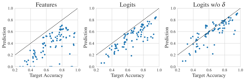
(a)

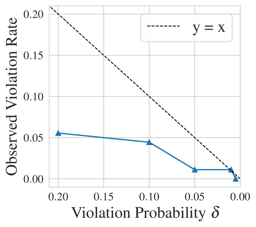
(b)

Figure 4: (a): Scatter plots depicting Dis² estimated bound vs. true error for a variety of shifts. “w/o $\delta$” indicates that the lower-order term of Theorem 3.6 has been dropped. (b): Observed bound violation rate vs. desired probability $\delta$. Observe that the true rate lies at or below $y=x$ across a range of values.

Strengthening the baselines to improve coverage.

Since the baselines we consider in this work prioritize predictive accuracy over conservative estimates, their coverage can possibly be improved without too much increase in error. We explore this option using LOOCV: for a desired coverage, we learn a parameter to either scale or shift a method’s prediction to achieve that level of coverage on all but one of the datasets. We then evaluate the method on all shifts of the remaining dataset, and we repeat this for each dataset. Appendix D reports the results for varying coverage levels. We find that (i) the baselines do not achieve the desired coverage on the held out data, though they get somewhat close; and (ii) the adjustment causes them to suffer higher MAE than Dis². Thus Dis² is on the Pareto frontier of MAE and coverage, and is preferable when conservative bounds are desirable. We believe identifying alternative methods of post-hoc prediction adjustment is a promising future direction.

6 Conclusion

The ability to evaluate trustworthy, non-vacuous error bounds for deep neural networks under distribution shift remains an extremely important open problem. Due to the wide variety of real-world shifts and the complexity of modern data, restrictive a priori assumptions on the distribution (i.e., before observing any data from the shift of interest) seem unlikely to be fruitful. On the other hand, prior methods which estimate accuracy using extra information—such as unlabeled test samples—often rely on opaque conditions whose likelihood of being satisfied is difficult to predict, and so they sometimes provide large overestimates of test accuracy with no warning signs.

This work attempts to bridge this gap with a simple, intuitive condition and a new disagreement loss which together result in competitive error prediction, while simultaneously providing an (almost) provable probabilistic error bound. We also study how the process of evaluating the bound (e.g., the optimization landscape) can provide even more useful signal, enabling better predictive accuracy. We expect there is potential to push further in each of these directions, hopefully extending the current accuracy-reliability Pareto frontier for test error bounds under distribution shift.

Appendix

Appendix A Experimental Details

A.1 Description of Baselines

Average Thresholded Confidence (ATC).   ATC first estimates a threshold $t$ on the confidence of softmax prediction (or on negative entropy) such that the number of source labeled points that get a confidence greater than $t$ match the fraction of correct examples, and then estimates the test error on on the target domain $\mathcal{D_{\mathrm{test}}}$ as the expected number of target points that obtain a score less than $t$, i.e.,

$$\text{ATC}_{\mathcal{D_{\mathrm{test}}}}(s)=\sum_{i=1}^{n}\mathbb{I}\left[s(f(x_{i}^{\prime}))<t\right]\,,$$

where $t$ satisfies: $\sum_{i=1}^{j}{\mathbb{I}\left[\max_{j\in\mathcal{Y}}(f_{j}(x_{i}))<t\right]}=\sum_{i=1}^{m}{\mathbb{I}\left[\operatorname*{arg\,max}_{j\in\mathcal{Y}}f_{j}(x_{i})\neq y_{i}\right]}$

Average Confidence (AC).   Error is estimated as the average value of the maximum softmax confidence on the target data, i.e, $\text{AC}_{\mathcal{D_{\mathrm{test}}}}=\sum_{i=1}^{n}{\max_{j\in\mathcal{Y}}f_{j}(x^{\prime}_{i})}$.

Difference Of Confidence (DOC). We estimate error on the target by subtracting the difference of confidences on source and target (as a surrogate to distributional distance (Guillory et al., 2021)) from the error on source distribution, i.e., $\text{DOC}_{\mathcal{D_{\mathrm{test}}}}=\sum_{i=1}^{n}{\max_{j\in\mathcal{Y}}f_{j}(x^{\prime}_{i})}+\sum_{i=1}^{m}{\mathbb{I}\left[\operatorname*{arg\,max}_{j\in\mathcal{Y}}f_{j}(x_{i})\neq y_{i}\right]}-\sum_{i=1}^{m}{\max_{j\in\mathcal{Y}}f_{j}(x_{i})}$. This is referred to as DOC-Feat in (Guillory et al., 2021).

Confidence Optimal Transport (COT).   COT uses the empirical estimator of the Earth Mover’s Distance between labels from the source domain and softmax outputs of samples from the target domain to provide accuracy estimates:

$$\text{COT}_{\mathcal{D_{\mathrm{test}}}}(s)=\frac{1}{2}\min_{\pi\in\Pi(S^{n},Y^{m})}\sum_{i,j=1}^{n,m}\left|\!\left|s_{i}-e_{y_{j}}\right|\!\right|_{2}\pi_{ij}\,,$$

where $S^{n}=\{f(x^{\prime}_{i})\}_{i=1}^{n}$ are the softmax outputs on the unlabeled target data and $Y^{m}=\{y_{j}\}_{j=1}^{m}$ are the labels on holdout source examples.

For all of the methods described above, we assume that $\{(x^{\prime}_{i})\}_{i=1}^{n}$ are the unlabeled target samples and $\{(x_{i},y_{i})\}_{i=1}^{m}$ are hold-out labeled source samples.

A.2 Dataset Details

In this section, we provide additional details about the datasets used in our benchmark study.

• CIFAR10 We use the original CIFAR10 dataset (Krizhevsky and Hinton, 2009) as the source dataset. For target domains, we consider (i) synthetic shifts (CIFAR10-C) due to common corruptions (Hendrycks and Dietterich, 2019); and (ii) natural distribution shift, i.e., CIFAR10v2 (Recht et al., 2018a, Torralba et al., 2008) due to differences in data collection strategy. We randomly sample 3 set of CIFAR-10-C datasets. Overall, we obtain 5 datasets (i.e., CIFAR10v1, CIFAR10v2, CIFAR10C-Frost (severity 4), CIFAR10C-Pixelate (severity 5), CIFAR10-C Saturate (severity 5)).

• CIFAR100 Similar to CIFAR10, we use the original CIFAR100 set as the source dataset. For target domains we consider synthetic shifts (CIFAR100-C) due to common corruptions. We sample 4 CIFAR100-C datasets, overall obtaining 5 domains (i.e., CIFAR100, CIFAR100C-Fog (severity 4), CIFAR100C-Motion Blur (severity 2), CIFAR100C-Contrast (severity 4), CIFAR100C-spatter (severity 2) ).

• FMoW In order to consider distribution shifts faced in the wild, we consider FMoW-WILDs (Koh et al., 2021, Christie et al., 2018) from Wilds benchmark, which contains satellite images taken in different geographical regions and at different times. We use the original train as source and OOD val and OOD test splits as target domains as they are collected over different time-period. Overall, we obtain 3 different domains.

• Camelyon17 Similar to FMoW, we consider tumor identification dataset from the wilds benchmark (Bandi et al., 2018). We use the default train as source and OOD val and OOD test splits as target domains as they are collected across different hospitals. Overall, we obtain 3 different domains.

• BREEDs We also consider BREEDs benchmark (Santurkar et al., 2020) in our setup to assess robustness to subpopulation shifts. BREEDs leverage class hierarchy in ImageNet to re-purpose original classes to be the subpopulations and defines a classification task on superclasses. We consider distribution shift due to subpopulation shift which is induced by directly making the subpopulations present in the training and test distributions disjoint. BREEDs benchmark contains 4 datasets Entity-13, Entity-30, Living-17, and Non-living-26, each focusing on different subtrees and levels in the hierarchy. We also consider natural shifts due to differences in the data collection process of ImageNet (Russakovsky et al., 2015), e.g, ImageNetv2 (Recht et al., 2019) and a combination of both. Overall, for each of the 4 BREEDs datasets (i.e., Entity-13, Entity-30, Living-17, and Non-living-26), we obtain four different domains. We refer to them as follows: BREEDsv1 sub-population 1 (sampled from ImageNetv1), BREEDsv1 sub-population 2 (sampled from ImageNetv1), BREEDsv2 sub-population 1 (sampled from ImageNetv2), BREEDsv2 sub-population 2 (sampled from ImageNetv2). For each BREEDs dataset, we use BREEDsv1 sub-population A as source and the other three as target domains.

• OfficeHome We use four domains (art, clipart, product and real) from OfficeHome dataset (Venkateswara et al., 2017). We use the product domain as source and the other domains as target.

• DomainNet We use four domains (clipart, painting, real, sketch) from the Domainnet dataset (Peng et al., 2019). We use real domain as the source and the other domains as target.

• Visda We use three domains (train, val and test) from the Visda dataset (Peng et al., 2018). While ‘train’ domain contains synthetic renditions of the objects, ‘val’ and ‘test’ domains contain real world images. To avoid confusing, the domain names with their roles as splits, we rename them as ‘synthetic’, ‘Real-1’ and ‘Real-2’. We use the synthetic (original train set) as the source domain and use the other domains as target.

Dataset Source Target CIFAR10 CIFAR10v1 CIFAR10v1, CIFAR10v2, CIFAR10C-Frost (severity 4), CIFAR10C-Pixelate (severity 5), CIFAR10-C Saturate (severity 5) CIFAR100 CIFAR100 CIFAR100, CIFAR100C-Fog (severity 4), CIFAR100C-Motion Blur (severity 2), CIFAR100C-Contrast (severity 4), CIFAR100C-spatter (severity 2) Camelyon Camelyon (Hospital 1–3) Camelyon (Hospital 1–3), Camelyon (Hospital 4), Camelyon (Hospital 5) FMoW FMoW (2002–’13) FMoW (2002–’13), FMoW (2013–’16), FMoW (2016–’18) Entity13 Entity13 (ImageNetv1 sub-population 1) Entity13 (ImageNetv1 sub-population 1), Entity13 (ImageNetv1 sub-population 2), Entity13 (ImageNetv2 sub-population 1), Entity13 (ImageNetv2 sub-population 2) Entity30 Entity30 (ImageNetv1 sub-population 1) Entity30 (ImageNetv1 sub-population 1), Entity30 (ImageNetv1 sub-population 2), Entity30 (ImageNetv2 sub-population 1), Entity30 (ImageNetv2 sub-population 2) Living17 Living17 (ImageNetv1 sub-population 1) Living17 (ImageNetv1 sub-population 1), Living17 (ImageNetv1 sub-population 2), Living17 (ImageNetv2 sub-population 1), Living17 (ImageNetv2 sub-population 2) Nonliving26 Nonliving26 (ImageNetv1 sub-population 1) Nonliving26 (ImageNetv1 sub-population 1), Nonliving26 (ImageNetv1 sub-population 2), Nonliving26 (ImageNetv2 sub-population 1), Nonliving26 (ImageNetv2 sub-population 2) Officehome Product Product, Art, ClipArt, Real DomainNet Real Real, Painiting, Sketch, ClipArt Visda Synthetic (originally referred to as train) Synthetic, Real-1 (originally referred to as val), Real-2 (originally referred to as test)

Table A.2: Details of the source and target datasets in our testbed.

A.3 Setup and Protocols

Architecture Details

For all datasets, we used the same architecture across different algorithms:

• CIFAR-10: Resnet-18 (He et al., 2016) pretrained on Imagenet

• CIFAR-100: Resnet-18 (He et al., 2016) pretrained on Imagenet

• Camelyon: Densenet-121 (Huang et al., 2017) not pretrained on Imagenet as per the suggestion made in (Koh et al., 2021)

• FMoW: Densenet-121 (Huang et al., 2017) pretrained on Imagenet

• BREEDs (Entity13, Entity30, Living17, Nonliving26): Resnet-18 (He et al., 2016) not pretrained on Imagenet as per the suggestion in (Santurkar et al., 2020). The main rationale is to avoid pre-training on the superset dataset where we are simulating sub-population shift.

• Officehome: Resnet-50 (He et al., 2016) pretrained on Imagenet

• Domainnet: Resnet-50 (He et al., 2016) pretrained on Imagenet

• Visda: Resnet-50 (He et al., 2016) pretrained on Imagenet

Except for Resnets on CIFAR datasets, we used the standard pytorch implementation (Gardner et al., 2018). For Resnet on cifar, we refer to the implementation here: https://github.com/kuangliu/pytorch-cifar. For all the architectures, whenever applicable, we add antialiasing (Zhang, 2019). We use the official library released with the paper.

For imagenet-pretrained models with standard architectures, we use the publicly available models here: https://pytorch.org/vision/stable/models.html. For imagenet-pretrained models on the reduced input size images (e.g. CIFAR-10), we train a model on Imagenet on reduced input size from scratch. We include the model with our publicly available repository.

Hyperparameter details

First, we tune learning rate and $\ell_{2}$ regularization parameter by fixing batch size for each dataset that correspond to maximum we can fit to 15GB GPU memory. We set the number of epochs for training as per the suggestions of the authors of respective benchmarks. Note that we define the number of epochs as a full pass over the labeled training source data. We summarize learning rate, batch size, number of epochs, and $\ell_{2}$ regularization parameter used in our study in Table A.3.

Dataset Epoch Batch size $\ell_{2}$ regularization Learning rate CIFAR10 50 200 0.0001 (chosen from $\{0.0001,0.001,$1e-5$,0.0\}$) 0.01 (chosen from $\{0.001,0.01,0.0001\}$) CIFAR100 50 200 0.0001 (chosen from $\{0.0001,0.001,$1e-5$,0.0\}$) 0.01 (chosen from $\{0.001,0.01,0.0001\}$) Camelyon 10 96 0.01 (chosen from $\{0.01,0.001,0.0001,0.0\}$) 0.03 (chosen from $\{0.003,0.3,0.0003,0.03\}$) FMoW 30 64 0.0 (chosen from $\{0.0001,0.001,$1e-5,0.0$\}$) 0.0001 (chosen from $\{0.001,0.01,0.0001\}$) Entity13 40 256 5e-5 (chosen from $\{$5e-5, 5e-4, 1e-4, 1e-5$\}$) 0.2 (chosen from $\{0.1,0.5,0.2,0.01,0.0\}$) Entity30 40 256 5e-5 (chosen from $\{$5e-5, 5e-4, 1e-4, 1e-5$\}$) 0.2 (chosen from $\{0.1,0.5,0.2,0.01,0.0\}$) Living17 40 256 5e-5 (chosen from $\{$5e-5, 5e-4, 1e-4, 1e-5$\}$) 0.2 (chosen from $\{0.1,0.5,0.2,0.01,0.0\}$) Nonliving26 40 256 0 5e-5 (chosen from $\{$5e-5, 5e-4, 1e-4, 1e-5$\}$) 0.2 (chosen from $\{0.1,0.5,0.2,0.01,0.0\}$) Officehome 50 96 0.0001 (chosen from $\{0.0001,0.001,$1e-5$,0.0\}$) 0.01 (chosen from $\{0.001,0.01,0.0001\}$) DomainNet 15 96 0.0001 (chosen from $\{0.0001,0.001,$1e-5$,0.0\}$) 0.01 (chosen from $\{0.001,0.01,0.0001\}$) Visda 10 96 0.0001 (chosen from $\{0.0001,0.001,$1e-5$,0.0\}$) 0.01 (chosen from $\{0.001,0.01,0.0001\}$)

Table A.3: Details of the learning rate and batch size considered in our testbed

For each algorithm, we use the hyperparameters reported in the initial papers. For domain-adversarial methods (DANN and CDANN), we refer to the suggestions made in Transfer Learning Library (Jiang et al., 2022a). We tabulate hyperparameters for each algorithm next:

• DANN, CDANN,    As per Transfer Learning Library suggestion, we use a learning rate multiplier of $0.1$ for the featurizer when initializing with a pre-trained network and $1.0$ otherwise. We default to a penalty weight of $1.0$ for all datasets with pre-trained initialization.

• FixMatch   We use the lambda is 1.0 and use threshold $\tau$ as 0.9.

Compute Infrastructure

Our experiments were performed across a combination of Nvidia T4, A6000, and V100 GPUs.

Appendix B Comparing Disagreement Losses

We define the alternate losses for maximizing disagreement:

1. Chuang et al. (2020) minimize the negative cross-entropy loss, which is concave in the model logits. That is, they add the term $\log\textrm{softmax}(h(x)_{y})$ to the objective they are minimizing. This loss results in substantially lower disagreement discrepancy than the other two.

2. Pagliardini et al. (2023) use a loss which is not too different from ours. They define the disagreement objective for a point $(x,y)$ as

   $$\log\left(1+\frac{\exp(h(x)_{y})}{\sum_{\hat{y}\neq y}\exp(h(x)_{\hat{y}})}\right).$$ (1)

For comparison, $\ell_{\textrm{dis}}$ can be rewritten as

$$\log\left(1+\frac{\exp(h(x)_{y})}{\exp\left(\frac{1}{|{\mathcal{Y}}|-1}\sum_{\hat{y}\neq y}h(x)_{\hat{y}}\right)}\right),$$ (2)

where the incorrect logits are averaged and the exponential is pushed outside the sum. This modification results in (2) being convex in the logits and an upper bound to the disagreement 0-1 loss, whereas (1) is neither.

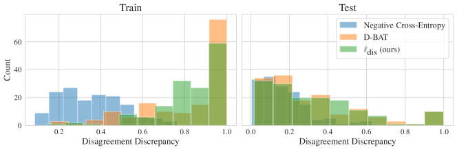
Loss	Mean Discrepancy (Train)	Mean Discrepancy (Test)
Neg. X-Ent (Chuang et al., 2020)	$0.3555\pm.0124$	$0.1694\pm.0105$
D-BAT (Pagliardini et al., 2023)	$0.8145\pm.0177$	$0.3224\pm.0212$
$\ell_{\textrm{dis}}$ (Ours)	$\underline{0.8333\pm.0132}$	$\mathbf{0.3322\pm.0205}$

Figure B.1: Histogram of disagreement discrepancies for each of the three losses, and the average values across all datasets. Bold (resp. Underline) indicates the method has higher average discrepancy under a paired t-test at significance $p=.01$ (resp. $p=.05$).

Figure B.1 displays histograms of the achieved disagreement discrepancy across all distributions for each of the disagreement losses (all hyperparameters and random seeds are the same for all three losses). The table below it reports the mean disagreement discrepancy on the train and test sets. We find that the negative cross-entropy, being a concave function, results in very low discrepancy. The loss (1) is reasonably competitive with our loss (2) on average, seemingly because it gets very high discrepancy on a subset of shifts. This suggests that it may be particularly suited for a specific type of distribution shift, though it is less good overall. Though the averages are reasonably close, the samples are not independent, so we run a paired t-test and we find that the increases to average train and test discrepancies achieved by $\ell_{\textrm{dis}}$ are significant at levels $p=0.024$ and $p=0.009$, respectively. However, with enough holdout data, a reasonable approach would be to split the data in two: one subset to validate critics trained on either of the two losses, and another to evaluate the discrepancy of whichever one is ultimately selected.

Appendix C Exploration of the Validity Score

To experiment with reducing the complexity of the class ${\mathcal{H}}$, we evaluate Dis² on progressively fewer top principal components (PCs) of the features. Precisely, for features of dimension $d$, we evaluate Dis² on the same features projected onto their top $\nicefrac{{d}}{{k}}$ components, for $k\in[1,4,16,32,64,128]$ (Figure C.2). We see that while projecting to fewer and fewer PCs does reduce the error bound value, unlike the logits it is a rather crude way to reduce complexity of ${\mathcal{H}}$, meaning at some point it goes too far and results in invalid error bounds.

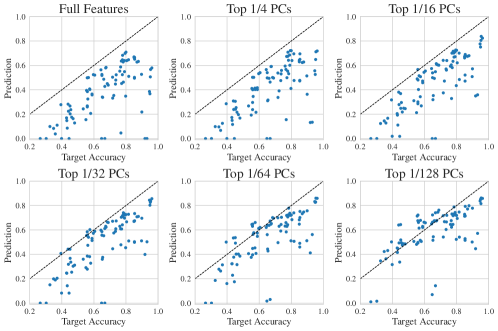
Figure C.2: Dis² bound as fewer principal components are kept. Reducing the number of top principal components crudely reduces complexity of ${\mathcal{H}}$—this leads to lower error estimates, but at some point the bounds become invalid for a large fraction of shifts.

However, during the optimization process we observe that around when this violation occurs, the task of training a critic to both agree on ${\mathcal{S}}$ and disagree on ${\mathcal{T}}$ goes from “easy” to “hard”. Figure C.3 shows that on the full features, the critic rapidly ascends to maximum agreement on ${\mathcal{S}}$, followed by slow decay (due to both overfitting and learning to simultaneously disagree on ${\mathcal{T}}$). As we drop more and more components, this optimization becomes slower.

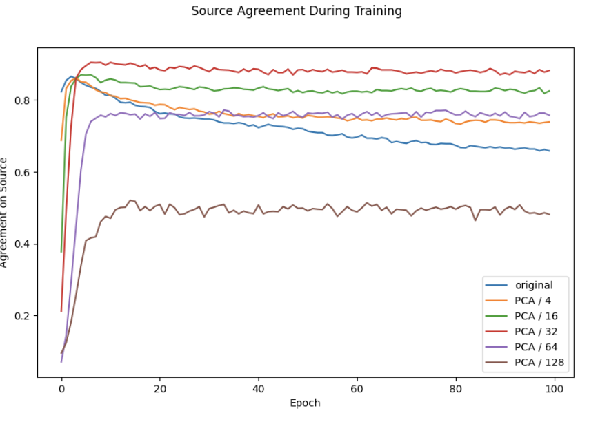
Figure C.3: Agreement on one shift between $\hat{h}$ and $h^{\prime}$ on $\hat{\mathcal{S}}$ during optimization. We observe that as the number of top PCs retained drops, the optimization occurs more slowly and less monotonically. For this particular shift, the bound becomes invalid when keeping only the top $\nicefrac{{1}}{{128}}$ components, depicted by the brown line.

We therefore design a “validity score” intended to capture this phenomenon which we refer to as the cumulative $\ell_{1}$ ratio. This is defined as the maximum agreement achieved, divided by the cumulative sum of absolute differences in agreement across all epochs up until the maximum was achieved. Formally, let $\{a_{i}\}_{i=1}^{T}$ represent the agreement between $h^{\prime}$ and $\hat{h}$ after epoch $i$, i.e. $1-\epsilon_{\hat{\mathcal{S}}}(\hat{h},h^{\prime}_{i})$, and define $m:=\operatorname*{arg\,max}_{i\in[T]}a_{i}$. The cumulative $\ell_{1}$ ratio is then $\frac{a_{m}}{a_{1}+\sum_{i=2}^{m}|a_{i}-a_{i-1}|}$. Thus, if the agreement rapidly ascends to its maximum without ever going down over the course of an epoch, this ratio will be equal to 1, and if it non-monotonically ascends then the ratio will be significantly less. This definition was simply the first metric we considered which approximately captures the behavior we observed; we expect it could be greatly improved.

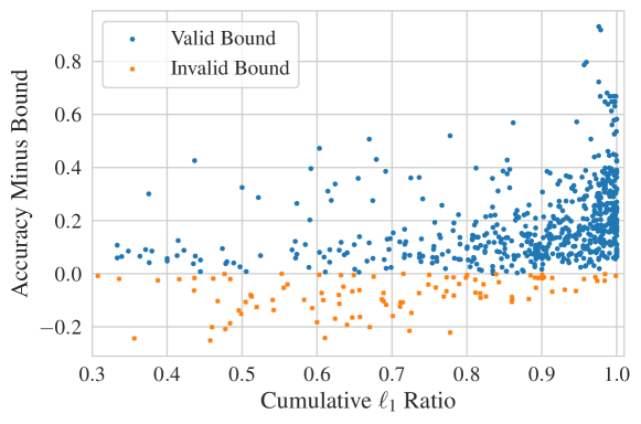
Figure C.4: Cumulative $\ell_{1}$ ratio versus error prediction gap. Despite its simplicity, the ratio captures the information encoded in the optimization trajectory, roughly linearly correlating with the tightness and validity of a given prediction. It is thus a useful metric for identifying the ideal number of top PCs to use.

Figure C.4 displays a scatter plot of the cumulative $\ell_{1}$ ratio versus the difference in estimated and true error for Dis² evaluated on the full range of top PCs. A negative value implies that we have underestimated the error (i.e., the bound is not valid). We see that even this very simply metric roughly linearly correlates with the tightness of the bound, which suggests that evaluating over a range of top PC counts and only keeping predictions whose $\ell_{1}$ ratio is above a certain threshold can improve raw predictive accuracy without reducing coverage by too much. Figure C.5 shows that this is indeed the case: compared to Dis² evaluated on the logits, keeping all predictions above a score threshold can produce more accurate error estimates, without too severely underestimating error in the worst case.

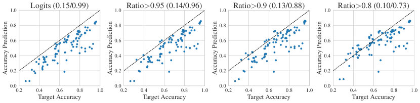
Figure C.5: Dis² bounds and MAE / coverage as the cumulative $\ell_{1}$ ratio threshold is lowered. Values in parenthesis are (MAE / coverage). By only keeping predictions with ratio above a varying threshold, we can smoothly interpolate between bound validity and raw error prediction accuracy.

Appendix D Making Baselines More Conservative with LOOCV

To more thoroughly compare Dis² to prior estimation techniques, we consider a strengthening of the baselines which may give them higher coverage without too much cost to prediction accuracy. Specifically, for each desired coverage level $\alpha\in[0.9,0.95,0.99]$, we use all but one of the datasets to learn a parameter to either scale or shift a method’s predictions enough to achieve coverage $\alpha$. We then evaluate this scaled or shifted prediction on the distribution shifts of the remaining dataset, and we repeat this for each one.

The results, found in Table D.4, demonstrate that prior methods can indeed be made to have much higher coverage, although as expected their MAE suffers. Furthermore, they still underestimate error on the tail distribution shifts by quite a bit, and they rarely achieve the desired coverage on the heldout dataset—though they usually come reasonably close. In particular, ATC (Garg et al., 2022) and COT (Lu et al., 2023) do well with a shift parameter, e.g. at the desired coverage $\alpha=0.95$ ATC matches Dis² in MAE and gets 94.4% coverage (compared to 98.9% by Dis²). However, its conditional average overestimation is quite high, almost 9%. COT gets much lower overestimation (particularly for higher coverage levels), and it also appears to suffer less on the tail distribution shifts in the sense that $\alpha=0.99$ does not induce nearly as high MAE as it does for ATC. However, at that level it only achieves 95.6% coverage, and it averages almost 5% accuracy overestimation on the shifts it does not correctly bound (compared to 0.1% by Dis²). Also, its MAE is still substantially higher than Dis², despite getting lower coverage. Finally, we evaluate the scale/shift approach on our Dis² bound without the lower order term, but based on the metrics we report there appears to be little reason to prefer it over the untransformed version, one of the baselines, or the original Dis² bound.

Taken together, these results imply that if one’s goal is predictive accuracy and tail behavior is not important (worst ~10%), ATC or COT will likely get reasonable coverage with a shift parameter—though they still significantly underestimate error on a non-negligible fraction of shifts. If one cares about the long tail of distribution shifts, or prioritizes being conservative at a slight cost to average accuracy, Dis² is clearly preferable. Finally, we observe that the randomness which determines which shifts are not correctly bounded by Dis² is “decoupled” from the distributions themselves under Theorem 3.6, in the sense that it is an artifact of the random samples, rather than a property of the distribution (recall Figure 4(b)). This is in contrast with the shift/scale approach which would produce almost identical results under larger sample sizes because it does not account for finite sample effects. This implies that some distribution shifts are simply “unsuitable” for prior methods because they do not satisfy whatever condition these methods rely on, and observing more samples will not remedy this problem. It is clear that working to understand these conditions is crucial for reliability and interpretability, since we are not currently able to identify which distributions are suitable a priori.

MAE $(\downarrow)$ Coverage $(\uparrow)$ Overest. $(\downarrow)$ $\alpha\rightarrow$ 0.9 0.95 0.99 0.9 0.95 0.99 0.9 0.95 0.99 Method Adjustment AC none 0.106 0.122 0.118 shift 0.153 0.201 0.465 0.878 0.922 0.956 0.119 0.138 0.149 scale 0.195 0.221 0.416 0.911 0.922 0.967 0.135 0.097 0.145 DoC none 0.105 0.167 0.122 shift 0.158 0.200 0.467 0.878 0.911 0.956 0.116 0.125 0.154 scale 0.195 0.223 0.417 0.900 0.944 0.967 0.123 0.139 0.139 ATC NE none 0.067 0.289 0.083 shift 0.117 0.150 0.309 0.900 0.944 0.978 0.072 0.088 0.127 scale 0.128 0.153 0.357 0.889 0.933 0.978 0.062 0.074 0.144 COT none 0.069 0.256 0.085 shift 0.115 0.140 0.232 0.878 0.944 0.956 0.049 0.065 0.048 scale 0.150 0.193 0.248 0.889 0.944 0.956 0.074 0.066 0.044 Dis² (w/o $\delta$) none 0.083 0.756 0.072 shift 0.159 0.169 0.197 0.889 0.933 0.989 0.021 0.010 0.017 scale 0.149 0.168 0.197 0.889 0.933 0.989 0.023 0.021 0.004 Dis² ($\delta=10^{-2}$) none 0.150 0.989 0.001 Dis² ($\delta=10^{-3}$) none 0.174 1.000 0.000

Table D.4: MAE, coverage, and conditional average overestimation for the strengthened baselines with a shift or scale parameter on non-domain-adversarial representations. Because a desired coverage $\alpha$ is only used when an adjustment is learned, “none”—representing no adjustment—does not vary with $\alpha$.

Appendix E Proving that 3.5 Holds

Here we describe how the equivalence of 3.5 and the bound in Theorem 3.6 allow us to prove that the assumption holds with high probability. By repeating essentially the same proof as Theorem 3.6 in the other direction, we get the following corollary:

Corollary E.1.

If 3.5 does not hold, then with probability $\geq 1-\delta$,

$$\epsilon_{\hat{\mathcal{T}}}(\hat{h}) >\epsilon_{\hat{\mathcal{S}}}(\hat{h})+\hat{\Delta}(\hat{h},h^{\prime})-\sqrt{\frac{2(n_{S}+n_{T})\log\nicefrac{{1}}{{\delta}}}{n_{S}n_{T}}}.$$

Note that the last term here is different from Theorem 3.6 because we are bounding the empirical target error, rather than the true target error. The reason for this change is that now we can make direct use of its contrapositive:

Corollary E.2.

If it is the case that

$$\epsilon_{\hat{\mathcal{T}}}(\hat{h}) \leq\epsilon_{\hat{\mathcal{S}}}(\hat{h})+\hat{\Delta}(\hat{h},h^{\prime})-\sqrt{\frac{2(n_{S}+n_{T})\log\nicefrac{{1}}{{\delta}}}{n_{S}n_{T}}},$$

then either 3.5 holds, or an event has occurred which had probability $\leq\delta$ over the randomness of the samples $\hat{\mathcal{S}},\hat{\mathcal{T}}$.

We evaluate this bound on non-domain-adversarial shifts with $\delta=10^{-6}$. As some of the BREEDS shifts have as few as 68 test samples, we restrict ourselves to shifts with $n_{T}\geq 500$ to ignore those where the finite-sample term heavily dominates; this removes a little over 20% of all shifts. Among the remainder, we find that the bound in Corollary E.2 holds 55.7% of the time when using full features and 25.7% of the time when using logits. This means that for these shifts, we can be essentially certain that 3.5—and therefore also 3.3—is true.

Note that the fact that the bound is not violated for a given shift does not at all imply that the assumption is not true. In general, the only rigorous way to prove that 3.5 does not hold would be to show that for a fixed $\delta$, the fraction of shifts for which the bound in Theorem 3.6 does not hold is larger than $\delta$ (in a manner that is statistically significant under the appropriate hypothesis test). Because this never occurs in our experiments, we cannot conclude that the assumption is ever false. At the same time, the fact that the bound does hold at least $1-\delta$ of the time does not prove that the assumption is true—it merely suggests that it is reasonable and that the bound should continue to hold in the future. This is why it is important for 3.5 to be simple and intuitive, so that we can trust that it will persist and anticipate when it will not.

However, Corollary E.2 allows us to make a substantially stronger statement. In fact, it says that for any distribution shift, with enough samples, we can prove a posteriori whether or not 3.5 holds, because the gap between these two bounds will shrink with increasing sample size.

References

- Arora et al. (2018) Sanjeev Arora, Nadav Cohen, and Elad Hazan. On the optimization of deep networks: Implicit acceleration by overparameterization. In International Conference on Machine Learning, pages 244–253. PMLR, 2018.
- Arora et al. (2019) Sanjeev Arora, Nadav Cohen, Wei Hu, and Yuping Luo. Implicit regularization in deep matrix factorization. Advances in Neural Information Processing Systems, 32, 2019.
- Baek et al. (2022) Christina Baek, Yiding Jiang, Aditi Raghunathan, and J Zico Kolter. Agreement-on-the-line: Predicting the performance of neural networks under distribution shift. In Advances in Neural Information Processing Systems, 2022.
- Bandi et al. (2018) Peter Bandi, Oscar Geessink, Quirine Manson, Marcory Van Dijk, Maschenka Balkenhol, Meyke Hermsen, Babak Ehteshami Bejnordi, Byungjae Lee, Kyunghyun Paeng, Aoxiao Zhong, et al. From detection of individual metastases to classification of lymph node status at the patient level: the camelyon17 challenge. IEEE Transactions on Medical Imaging, 2018.
- Bartlett et al. (2017) Peter L Bartlett, Dylan J Foster, and Matus J Telgarsky. Spectrally-normalized margin bounds for neural networks. In Advances in neural information processing systems, pages 6240–6249, 2017.
- Ben-David et al. (2006) Shai Ben-David, John Blitzer, Koby Crammer, and Fernando Pereira. Analysis of representations for domain adaptation. In Advances in Neural Information Processing Systems, volume 19. MIT Press, 2006.
- Ben-David et al. (2010) Shai Ben-David, John Blitzer, Koby Crammer, Alex Kulesza, Fernando Pereira, and Jennifer Wortman Vaughan. A theory of learning from different domains. Machine learning, 79:151–175, 2010.
- Chen et al. (2021a) Jiefeng Chen, Frederick Liu, Besim Avci, Xi Wu, Yingyu Liang, and Somesh Jha. Detecting errors and estimating accuracy on unlabeled data with self-training ensembles. Advances in Neural Information Processing Systems, 34:14980–14992, 2021a.
- Chen et al. (2021b) Mayee Chen, Karan Goel, Nimit S Sohoni, Fait Poms, Kayvon Fatahalian, and Christopher Ré. Mandoline: Model evaluation under distribution shift. In International Conference on Machine Learning, pages 1617–1629. PMLR, 2021b.
- Chen et al. (2022) Yining Chen, Elan Rosenfeld, Mark Sellke, Tengyu Ma, and Andrej Risteski. Iterative feature matching: Toward provable domain generalization with logarithmic environments. In Advances in Neural Information Processing Systems, volume 35, pages 1725–1736. Curran Associates, Inc., 2022.
- Christie et al. (2018) Gordon Christie, Neil Fendley, James Wilson, and Ryan Mukherjee. Functional map of the world. In Proceedings of the IEEE Conference on Computer Vision and Pattern Recognition, 2018.
- Chuang et al. (2020) Ching-Yao Chuang, Antonio Torralba, and Stefanie Jegelka. Estimating generalization under distribution shifts via domain-invariant representations. International conference on machine learning, 2020.
- Cubuk et al. (2020) Ekin D Cubuk, Barret Zoph, Jonathon Shlens, and Quoc V Le. Randaugment: Practical automated data augmentation with a reduced search space. In Proceedings of the IEEE/CVF conference on computer vision and pattern recognition workshops, pages 702–703, 2020.
- Deng and Zheng (2021) Weijian Deng and Liang Zheng. Are labels always necessary for classifier accuracy evaluation? In Proceedings of the IEEE/CVF Conference on Computer Vision and Pattern Recognition, pages 15069–15078, 2021.
- Deng et al. (2021) Weijian Deng, Stephen Gould, and Liang Zheng. What does rotation prediction tell us about classifier accuracy under varying testing environments? arXiv preprint arXiv:2106.05961, 2021.
- DeVries and Taylor (2017) Terrance DeVries and Graham W Taylor. Improved regularization of convolutional neural networks with cutout. arXiv preprint arXiv:1708.04552, 2017.
- Dziugaite and Roy (2017) Gintare Karolina Dziugaite and Daniel M Roy. Computing nonvacuous generalization bounds for deep (stochastic) neural networks with many more parameters than training data. arXiv preprint arXiv:1703.11008, 2017.
- Ganin et al. (2016) Yaroslav Ganin, Evgeniya Ustinova, Hana Ajakan, Pascal Germain, Hugo Larochelle, François Laviolette, Mario Marchand, and Victor Lempitsky. Domain-adversarial training of neural networks. J. Mach. Learn. Res., 17(1):2096–2030, jan 2016. ISSN 1532-4435.
- Gardner et al. (2018) Jacob Gardner, Geoff Pleiss, Kilian Q Weinberger, David Bindel, and Andrew G Wilson. Gpytorch: Blackbox matrix-matrix gaussian process inference with gpu acceleration. In Advances in Neural Information Processing Systems, pages 7576–7586, 2018.
- Garg et al. (2021) Saurabh Garg, Sivaraman Balakrishnan, J Zico Kolter, and Zachary C Lipton. Ratt: Leveraging unlabeled data to guarantee generalization. arXiv preprint arXiv:2105.00303, 2021.
- Garg et al. (2022) Saurabh Garg, Sivaraman Balakrishnan, Zachary Chase Lipton, Behnam Neyshabur, and Hanie Sedghi. Leveraging unlabeled data to predict out-of-distribution performance. In International Conference on Learning Representations, 2022.
- Garg et al. (2023) Saurabh Garg, Nick Erickson, James Sharpnack, Alex Smola, Siva Balakrishnan, and Zachary Lipton. Rlsbench: A large-scale empirical study of domain adaptation under relaxed label shift. In International Conference on Machine Learning (ICML), 2023.
- Guillory et al. (2021) Devin Guillory, Vaishaal Shankar, Sayna Ebrahimi, Trevor Darrell, and Ludwig Schmidt. Predicting with confidence on unseen distributions. arXiv preprint arXiv:2107.03315, 2021.
- Guo et al. (2017) Chuan Guo, Geoff Pleiss, Yu Sun, and Kilian Q Weinberger. On calibration of modern neural networks. In International Conference on Machine Learning (ICML), 2017.
- He et al. (2016) Kaiming He, Xiangyu Zhang, Shaoqing Ren, and Jian Sun. Deep Residual Learning for Image Recognition. In Computer Vision and Pattern Recognition (CVPR), 2016.
- Hendrycks and Dietterich (2019) Dan Hendrycks and Thomas Dietterich. Benchmarking neural network robustness to common corruptions and perturbations. arXiv preprint arXiv:1903.12261, 2019.
- Huang et al. (2017) Gao Huang, Zhuang Liu, Laurens Van Der Maaten, and Kilian Q Weinberger. Densely connected convolutional networks. In Proceedings of the IEEE conference on computer vision and pattern recognition, pages 4700–4708, 2017.
- Huh et al. (2022) Minyoung Huh, Hossein Mobahi, Richard Zhang, Brian Cheung, Pulkit Agrawal, and Phillip Isola. The low-rank simplicity bias in deep networks, 2022. URL https://openreview.net/forum?id=dn4B7Mes2z.
- Hume (2000) David Hume. An enquiry concerning human understanding: A critical edition, volume 3. Oxford University Press on Demand, 2000.
- Jiang et al. (2022a) Junguang Jiang, Yang Shu, Jianmin Wang, and Mingsheng Long. Transferability in deep learning: A survey, 2022a.
- Jiang et al. (2022b) Yiding Jiang, Vaishnavh Nagarajan, Christina Baek, and J Zico Kolter. Assessing generalization of SGD via disagreement. In International Conference on Learning Representations, 2022b.
- Kang et al. (2020) Bingyi Kang, Saining Xie, Marcus Rohrbach, Zhicheng Yan, Albert Gordo, Jiashi Feng, and Yannis Kalantidis. Decoupling representation and classifier for long-tailed recognition. In International Conference on Learning Representations, 2020.
- Kirichenko et al. (2022) Polina Kirichenko, Pavel Izmailov, and Andrew Gordon Wilson. Last layer re-training is sufficient for robustness to spurious correlations. arXiv preprint arXiv:2204.02937, 2022.
- Koh et al. (2021) Pang Wei Koh, Shiori Sagawa, Henrik Marklund, Sang Michael Xie, Marvin Zhang, Akshay Balsubramani, Weihua Hu, Michihiro Yasunaga, Richard Lanas Phillips, Irena Gao, Tony Lee, Etienne David, Ian Stavness, Wei Guo, Berton A. Earnshaw, Imran S. Haque, Sara Beery, Jure Leskovec, Anshul Kundaje, Emma Pierson, Sergey Levine, Chelsea Finn, and Percy Liang. WILDS: A benchmark of in-the-wild distribution shifts. In International Conference on Machine Learning (ICML), 2021.
- Krizhevsky and Hinton (2009) Alex Krizhevsky and Geoffrey Hinton. Learning Multiple Layers of Features from Tiny Images. Technical report, Citeseer, 2009.
- Li et al. (2016) Yanghao Li, Naiyan Wang, Jianping Shi, Jiaying Liu, and Xiaodi Hou. Revisiting batch normalization for practical domain adaptation. arXiv preprint arXiv:1603.04779, 2016.
- Long et al. (2018) Mingsheng Long, Zhangjie Cao, Jianmin Wang, and Michael I Jordan. Conditional adversarial domain adaptation. Advances in neural information processing systems, 31, 2018.
- Long and Sedghi (2019) Philip M Long and Hanie Sedghi. Generalization bounds for deep convolutional neural networks. arXiv preprint arXiv:1905.12600, 2019.
- Lu et al. (2023) Yuzhe Lu, Zhenlin Wang, Runtian Zhai, Soheil Kolouri, Joseph Campbell, and Katia Sycara. Predicting out-of-distribution error with confidence optimal transport. In ICLR 2023 Workshop on Pitfalls of limited data and computation for Trustworthy ML, 2023.
- Mansour et al. (2009) Yishay Mansour, Mehryar Mohri, and Afshin Rostamizadeh. Domain adaptation: Learning bounds and algorithms. arXiv preprint arXiv:0902.3430, 2009.
- Nagarajan and Kolter (2019a) Vaishnavh Nagarajan and J Zico Kolter. Deterministic pac-bayesian generalization bounds for deep networks via generalizing noise-resilience. arXiv preprint arXiv:1905.13344, 2019a.
- Nagarajan and Kolter (2019b) Vaishnavh Nagarajan and J. Zico Kolter. Uniform convergence may be unable to explain generalization in deep learning. In Advances in Neural Information Processing Systems, volume 32. Curran Associates, Inc., 2019b.
- Nakkiran and Bansal (2019) Preetum Nakkiran and Yamini Bansal. Distributional generalization: A new kind of generalization. ArXiv, abs/2009.08092, 2019.
- Neyshabur (2017) Behnam Neyshabur. Implicit regularization in deep learning. arXiv preprint arXiv:1709.01953, 2017.
- Neyshabur et al. (2015) Behnam Neyshabur, Ryota Tomioka, and Nathan Srebro. Norm-based capacity control in neural networks. In Conference on Learning Theory, pages 1376–1401, 2015.
- Neyshabur et al. (2017) Behnam Neyshabur, Srinadh Bhojanapalli, David McAllester, and Nathan Srebro. Exploring generalization in deep learning. arXiv preprint arXiv:1706.08947, 2017.
- Neyshabur et al. (2018) Behnam Neyshabur, Zhiyuan Li, Srinadh Bhojanapalli, Yann LeCun, and Nathan Srebro. The role of over-parametrization in generalization of neural networks. In International Conference on Learning Representations, 2018.
- Ovadia et al. (2019) Yaniv Ovadia, Emily Fertig, Jie Ren, Zachary Nado, David Sculley, Sebastian Nowozin, Joshua V Dillon, Balaji Lakshminarayanan, and Jasper Snoek. Can you trust your model’s uncertainty? evaluating predictive uncertainty under dataset shift. arXiv preprint arXiv:1906.02530, 2019.
- Pagliardini et al. (2023) Matteo Pagliardini, Martin Jaggi, François Fleuret, and Sai Praneeth Karimireddy. Agree to disagree: Diversity through disagreement for better transferability. In The Eleventh International Conference on Learning Representations, 2023.
- Peng et al. (2017) Xingchao Peng, Ben Usman, Neela Kaushik, Judy Hoffman, Dequan Wang, and Kate Saenko. Visda: The visual domain adaptation challenge, 2017.
- Peng et al. (2018) Xingchao Peng, Ben Usman, Kuniaki Saito, Neela Kaushik, Judy Hoffman, and Kate Saenko. Syn2real: A new benchmark forsynthetic-to-real visual domain adaptation. arXiv preprint arXiv:1806.09755, 2018.
- Peng et al. (2019) Xingchao Peng, Qinxun Bai, Xide Xia, Zijun Huang, Kate Saenko, and Bo Wang. Moment matching for multi-source domain adaptation. In Proceedings of the IEEE/CVF international conference on computer vision, pages 1406–1415, 2019.
- Pezeshki et al. (2021) Mohammad Pezeshki, Oumar Kaba, Yoshua Bengio, Aaron C Courville, Doina Precup, and Guillaume Lajoie. Gradient starvation: A learning proclivity in neural networks. Advances in Neural Information Processing Systems, 34:1256–1272, 2021.
- Platanios et al. (2017) Emmanouil A Platanios, Hoifung Poon, Tom M Mitchell, and Eric Horvitz. Estimating accuracy from unlabeled data: A probabilistic logic approach. arXiv preprint arXiv:1705.07086, 2017.
- Platanios et al. (2016) Emmanouil Antonios Platanios, Avinava Dubey, and Tom Mitchell. Estimating accuracy from unlabeled data: A bayesian approach. In International Conference on Machine Learning, pages 1416–1425. PMLR, 2016.
- Rahimian and Mehrotra (2019) Hamed Rahimian and Sanjay Mehrotra. Distributionally robust optimization: A review. arXiv preprint arXiv:1908.05659, 2019.
- Recht et al. (2018a) Benjamin Recht, Rebecca Roelofs, Ludwig Schmidt, and Vaishaal Shankar. Do cifar-10 classifiers generalize to cifar-10? arXiv preprint arXiv:1806.00451, 2018a.
- Recht et al. (2018b) Benjamin Recht, Rebecca Roelofs, Ludwig Schmidt, and Vaishaal Shankar. Do cifar-10 classifiers generalize to cifar-10? 2018b. https://arxiv.org/abs/1806.00451.
- Recht et al. (2019) Benjamin Recht, Rebecca Roelofs, Ludwig Schmidt, and Vaishaal Shankar. Do imagenet classifiers generalize to imagenet? In International Conference on Machine Learning, pages 5389–5400. PMLR, 2019.
- Rosenfeld et al. (2021) Elan Rosenfeld, Pradeep Kumar Ravikumar, and Andrej Risteski. The risks of invariant risk minimization. In International Conference on Learning Representations, 2021.
- Rosenfeld et al. (2022a) Elan Rosenfeld, Pradeep Ravikumar, and Andrej Risteski. Domain-adjusted regression or: Erm may already learn features sufficient for out-of-distribution generalization. arXiv preprint arXiv:2202.06856, 2022a.
- Rosenfeld et al. (2022b) Elan Rosenfeld, Pradeep Ravikumar, and Andrej Risteski. An online learning approach to interpolation and extrapolation in domain generalization. In Proceedings of The 25th International Conference on Artificial Intelligence and Statistics, volume 151 of Proceedings of Machine Learning Research, pages 2641–2657. PMLR, 28–30 Mar 2022b.
- Russakovsky et al. (2015) Olga Russakovsky, Jia Deng, Hao Su, Jonathan Krause, Sanjeev Satheesh, Sean Ma, Zhiheng Huang, Andrej Karpathy, Aditya Khosla, Michael Bernstein, et al. Imagenet large scale visual recognition challenge. International journal of computer vision, 115(3):211–252, 2015.
- Sagawa et al. (2021) Shiori Sagawa, Pang Wei Koh, Tony Lee, Irena Gao, Sang Michael Xie, Kendrick Shen, Ananya Kumar, Weihua Hu, Michihiro Yasunaga, Henrik Marklund, Sara Beery, Etienne David, Ian Stavness, Wei Guo, Jure Leskovec, Kate Saenko, Tatsunori Hashimoto, Sergey Levine, Chelsea Finn, and Percy Liang. Extending the wilds benchmark for unsupervised adaptation. In NeurIPS Workshop on Distribution Shifts, 2021.
- Santurkar et al. (2020) Shibani Santurkar, Dimitris Tsipras, and Aleksander Madry. Breeds: Benchmarks for subpopulation shift. arXiv preprint arXiv:2008.04859, 2020.
- Sohn et al. (2020) Kihyuk Sohn, David Berthelot, Nicholas Carlini, Zizhao Zhang, Han Zhang, Colin A Raffel, Ekin Dogus Cubuk, Alexey Kurakin, and Chun-Liang Li. Fixmatch: Simplifying semi-supervised learning with consistency and confidence. Advances in Neural Information Processing Systems, 33, 2020.
- Sun et al. (2016) Baochen Sun, Jiashi Feng, and Kate Saenko. Return of frustratingly easy domain adaptation. In Proceedings of the AAAI Conference on Artificial Intelligence, 2016.
- Torralba et al. (2008) Antonio Torralba, Rob Fergus, and William T. Freeman. 80 million tiny images: A large data set for nonparametric object and scene recognition. IEEE Transactions on Pattern Analysis and Machine Intelligence, 30(11):1958–1970, 2008.
- Venkateswara et al. (2017) Hemanth Venkateswara, Jose Eusebio, Shayok Chakraborty, and Sethuraman Panchanathan. Deep hashing network for unsupervised domain adaptation. In Proceedings of the IEEE Conference on Computer Vision and Pattern Recognition, pages 5018–5027, 2017.
- Zhang et al. (2016) Chiyuan Zhang, Samy Bengio, Moritz Hardt, Benjamin Recht, and Oriol Vinyals. Understanding deep learning requires rethinking generalization. arXiv preprint arXiv:1611.03530, 2016.
- Zhang (2019) Richard Zhang. Making convolutional networks shift-invariant again. In ICML, 2019.
- Zhang et al. (2019) Yuchen Zhang, Tianle Liu, Mingsheng Long, and Michael Jordan. Bridging theory and algorithm for domain adaptation. In International Conference on Machine Learning. PMLR, 2019.
- Zhou et al. (2018) Wenda Zhou, Victor Veitch, Morgane Austern, Ryan P Adams, and Peter Orbanz. Non-vacuous generalization bounds at the imagenet scale: a pac-bayesian compression approach. arXiv preprint arXiv:1804.05862, 2018.