Prompt Algebra for Task Composition

Abstract

We investigate whether prompts learned independently for different tasks can be later combined through prompt algebra to obtain a model that supports composition of tasks. We consider Visual Language Models (VLM) with prompt tuning as our base classifier and formally define the notion of prompt algebra. We propose constrained prompt tuning to improve performance of the composite classifier. In the proposed scheme, prompts are constrained to appear in the lower dimensional subspace spanned by the basis vectors of the pre-trained vocabulary. Further regularization is added to ensure that the learned prompt is grounded correctly to the existing pre-trained vocabulary. We demonstrate the effectiveness of our method on object classification and object-attribute classification datasets. On average, our composite model obtains classification accuracy within 2.5% of the best base model. On UTZappos it improves classification accuracy over the best base model by 8.45% on average.

1 Introduction

Recent works have shown that pre-trained text tokens respect compositional relationships in the text feature space between entities [22, 32, 7]. For example, a text feature of Queen can be obtained by adding the residual text feature of woman-man to the text feature of King as shown in Figure 1 (a). On the other hand, the prompt-tuning literature [15, 17, 18, 19] suggests that usage of soft-prompt tokens to prompt a model can result in powerful classifiers that are on par with the classification ability of fine-tuned models.

In this paper, we raise the question: are soft-prompt tokens compositional? Is it possible to combine two prompt-tokens that are trained independently on separate classification tasks to obtain a composite classifier (Figure 1b)? In our experiments, we provide evidence that such a relationship exists. We empirically show that prompt tokens can be manipulated using prompt algebra to obtain classifiers for composite tasks.

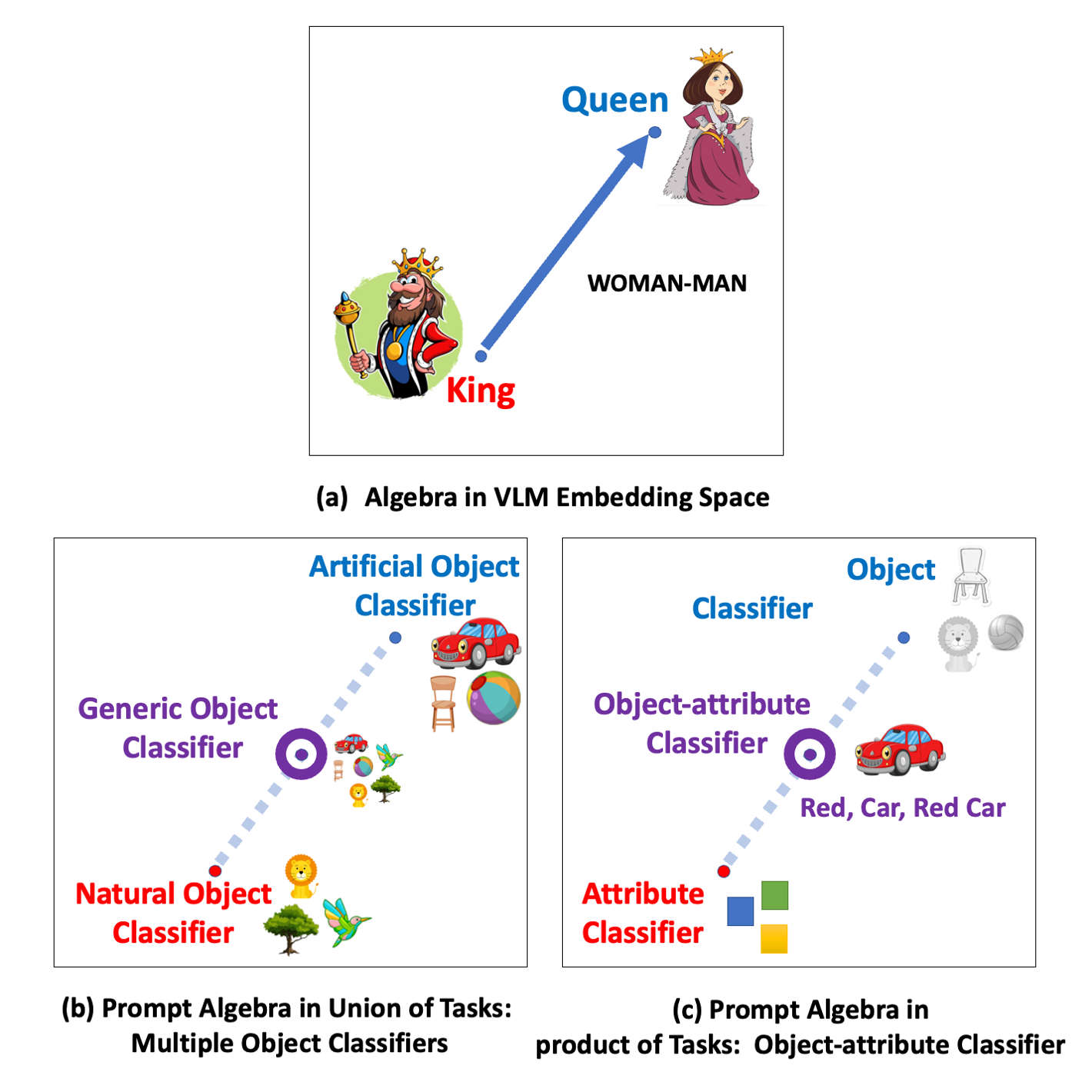
Figure 1: Overview of prompt algebra. (a) VLM models exhibit compositionality between entities in the text feature space. (b) Prompt algebra can be used to combine prompts obtained from natural object classification and artificial object classification to produce prompts that result in a generic object classifier. (c) Combining attribute and object classifiers results in a prompt that performs well in object, attribute and object-attribute classification tasks.

This observation is important to the machine learning community for a simple reason. Recent advancements in deep learning[8, 39, 5] have paved the path for models with very competitive performance in specific downstream classification tasks. However, these models require annotated data for every class and have very limited flexibility to adapt to new tasks without retraining. Task composition enables composing two or more base classifiers to support classification in the full product space of classes avoiding the combinatorial explosion of classes. In general there are two forms of task compositionality that we are interested in:

Union of Tasks. When two classifiers $C_{1}$ and $C_{2}$ are trained independently on two separate tasks (natural object classification and artificial object recognition respectively) as shown in Figure 2(a), the resulting classifier should be able to perform classification across all classes that were supported in the base classifier (both natural and artificial objects). In Figure 1(b), we illustrate how prompt algebra functions in this specific use case. We interpolate prompts learned for natural object classification and artificial object classification to arrive at a prompt that performs classification across both natural and artificial objects.

Product of tasks. If new object classes can be defined by composing classes of base classifiers together, the resulting classifier should perform well on these composite classes. This situation arises when there exits two interpretations (in terms of annotation) for a given image. For the remainder of this paper, we refer such data as multi-view data; where each view refers to a unique interpretation. For an example, in Figure 2(b), base classifiers are an object classifier and an attribute classifier. It is possible to define new classes by considering the product space of object and attribute classes. For example, young cat is a composition of the concepts of young attribute and cat object. The resulting classifier should be able to recognize such composite concepts in addition to concepts supported by base classifiers. Prompt algebra can be used to generate a prompt (by interpolating base prompts) that recognizes objects, attributes and object-attribute pairs as shown in In Figure 1(c).

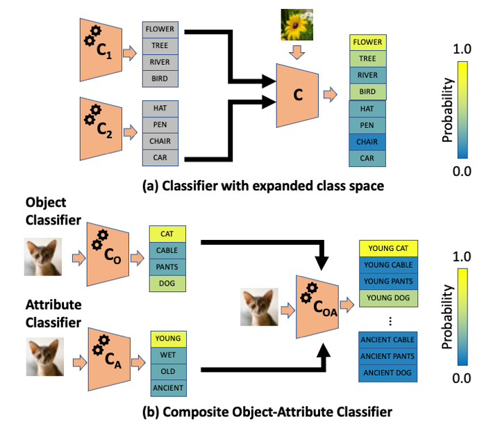
Figure 2: Desired properties of a composed classifier. (a) The composed classifier should support the union of the classes supported by independently trained base classifiers. (b) When classes of base classifiers (e.g., object classes and attribute classes) can be composed to form new composite classes (attribute-object classes), the composed classifier should support these composite classes as well.

In this paper, we propose to select a prompt from the convex hull of base prompts using a prompt algebraic operation to support task compositionality. We argue that prompts should have a common grounding for them to gracefully compose and prevent any destructive interference. We encourage this property by constraining prompts to lie in a common subspace and introducing regularization to ensure that pre-existing relationships in the pretrained vocabulary are preserved. We make following contributions in this paper:

1. We show that independently learned classifier models can be integrated together using prompt algebra to support both union of task and product of task compositionality.

2. We propose a constrained prompt generation method based on loss regularization to improve performance of the composed classifier.

2 Related Work

Vision Language Models. Recent works in both vision and language communities have explored the possibility of learning a joint vision-language embedding to support multi-modal tasks. Following the success of large language models [4, 20, 28], earlier attempts have tried to reuse the structure of language models (such as BERT) to learn a joint embedding. VL-BERT[31] used faster R-CNN based object proposals to generate image tokens and combined them together with word tokens to learn a joint representation. On the other hand, VILBERT [21] used two separate language and vision towers to first obtain image and text features and then used a co-attention network to fuse features together. Most of later works adopted this strategy for learning. CLIP [27] model optimized parameters of vision and language towers using a contrastive loss in the feature space. ALBEF model [16] added a secondary fusion network on top of vision-language features and used momentum distillation to learn representations. More recent works have used noisy-annotated data[27] and web-crawled data [1] to create powerful models that generalize well. These models have demonstrated strong zero-shot and few-shot recognition ability in multiple language-vision tasks[27, 1, 10].
Prompt Tuning. Prompt tuning was first introduced in the NLP community to perform zero-shot inference with pretrained models . A text prompt, in the traditional sense, is a set of words that describes the task desired from a network. This is now widely used with in-context-learning in NLP [2, 3]. It was later discovered that different prompts that are semantically similar can yield varying performance on ML tasks. Prompt engineering attempted to find the best prompt that produces optimum performance in a downstream task. However, it is both time and resource consuming as the optimization cannot be automated. Soft-prompt tuning [19, 17, 35] attempts to replace prompt tuning with an optimization framework. Soft prompting optimizes over vectors in the word embedding space to find a set of representations that improves performance of the downstream task. It was later shown that prompting can be done even at a deeper level in a network to obtain better downstream task performance [18]. Several recent works have explored using soft prompt tuning in several NLP and vision tasks [11].
Product of Task Compositionality. Several recent works have studied product of task compositionally in deep learning models. Given a multi-view dataset where each view is described by a finite set of classes, two views can be composed together to form a composite class. Object-attribute datasets have been commonly used to study the task compositionally of models. In this setting, objects and attributes serve as alternating views of the same image and the product space defined by {attributes, objects} becomes the composite-class space. Previous works have used transformation functions [23, 14], late fusion networks[26] and graph neural networks [30, 24] to obtain better task compositionally. Recently, it was shown that prompt tuning with class specific prompts can obtain promising results in this task [25]. However, in all these methods, both views of the dataset is shown simultaneously to the learned classifier during training. In contrast, in this paper, we study the special case when two classifiers are trained on each view independently with partial annotation.
Continual Learning. Continual learning is a learning paradigm where a single model is required a learn a series of tasks sequentially [33, 29, 6]. There exists three flavors of continual learning [34], namely task incremental learning, domain incremental learning and class incremental learning (CIL). The setting we explore in this paper is similar in spirit to CIL with a notable difference: CIL typically involves retraining an existing model with data belonging to the new tasks (and possibly with replays from previous tasks) with the objective of performing well across union of tasks. In contrast, we explore ways to expand task support by combining two independently trained classifiers on sub-tasks.

3 Background

3.1 Multi-class Classification with VLM

Recent advances in VLM have resulted in models with better zero-shot classification capabilities [27, 16, 10, 1]. In this paper we limit our discussion to VLM models with separate vision and language towers. Let us consider such a network as illustrated in Figure 3. This network contains a vision encoder $e_{v}$ and a text encoder $e_{t}$. Such a pretrained network can be used to perform $c$ way classification.

Given a image $I$, first the vision tower is used to extract the vision feature $e_{v}(I)$. Then, class specific text feature $e_{t}(t_{i})$ is calculated for a text of the form $t_{i}=[t_{common},c_{i}]$, where $t_{common}$ is a class-agnostic prompt and $c_{i}$ is a class specific prompt for $i^{\text{th}}$ class. In our experiments we use class agnostic prompt $t_{common}$ to be the text ”Image of a ”. Class labels are used as class specific prompts $c_{i}$. Finally, the distance $d$ between the image feature $e_{v}(I)$ and text features $e_{t}(t_{i})$ are calculated. Cosine-distance is commonly used as the distance metric. During training, the pretrained model is finetuned by considering image-text distance $d$ to be the class logit score and minimizing cross-entropy loss.

During inference, the class that produces lowest image-text feature distance $\arg\min_{i}d(e_{v}(I),e_{t}(t_{i}))$ is considered to be the model prediction. Zero-shot classification is trivial within this framework. A classifier can be converted into a zero-shot classifier by simply extending the list of prompts passed to the text encoder, by including zero-shot class labels.

3.2 Prompt Tuning

Prompt Tuning is a recent advancement in Machine Learning [15] that allows output of a transformer based model to be influenced by a learnable set of token embeddings. A text-prompt of the form $t_{i}=[t_{common},c_{i}]$ is extended to the form $t_{i}^{\prime}=[t_{common},v,c_{i}]$ by introducing a nominal token $v$. During training, embedding vector of the nominal token $e_{t}(v)$ is optimized with the aim of minimizing the model objective function. Prompt tuning is more parameter efficient, yet produces comparable performance to finetuning in various language and vision tasks [19]. Once trained, the prompt $v$ encodes information about the downstream task. For the remainder of the paper we refer to $v$ as the task prompt.

A prompt-tuned VLM can be used for multi-class classification as shown in Figure 3. The only difference from before is the incorporation of prompts when producing input to the text encoder (see the yellow colored input in Figure 3). In this setup, text features are calculated for a set of prompts $t_{i}=[t_{common},v,c_{i}]$, where $v$ is the learned soft prompt.

Figure 3: Overview of VLM based classification. Image is passed through the vision encoder $e_{v}$ to obtain image features. In finetuning, text prompts (in blue) are passed to the language encoder $e_{t}$ to get text features. Distance between Image features and text features is used to optimize parameters of $e_{t}$ and $e_{v}$ using a contrastive loss. In prompt tunning, text input (in yellow) is appended with a special token $v$. During training, all parameters except token embeddings of $v$ is kept fixed. Token embeddings of $v$ are optimized with respect to the contrastive loss same as before.

4 Composing Independent Classifiers

In this section, we describe our proposed solution for composing independently learned classifiers. First, we describe our choice of model backbone followed by details of prompt algebra. We end this section by introducing constrained prompt learning that encourages representations to have desired properties for prompt algebra.

4.1 Model Architecture

We use a VLM equipped with prompt-tuning as our choice of model due to several reasons. VLM training and inference is free of class-specific layers. This enables easy integration of models trained on different tasks. A prompt is added as a part of the input to the network. Compared to other approaches that generate task specific architectural changes [37], prompt tuning allows a direct way to manipulate model parameters by transforming prompts. For each task $j$, we train a class-agnostic prompt $v_{j}$ to maximize model performance with respect to a given dataset. Specifically, for classification tasks, a text input to the text encoder is formed as $t_{i}=[t_{common},v_{j},c_{i}]$. During training, parameter $v_{j}$ is optimized by minimizing cross-entropy loss.

4.2 Prompt Algebra

Let $\mathbf{v}=[v_{0},v_{1},\dots]$ be a set of prompts trained on a collection of datasets. The goal of prompt algebra is to create prompts for new tasks by linearly combining the prompts $v_{i}$. That is, prompt algebra defines a linear transformation $f(\mathbf{v})=\sum\theta_{i}v_{i}\forall\theta_{i}\geq 0$.

Pretrained language models and Vision-Language Models (VLM) exhibit properties of compositionality in the vocabulary space. In prompt tuning, a special token $v_{j}$ is learned for task $j$. Once trained, the special token $v_{j}$ modulates class label $c_{i}$ such that the prompt $t_{i}=[t_{common},v_{j},c_{i}]$ produces highest correlation with image from class $i$ compared to images from other classes. In this paper, we claim that soft prompts trained this way exhibit the same compositionality property their word-token counter part process. i.e. if $e_{t}[v_{A}]$ and $e_{t}[v_{B}]$ are prompt embeddings learned for two tasks taskA and taskB, the prompt algebraic operation $\theta_{A}\cdot e_{t}[v_{A}]+\theta_{B}\cdot e_{t}[v_{B}]$ results in a modulation that align images with labels of both tasks A and B (here, $\theta_{A},\theta_{B}$ are constant weights). We use this property to compose independently trained prompt-tuning based classifiers. Prompts of the composite model are obtained by $\sum_{j}\theta_{j}v_{j}$, where, $\theta_{j}$ is a weight associated with each task.

4.3 Constrained Prompt Tuning.

In Section 5, we empirically show that prompt algebra is effective for prompts trained on certain datasets without any additional conditioning. However, this is not guaranteed to occur in every scenario due to multiple reasons. When task prompts are trained independently from each other, it’s possible for prompts to appear in very different sub-spaces. There is also a possibility that prompts may interfere with each other as well as with other vocabulary tokens when this is the case. To avoid the former problem, we propose constraining prompt space to the lower dimensional subspace of the pre-trained vocabulary.

For the latter problem, we note that when VLMs soft prompts are trained on a downstream task, the prompt learns to attend to the task’s labels of known classes. However, learned prompts have no incentive in learning a non-degenerate attention mechanism that will generalize well to unseen labels or contexts. Although this behaviour is acceptable when fine-tuning on a specific task, it may produce undesirable effects when prompts are combined and reused on new tasks. As a counter measure, we wish to regularize the learning to better ground the prompts in the pre-trained vocabulary tokens. This encourages the otimization to move along more meaningful subspaces and to learn more robust attention mechanisms. In this paper, we explore two forms of regularizations: multi-view regularization and class-agnostic regularization.

Constraining prompt space. In order to encourage compositionality, we aim to force prompts to reside in a common sub-space. We choose the lower dimensional subspace of the pre-trained vocabulary as our choice of the sub-space as it’s a static reference. On the other hand, tokens in this space themselves are composible. Therefore, by making this choice, we hope soft prompts will gracefully compose with other vocabulary tokens as well.

Specifically, given the pretrained vocabulary $V$, we find the eigendecomposition of the co-relation matrix $V^{T}V$, and form a projection matrix $E$ using the eigenvectors of $V^{T}V$ that corresponds to largest $m$ eigenvalues. We compute $m$ in order to preserve a desired amount of spectral energy (90% in our experiments). During both training and inference, each prompt token $v_{j}$ is projected to the lower dimensional subspace of $V$ using the projection operation $Pv_{j}$. The composite prompt vector now becomes $f(\mathbf{v})=P\sum_{i}\theta_{i}\cdot v_{i}$. In this process, the eigen decomposition happens only at the beginning of training. Therefore the additional processing overhead is fixed.

Multi-view Regularization. Multi-view regularization is a specialized regularization that can be applied when data has multiple views, i.e., when samples in the dataset have multiple annotations. For example, an image could be annotated both with an object category (e.g., cat) and an attribute (e.g., old). Let $\mathcal{Y}^{A}$ and $\mathcal{Y}^{B}$ be the label space corresponding to to possible views in the dataset. For an example, $\mathcal{Y}^{A}$ may be object labels and $\mathcal{Y}^{B}$ may be attribute annotations. Suppose we are training a classifier on $\mathcal{Y}^{A}$. We use the following regularization procedure (outlined in Figure 4):

1. Let $(I,y^{A}_{i})$ be an image-label pair from view A, for example $y^{A}_{i}=\texttt{cat}$. Let $\mathcal{Y}^{B}$ be the label space of the second view, for example $\mathcal{Y}^{B}=\{$young, black, old, ancient$\}$.

2. Sampling $k$ possible labels $y_{l}^{B}\in\mathcal{Y}^{B}$, we create text prompts of the form $t_{l}=[t_{\text{common}},y^{B}_{l},y^{A}_{i}]$, without the soft-prompt token. For an example, “Image of a young cat” could be one of the considered text prompts.

3. We search for the index $l^{*}=\arg\min_{l}d(e_{v}(I),e_{t}(t_{l}))$ that minimizes the distance between image and text features. $y^{B}_{l^{*}}$ is the pseudo-ground truth label.

4. Then, a second set of text prompts are generated, this time including the soft-prompt token $t_{l}^{v}=[t_{\text{common}},v_{j},y^{B}_{l},y^{A}_{i}]$. For the above example, text prompt now becomes “Image of a $v$ Young Cat”.

5. Finally, distance between image feature $e_{v}(I)$ and text-feature $e_{t}(t^{v}_{l})$ is calculated for each class. Considering these distance values to be class logits, cross entropy loss is calculated using the pseudo-label $y^{B}_{l^{*}}$ as the target.

The same regularization process can be applied for a classifier trained on $\mathcal{Y}^{B}$ , by using pre-trained model to find the pseudo object label for $\mathcal{Y}^{A}$ in each given image.

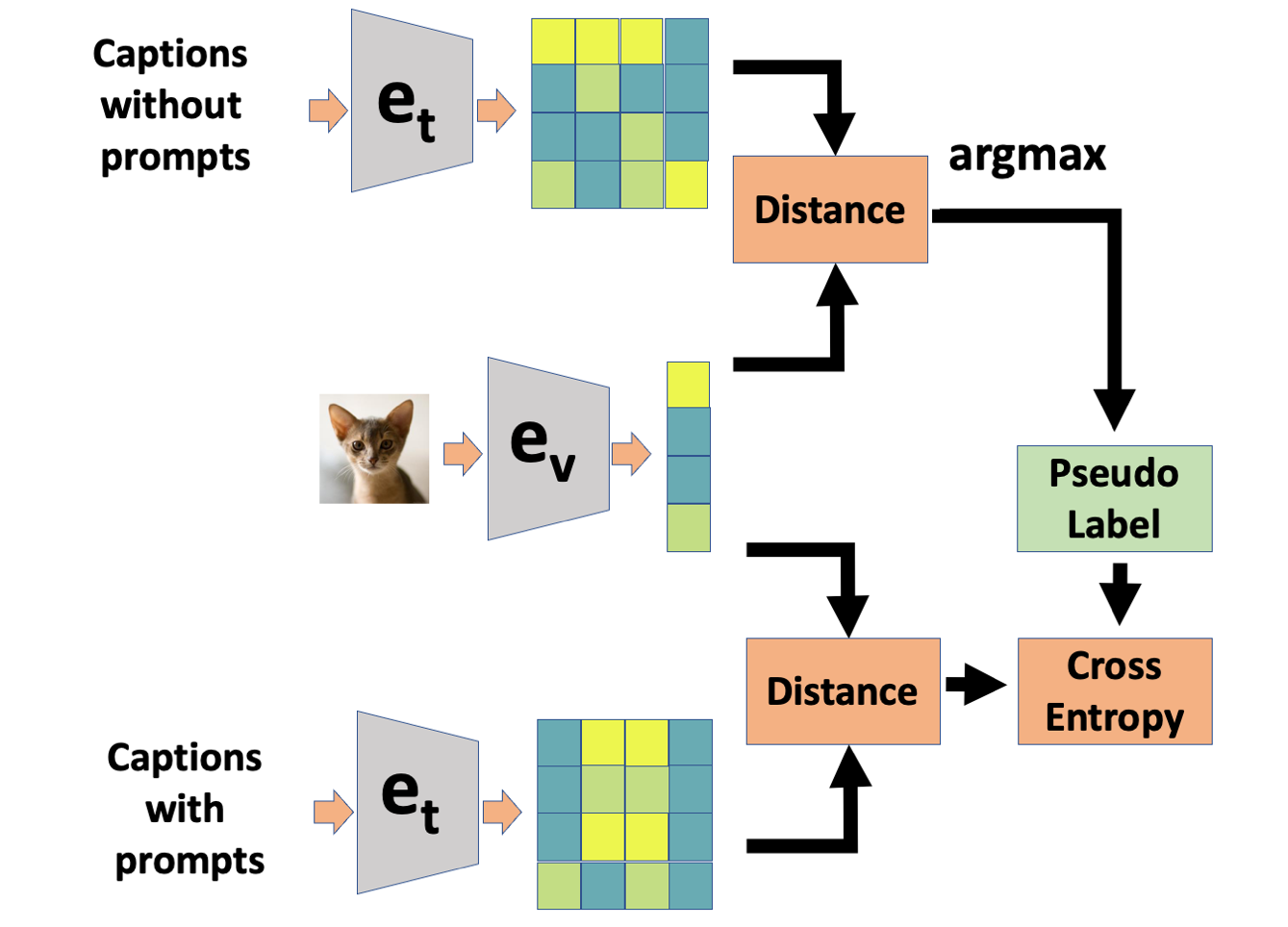
Figure 4: Overview of regularization. First, text prompts corresponding to some support classes are passed without prompts through the text encoder $e_{t}$. Distance between text feature and image features are used to determine the pseudo label among support classes. Then, text prompts of the same set of support classes are passed through the text encoder after appending prompts. Cross entropy loss is used to ensure that text feature of the pseudo labelled support class has the lowest distance with respect to the same image feature. This regularization ensures pre-existing relations that existed in the pretrained vocabulary (with respect to support classes) are maintained during prompt tuning.

Class-agnostic Regularization. Class-agnostic regularization is a more generic form of regularization that can be applied to any type of a classifier. This form of regularization uses a pre-defined static set of generic classes as support classes to maintain grounding with the pre-trained model. For example, in our experiments we considered [material, animal, food, dress, place, vehicle, plant, object] to be the support class list. We construct text features for support classes without prompts, and obtain a pseudo ground truth annotation by considering highest correlation to a given image feature as shown in Fig 4. Then, we generate text embeddings for the support set with soft prompts, and force the pseudo ground truth class to have the highest correlation with image features.

1. Let $\mathcal{Y}^{A}=[y^{A}_{1},y^{A}_{2},\dots,y^{A}_{k}]$ be the set of generic classes (support classes) identified.

2. For a given image $I$, consider $k$ sets of text prompts of the form $t_{l}=[t_{common},y^{A}_{l}]$ not including the soft-prompt token.

3. We search for the index $l^{*}=\arg\min_{l}d(e_{v}(I),e_{t}(t_{l}))$ of the pseudo-ground truth label $y^{A}_{l^{*}}$ that minimizes the distance between image and text features.

4. Then, a second set of text prompts are generated with the soft-prompt token of the form on $t_{l}^{v}=[t_{common},v_{j},y_{l}^{A}]$.

5. Finally, distance between image feature $e_{v}(I)$ and text-feature $e_{t}(t^{v}_{l})$ is calculated for each class. Considering these distance values to be class logits, cross entropy loss is calculated with respect to the pseudo-attribute label $y^{A}_{l^{*}}$.

In both forms of regularization, we record the response of the pre-trained model with respect to support classes and ensure, the same response is obtained when soft prompts are introduced. In order for these regularizations to be effective support class set should be different from the classifier classes.

5 Experiments

We evaluate the effectiveness of the proposed method on standard object classification datasets and object-attribute datasets. In all datasets, we identify two sets of super-classes and train two models for each super-class independently. In our evaluations we investigate how well a classifier composed with prompt algebra performs on these separate classification tasks. For Object Classification datasets we compare performance of vanilla prompt algebra with models trained with class-agnostic regularization. For object-attribute datasets, we consider both types of regularization.

5.1 Model Details.

We use CLIP ViT-L/14 model as our backbone architechture. In all our experiments we used a single prompt for prompt tuning. We selected the eigenspace by considering 0.9% of the spectral energy. In all experiments we gave equal weights to each prompt when performing prompt algebra. Each model was trained for 20 epochs with a dropout of 0.3 on prompt elements. We used an effective batch size of 512. The model was optimized with SGD with a learning rate of 0.01. For all experiments we considered three trials of experiments and report average performance (with standard deviation within brackets).

5.2 Performance on Attribute-Object Classification datasets

We use multi-view datasets to analyze performance of the proposed method as a union of task classifier and product of task classifier. Both MIT-states[9] and UTZappos[38] has object-attribute annotations for each data sample. We consider objects and attributes as two separate views of data for our analysis. The product space between these two views results in composite classes. For example, product of attribute young and object cat results in the composite class young cat.

MIT-states contains images of naturally occurring objects where each object is described by an adjective. It contains 115 attribute classes and 245 object classes. In total, there are images belonging to 1962 composite classes. UT-Zappos contains images of shoes paired with attributes that describe the shoe. The dataset consists of 12 object classes and 16 attribute types and 118 composite object-attribute classes. For both these datasets we used the splits used in [25] for bench-marking. In all datasets, only a selected few object-attribute combinations appear during training. These composite classes are named as seen-classes. Composite classes that appear only during testing are termed as unseen-classes. For object-attribute classification there is no notion of seen/unseen classes as all objects and attributes are observed during training.

For evaluation, we train classifiers for each modality for all datasets. During inference, we evaluate model performance on three criteria: test accuracy on the same modality, zero shot accuracy on cross modality, and zero shot performance on composite object-attribute task. We report best seen, best unseen and AUC metrics [25] following closed-set protocol. For each method, we report performance obtained from base classifiers as well as composite classifier obtained with prompt algebra.

In Table 1, we tabulate results obtained with UTZappos dataset. Interestingly, these results suggest that a object classifier trained on this dataset elevates attribute recognition performance over the CLIP baseline and vice versa. It should be noted attribute annotations were not used in any capacity when the object classifier is trained. This phenomena can be observed even on MIT-states datasets as evident in Table 2. This could be due to the fact that object and attribute recognition is inter-related. Therefore, when a classifier is trained to learn features that are important for attribute classification, it inadvertently learns features useful for object classification - there by improving zero-shot object recognition performance.

Without any regularization, prompt algebra has produced a classifier with average performance on both views for UTZappos. Regularization further improves performance of this classifier. In particular, performance of the composite classifier on attribute recognition is better than the base attribute classifier. A similar gain can be observed in composite-class classification tasks (for seen and unseen pair accuracy). This is one of the rare cases where combining classifiers of two views have resulted in a synergy.

On the other hand, performance gain of the composite classifier is not significant for MIT-states dataset. Regularization has improved attribute and object classification performance by 3.25% and 1.39% respectively. Seen and unseen object-attribute pair recognition has improved by approximately 2%. This is partly due to the fact there exist a stronger correlation between objects and attributes in this dataset. For an example, an object classifier has a zero shot attribute recognition accuracy of 22.22%; this is just 4.2% worse than a specialized attribute classifier.

		Attribute Accuracy	Object Accuracy	Seen Pair Accuracy	Unseen Pair Accuracy	AUC (Pair)
CLIP Zero Shot		12.01	48.76	15.74	49.23	5.00
Prompt Tuning	Obj. Classifier	27.22 (2.07)	53.20 (0.82)	16.78 (0.83)	51.54 (1.40)	6.20 (0.39)
	Att. Classifier	43.93 (0.51)	34.18 (2.77)	10.62 (0.06)	51.40 (0.92)	4.18 (0.02)
	Prompt Algebra	38.76 (3.04)	48.10 (0.81)	20.66 (0.76)	50.52 (1.16)	7.06 (0.67)
MV-Regularization	Obj. Classifier	13.77 (0.20)	48.26 (0.52)	22.29 (1.92)	50.77 (0.41)	7.73 (0.90)
	Att. Classifier	38.49 (0.61)	39.40 (1.96)	10.52 (0.45)	50.68 (0.34)	3.27 (0.10)
	Prompt Algebra	47.48 (0.81)	47.70 (0.69)	22.68 (1.96)	50.91 (0.54)	8.13 (0.98)
CA-Regularization	Obj. Classifier	28.25 (1.61)	51.90 (1.35)	12.15 (0.76)	48.81 (0.32)	4.21 (0.18)
	Att. Classifier	40.60 (0.05)	30.30 (3.40)	10.90 (0.48)	52.75 (1.08)	4.44 (0.17)
	Prompt Algebra	46.58 (0.49)	48.68 (0.58)	25.61 (2.14)	53.46 (1.64)	9.48 (1.45)

Table 1: Performance on UTZappos Dataset

		Attribute Accuracy	Object Accuracy	Seen Pair Accuracy	Unseen Pair Accuracy	AUC (Pair)
CLIP Zero Shot		15.78	40.85	30.50	46.08	11.00
Prompt Tuning	Obj. Classifier	22.22 (0.49)	52.40 (0.07)	32.54 (0.27)	48.16 (0.12)	12.59 (0.04)
	Att. Classifier	26.43 (0.49)	46.74 (0.57)	31.09 (0.30)	47.42 (0.73)	12.11 (0.16)
	Prompt Algebra	21.57 (0.95)	48.72 (0.76)	31.27 (0.68)	46.83 (0.30)	11.68 (0.39)
MV-Regularization	Obj. Classifier	23.02 (0.03)	51.81 (0.02)	31.91 (0.03)	46.34 (0.06)	12.04 (0.01)
	Att. Classifier	26.00 (1.15)	48.45 (0.02)	33.26 (1.04)	48.36 (0.57)	13.09 (0.37)
	Prompt Algebra	23.50 (0.50)	49.43 (0.81)	33.00 (0.56)	48.21 (0.24)	12.99 (0.08)
CA-Regularization	Obj. Classifier	22.85 (0.23)	52.29 (0.08)	32.56 (0.12)	48.36 (0.09)	12.77 (0.03)
	Att. Classifier	26.67 (0.67)	48.18 (0.16)	32.18 (0.59)	47.71 (0.09)	12.70 (0.14)
	Prompt Algebra	24.32 (0.83)	50.11 (0.59)	33.51 (0.80)	48.05 (0.21)	13.01 (0.43)

Table 2: Performance on MIT-states Dataset

5.3 Performance on Object Classification datasets.

We use CIFAR10[12] and CIFAR100[13] as benchmarks for object classification. In these datasets, we study how effective the proposed method is in creating a classifier that supports union of tasks. Specifically, we group all classes in these datasets into two super-classes: natural objects and artificial objects. CIFAR10 and CIFAR100 has 6(out of 10) and 31(out of 100) classes that qualify as natural objects. We train two classifiers independently: one on natural objects and the other on artificial objects. Results obtained for natural object classification, artificial object classification and overall classification performance is tabulated in Tables 3 and 4.

On CIFAR10 dataset, even the pretrained CLIP model exhibits very good zero shot performance. However object classifiers (for both natural and artificial image classes) improves on zero-shot performances of the in-domain data-split by about 2%. When a composite classifier is created with prompt algebra, it ends up producing marginally better overall classification performance (by 0.3%). Adding Regularization had further improved overall classification performance by a 0.3%. The table suggests that prompt algebra had produced a classifier that operates in-between a the two base classifiers. It’s performance is better than what base classifiers have achieved for cross-split testing.

CIFAR100 exhibits a similar trend to CIFAR10. Prompt algebra has improved best over-all classification performance by 2.6% in this dataset. Regularization has decreased performance by about 0.5% compared to the unregulated version. This could be due to the fact nominal classes used for regularization has higher correlation to CIFAR100 classes. In both datasets, performance of the composite classifier is within $1\%$ of the best base classifier.

		Artificial Objects Accuracy	Natural Object Accuracy	Overall Accuracy
CLIP Zero Shot		96.55	94.67	94.99
Prompt Tuning	Artificial Obj. Classifier	98.63 (0.07)	94.61 (0.47)	96.04 (0.28)
	Natural Obj. Classifier	93.37 (0.79)	96.57 (0.12)	95.09 (0.27)
	Prompt Algebra	97.51 (1.18)	95.77 (0.35)	96.29 (0.69)
CA-Regularization	Artificial Obj. Classifier	98.54 (0.08)	93.79 (0.31)	95.52 (0.16)
	Natural Obj. Classifier	96.71 (0.85)	96.77 (0.18)	96.54 (0.38)
	Prompt Algebra	98.25 (0.25)	95.87 (0.10)	96.64 (0.12)

Table 3: Results on CIFAR10 Dataset

		Artificial Objects Accuracy	Natural Object Accuracy	Overall Accuracy
CLIP Zero Shot		65.43	74.71	65.28
Prompt Tuning	Artificial Obj. Classifier	78.27 (0.34)	81.47 (0.20)	77.93 (0.46)
	Natural Obj. Classifier	73.67 (0.39)	88.02 (0.66)	78.93 (0.47)
	Prompt Algebra	76.99 (0.28)	86.83 (0.86)	78.93 (0.47)
CA-Regularization	Artificial Obj. Classifier	78.64 (0.70)	83.73 (1.42)	78.91 (0.78)
	Natural Obj. Classifier	74.67 (0.16)	88.30 (0.21)	77.53 (0.03)
	Prompt Algebra	76.89 (0.15)	86.52 (0.23)	78.77 (0.10)

Table 4: Results on CIFAR100 Dataset

	10 steps
	Average	Last
DER (w/o P) [36]	75.36 (0.36)	65.22
DER [36]	74.64 (0.28)	64.35
DyTox [6]	67.33 (0.02)	51.68
DyTox+ [6]	74.1 (0.10)	62.34
Continual CLIP [33]	75.17 (-)	66.72
Continual CLIP (our run)	77.48 (0.09)	65.28
Prompt Algebra	85.29 (0.05)	80.10
Prompt Algebra(CA)	84.37 (0.07)	76.87

Table 5: Continual learning results on CIFAR100 Dataset

5.4 Continual Learning Performance.

Class Incremental Learning (CIL) is different from our problem setting. Both settings set to solve classification problem in a union of tasks setting. However, information is shared between two tasks in CIL, whereas there is no information shared between models in our setting. Nevertheless, we tried to apply prompt algebra on a CIL task to test its applicability.

For this experiment we use CIFAR100-10 step protocol. In this protocol a model is initially trained on 10 classes. Then, the model encounters 10 new classes at a time - where it is expected to adapt new data while maintaining it’s expertise on older classes. Performance is evaluated by considering average performance across all splits and classification accuracy at the end of training (denoted as final).

We used prompt algebra to solve CIL task by training a new prompt for every split of 10 classes. We combined trained prompts (with equal weight) to obtain a composite classifier. In Table 5, we compare performance obtained with out method with recent state-of-the as reference. Here we show that prompt algebra out-performs continual CLIP[33] by more than 7% in average. It should be noted that regularization resulted in slightly worse performance than vanilla prompt algebra for this task.

5.5 Ablation Study

In this section, we analyze design choices made in the proposed method. For a ablation of spectral energy, number of prompts and weight of the regularization please refer the supplementary materials.

Impact of Regularization. In Table 6 we analyzed the impact of each component of regularization with a single trial of experiments on UTZappos dataset. Note that performance numbers of ablation study is different from results in the main section. According to Table 6, adding MV-regularization improved average recognition performance by over 3%. Training classifier with Eigen projection has resulted an improvement over 5%. When both forms of regularization are added average model performance increases by almost 6%. This study shows that each regularization step positively impacts model performance and that they can be used together when training a model to a good effect.

Impact of Prompt Weight Coefficients. In the main result section we consider equal weights when using prompt algebra on trained prompts. In this sub-section we explore the impact of using a different weight combination on UTZappos dataset. In Figure 5 we have plot object recognition performance of object classifier, attribute classifier and composite classifier for different combinations of weights. This figure suggests that performance curves are not always linear. For an example, prompt algebra for regularized model has a peak around 0.5 in the performance curve. This indicates that it’s possible to find synergies in composite models if weights are manually tuned.

Eigen Space Projection	MV- Regularization	Model	Attribute Accuracy	Object Accuracy	Average
✗	✗	Obj. Classifier	14.76	40.01	27.39
		Att. Classifier	43.21	37.75	40.48
		Prompt Algebra	42.79	40.56	41.68
✓	✗	Obj. Classifier	28.17	52.20	40.19
		Att. Classifier	41.73	31.26	36.50
		Prompt Algebra	45.92	48.76	47.34
✗	✓	Obj. Classifier	13.80	45.23	29.51
		Att. Classifier	39.12	35.66	37.39
		Prompt Algebra	45.92	44.03	44.97
✓	✓	Obj. Classifier	12.90	47.36	30.13
		Att. Classifier	40.73	35.18	37.95
		Prompt Algebra	48.11	47.15	47.63

Table 6: Ablation study on different components of regularization.

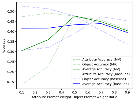
Figure 5: Impact of using different weights to combine object-attribute classifiers using prompt algebra on UTZappos dataset.

6 Conclusion

Our experimental results suggest that prompts trained with vanilla prompt tuning on a single view in a multi-view dataset (such as object-attribute datasets), elevates zero-shot performance of the second view. Once prompts are combined through algebraic operations, the composite classifier exhibits on par performance on both views as well as the composite view with respect to the base classifier. This observation continues to hold true even when classifiers with different class support are combined with prompt algebra (as in the case of CIFAR10/100 experiments). We observe that the proposed constrained prompt learning scheme further boosts performance of the composite classifier. In the future, we hope to extend this method to multiple prompts and explore an automated weight assignment mechanism for combining different prompts.

References

- [1] Jean-Baptiste Alayrac, Jeff Donahue, Pauline Luc, Antoine Miech, Iain Barr, Yana Hasson, Karel Lenc, Arthur Mensch, Katie Millican, Malcolm Reynolds, Roman Ring, Eliza Rutherford, Serkan Cabi, Tengda Han, Zhitao Gong, Sina Samangooei, Marianne Monteiro, Jacob Menick, Sebastian Borgeaud, Andrew Brock, Aida Nematzadeh, Sahand Sharifzadeh, Mikolaj Binkowski, Ricardo Barreira, Oriol Vinyals, Andrew Zisserman, and Karen Simonyan. Flamingo: a visual language model for few-shot learning, 2022.
- [2] Tom Brown, Benjamin Mann, Nick Ryder, Melanie Subbiah, Jared D Kaplan, Prafulla Dhariwal, Arvind Neelakantan, Pranav Shyam, Girish Sastry, Amanda Askell, Sandhini Agarwal, Ariel Herbert-Voss, Gretchen Krueger, Tom Henighan, Rewon Child, Aditya Ramesh, Daniel Ziegler, Jeffrey Wu, Clemens Winter, Chris Hesse, Mark Chen, Eric Sigler, Mateusz Litwin, Scott Gray, Benjamin Chess, Jack Clark, Christopher Berner, Sam McCandlish, Alec Radford, Ilya Sutskever, and Dario Amodei. Language models are few-shot learners. In H. Larochelle, M. Ranzato, R. Hadsell, M.F. Balcan, and H. Lin, editors, Advances in Neural Information Processing Systems, volume 33, pages 1877–1901. Curran Associates, Inc., 2020.
- [3] Aakanksha Chowdhery, Sharan Narang, Jacob Devlin, Maarten Bosma, Gaurav Mishra, Adam Roberts, Paul Barham, Hyung Won Chung, Charles Sutton, Sebastian Gehrmann, Parker Schuh, Kensen Shi, Sasha Tsvyashchenko, Joshua Maynez, Abhishek Rao, Parker Barnes, Yi Tay, Noam Shazeer, Vinodkumar Prabhakaran, Emily Reif, Nan Du, Ben Hutchinson, Reiner Pope, James Bradbury, Jacob Austin, Michael Isard, Guy Gur-Ari, Pengcheng Yin, Toju Duke, Anselm Levskaya, Sanjay Ghemawat, Sunipa Dev, Henryk Michalewski, Xavier Garcia, Vedant Misra, Kevin Robinson, Liam Fedus, Denny Zhou, Daphne Ippolito, David Luan, Hyeontaek Lim, Barret Zoph, Alexander Spiridonov, Ryan Sepassi, David Dohan, Shivani Agrawal, Mark Omernick, Andrew M. Dai, Thanumalayan Sankaranarayana Pillai, Marie Pellat, Aitor Lewkowycz, Erica Moreira, Rewon Child, Oleksandr Polozov, Katherine Lee, Zongwei Zhou, Xuezhi Wang, Brennan Saeta, Mark Diaz, Orhan Firat, Michele Catasta, Jason Wei, Kathy Meier-Hellstern, Douglas Eck, Jeff Dean, Slav Petrov, and Noah Fiedel. Palm: Scaling language modeling with pathways, 2022.
- [4] Jacob Devlin, Ming-Wei Chang, Kenton Lee, and Kristina Toutanova. BERT: Pre-training of deep bidirectional transformers for language understanding. In Proceedings of the 2019 Conference of the North American Chapter of the Association for Computational Linguistics: Human Language Technologies, Volume 1 (Long and Short Papers), pages 4171–4186, Minneapolis, Minnesota, June 2019. Association for Computational Linguistics.
- [5] Alexey Dosovitskiy, Lucas Beyer, Alexander Kolesnikov, Dirk Weissenborn, Xiaohua Zhai, Thomas Unterthiner, Mostafa Dehghani, Matthias Minderer, Georg Heigold, Sylvain Gelly, Jakob Uszkoreit, and Neil Houlsby. An image is worth 16x16 words: Transformers for image recognition at scale. In International Conference on Learning Representations, 2021.
- [6] Arthur Douillard, Alexandre Ramé, Guillaume Couairon, and Matthieu Cord. Dytox: Transformers for continual learning with dynamic token expansion. In Proceedings of the IEEE/CVF Conference on Computer Vision and Pattern Recognition (CVPR), pages 9285–9295, June 2022.
- [7] Gabriel Goh, Nick Cammarata, Chelsea Voss, Shan Carter, Michael Petrov, Ludwig Schubert, Alec Radford, , and Chris Olah. Multimodal neurons in artificial neural networks, 2021.
- [8] K. He, X. Zhang, S. Ren, and J. Sun. Deep residual learning for image recognition. In IEEE Conference on Computer Vision and Pattern Recognition, pages 770–778, June 2016.
- [9] Phillip Isola, Joseph J. Lim, and Edward H. Adelson. Discovering states and transformations in image collections. In CVPR, 2015.
- [10] Chao Jia, Yinfei Yang, Ye Xia, Yi-Ting Chen, Zarana Parekh, Hieu Pham, Quoc V. Le, Yunhsuan Sung, Zhen Li, and Tom Duerig. Scaling up visual and vision-language representation learning with noisy text supervision. 2021.
- [11] Menglin Jia, Luming Tang, Bor-Chun Chen, Claire Cardie, Serge Belongie, Bharath Hariharan, and Ser-Nam Lim. Visual prompt tuning, 2022.
- [12] Alex Krizhevsky, Vinod Nair, and Geoffrey Hinton. Cifar-10 (canadian institute for advanced research).
- [13] Alex Krizhevsky, Vinod Nair, and Geoffrey Hinton. Cifar-100 (canadian institute for advanced research).
- [14] Hunsang Lee, Hyesong Choi, Kwanghoon Sohn, and Dongbo Min. Knn local attention for image restoration. In Proceedings of the IEEE/CVF Conference on Computer Vision and Pattern Recognition (CVPR), pages 2139–2149, June 2022.
- [15] Brian Lester, Rami Al-Rfou, and Noah Constant. The power of scale for parameter-efficient prompt tuning. In Proceedings of the 2021 Conference on Empirical Methods in Natural Language Processing, pages 3045–3059, Online and Punta Cana, Dominican Republic, Nov. 2021. Association for Computational Linguistics.
- [16] Junnan Li, Ramprasaath R. Selvaraju, Akhilesh Deepak Gotmare, Shafiq Joty, Caiming Xiong, and Steven Hoi. Align before fuse: Vision and language representation learning with momentum distillation. In A. Beygelzimer, Y. Dauphin, P. Liang, and J. Wortman Vaughan, editors, Advances in Neural Information Processing Systems, 2021.
- [17] Xiang Lisa Li and Percy Liang. Prefix-tuning: Optimizing continuous prompts for generation. In Chengqing Zong, Fei Xia, Wenjie Li, and Roberto Navigli, editors, Proceedings of the 59th Annual Meeting of the Association for Computational Linguistics and the 11th International Joint Conference on Natural Language Processing, ACL/IJCNLP 2021, (Volume 1: Long Papers), Virtual Event, August 1-6, 2021, pages 4582–4597. Association for Computational Linguistics, 2021.
- [18] Pengfei Liu, Weizhe Yuan, Jinlan Fu, Zhengbao Jiang, Hiroaki Hayashi, and Graham Neubig. Pre-train, prompt, and predict: A systematic survey of prompting methods in natural language processing. ACM Comput. Surv., aug 2022. Just Accepted.
- [19] Xiao Liu, Kaixuan Ji, Yicheng Fu, Weng Tam, Zhengxiao Du, Zhilin Yang, and Jie Tang. P-tuning: Prompt tuning can be comparable to fine-tuning across scales and tasks. In Proceedings of the 60th Annual Meeting of the Association for Computational Linguistics (Volume 2: Short Papers), pages 61–68, Dublin, Ireland, May 2022. Association for Computational Linguistics.
- [20] Yinhan Liu, Myle Ott, Naman Goyal, Jingfei Du, Mandar Joshi, Danqi Chen, Omer Levy, Mike Lewis, Luke Zettlemoyer, and Veselin Stoyanov. Roberta: A robustly optimized BERT pretraining approach. CoRR, abs/1907.11692, 2019.
- [21] Jiasen Lu, Dhruv Batra, Devi Parikh, and Stefan Lee. Vilbert: Pretraining task-agnostic visiolinguistic representations for vision-and-language tasks. In Hanna M. Wallach, Hugo Larochelle, Alina Beygelzimer, Florence d’Alché Buc, Emily B. Fox, and Roman Garnett, editors, NeurIPS, pages 13–23, 2019.
- [22] Tomas Mikolov, Kai Chen, Greg S. Corrado, and Jeffrey Dean. Efficient estimation of word representations in vector space, 2013.
- [23] Ishan Misra, Abhinav Gupta, and Martial Hebert. From red wine to red tomato: Composition with context. In Proceedings of the IEEE Conference on Computer Vision and Pattern Recognition (CVPR), July 2017.
- [24] MF Naeem, Y Xian, F Tombari, and Zeynep Akata. Learning graph embeddings for compositional zero-shot learning. In 34th IEEE Conference on Computer Vision and Pattern Recognition. IEEE, 2021.
- [25] Nihal V. Nayak, Peilin Yu, and Stephen H. Bach. Learning to compose soft prompts for compositional zero-shot learning, 2022.
- [26] Senthil Purushwalkam, Maximilian Nickel, Abhinav Gupta, and Marc’Aurelio Ranzato. Task-driven modular networks for zero-shot compositional learning, 2019.
- [27] Alec Radford, Jong Wook Kim, Chris Hallacy, Aditya Ramesh, Gabriel Goh, Sandhini Agarwal, Girish Sastry, Amanda Askell, Pamela Mishkin, Jack Clark, Gretchen Krueger, and Ilya Sutskever. Learning transferable visual models from natural language supervision. In Marina Meila and Tong Zhang, editors, Proceedings of the 38th International Conference on Machine Learning, volume 139 of Proceedings of Machine Learning Research, pages 8748–8763. PMLR, 18–24 Jul 2021.
- [28] Alec Radford, Jeff Wu, Rewon Child, David Luan, Dario Amodei, and Ilya Sutskever. Language models are unsupervised multitask learners. 2019.
- [29] Sylvestre-Alvise Rebuffi, Alexander Kolesnikov, Georg Sperl, and Christoph H. Lampert. iCaRL: incremental classifier and representation learning. In CVPR, 2017.
- [30] Frank Ruis, Gertjan J. Burghouts, and Doina Bucur. Independent prototype propagation for zero-shot compositionality. In A. Beygelzimer, Y. Dauphin, P. Liang, and J. Wortman Vaughan, editors, Advances in Neural Information Processing Systems, 2021.
- [31] Weijie Su, Xizhou Zhu, Yue Cao, Bin Li, Lewei Lu, Furu Wei, and Jifeng Dai. VL-BERT: pre-training of generic visual-linguistic representations. In 8th International Conference on Learning Representations, ICLR 2020, Addis Ababa, Ethiopia, April 26-30, 2020. OpenReview.net, 2020.
- [32] Yoad Tewel, Yoav Shalev, Idan Schwartz, and Lior Wolf. Zero-shot image-to-text generation for visual-semantic arithmetic. arXiv preprint arXiv:2111.14447, 2021.
- [33] Vishal Thengane, Salman Khan, Munawar Hayat, and Fahad Khan. Clip model is an efficient continual learner. arXiv:2210.03114, 2022.
- [34] Gido M. van de Ven and Andreas Savas Tolias. Three scenarios for continual learning. ArXiv, abs/1904.07734, 2019.
- [35] Yabin Wang, Zhiwu Huang, and Xiaopeng Hong. S-prompts learning with pre-trained transformers: An occam’s razor for domain incremental learning. CoRR, abs/2207.12819, 2022.
- [36] Shipeng Yan, Jiangwei Xie, and Xuming He. Der: Dynamically expandable representation for class incremental learning. In CVPR, pages 3014–3023, 2021.
- [37] Mohit Bansal Yi-Lin Sung, Jaemin Cho. Vl-adapter: Parameter-efficient transfer learning for vision-and-language tasks. In CVPR, 2022.
- [38] Aron Yu and Kristen Grauman. Fine-grained visual comparisons with local learning. In 2014 IEEE Conference on Computer Vision and Pattern Recognition, pages 192–199, 2014.
- [39] Sergey Zagoruyko and Nikos Komodakis. Wide residual networks. In Bmvc, 2016.