Low-Light Image Enhancement with Wavelet-based Diffusion Models

Abstract.

Diffusion models have achieved promising results in image restoration tasks, yet suffer from time-consuming, excessive computational resource consumption, and unstable restoration. To address these issues, we propose a robust and efficient Diffusion-based Low-Light image enhancement approach, dubbed DiffLL. Specifically, we present a wavelet-based conditional diffusion model (WCDM) that leverages the generative power of diffusion models to produce results with satisfactory perceptual fidelity. Additionally, it also takes advantage of the strengths of wavelet transformation to greatly accelerate inference and reduce computational resource usage without sacrificing information. To avoid chaotic content and diversity, we perform both forward diffusion and denoising in the training phase of WCDM, enabling the model to achieve stable denoising and reduce randomness during inference. Moreover, we further design a high-frequency restoration module (HFRM) that utilizes the vertical and horizontal details of the image to complement the diagonal information for better fine-grained restoration. Extensive experiments on publicly available real-world benchmarks demonstrate that our method outperforms the existing state-of-the-art methods both quantitatively and visually, and it achieves remarkable improvements in efficiency compared to previous diffusion-based methods. In addition, we empirically show that the application for low-light face detection also reveals the latent practical values of our method. Code is available at https://github.com/JianghaiSCU/Diffusion-Low-Light.

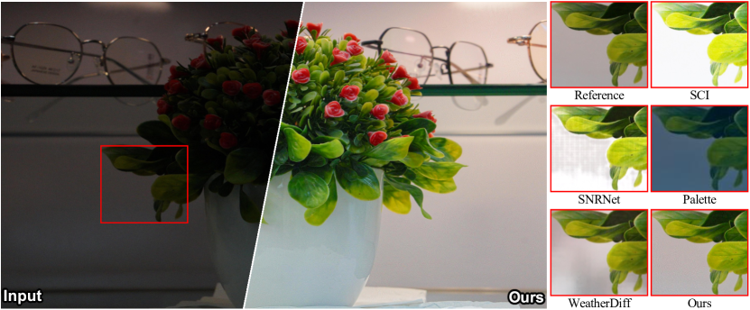
Figure 1. Visual comparisons of recent state-of-the-art unsupervised and supervised low-light image enhancement methods SCI (Ma et al., 2022) and SNRNet (Xu et al., 2022), two diffusion-based image restoration methods Palette (Saharia et al., 2022) and WeatherDiff (Özdenizci and Legenstein, 2023), and our method on an image with 2K resolution selected from the UHD-LL (Li et al., 2023) test set. Previous methods appear incorrect exposure, color distortion, or artifacts to degrade visual quality, while our method properly improves global contrast and presents a vivid color without introducing chaotic content.

1. Introduction

Images captured in weakly illuminated conditions suffer from unfavorable visual quality, which seriously impairs the performance of downstream vision tasks and practical intelligent systems, such as image classification (Loh and Chan, 2019), object detection (Liang et al., 2021), automatic driving (Li et al., 2021c), and visual navigation (Hai et al., 2021), etc. Numerous advances have been made in improving contrast and restoring details to transform low-light images into high-quality ones. Traditional approaches typically rely on optimization-based rules, with the effectiveness of these methods being highly dependent on the accuracy of hand-crafted priors. However, low-light image enhancement (LLIE) is inherently an ill-posed problem, as it presents difficulties in adapting such priors for various illumination conditions.

With the rise of deep learning, such problems have been partially solved, learning-based methods directly learn mappings between degraded images and corresponding high-quality sharp versions, thus being more robust than traditional methods. Learning-based methods can be divided into two categories: supervised and unsupervised. The former leverage large-scale datasets and powerful neural network architectures for restoration that aim to optimize distortion metrics such as PSNR and SSIM (Wang et al., 2004), while lacking visual fidelity for human perception. Unsupervised methods have better generalization ability for unseen scenes, benefiting from their label-free characteristics. Nevertheless, they are typically unable to control the degree of enhancement and may produce visually unappealing results in some cases, such as over-enhanced or noise amplification, as with supervised ones. As shown in Fig. 1, both unsupervised SCI (Ma et al., 2022) and supervised SNRNet (Xu et al., 2022) appear incorrectly overexposed in the background region.

Therefore, following perceptual-driven approaches (Johnson et al., 2016; Li et al., 2021b), deep generative models such as generative adversarial networks (GANs) (Jiang et al., 2021; Yang et al., 2022) and variational autoencoders (VAEs) (Zheng et al., 2022) have emerged as promising approaches for LLIE. These methods aim to capture multi-modal distributions of inputs to generate output images with better perceptual fidelity. Recently, diffusion models (DMs) (Sohl-Dickstein et al., 2015; Song et al., 2021b; Song and Ermon, 2019) have garnered attention due to their impressive performance in image synthesis (Ho et al., 2020; Song et al., 2021a) and restoration tasks (Luo et al., 2023b; Li et al., 2022). DMs rely on a hierarchical architecture of denoising autoencoders that enable them to iteratively reverse a diffusion process and achieve high-quality mapping from randomly sampled Gaussian noise to target images or latent distributions (Rombach et al., 2022), without suffering instability and mode-collapse present in previous generative models. Although standard DMs are capable enough, there exist several challenges for some image restoration tasks, especially for LLIE. As shown in Fig. 1, the diffusion-based methods Palette (Saharia et al., 2022) and WeatherDiff (Özdenizci and Legenstein, 2023) generate images with color distortion or artifacts, since the reverse process starts from a random sampled Gaussian noise, resulting in the final result may have unexpected chaotic content due to the diversity of the sampling process, despite conditional inputs can be used to constrain the output distribution. Moreover, DMs usually require extensive computational resources and long inference times to achieve effective iterative denoising, as shown in Fig. 2 (a), the diffusion-based methods take more than 10 seconds to restore an image with the size of 600$\times$400.

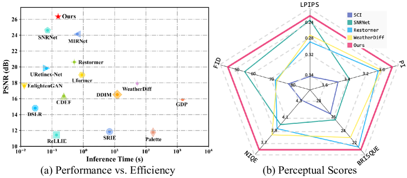
Figure 2. Quantitative comparisons with state-of-the-art methods. (a) presents the performance, i.e., PSNR, and inference time of comparison methods on the LOLv1 (Wei et al., 2018) test set, where the image size is 600$\times$400. (b) presents numerical scores for five perceptual metrics including LPIPS (Zhang et al., 2018), FID (Heusel et al., 2017), NIQE (Mittal et al., 2012b), BRISQUE (Mittal et al., 2012a), and PI (Blau et al., 2018) (the lower the scores the better the visual quality) on the LOLv1 test set and five real-world benchmarks including DICM (Lee et al., 2013), MEF (Ma et al., 2015), LIME (Guo et al., 2016), NPE (Wang et al., 2013), and VV. It can be easily observed that our method is remarkably superior to others, achieving state-of-the-art performance while being computational efficiency.

In this work, we propose a diffusion-based framework, named DiffLL, for robust and efficient low-light image enhancement. Specifically, we first convert the low-light image into the wavelet domain using $K$ times 2D discrete wavelet transformations (2D-DWT), which noticeably reduces the spatial dimension while avoiding information loss, resulting in an average coefficient that represents the global information of the input image and $K$ sets of high-frequency coefficients that represent sparse vertical, horizontal, and diagonal details of the image. Accordingly, we propose a wavelet-based conditional diffusion model (WCDM) that performs diffusion operations on the average coefficient instead of the original image space or latent space for the reduction of computational resource consumption and inference time. As depicted in Fig. 2 (a), our method achieves a speed that is over 70$\times$ faster than the previous diffusion-based method DDIM (Song et al., 2021a). In addition, during the training phase of the WCDM, we perform both the forward diffusion and the denoising processes. This enables us to fully leverage the generative capacity of the diffusion mode while teaching the model to conduct stable sampling during inference, preventing content diversity even with randomly sampled noise. As shown in Fig. 1, our method properly improves global contrast and prevents excessive correction on the well-exposed region, without any artifacts or chaotic content appearance. Besides, perceptual scores shown in Fig. 2 (b) also indicate that our method generates images with better visual quality. Furthermore, the local details contained in the high-frequency coefficients are reconstructed through our well-designed high-frequency restoration modules (HFRM), where the vertical and horizontal information is utilized to complement the diagonal details for better fine-grained details restoration which contributes to the overall quality. Extensive experiments on publicly available datasets show that our method outperforms the existing state-of-the-art (SOTA) methods in terms of both distortion and perceptual metrics, and offers notable improvements in efficiency compared to previous diffusion-based methods. The application for low-light face detection also reveals the potential practical values of our method. Our contributions can be summarized as follows:

• We propose a wavelet-based conditional diffusion model (WCDM) that leverages the generative ability of diffusion models and the strengths of wavelet transformation for robust and efficient low-light image enhancement.

• We propose a new training strategy that enables WCDM to achieve content consistency during inference by performing both the forward diffusion and the denoising processes in the training phase.

• We further design a high-frequency restoration module (HFRM) that utilizes both vertical and horizontal information to complement the diagonal details for local details reconstruction.

• Extensive experimental results on public real-world benchmarks show that our proposed method achieves state-of-the-art performance on both distortion metrics and perceptual quality while offering noticeable speed up compared to previous diffusion-based methods.

2. Related Work

2.1. Low-light Image Enhancement

To transform low-light images into visually satisfactory ones, numerous efforts have made considerable advances in improving contrast and restoring details. Traditional methods mainly adopt histogram equalization (HE) (Bovik, 2010) and Retinex theory (Land, 1977) to achieve image enhancement. HE-based methods (Singh et al., 2015; Park et al., 2022; Ooi and Isa, 2010) take effect by changing the histogram of the image to improve the contrast. Retinex-based methods (Lin and Shi, 2014; Fu et al., 2016; Jobson et al., 1997) decompose the image into an illumination map and a reflectance map, by changing the dynamic range of pixels in the illumination map and suppressing the noise in the reflectance map to improve the visual quality of the image. For example, LIME (Guo et al., 2016) utilized a weighted vibration model based on a prior hypothesis to adjust the estimated illumination, followed by BM3D (Dabov et al., 2007) as a post-processing step for noise removal.

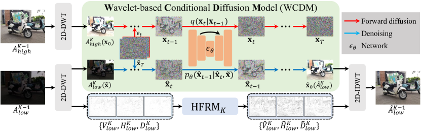
Figure 3. The overall pipeline of our proposed DiffLL. We first convert the low-light image into the wavelet domain using 2D discrete wavelet transformation (2D-DWT) in $K$ times, resulting in an average coefficient $A_{low}^{K}$ and $K$ sets of high-frequency coefficients $\{V_{low}^{k},H_{low}^{k},D_{low}^{k}\}$, where $k\in[1,K]$. The proposed wavelet-based conditional model (WCDM) performs diffusion operations on the average coefficient to achieve robust and efficient restoration, in which the training and inference strategies are detailed in ALGORITHM 1 and ALGORITHM 2, respectively. The forward diffusion process is only performed in the training phase and the denoising process is performed in both training and inference phases. Finally, the result at scale $k-1$ is obtained by converting the restored average coefficient and the high-frequency coefficients at scale $k$ using the 2D inverse discrete wavelet transformation (2D-IDWT).

Following the development of learning-based image restoration methods (Mao et al., 2016; Dong et al., 2015; Sun et al., 2015), LLNet (Lore et al., 2017) first proposed a deep encoder-decoder network for contrast enhancement and introduced a dataset synthesis pipeline. RetinexNet (Wei et al., 2018) introduced the first paired dataset captured in real-world scenes and combined Retinex theory with a CNN network to estimate and adjust the illumination map. EnlightenGAN (Jiang et al., 2021) adopted unpaired images for training for the first time by using the generative adverse network as the main framework. Zero-DCE (Guo et al., 2020) proposed to transform LLIE into a curve estimation problem and designed a zero-reference learning strategy for training. RUAS (Liu et al., 2021) proposed a Retinex-inspired architecture search framework to discover low-light prior architectures from a compact search space. SNRNet (Xu et al., 2022) utilized signal-to-noise-ratio-aware transformers and CNN models with spatial-varying operations for restoration. A more comprehensive survey can be found in (Li et al., 2021a).

2.2. Diffusion-based Image Restoration

Diffusion-based generative models have yielded encouraging results with improvements employed in denoising diffusion probability models (Ho et al., 2020), which become more impactful in image restoration tasks such as super-resolution (Luo et al., 2023a; Shang et al., 2023), inpainting (Lugmayr et al., 2022), and deblurring (Ren et al., 2022). DDRM (Kawar et al., 2022) used a pre-trained diffusion model to solve any linear inverse problem, which presented superior results over recent unsupervised methods on several image restoration tasks. ShadowDiffusion (Guo et al., 2023) designed an unrolling diffusion model that achieves robust shadow removal by progressively refining the results with degradation and generative priors. DR2 (Wang et al., 2023) first used a pre-trained diffusion model for coarse degradation removal, followed by an enhancement module for finer blind face restoration. WeatherDiff (Özdenizci and Legenstein, 2023) proposed a patch-based diffusion model to restore images captured in adverse weather conditions, which employed a guided denoising process across the overlapping patches in the inference process.

Although diffusion-based methods can obtain restored images with better visual quality than GAN-based and VAE-based generative approaches (Yang et al., 2021a; Peng et al., 2021), they often suffer from high computational resource consumption and inference time due to multiple forward and backward passes through the entire network. In this paper, we propose to combine diffusion models with wavelet transformation to noticeably reduce the spatial dimension of inputs in the diffusion process, achieving more efficient and robust low-light image enhancement.

3. Method

The overall pipeline of our proposed DiffLL is illustrated in Fig.  3. Our approach leverages the generative ability of diffusion models and the strengths of wavelet transformation to achieve visually satisfactory image restoration and improve the efficiency of diffusion models. The wavelet transformation can halve the spatial dimensions after each transformation without sacrificing information, while other transformation techniques, such as Fast Fourier Transformation (FFT) and Discrete Cosine Transform (DCT), are unable to achieve this level of reduction and may result in information loss. Therefore, we conduct diffusion operations on the wavelet domain instead of on the image space. In this section, we begin by presenting the preliminaries of 2D discrete wavelet transformation (2D-DWT) and conventional diffusion models. Then, we introduce the wavelet-based conditional diffusion model (WCDM), which forms the core of our approach. Finally, we present the high-frequency restoration module (HFRM), a well-designed component that contributes to local details reconstruction and improvement in overall quality.

3.1. Discrete Wavelet Transformation

Given a low-light image $I_{low}\in\mathbb{R}^{H\times W\times c}$, we use 2D discrete wavelet transformation (2D-DWT) with Haar wavelets (Haar, 1911) to transform the input into four sub-bands, i.e.,

(1) $$\{A_{low}^{1},V_{low}^{1},H_{low}^{1},D_{low}^{1}\}=\operatorname{2D-DWT}(I_{low}),$$

where $A_{low}^{1},V_{low}^{1},H_{low}^{1},D_{low}^{1}\in\mathbb{R}^{\frac{H}{2}\times\frac{W}{2}\times c}$ represent the average of the input image and high-frequency information in the vertical, horizontal, and diagonal directions, respectively. In particular, the average coefficient contains the global information of the original image, which can be treated as the downsampled version of the image, and the other three coefficients contain sparse local details. As shown in Fig. 4, the images reconstructed by exchanging high-frequency coefficients still have approximately the same content as the original images, whereas the image reconstructed by replacing the average coefficient changes the global information, resulting in the largest error with the original images. Therefore, the primary focus on restoring the low-light image in the wavelet domain is to obtain the average coefficient that has natural illumination consistent with its normal-light counterpart. For this purpose, we utilize the generative capability of diffusion models to restore the average coefficient, and the remaining three high-frequency coefficients are reconstructed through the proposed HFRM to facilitate local details restoration.

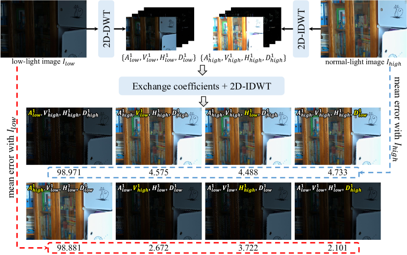
Figure 4. Illustration of exchanging wavelet coefficients between the low-light and normal-light images. Replacing the average coefficient in reconstructed images alters global illumination while exchanging high-frequency coefficients approximately retains the same content as the original images. The quantitative results in mean error also demonstrate that the average coefficient contains richer information than the high-frequency coefficients.

Although the spatial dimension of the wavelet component processed by the diffusion model after one wavelet transformation is four times smaller than the original image, we further perform $K-1$ times wavelet transformations on the average coefficient, i.e.,

(2) $$\{A_{low}^{k},V_{low}^{k},H_{low}^{k},D_{low}^{k}\}=\operatorname{2D-DWT}(A_{low}^{k-1}),$$

where $A_{low}^{k},V_{low}^{k},H_{low}^{k},D_{low}^{k}\in\mathbb{R}^{\frac{H}{2^{k}}\times\frac{W}{2^{k}}\times c}$, $k\in[1,K]$, and the original input image could be denoted as $A_{low}^{0}$. Subsequently, we do diffusion operations on the $A_{low}^{K}$ to further improve the efficiency, and the high-frequency coefficients $\{V_{low}^{k},H_{low}^{k},D_{low}^{k}\}$ are also reconstructed by the HFRM_k. In this way, our approach achieves significant decreases in inference time and computational resource consumption of the diffusion model due to $4^{K}$ times reduction in the spatial dimension.

3.2. Conventional Conditional Diffusion Models

Diffusion models (Song et al., 2021a; Ho et al., 2020) aim to learn a Markov Chain to gradually transform the distribution of Gaussian noise into the training data, which is generally divided into two phases: the forward diffusion and the denoising. The forward diffusion process first uses a fixed variance schedule $\{\beta_{1},\beta_{2},\cdots,\beta_{T}\}$ to progressively transform the input $\mathbf{x}_{0}$ into corrupted noise data $\mathbf{x}_{T}\sim\mathcal{N}(\mathbf{0},\mathbf{I})$ through $T$ steps, which can be formulated as:

(3) $$q(\mathbf{x}_{1:T}\mid\mathbf{x}_{0})=\prod_{t=1}^{T}q(\mathbf{x}_{t}\mid\mathbf{x}_{t-1}),$$

(4) $$q(\mathbf{x}_{t}\mid\mathbf{x}_{t-1})=\mathcal{N}(\mathbf{x}_{t};\sqrt{1-\beta_{t}}\mathbf{x}_{t-1},\beta_{t}\mathbf{I}),$$

where $\mathbf{x}_{t}$ and $\beta_{t}$ are the corrupted noise data and the pre-defined variance at time-step $t$, respectively, and $\mathcal{N}$ represents the Gaussian distribution.

The inverse process learns the Gaussian denoising transitions starting from the standard normal prior $p(\mathbf{\hat{x}}_{T})=\mathcal{N}(\mathbf{\hat{x}}_{T};\mathbf{0},\mathbf{I})$, and gradually denoise a randomly sampled Gaussian noise $\mathbf{\hat{x}}_{T}\sim\mathcal{N}(\mathbf{0},\mathbf{I})$ into a sharp result $\mathbf{\hat{x}}_{0}$, i.e.,

(5) $$p_{\theta}(\mathbf{\hat{x}}_{0:T})=p(\mathbf{\hat{x}}_{T})\prod_{t=1}^{T}p_{\theta}(\mathbf{\hat{x}}_{t-1}\mid\mathbf{\hat{x}}_{t}).$$

By applying the editing and data synthesis capabilities of conditional diffusion models (Chung et al., 2022), we aim to learn conditional denoising process $p_{\theta}(\mathbf{\hat{x}}_{0:T}\mid\tilde{\mathbf{x}})$ without changing the forward diffusion for $\mathbf{x}$, which results in high fidelity of the sampled result to the distribution conditioned on the conditional input $\tilde{\mathbf{x}}$. The Eq.5 is converted to:

(6) $$p_{\theta}(\mathbf{\hat{x}}_{0:T}\mid\tilde{\mathbf{x}})=p(\mathbf{\hat{x}}_{T})\prod_{t=1}^{T}p_{\theta}(\mathbf{\hat{x}}_{t-1}\mid\mathbf{\hat{x}}_{t},\tilde{\mathbf{x}}),$$

(7) $$p_{\theta}(\mathbf{\hat{x}}_{t-1}\mid\mathbf{\hat{x}}_{t})=\mathcal{N}(\mathbf{\hat{x}}_{t-1};\boldsymbol{\mu}_{\theta}(\mathbf{\hat{x}}_{t},t),\sigma_{t}^{2}\mathbf{I}).$$

The training objective for diffusion models is to optimize a network $\boldsymbol{\mu}_{\theta}(\mathbf{x}_{t},\tilde{\mathbf{x}},t)=\frac{1}{\sqrt{\alpha_{t}}}(\mathbf{x}_{t}-\frac{\beta_{t}}{\sqrt{1-\bar{\alpha}_{t}}}\boldsymbol{\epsilon}_{\theta}(\mathbf{x}_{t},\tilde{\mathbf{x}},t))$ that predicts $\tilde{\boldsymbol{\mu}}_{t}$, where the model can predict the noise vector $\boldsymbol{\epsilon}_{\theta}(\mathbf{x}_{t},\tilde{\mathbf{x}},t)$ by optimizing the network parameters $\theta$ of $\boldsymbol{\epsilon}_{\theta}$ like (Ho et al., 2020). The objective function is formulated as:

(8) $$\mathcal{L}_{diff}=E_{\mathbf{x}_{0},t,\epsilon_{t}\sim\mathcal{N}(\mathbf{0},\mathbf{I})}[\|\epsilon_{t}-\epsilon_{\theta}(\mathbf{x}_{t},\tilde{\mathbf{x}},t)\|^{2}].$$

3.3. Wavelet-based Conditional Diffusion Models

However, for some image restoration tasks, there are two challenges with the above conventional diffusion and reverse processes: 1) The forward diffusion with large time step $T$, typically set to $T=1000$, and small variance $\beta_{t}$ permits the assumption that the denoising process becomes close to Gaussian, which results in costly inference time and computational resources consumption. 2) Since the reverse process starts from a randomly sampled Gaussian noise, the diversity of the sampling process may lead to content inconsistency in the restored results, despite the conditioned input enforcing constraints on the distribution of the sampling results.

input : Average coefficients of low/normal-light image pairs $A_{low}^{K}$ and $A_{high}^{K}$, denoted as $\tilde{\mathbf{x}}$ and $\mathbf{x}_{0}$, respectively, the time step $T$, and the number of implicit sampling step $S$.

while Not converged do

      

      # Forward diffusion process

      $t\sim\operatorname{Uniform}\{1,\cdots,T\}$

      $\epsilon_{t}\sim\mathcal{N}(\mathbf{0},\mathbf{I})$

      Perform a single gradient descent step for $\nabla_{\theta}\|\boldsymbol{\epsilon}_{t}-\boldsymbol{\epsilon}_{\theta}(\sqrt{\bar{\alpha}_{t}}\mathbf{x}_{0}+\sqrt{1-\bar{\alpha}_{t}}\boldsymbol{\epsilon}_{t},\tilde{\mathbf{x}},t)\|^{2}$

      # Denoising process

      $\mathbf{\hat{x}}_{T}\sim\mathcal{N}(\mathbf{0},\mathbf{I})$

      for $i=S:1$ do

             $t=(i-1)\cdot T/S+1$

            $t_{\operatorname{next}}=(i-2)\cdot T/S+1$ if $i>1$, else $0$

            $\mathbf{\hat{x}}_{t}\leftarrow\sqrt{\bar{\alpha}_{t_{\operatorname{next}}}}(\frac{\mathbf{\hat{x}}_{t}-\sqrt{1-\bar{\alpha}_{t}}\cdot\epsilon_{\theta}(\mathbf{\hat{x}}_{t},\tilde{\mathbf{x}},t)}{\sqrt{\bar{\alpha}_{t}}})+\sqrt{1-\bar{\alpha}_{t_{\operatorname{next}}}}\cdot\epsilon_{\theta}(\mathbf{\hat{x}}_{t},\tilde{\mathbf{x}},t)$

       end for

      

      Perform a single gradient descent step for $\nabla_{\theta}\|\mathbf{\hat{x}}_{0}-\mathbf{x}_{0}\|^{2}$

end while

output : $\theta$, $\mathbf{\hat{x}}_{0}$ ($\hat{A}_{low}^{K}$)

ALGORITHM 1 Wavelet-based conditional diffusion model training

input : Average coefficients of low-light image $A_{low}^{k}$, denoted as $\tilde{\mathbf{x}}$, the time step $T$, and the number of implicit sampling step $S$.

# Denoising process

$\mathbf{\hat{x}}_{T}\sim\mathcal{N}(\mathbf{0},\mathbf{I})$

for $i=S:1$ do

       $t=(i-1)\cdot T/S+1$

      $t_{\operatorname{next}}=(i-2)\cdot T/S+1$ if $i>1$, else $0$

      $\mathbf{\hat{x}}_{t}\leftarrow\sqrt{\bar{\alpha}_{t_{\operatorname{next}}}}(\frac{\mathbf{\hat{x}}_{t}-\sqrt{1-\bar{\alpha}_{t}}\cdot\epsilon_{\theta}(\mathbf{\hat{x}}_{t},\tilde{\mathbf{x}},t)}{\sqrt{\bar{\alpha}_{t}}})+\sqrt{1-\bar{\alpha}_{t_{\operatorname{next}}}}\cdot\epsilon_{\theta}(\mathbf{\hat{x}}_{t},\tilde{\mathbf{x}},t)$

end for

output : $\mathbf{\hat{x}}_{0}$ ($\hat{A}_{low}^{k}$)

ALGORITHM 2 Wavelet-based conditional diffusion model inference

To address these problems, we propose a wavelet-based conditional diffusion model (WCDM) that converts the input low-light image $I_{low}$ into the wavelet domain and performs the diffusion process on the average coefficient, which considerably reduces the spatial dimension for efficient restoration. In addition, we perform both the forward diffusion and the denoising processes in the training phase, which aids the model in achieving stable sampling during inference and avoiding content diversity. The training approach of our wavelet-based conditional diffusion model is summarized in Algorithm 1. Specifically, we first perform the forward diffusion to optimize a noise estimator network via Eq.8, then adopt the sampled noise $\mathbf{\hat{x}}_{T}$ with conditioned input $\tilde{\mathbf{x}}$, i.e., the average coefficient $A_{low}^{K}$, for the denoising process, resulting in the restored coefficient $\hat{A}_{low}^{K}$. The content consistency is realized by minimizing the L2 distance between the restored coefficient and the reference coefficient $A_{high}^{K}$ which is only available during the training phase. Accordingly, the objective function Eq.8 used to optimize the diffusion model is rewritten as:

(9) $$\mathcal{L}_{diff}=E_{\mathbf{x}_{0},t,\epsilon_{t}\sim\mathcal{N}(\mathbf{0},\mathbf{I})}[\|\epsilon_{t}-\epsilon_{\theta}(\mathbf{x}_{t},\tilde{\mathbf{x}},t)\|^{2}]+\|\hat{A}_{low}^{K}-A_{high}^{K}\|^{2}.$$

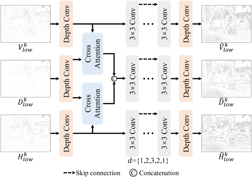
Figure 5. The detailed architecture of our proposed high-frequency restoration module. Depth Conv denotes the depth-wise separable convolution.

Discussion. There exist some diffusion models, such as Latent Diffusion (Rombach et al., 2022), that adopt VAE to transform the original image into the feature level and perform diffusion operations in the latent space, which can also achieve spatial dimension reduction as our method. However, encoding the original image through the VAE encoder inevitably causes information loss, whereas the wavelet transformation offers the advantage of preserving all information without any sacrifice. In addition, utilizing VAE would introduce an increase in model parameters, whereas the wavelet transformation, being a linear operation, does not incur additional resource consumption. On the other hand, the data typically used for training VAE are captured under normal-light conditions, it should be retrained on the low-light dataset to prevent domain shifts and maintain effective generation capability.

3.4. High-Frequency Restoration Module

For the $k$-th level wavelet sub-bands of the low-light image, the high-frequency coefficients $V_{low}^{k}$, $H_{low}^{k}$, and $D_{low}^{k}$ hold sparse representations of vertical, horizontal, and diagonal details of the image. To restore the low-light image to contain as rich information as the normal-light image, we propose a high-frequency restoration module (HFRM) to reconstruct these coefficients. As shown in Fig. 5, we first use three depth-wise separable convolutions (Chollet, 2017) for the sake of efficiency to extract the features of input coefficients, then two cross-attention layers (Hou et al., 2019) are employed to leverage the information in $V$ and $H$ to complement the details in $D$. Subsequently, inspired by (Hai et al., 2022), we design a progressive dilation Resblock utilizing dilation convolutions for local restoration, where the first and last convolutions are utilized to extract local information, and the middle dilation convolutions are used to improve the receptive field to make better use of long-range information. By gradually increasing and decreasing the dilation rate $d$, the gridding effect can be avoided. Finally, three depth-wise separable convolutions are used to reduce channels to obtain the reconstructed $\hat{V}_{low}^{k}$, $\hat{H}_{low}^{k}$, and $\hat{D}_{low}^{k}$. The restored average coefficient and the high-frequency coefficients at scale $k$ are correspondingly converted into the output at scale $k-1$ by employing the 2D inverse discrete wavelet transformation (2D-IDWT), i.e.,

(10) $$\hat{A}_{low}^{k-1}=\operatorname{2D-IDWT}(\{\hat{A}_{low}^{k},\hat{V}_{low}^{k},\hat{H}_{low}^{k},\hat{D}_{low}^{k}\}),$$

where the $\hat{A}_{low}^{0}$ denotes the final restored image $\hat{I}_{low}$.

Table 1. Quantitative evaluation of different methods on LOL-v1 (Wei et al., 2018), LOLv2-real (Yang et al., 2021b), and LSRW (Hai et al., 2023) test sets. The best results are highlighted in bold and the second best results are underlined. $\ast$ denotes the methods are retrained on the LOLv1 training set.

Methods	Reference	LOLv1				LOLv2-real				LSRW
		PSNR $\uparrow$	SSIM $\uparrow$	LPIPS $\downarrow$	FID $\downarrow$	PSNR $\uparrow$	SSIM $\uparrow$	LPIPS $\downarrow$	FID $\downarrow$	PSNR $\uparrow$	SSIM $\uparrow$	LPIPS $\downarrow$	FID $\downarrow$
NPE	TIP’ 13	16.970	0.484	0.400	104.057	17.333	0.464	0.396	100.025	16.188	0.384	0.440	90.132
SRIE	CVPR’ 16	11.855	0.495	0.353	88.728	14.451	0.524	0.332	78.834	13.357	0.415	0.399	69.082
LIME	TIP’ 16	17.546	0.531	0.387	117.892	17.483	0.505	0.428	118.171	17.342	0.520	0.471	75.595
RetinexNet	BMVC’ 18	16.774	0.462	0.417	126.266	17.715	0.652	0.436	133.905	15.609	0.414	0.454	108.350
DSLR	TMM’ 20	14.816	0.572	0.375	104.428	17.000	0.596	0.408	114.306	15.259	0.441	0.464	84.930
DRBN	CVPR’ 20	16.677	0.730	0.345	98.732	18.466	0.768	0.352	89.085	16.734	0.507	0.457	80.727
Zero-DCE	CVPR’ 20	14.861	0.562	0.372	87.238	18.059	0.580	0.352	80.449	15.867	0.443	0.411	63.320
MIRNet	ECCV’ 20	24.138	0.830	0.250	69.179	20.020	0.820	0.233	49.108	16.470	0.477	0.430	93.811
EnlightenGAN	TIP’ 21	17.606	0.653	0.372	94.704	18.676	0.678	0.364	84.044	17.106	0.463	0.406	69.033
ReLLIE	ACM MM’ 21	11.437	0.482	0.375	95.510	14.400	0.536	0.334	79.838	13.685	0.422	0.404	65.221
RUAS	CVPR’ 21	16.405	0.503	0.364	101.971	15.351	0.495	0.395	94.162	14.271	0.461	0.501	78.392
DDIM∗	ICLR’ 21	16.521	0.776	0.376	84.071	15.280	0.788	0.387	76.387	14.858	0.486	0.495	71.812
CDEF	TMM’ 22	16.335	0.585	0.407	90.620	19.757	0.630	0.349	74.055	16.758	0.465	0.399	62.780
SCI	CVPR’ 22	14.784	0.525	0.366	78.598	17.304	0.540	0.345	67.624	15.242	0.419	0.404	56.261
URetinex-Net	CVPR’ 22	19.842	0.824	0.237	52.383	21.093	0.858	0.208	49.836	18.271	0.518	0.419	66.871
SNRNet	CVPR’ 22	24.610	0.842	0.233	55.121	21.480	0.849	0.237	54.532	16.499	0.505	0.419	65.807
Uformer∗	CVPR’ 22	19.001	0.741	0.354	109.351	18.442	0.759	0.347	98.138	16.591	0.494	0.435	82.299
Restormer∗	CVPR’ 22	20.614	0.797	0.288	72.998	24.910	0.851	0.264	58.649	16.303	0.453	0.427	69.219
Palette∗	SIGGRAPH’ 22	11.771	0.561	0.498	108.291	14.703	0.692	0.333	83.942	13.570	0.476	0.479	73.841
UHDFour2×	ICLR’ 23	23.093	0.821	0.259	56.912	21.785	0.854	0.292	60.837	17.300	0.529	0.443	62.032
WeatherDiff∗	TPAMI’ 23	17.913	0.811	0.272	73.903	20.009	0.829	0.253	59.670	16.507	0.487	0.431	96.050
GDP	CVPR’ 23	15.896	0.542	0.421	117.456	14.290	0.493	0.435	102.416	12.887	0.362	0.412	76.908
DiffLL(Ours)	-	26.336	0.845	0.217	48.114	28.857	0.876	0.207	45.359	19.281	0.552	0.350	45.294

3.5. Network Training

Besides the objective function $\mathcal{L}_{diff}$ used to optimize the diffusion model, we also use a detail preserve loss $\mathcal{L}_{detail}$ combing MSE loss and TV loss (Chan et al., 2011) similar to (Liu et al., 2021) to reconstruct the high-frequency coefficients, i.e.,

(11) $$\mathcal{L}_{detail} =\lambda_{1}\sum_{k=1}^{K}\|\{\hat{V}_{low}^{k},\hat{H}_{low}^{k},\hat{H}_{low}^{k}\}-\{V_{high}^{k},H_{high}^{k},D_{high}^{k}\}\|^{2}$$

$$+\lambda_{2}\sum_{k=1}^{K}\operatorname{TV}(\{\hat{V}_{low}^{k},\hat{H}_{low}^{k},\hat{H}_{low}^{k}\}),$$

where $\lambda_{1}$ and $\lambda_{2}$ are the weights of each term set as 0.1 and 0.01, respectively. Moreover, we utilize a content loss $\mathcal{L}_{content}$ that combines L1 loss and SSIM loss (Wang et al., 2004) to minimize the content difference between the restored image $\hat{I}_{low}$ and the reference image $I_{high}$, i.e.,

(12) $$\mathcal{L}_{content}=|\hat{I}_{low}-I_{high}|_{1}+(1-\operatorname{SSIM}(\hat{I}_{low},I_{high})).$$

The total loss $\mathcal{L}_{total}$ is expressed by combing the diffusion objective function, the detail preserve loss, and the content loss as:

(13) $$\mathcal{L}_{total}=\mathcal{L}_{diff}+\mathcal{L}_{detail}+\mathcal{L}_{content}.$$

4. Experiment

4.1. Experimental Settings

Implementation Details. Our implementation is done with PyTorch. The proposed network can be converged after being trained for $1\times 10^{5}$ iterations on four NVIDIA RTX 2080Ti GPUs. The Adam optimizer (Kingma and Ba, 2015) is adopted for optimization. The initial learning rate is set to $1\times 10^{-4}$ and decays by a factor of 0.8 after every $5\times 10^{3}$ iterations. The batch size and patch size are set to 12 and 256$\times$256, respectively. The wavelet transformation scale $K$ is set to 2. For our wavelet-based conditional diffusion model, the commonly used U-Net architecture (Ronneberger et al., 2015) is adopted as the noise estimator network. To achieve efficient restoration, the time step $T$ is set to 200 for the training phase, and the implicit sampling step $S$ is set to 10 for both the training and inference phases.

Datasets. Our network is trained and evaluated on the LOLv1 dataset (Wei et al., 2018), which contains 1,000 synthetic low/normal-light image pairs and 500 real-word pairs, where 15 real-world pairs are adopted for evaluation and the remaining pairs are used for training. Additionally, we adopt 2 real-world paired datasets, including LOLv2-real (Yang et al., 2021b) and LSRW (Hai et al., 2023), to evaluate the performance of the proposed method. More specifically, the LSRW dataset contains 5,650 image pairs captured in various scenes, 5,600 image pairs are randomly selected as the training set and the remaining 50 image pairs are used for evaluation. The LOLv2-real dataset contains 789 image pairs, of which 689 pairs are for training and 100 pairs for evaluation. To validate the effectiveness of our method for high-resolution image restoration, we adopt the UHD-LL dataset (Li et al., 2023) for evaluation which contains 2,150 low/normal-light Ultra-High-Definition (UHD) image pairs with 4K resolution, where 150 pairs are used for evaluation and the rest for training. Furthermore, we evaluate the generalization ability of the proposed method to unseen scenes on five commonly used real-world unpaired benchmarks, including DICM (Lee et al., 2013), LIME (Guo et al., 2016), NPE (Wang et al., 2013), MEF (Ma et al., 2015), and VV.

Metrics. For the paired datasets, we adopt two full-reference distortion metrics PSNR and SSIM (Wang et al., 2004) to evaluate the performance of the proposed method, and also two perceptual metrics LPIPS (Zhang et al., 2018) and FID (Heusel et al., 2017) to measure the visual quality of the enhanced results. For the other five unpaired datasets, we use three non-reference perceptual metrics NIQE (Mittal et al., 2012b), BRISQUE (Mittal et al., 2012a), and PI (Blau et al., 2018) for evaluation.

4.2. Comparison with Existing Methods

Comparison Methods. In this section, we compare our proposed DiffLL with four categories of existing state-of-the-art methods, including 1) optimization-based LLIE methods NPE (Wang et al., 2013), SRIE (Fu et al., 2016), LIME (Guo et al., 2016), and CDEF (Lei et al., 2022), 2) learning-based LLIE methods RetinexNet (Wei et al., 2018), DSLR (Lim and Kim, 2020), DRBN (Yang et al., 2020a), Zero-DCE (Guo et al., 2020), MIRNet (Zamir et al., 2020), EnlightenGAN (Jiang et al., 2021), ReLLIE (Zhang et al., 2021), RUAS (Liu et al., 2021), SCI (Ma et al., 2022), URetinex-Net (Wu et al., 2022), SNRNet (Xu et al., 2022), and UHDFour (Li et al., 2023), 3) transformer-based image restoration methods Uformer (Wang et al., 2022) and Restormer (Zamir et al., 2022), and 4) diffusion-based methods conditional DDIM (Song et al., 2021a), Palette (Saharia et al., 2022), WeatherDiff (Özdenizci and Legenstein, 2023), and GDP (Fei et al., 2023). For fair comparisons, we retrain the transformer-based and diffusion-based methods, except GDP, on the LOLv1 training set using their default implementations, denoted by ^∗. UHDFour provides two versions for low-resolution and UHD LLIE, which downsample the original input image by a factor of 2 and 8 for efficient restoration, denoted as UHDFour_2× and UHDFour_8×, and are trained on the LOLv1 and UHD-LL training sets, respectively. Therefore, we mainly report the performance of the UHDFour_2× version for fair comparisons. Furthermore, the metrics of the diffusion-based methods and our method are the mean values for five times evaluation.

Quantitative Comparison. We first compare our method with all comparison methods on the LOLv1 (Wei et al., 2018), LOLv2-real (Yang et al., 2021b), and LSRW (Hai et al., 2023) test sets. As shown in Table 1, our method achieves SOTA quantitative performance compared with all comparison methods. Specifically, for the distortion metrics, our method achieves 1.726dB(=26.336-24.610) and 0.003(=0.845-0.842) improvements in terms of PSNR and SSIM on the LOLv1 test set compared with the second-best method SNRNet. On the LOLv2-real test set, our DiffLL obtains PSNR and SSIM of 28.857dB and 0.876 that greatly outperform the second-best approaches, i.e., Restormer and URetinex-Net, by 3.947dB(=28.857-24.910) and 0.018(0.876-0.858). On the LSRW test set, our method improves the two metrics by at least 1.01dB(=19.281-18.271) and 0.023(0.552-0.529), respectively. For perceptual metrics, i.e., LPIPS and FID, where regression-based methods and previous diffusion-based methods perform unfavorably, our method yields the lowest perceptual scores on all three datasets, which demonstrates our proposed wavelet-based diffusion model can produce restored images with satisfactory visual quality and is more appropriate for the LLIE task. In particular, for FID, most methods are unable to obtain stable metrics due to the cross-domain issue between training and test data, while on the contrary, our method obtains FID scores less than 50 on all three datasets, proving that our method can generalize well to unknown datasets.

Table 2. The average time (seconds) and GPU memory (G) costs of different methods consumed on the image with the size of 600$\times$400, 1920$\times$1080 (1080P), and 2560$\times$1440 (2K), respectively, during inference. OOM denotes the out-of-memory error and ‘-’ denotes unavailable.

Methods	600$\times$400		1920$\times$1080 (1080P)		2560$\times$1440 (2K)
	Mem.(G) $\downarrow$	Time (s) $\downarrow$	Mem.(G) $\downarrow$	Time (s) $\downarrow$	Mem.(G) $\downarrow$	Time (s) $\downarrow$
MIRNet	2.699	0.643	OOM	-	OOM	-
URetinex-Net	1.656	0.066	5.416	0.454	8.699	0.814
SNRNet	1.523	0.072	8.125	0.601	OOM	-
Uformer	4.457	0.901	OOM	-	OOM	-
Restormer	4.023	0.513	OOM	-	OOM	-
DDIM	5.881	12.138	OOM	-	OOM	-
Palette	6.830	168.515	OOM	-	OOM	-
UHDFour2×	2.228	0.062	8.263	0.533	OOM	-
UHDFour8×	1.423	0.011	2.017	0.057	4.956	0.105
WeatherDiff	6.570	52.703	8.344	548.708	OOM	-
DiffLL(Ours)	1.850	0.157	3.873	1.072	7.141	2.403

Besides the enhanced visual quality, efficiency is also an important indicator for image restoration tasks. We report the average time and GPU memory costs of competitive methods and our method during inference on the LOLv1 test set in Table 2, where the image size is 600$\times$400. All methods are tested on an NVIDIA RTX 2080Ti GPU. We can see that our method achieves a better trade-off in efficiency and performance, averagely spending 0.157s and 1.850G memory on each image which is at a moderate level in all compared methods. Benefiting from the proposed wavelet-based diffusion model, our method is at least 70$\times$ faster than the previous diffusion-based restoration approaches and consumes at least 3$\times$ fewer computational resources. We also report the evaluation of the inference time and GPU memory consumed on the image with the size of 1920$\times$1080 (1080P) and 2560$\times$1440 (2K), where most comparison methods encounter out-of-memory errors, especially at 2K resolution. In contrast, our method spends much fewer GPU resources, which proves the potential value of our approach for large-resolution LLIE tasks.

Table 3. Quantitative evaluation of different methods on the UHD-LL (Li et al., 2023) test set. The best results are highlighted in bold and the second best results are underlined. Note that UHDFour_2× is trained on the LOLv1 (Wei et al., 2018) training set like our method, and the methods indicated with ${\ast}$ are also retrained on it. On the other hand, UHDFour_8× is trained on the UHD-LL training set, which brings it stronger capability to handle ultra-high-definition image restoration. The resolution indicates the maximum size that the models can handle during inference.

Methods	Resolution	PSNR $\uparrow$	SSIM $\uparrow$	LPIPS $\downarrow$	FID $\downarrow$
LIME	3840$\times$2160	17.361	0.499	0.455	52.494
DRBN	3840$\times$2160	16.517	0.661	0.456	83.900
Zero-DCE	3840$\times$2160	17.088	0.629	0.510	54.251
MIRNet	1280$\times$720	19.395	0.770	0.403	62.390
EnlightenGAN	3840$\times$2160	17.391	0.666	0.473	64.788
RUAS	3840$\times$2160	11.765	0.647	0.491	89.438
DDIM∗	960$\times$540	16.820	0.699	0.445	59.573
SCI	3840$\times$2160	15.467	0.586	0.524	44.093
URetinex-Net	2560$\times$1440	20.966	0.762	0.368	38.780
SNRNet	1920$\times$1080	15.967	0.730	0.424	60.009
Uformer∗	960$\times$540	18.112	0.793	0.421	75.229
Restormer∗	960$\times$540	18.072	0.760	0.446	53.972
Palette∗	720$\times$480	9.973	0.540	0.729	86.313
UHDFour2×	1920$\times$1080	11.958	0.459	0.530	128.927
WeatherDiff∗	1920$\times$1080	16.693	0.769	0.403	102.380
DiffLL(Ours)	2560$\times$1440	21.356	0.803	0.356	32.686
UHDFour8×	3840$\times$2160	26.226	0.872	0.239	20.851

To validate that, we compare the proposed method with competitive methods that perform well in small-resolution paired datasets on the UHD-LL (Li et al., 2023) test set, including LIME, DRBN, Zero-DCE, MIRNet, EnlightenGAN, RUAS, SCI, URetinex-Net, SNRNet, Uformer, Restormer, UHDFour, DDIM, Palette, WeatherDiff, and GDP. As mentioned in Table 2, most methods are unable to handle large-resolution images, we, therefore, follow (Li et al., 2023) to downsample the input to the maximum size that the models can handle and then resize the results to the original resolution for performance evaluation. As shown in Table 3, our method achieves state-of-the-art quantitative performance compared with all comparison methods trained on the LOLv1 training set. In terms of distortion metrics, our method outperforms the second-best models, URetinex-Net and Uformer, by 0.390dB(=21.356-20.966) and 0.010(=0.803-0.793) in PSNR and SSIM, respectively. For perceptual metrics, i.e., LPIPS and FID, our method yields the lowest perceptual scores among all comparison methods, indicating our ability to generate images with satisfactory visual quality. Even when compared with UHDFour_8×, which is specifically designed for the UHD LLIE task and trained on the UHD-LL training set, our method does not present significant inferiority. These findings demonstrate the generalization ability of our method for high-resolution low-light image restoration.

Table 4. Quantitative comparison of different methods on DICM (Lee et al., 2013), MEF (Ma et al., 2015), LIME (Guo et al., 2016), NPE (Wang et al., 2013), and VV datasets. The best results are highlighted in bold and the second best results are underlined. $\ast$ denotes the methods are retrained on the LOLv1 (Wei et al., 2018) training set and BRI. denotes BRISQUE (Mittal et al., 2012a).

Methods	DICM			MEF			LIME			NPE			VV			AVG.
	NIQE $\downarrow$	BRI. $\downarrow$	PI $\downarrow$	NIQE $\downarrow$	BRI. $\downarrow$	PI $\downarrow$	NIQE $\downarrow$	BRI. $\downarrow$	PI $\downarrow$	NIQE $\downarrow$	BRI. $\downarrow$	PI $\downarrow$	NIQE $\downarrow$	BRI. $\downarrow$	PI $\downarrow$	NIQE $\downarrow$	BRI. $\downarrow$	PI $\downarrow$
LIME	4.476	27.375	4.216	4.744	39.095	5.160	5.045	32.842	4.859	4.170	28.944	3.789	3.713	18.929	3.335	4.429	29.437	4.272
DRBN	4.369	30.708	3.800	4.869	44.669	4.711	4.562	34.564	3.973	3.921	25.336	3.267	3.671	24.945	3.117	4.278	32.045	3.774
Zero-DCE	3.951	23.350	3.149	3.500	29.359	2.989	4.379	26.054	3.239	3.826	21.835	2.918	5.080	21.835	3.307	4.147	24.487	3.120
MIRNet	4.021	22.104	3.691	4.202	34.499	3.756	4.378	28.623	3.398	3.810	23.658	3.205	3.548	22.897	2.911	3.992	26.356	3.392
EnlightenGAN	3.832	19.129	3.256	3.556	26.799	3.270	4.249	22.664	3.381	3.775	21.157	2.953	3.689	14.153	2.749	3.820	20.780	3.122
RUAS	7.306	46.882	5.700	5.435	42.120	4.921	5.322	34.880	4.581	7.198	48.976	5.651	4.987	35.882	4.329	6.050	41.748	5.036
DDIM∗	3.899	19.787	3.213	3.621	28.614	3.376	4.399	24.474	3.459	3.679	18.996	2.870	3.640	16.879	2.669	3.848	21.750	3.118
SCI	4.519	27.922	3.700	3.608	26.716	3.286	4.463	25.170	3.376	4.124	28.887	3.534	5.312	22.800	3.648	4.405	26.299	3.509
URetinex-Net	4.774	24.544	3.565	4.231	34.720	3.665	4.694	29.022	3.713	4.028	26.094	3.153	3.851	22.457	2.891	4.316	27.368	3.397
SNRNet	3.804	19.459	3.285	4.063	28.331	3.753	4.597	29.023	3.677	3.940	28.419	3.278	3.761	23.672	2.903	4.033	25.781	3.379
Uformer∗	3.847	19.657	3.180	3.935	25.240	3.582	4.300	21.874	3.565	3.510	16.239	2.871	3.274	19.491	2.618	3.773	20.500	3.163
Restormer∗	3.964	19.474	3.152	3.815	25.322	3.436	4.365	22.931	3.292	3.729	16.668	2.862	3.795	16.974	2.712	3.934	20.274	3.091
Palette∗	4.118	18.732	3.425	4.459	25.602	4.205	4.485	20.551	3.579	3.777	16.006	3.018	3.847	16.106	2.986	4.137	19.399	3.443
UHDFour2×	4.575	26.926	3.684	4.231	29.538	4.124	4.430	20.263	3.813	4.049	15.934	3.135	3.867	15.297	2.894	4.230	21.592	3.530
WeatherDiff∗	3.773	20.387	3.130	3.753	30.480	3.312	4.312	28.090	3.424	3.677	20.262	2.878	3.472	18.070	2.656	3.797	23.458	3.080
GDP	4.358	19.294	3.552	4.609	34.859	4.115	4.891	27.460	3.694	4.032	19.527	3.097	4.683	20.910	3.431	4.514	24.410	3.578
DiffLL(Ours)	3.806	18.584	3.011	3.427	24.165	3.011	3.777	19.843	3.074	3.427	15.789	2.597	3.507	14.644	2.562	3.589	18.605	2.851

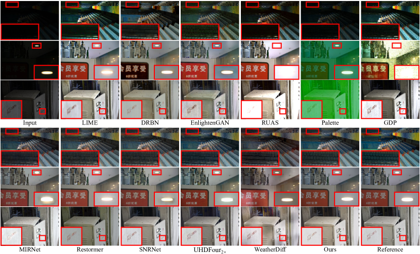
Figure 6. Qualitative comparison of our method and competitive methods on the LOLv1 (Wei et al., 2018) (row 1), LOLv2-real (Yang et al., 2021b) (row 2), and LSRW (Hai et al., 2023) (row 3) test sets. Error-prone regions are highlighted with red boxes, best viewed by zooming in.

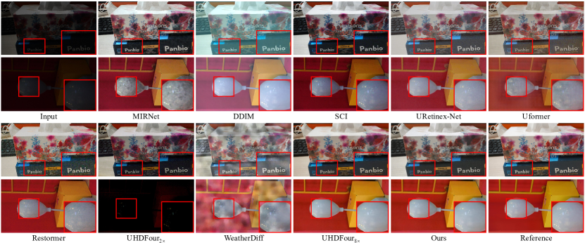
Figure 7. Qualitative comparison of our method and competitive methods on the UHD-LL (Li et al., 2023) test set. Error-prone regions are highlighted with red boxes, best viewed by zooming in. Note that UHDFour_8× is trained on the UHD-LL training set, while other comparison supervised methods and our method are trained on the simpler LOLv1 (Wei et al., 2018) training set.

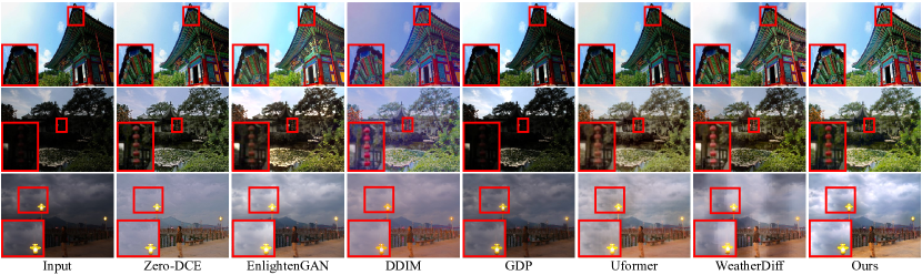
Figure 8. Qualitative comparison of our method and competitive methods on the DICM (Lee et al., 2013) (row 1), MEF (Ma et al., 2015) (row 2), and NPE (Wang et al., 2013) (row 3) datasets. Error-prone regions are highlighted with red boxes, best viewed by zooming in.

Moreover, we also compared the proposed DiffLL with competitive methods on five unpaired datasets to further validate the effectiveness of our method. Three non-reference perceptual metrics NIQE (Mittal et al., 2012b), BRISQUE (Mittal et al., 2012a), and PI (Blau et al., 2018) are utilized to evaluate the visual quality of the enhanced results, the lower the metrics the better the visual quality. As shown in Table 4, our method achieves the lowest NIQE score on the MEF, LIME, and NPE datasets, and is comparable to the best methods on the DICM and VV datasets. For BRISQUE and PI scores, we achieve the best results on four datasets as well as the second-best results on the remaining dataset. In summary, our method achieves the lowest average scores on all three metrics, which proves that our method has a better generalization ability to unseen real-world scenes.

Qualitative Comparison. We present qualitative comparisons of our method and state-of-the-art methods on the paired datasets in Fig. 6. The images in rows 1-3 are selected from LOLv1, LOLv2-real, and LSRW test sets, respectively. The results presented in rows 1 and 3 show that DRBN, MIRNet, RUAS, and GDP are unable to properly improve the contrast of the images, yielding underexposed or overexposed results. Likewise, EnlightenGAN suffers from noise amplification, while LIME, SNRNet, Restormer, UHDFour_2× and WeatherDiff produce over-smoothed textures and artifacts. Moreover, as depicted in row 2, the results restored by Palette and GDP are concomitant with chaotic content and color distortion, other methods typically introduce artifacts around the lamp, whereas WeatherDiff avoids this distortion in that particular area but exhibits artifacts elsewhere. In contrast, our method effectively improves global and local contrast, reconstructs sharper details, and suppresses noise, resulting in visually satisfactory results in all cases. The visual comparisons on the UHD-LL (Li et al., 2023) test set is illustrated in Fig. 7. As we can see that previous methods appear incorrect exposure, color distortion, noise amplification, or artifacts, thereby undermining the overall visual quality. In contrast, our method effectively improves global contrast and presents a vivid color without introducing chaotic content.

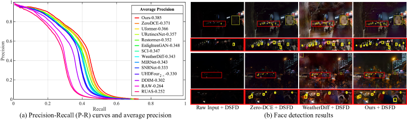
Figure 9. Comparison of face detection results before and after enhanced by different methods on the DARK FACE dataset (Yang et al., 2020b).

We also provide visual comparisons of our method and competitive methods on the unpaired datasets in Fig. 8, where the images in rows 1-3 are selected from DICM, MEF, and NPE datasets, respectively. The previous learning-based LLIE methods and GDP fail to relight the building and the lantern in rows 1 and 2 compared to our method and WeatherDiff, but WeatherDiff produces undesirable content in the sky. In row 3, Zero-DCE, EnlightenGAN, and DDIM smooth the cloud texture, as Uformer and WeatherDiff produce gridding effects and messy content. Our method successfully restores the illumination of the image and reconstructs the details, which demonstrates that our method can generalize well to unseen scenes. For more qualitative results, please refer to the supplementary material.

4.3. Low-Light Face Detection

In this section, we investigate the impact of LLIE methods as pre-processing on improving the face detection task under weakly illuminated conditions. Specifically, we take the DARK FACE dataset (Yang et al., 2020b) consisting of 10,000 images captured in real-world nighttime scenes for comparison, of which 6,000 images are selected as the training set, and the rest are adopted for testing. Since the bounding box labels of the test set are not publicly available, we utilize the training set for evaluation, applying our method and comparison methods as a pre-processing step, followed by the well-known learning-based face detector DSFD (Li et al., 2019). We illustrate the precision-recall (P-R) curves in Fig. 9(a) and compare the average precision (AP) under the IoU threshold of 0.5 using the official evaluation tool. As we can see that our proposed method achieves superior performance in the high recall area, and utilizing our approach as a pre-processing step leads to AP improvement from 26.4% to 38.5%. Observing the visual examples in Fig. 9(b), our method relights the face regions while maintaining well-illuminated regions, enabling DSFD more robust in weakly illuminated scenes.

4.4. Ablation Study

In this section, we conduct a set of ablation studies to measure the impact of different component configurations employed in our method. We employ the implementation details described in Sec. 4.1 to train all models and subsequently evaluate their performances on the LOLv1 (Wei et al., 2018) test set for analysis. Detailed experiment settings are discussed below.

Wavelet Transformation Scale. We first validate the impact of performing diffusion processes on the average coefficient at different wavelet scales $K$. As reported in Table 5, when we apply the WCDM to restore the average coefficient $A_{low}^{1}$, i.e., $K=1$, leads to overall performance improvements while resulting in the inference time increase. As the wavelet scale increases, the spatial dimension of the average coefficient decreases by $4^{K}$ relative to the original image, which causes performance degradation due to the information richness reduction but lowers the inference time. For a trade-off between performance and efficiency, we choose $K=2$ as the default setting. From another perspective, even if we perform three times wavelet transformation, i.e., $K=3$, our method is also comparable to the state-of-the-art methods reported in Table 1, which demonstrates that our proposed wavelet-based diffusion model can be applied to restore higher-resolution images.

Table 5. Ablation studies of various settings on the wavelet transformation scale and sampling step, please refer to the text for more details. The results using default settings are underlined.

Wavelet scale	Sampling step	PSNR $\uparrow$	SSIM $\uparrow$	LPIPS $\downarrow$	FID $\downarrow$	Time (s) $\downarrow$
$K=1$	$S=5$	26.256	0.855	0.188	40.884	0.198
	$S=10$	26.444	0.858	0.182	40.143	0.380
	$S=20$	26.385	0.856	0.179	40.001	0.757
	$S=30$	26.211	0.850	0.190	41.023	1.256
$K=2$	$S=5$	25.855	0.835	0.210	49.371	0.085
	$S=10$	26.336	0.845	0.217	48.114	0.157
	$S=20$	26.246	0.844	0.212	48.071	0.285
	$S=30$	26.094	0.851	0.213	49.993	0.477
$K=3$	$S=5$	24.408	0.817	0.283	61.234	0.066
	$S=10$	25.091	0.828	0.265	57.190	0.114
	$S=20$	25.103	0.826	0.271	57.227	0.237
	$S=30$	24.796	0.822	0.279	59.326	0.401

Sampling Step. Another factor that enables our method to be more computational efficiency is that a smaller sampling step $S$ is adopted. We present the performance of our method using different $S$ from 5 to 30 in Table 5. Benefiting from we conduct the denoising process during training, the model learns how to perform denoising with different steps, making variations in sampling steps, whether smaller or larger, have no major impact on the performance of our proposed WCDM. A large sampling step contributes to generating images with better visual quality for diffusion-based image generation methods (Ho et al., 2020; Song et al., 2021a), while for us it only increases the inference time, which indicates that larger sampling steps, e.g., $S=1000$ in GDP (Fei et al., 2023) and Palette (Saharia et al., 2022), may not be essential for diffusion-based LLIE and other relative image restoration tasks using our proposed framework.

High-frequency Restoration Module. To validate the effectiveness of our designed high-frequency restoration module (HFRM), we form a baseline by using the proposed wavelet-based conditional diffusion model (WCDM) only to restore the average coefficient. As shown in rows 1-3 of Table 6, the HFRMs utilized to reconstruct the high-frequency coefficients at wavelet scales $k=1$ and $k=2$ improve the overall performance, achieving 2.142dB and 1.440dB gains in terms of PSNR, as well as 0.064 and 0.044 in terms of SSIM, respectively. Since the high-frequency coefficients at $k=1$ have richer details than the coefficients at $k=2$, the HFRM₁ is thus capable of delivering greater gains. Furthermore, we have formed two HFRM versions dubbed HFRM-v2 and HFRM-v3 to explore the effect of high-frequency coefficients complementarity. Specifically, the HFRM-v2 does not leverage the information in vertical and horizontal directions to complement the details present in the diagonal by using convolutional layers with equal parameters to replace cross-attention layers. On the other hand, the HFRM-v3 utilizes information from the diagonal direction to reinforce the vertical and horizontal details. As reported in rows 4-6 of Table 6, our default HFRM is superior to the other two versions, which demonstrates the effectiveness of high-frequency complementarity and that complementing diagonal details with information in vertical and horizontal directions being more useful than the reverse.

Table 6. Ablation studies of the effectiveness of our high-frequency restoration module. The results using default settings are underlined.

	PSNR $\uparrow$	SSIM $\uparrow$	LPIPS $\downarrow$	FID $\downarrow$
WCDM	21.975	0.729	0.310	98.104
WCDM + HFRM2	23.415	0.773	0.259	76.193
WCDM + HFRM1	24.117	0.793	0.251	62.210
WCDM + HFRM-v2	24.145	0.822	0.266	67.909
WCDM + HFRM-v3	25.630	0.824	0.221	51.466
Default	26.336	0.845	0.217	48.114

Table 7. Ablation studies of the loss function terms. The results using default settings are underlined. ‘w/o’ denotes without.

	PSNR $\uparrow$	SSIM $\uparrow$	LPIPS $\downarrow$	FID $\downarrow$
w/o $\mathcal{L}_{diff}$	24.238	0.823	0.314	89.318
w/o $\mathcal{L}_{content}$	23.821	0.808	0.283	67.502
w/o $\mathcal{L}_{detail}$	25.413	0.835	0.249	57.663
vanilla $\mathcal{L}_{diff}$ (Eq.8)	25.956	0.838	0.221	50.467
Default	26.306	0.845	0.217	48.114

Loss Function. To validate the effectiveness of the proposed loss functions, we conduct experiments by individually removing each component from the default setting, where the quantitative results are reported in Table 7. As shown in row 1, the removal of the diffusion loss $\mathcal{L}_{diff}$ results in decreases in all perceptual metrics, as the generative capacity of diffusion models relies heavily on this component. The incorporation of content loss $\mathcal{L}_{content}$ yields noticeable improvements, especially the distortion metrics, which can be improved by 2.485dB and 0.037 for PSNR and SSIM, respectively, as shown in row 2 and row 5. The detail preserve loss $\mathcal{L}_{detail}$ is designed to reconstruct more image details, thus its removal causes performance degradation. However, such degradation is not significant relative to removing the content loss, which reveals the importance of the content loss. From another perspective, the content loss should be integrated with our proposed training strategy, which also illustrates its effectiveness. Furthermore, as described in Sec. 3.3, we incorporate an extra loss term into the vanilla diffusion loss, i.e., Eq.8, to promote the restoration of the average coefficient. To validate the effectiveness of the auxiliary term, we employ vanilla diffusion loss to optimize the noise estimator network. As shown in row 4, the inclusion of the auxiliary term proves to be beneficial in enhancing the visual fidelity of the restored images, thereby leading to the overall performance improved.

Table 8. Ablation studies of the training strategy of our wavelet-based conditional diffusion model. The results using default settings are underlined.

Methods	PSNR $\uparrow$	SSIM $\uparrow$	LPIPS $\downarrow$	FID $\downarrow$
DDIM∗	16.521±0.544	0.776±0.002	0.376±0.001	84.071${{}_{\pm}32.909}$
Palette∗	11.771±0.254	0.561±0.001	0.498±0.001	108.291${{}_{\pm}8.019}$
WeatherDiff∗	17.913±0.182	0.811±0.001	0.272±0.001	73.903${{}_{\pm}5.265}$
Ours${}_{\operatorname{FD}}$	18.125±0.212	0.789±0.001	0.273±0.002	64.676±5.544
Ours${}_{\operatorname{FD+DP}}$	26.336${}_{\pm 1\times 10^{-5}}$	0.845${}_{\pm 2\times 10^{-7}}$	0.217${}_{\pm 6\times 10^{-9}}$	48.114±0.006

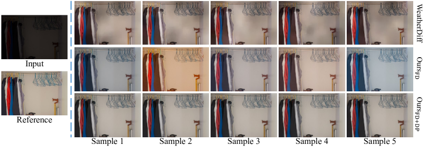
Figure 10. The sampling results from five evaluations, in which performing forward diffusion only in the training phase results in diverse outputs, while our training strategy contributes to generating results with consistency.

Training Strategy. The content diversity caused by randomly sampled noise during the denoising process of diffusion models is undesirable for some image restoration tasks, such as LLIE, dehazing, deraining, etc. As described in Sec. 3.3, we address this issue by incorporating the denoising process (DP) in both training and inference phases to achieve consistency. As shown in Table 8, we report the means and variances of five evaluations for three diffusion-based methods, our method that performs forward diffusion (FD) only in the training phase denoted as Ours${}_{\operatorname{FD}}$, and our method with the default training strategy denoted as Ours${}_{\operatorname{FD+DP}}$. By incorporating DP into the training phase, our method not only achieves the best performance but also aids in circumventing content diversity and yields minimal variance, which proves the superiority of our training strategy. The restored results of five evaluations illustrated in Fig. 10 show that performing forward diffusion only in the training phase leads to diverse results, while our default training strategy not only mitigates the appearance of chaotic content and color distortion but also facilitates generating images with consistency.

4.5. Limitations

Although our method is effective in restoring images captured in weakly illuminated conditions, it does not work as well in extremely low-light environments as images captured in such conditions suffer from greater information loss and are more challenging to restore. In addition, some real-time methods can be applied directly to the low-light video enhancement task, whereas our method is not yet efficient enough to be applied directly to this task. Another natural limitation of our model is its inherently limited capacity to only generalize to the LLIE task observed at training time, and investigating the effectiveness of the proposed approach for other image restoration tasks will be our future work.

5. Conclusions

We have presented DiffLL, a diffusion-based framework for robust and efficient low-light image enhancement. Technically, we propose a wavelet-based conditional diffusion model that leverages the generative ability of diffusion models and wavelet transformation to produce visually satisfactory results while reducing inference time and computational resource consumption. Moreover, to circumvent content diversity during inference, we perform the denoising process in both the training and inference phases, enabling the model to learn stable sampling and obtain restored results with consistency. Additionally, we design a high-frequency restoration module to complement the diagonal details with vertical and horizontal information for better fine-grained details reconstruction. Experimental results on publicly available benchmarks demonstrate that our method outperforms competitors both quantitatively and qualitatively while being computationally efficient. The results of the low-light face detection also show the practical values of our method.

References

- (1)
- Blau et al. (2018) Yochai Blau, Roey Mechrez, Radu Timofte, Tomer Michaeli, and Lihi Zelnik-Manor. 2018. The 2018 PIRM challenge on perceptual image super-resolution. In European Conference on Computer Vision.
- Bovik (2010) Alan C Bovik. 2010. Handbook of image and video processing. Academic press.
- Chan et al. (2011) Stanley H Chan, Ramsin Khoshabeh, Kristofor B Gibson, Philip E Gill, and Truong Q Nguyen. 2011. An augmented Lagrangian method for total variation video restoration. IEEE Transactions on Image Processing 20, 11 (2011), 3097–3111.
- Chollet (2017) François Chollet. 2017. Xception: Deep learning with depthwise separable convolutions. In Proceedings of the IEEE/CVF Conference on Computer Vision and Pattern Recognition. 1251–1258.
- Chung et al. (2022) Hyungjin Chung, Byeongsu Sim, and Jong Chul Ye. 2022. Come-closer-diffuse-faster: Accelerating conditional diffusion models for inverse problems through stochastic contraction. In Proceedings of the IEEE/CVF Conference on Computer Vision and Pattern Recognition. 12413–12422.
- Dabov et al. (2007) Kostadin Dabov, Alessandro Foi, Vladimir Katkovnik, and Karen Egiazarian. 2007. Image denoising by sparse 3-D transform-domain collaborative filtering. IEEE Transactions on Image Processing 16, 8 (2007), 2080–2095.
- Dong et al. (2015) Chao Dong, Chen Change Loy, Kaiming He, and Xiaoou Tang. 2015. Image super-resolution using deep convolutional networks. IEEE transactions on pattern analysis and machine intelligence 38, 2 (2015), 295–307.
- Fei et al. (2023) Ben Fei, Zhaoyang Lyu, Liang Pan, Junzhe Zhang, Weidong Yang, Tianyue Luo, Bo Zhang, and Bo Dai. 2023. Generative Diffusion Prior for Unified Image Restoration and Enhancement. In Proceedings of the IEEE/CVF Conference on Computer Vision and Pattern Recognition. 9935–9946.
- Fu et al. (2016) Xueyang Fu, Delu Zeng, Yue Huang, Xiao-Ping Zhang, and Xinghao Ding. 2016. A weighted variational model for simultaneous reflectance and illumination estimation. In Proceedings of the IEEE/CVF Conference on Computer Vision and Pattern Recognition. 2782–2790.
- Guo et al. (2020) Chunle Guo, Chongyi Li, Jichang Guo, Chen Change Loy, Junhui Hou, Sam Kwong, and Runmin Cong. 2020. Zero-reference deep curve estimation for low-light image enhancement. In Proceedings of the IEEE/CVF Conference on Computer Vision and Pattern Recognition. 1780–1789.
- Guo et al. (2023) Lanqing Guo, Chong Wang, Wenhan Yang, Siyu Huang, Yufei Wang, Hanspeter Pfister, and Bihan Wen. 2023. Shadowdiffusion: When degradation prior meets diffusion model for shadow removal. In Proceedings of the IEEE/CVF Conference on Computer Vision and Pattern Recognition. 14049–14058.
- Guo et al. (2016) Xiaojie Guo, Yu Li, and Haibin Ling. 2016. LIME: Low-light image enhancement via illumination map estimation. IEEE Transactions on Image Processing 26, 2 (2016), 982–993.
- Haar (1911) Alfred Haar. 1911. Zur theorie der orthogonalen funktionensysteme. Math. Ann. 71, 1 (1911), 38–53.
- Hai et al. (2021) Jiang Hai, Yutong Hao, Fengzhu Zou, Fang Lin, and Songchen Han. 2021. A Visual Navigation System for UAV under Diverse Illumination Conditions. Applied Artificial Intelligence 35, 15 (2021), 1529–1549.
- Hai et al. (2023) Jiang Hai, Zhu Xuan, Ren Yang, Yutong Hao, Fengzhu Zou, Fang Lin, and Songchen Han. 2023. R2rnet: Low-light image enhancement via real-low to real-normal network. Journal of Visual Communication and Image Representation 90 (2023), 103712.
- Hai et al. (2022) Jiang Hai, Ren Yang, Yaqi Yu, and Songchen Han. 2022. Combining Spatial and Frequency Information for Image Deblurring. IEEE Signal Processing Letters 29 (2022), 1679–1683.
- Heusel et al. (2017) Martin Heusel, Hubert Ramsauer, Thomas Unterthiner, Bernhard Nessler, and Sepp Hochreiter. 2017. Gans trained by a two time-scale update rule converge to a local nash equilibrium. Advances in Neural Information Processing Systems 30 (2017).
- Ho et al. (2020) Jonathan Ho, Ajay Jain, and Pieter Abbeel. 2020. Denoising diffusion probabilistic models. Advances in Neural Information Processing Systems 33 (2020), 6840–6851.
- Hou et al. (2019) Ruibing Hou, Hong Chang, Bingpeng Ma, Shiguang Shan, and Xilin Chen. 2019. Cross attention network for few-shot classification. Advances in Neural Information Processing Systems 32 (2019).
- Jiang et al. (2021) Yifan Jiang, Xinyu Gong, Ding Liu, Yu Cheng, Chen Fang, Xiaohui Shen, Jianchao Yang, Pan Zhou, and Zhangyang Wang. 2021. Enlightengan: Deep light enhancement without paired supervision. IEEE Transactions on Image Processing 30 (2021), 2340–2349.
- Jobson et al. (1997) Daniel J Jobson, Zia-ur Rahman, and Glenn A Woodell. 1997. A multiscale retinex for bridging the gap between color images and the human observation of scenes. IEEE Transactions on Image processing 6, 7 (1997), 965–976.
- Johnson et al. (2016) Justin Johnson, Alexandre Alahi, and Li Fei-Fei. 2016. Perceptual losses for real-time style transfer and super-resolution. In European Conference on Computer Vision. 694–711.
- Kawar et al. (2022) Bahjat Kawar, Michael Elad, Stefano Ermon, and Jiaming Song. 2022. Denoising diffusion restoration models. Advances in Neural Information Processing Systems 35 (2022), 23593–23606.
- Kingma and Ba (2015) Diederik P Kingma and Jimmy Ba. 2015. Adam: A Method for Stochastic Optimization. In International Conference on Learning Representations.
- Land (1977) Edwin H Land. 1977. The retinex theory of color vision. Scientific American 237, 6 (1977), 108–129.
- Lee et al. (2013) Chulwoo Lee, Chul Lee, and Chang-Su Kim. 2013. Contrast enhancement based on layered difference representation of 2D histograms. IEEE transactions on Image Processing 22, 12 (2013), 5372–5384.
- Lei et al. (2022) Xiaozhou Lei, Zixiang Fei, Wenju Zhou, Huiyu Zhou, and Minrui Fei. 2022. Low-light Image Enhancement Using the Cell Vibration Model. IEEE Transactions on Multimedia (2022).
- Li et al. (2021a) Chongyi Li, Chunle Guo, Linghao Han, Jun Jiang, Ming-Ming Cheng, Jinwei Gu, and Chen Change Loy. 2021a. Low-light image and video enhancement using deep learning: A survey. IEEE Transactions on Pattern Analysis and Machine Intelligence 44, 12 (2021), 9396–9416.
- Li et al. (2023) Chongyi Li, Chun-Le Guo, Man Zhou, Zhexin Liang, Shangchen Zhou, Ruicheng Feng, and Chen Change Loy. 2023. Embedding Fourier for Ultra-High-Definition Low-Light Image Enhancement. In International Conference on Learning Representations.
- Li et al. (2021c) Guofa Li, Yifan Yang, Xingda Qu, Dongpu Cao, and Keqiang Li. 2021c. A deep learning based image enhancement approach for autonomous driving at night. Knowledge-Based Systems 213 (2021), 106617.
- Li et al. (2021b) Jichun Li, Weimin Tan, and Bo Yan. 2021b. Perceptual variousness motion deblurring with light global context refinement. In Proceedings of the IEEE/CVF International Conference on Computer Vision. 4116–4125.
- Li et al. (2019) Jian Li, Yabiao Wang, Changan Wang, Ying Tai, Jianjun Qian, Jian Yang, Chengjie Wang, Jilin Li, and Feiyue Huang. 2019. DSFD: dual shot face detector. In Proceedings of the IEEE/CVF Conference on Computer Vision and Pattern Recognition. 5060–5069.
- Li et al. (2022) Youwei Li, Haibin Huang, Lanpeng Jia, Haoqiang Fan, and Shuaicheng Liu. 2022. D2C-SR: A Divergence to Convergence Approach for Real-World Image Super-Resolution. In European Conference on Computer Vision. 379–394.
- Liang et al. (2021) Jinxiu Liang, Jingwen Wang, Yuhui Quan, Tianyi Chen, Jiaying Liu, Haibin Ling, and Yong Xu. 2021. Recurrent exposure generation for low-light face detection. IEEE Transactions on Multimedia 24 (2021), 1609–1621.
- Lim and Kim (2020) Seokjae Lim and Wonjun Kim. 2020. DSLR: deep stacked Laplacian restorer for low-light image enhancement. IEEE Transactions on Multimedia 23 (2020), 4272–4284.
- Lin and Shi (2014) Haoning Lin and Zhenwei Shi. 2014. Multi-scale retinex improvement for nighttime image enhancement. optik 125, 24 (2014), 7143–7148.
- Liu et al. (2021) Risheng Liu, Long Ma, Jiaao Zhang, Xin Fan, and Zhongxuan Luo. 2021. Retinex-inspired unrolling with cooperative prior architecture search for low-light image enhancement. In Proceedings of the IEEE/CVF Conference on Computer Vision and Pattern Recognition. 10561–10570.
- Loh and Chan (2019) Yuen Peng Loh and Chee Seng Chan. 2019. Getting to know low-light images with the exclusively dark dataset. Computer Vision and Image Understanding 178 (2019), 30–42.
- Lore et al. (2017) Kin Gwn Lore, Adedotun Akintayo, and Soumik Sarkar. 2017. LLNet: A deep autoencoder approach to natural low-light image enhancement. Pattern Recognition 61 (2017), 650–662.
- Lugmayr et al. (2022) Andreas Lugmayr, Martin Danelljan, Andres Romero, Fisher Yu, Radu Timofte, and Luc Van Gool. 2022. Repaint: Inpainting using denoising diffusion probabilistic models. In Proceedings of the IEEE/CVF Conference on Computer Vision and Pattern Recognition. 11461–11471.
- Luo et al. (2023a) Ziwei Luo, Fredrik K Gustafsson, Zheng Zhao, Jens Sjölund, and Thomas B Schön. 2023a. Image Restoration with Mean-Reverting Stochastic Differential Equations. arXiv preprint arXiv:2301.11699 (2023).
- Luo et al. (2023b) Ziwei Luo, Fredrik K Gustafsson, Zheng Zhao, Jens Sjölund, and Thomas B Schön. 2023b. Refusion: Enabling large-size realistic image restoration with latent-space diffusion models. In Proceedings of the IEEE/CVF Conference on Computer Vision and Pattern Recognition Workshops. 1680–1691.
- Ma et al. (2015) Kede Ma, Kai Zeng, and Zhou Wang. 2015. Perceptual quality assessment for multi-exposure image fusion. IEEE Transactions on Image Processing 24, 11 (2015), 3345–3356.
- Ma et al. (2022) Long Ma, Tengyu Ma, Risheng Liu, Xin Fan, and Zhongxuan Luo. 2022. Toward Fast, Flexible, and Robust Low-Light Image Enhancement. In Proceedings of the IEEE/CVF Conference on Computer Vision and Pattern Recognition. 5637–5646.
- Mao et al. (2016) Xiaojiao Mao, Chunhua Shen, and Yu-Bin Yang. 2016. Image restoration using very deep convolutional encoder-decoder networks with symmetric skip connections. Advances in Neural Information Processing Systems 29 (2016).
- Mittal et al. (2012a) Anish Mittal, Anush Krishna Moorthy, and Alan Conrad Bovik. 2012a. No-reference image quality assessment in the spatial domain. IEEE Transactions on image processing 21, 12 (2012), 4695–4708.
- Mittal et al. (2012b) Anish Mittal, Rajiv Soundararajan, and Alan C Bovik. 2012b. Making a “completely blind” image quality analyzer. IEEE Signal Processing Letters 20, 3 (2012), 209–212.
- Ooi and Isa (2010) Chen Hee Ooi and Nor Ashidi Mat Isa. 2010. Quadrants dynamic histogram equalization for contrast enhancement. IEEE Transactions on Consumer Electronics 56, 4 (2010), 2552–2559.
- Özdenizci and Legenstein (2023) Ozan Özdenizci and Robert Legenstein. 2023. Restoring vision in adverse weather conditions with patch-based denoising diffusion models. IEEE Transactions on Pattern Analysis and Machine Intelligence 45, 8 (2023), 10346–10357.
- Park et al. (2022) Jaemin Park, An Gia Vien, Jin-Hwan Kim, and Chul Lee. 2022. Histogram-Based Transformation Function Estimation for Low-Light Image Enhancement. In IEEE International Conference on Image Processing. IEEE, 1–5.
- Peng et al. (2021) Jialun Peng, Dong Liu, Songcen Xu, and Houqiang Li. 2021. Generating diverse structure for image inpainting with hierarchical VQ-VAE. In Proceedings of the IEEE/CVF Conference on Computer Vision and Pattern Recognition. 10775–10784.
- Ren et al. (2022) Mengwei Ren, Mauricio Delbracio, Hossein Talebi, Guido Gerig, and Peyman Milanfar. 2022. Image Deblurring with Domain Generalizable Diffusion Models. arXiv preprint arXiv:2212.01789 (2022).
- Rombach et al. (2022) Robin Rombach, Andreas Blattmann, Dominik Lorenz, Patrick Esser, and Björn Ommer. 2022. High-resolution image synthesis with latent diffusion models. In Proceedings of the IEEE/CVF Conference on Computer Vision and Pattern Recognition. 10684–10695.
- Ronneberger et al. (2015) Olaf Ronneberger, Philipp Fischer, and Thomas Brox. 2015. U-net: Convolutional networks for biomedical image segmentation. In Proceedings of the International Conference on Medical Image Computing and Computer-Assisted Intervention. 234–241.
- Saharia et al. (2022) Chitwan Saharia, William Chan, Huiwen Chang, Chris Lee, Jonathan Ho, Tim Salimans, David Fleet, and Mohammad Norouzi. 2022. Palette: Image-to-image diffusion models. In ACM SIGGRAPH 2022 Conference Proceedings. 1–10.
- Shang et al. (2023) Shuyao Shang, Zhengyang Shan, Guangxing Liu, and Jinglin Zhang. 2023. ResDiff: Combining CNN and Diffusion Model for Image Super-Resolution. arXiv preprint arXiv:2303.08714 (2023).
- Singh et al. (2015) Kuldeep Singh, Rajiv Kapoor, and Sanjeev Kr Sinha. 2015. Enhancement of low exposure images via recursive histogram equalization algorithms. Optik 126, 20 (2015), 2619–2625.
- Sohl-Dickstein et al. (2015) Jascha Sohl-Dickstein, Eric Weiss, Niru Maheswaranathan, and Surya Ganguli. 2015. Deep unsupervised learning using nonequilibrium thermodynamics. In International Conference on Machine Learning. 2256–2265.
- Song et al. (2021a) Jiaming Song, Chenlin Meng, and Stefano Ermon. 2021a. Denoising Diffusion Implicit Models. In International Conference on Learning Representations.
- Song and Ermon (2019) Yang Song and Stefano Ermon. 2019. Generative modeling by estimating gradients of the data distribution. Advances in Neural Information Processing Systems 32 (2019).
- Song et al. (2021b) Yang Song, Jascha Sohl-Dickstein, Diederik P Kingma, Abhishek Kumar, Stefano Ermon, and Ben Poole. 2021b. Score-Based Generative Modeling through Stochastic Differential Equations. In International Conference on Learning Representations.
- Sun et al. (2015) Jian Sun, Wenfei Cao, Zongben Xu, and Jean Ponce. 2015. Learning a convolutional neural network for non-uniform motion blur removal. In Proceedings of the IEEE/CVF Conference on Computer Vision and Pattern Recognition. 769–777.
- Wang et al. (2013) Shuhang Wang, Jin Zheng, Hai-Miao Hu, and Bo Li. 2013. Naturalness preserved enhancement algorithm for non-uniform illumination images. IEEE Transactions on Image Processing 22, 9 (2013), 3538–3548.
- Wang et al. (2004) Zhou Wang, A.C. Bovik, H.R. Sheikh, and E.P. Simoncelli. 2004. Image quality assessment: from error visibility to structural similarity. IEEE Transactions on Image Processing 13, 4 (2004), 600–612.
- Wang et al. (2022) Zhendong Wang, Xiaodong Cun, Jianmin Bao, Wengang Zhou, Jianzhuang Liu, and Houqiang Li. 2022. Uformer: A general u-shaped transformer for image restoration. In Proceedings of the IEEE/CVF Conference on Computer Vision and Pattern Recognition. 17683–17693.
- Wang et al. (2023) Zhixin Wang, Xiaoyun Zhang, Ziying Zhang, Huangjie Zheng, Mingyuan Zhou, Ya Zhang, and Yanfeng Wang. 2023. DR2: Diffusion-based Robust Degradation Remover for Blind Face Restoration. In Proceedings of the IEEE/CVF Conference on Computer Vision and Pattern Recognition. 1704–1713.
- Wei et al. (2018) Chen Wei, Wenjing Wang, Wenhan Yang, and Jiaying Liu. 2018. Deep Retinex Decomposition for Low-Light Enhancement. In British Machine Vision Conference.
- Wu et al. (2022) Wenhui Wu, Jian Weng, Pingping Zhang, Xu Wang, Wenhan Yang, and Jianmin Jiang. 2022. Uretinex-net: Retinex-based deep unfolding network for low-light image enhancement. In Proceedings of the IEEE/CVF Conference on Computer Vision and Pattern Recognition. 5901–5910.
- Xu et al. (2022) Xiaogang Xu, Ruixing Wang, Chi-Wing Fu, and Jiaya Jia. 2022. SNR-aware low-light image enhancement. In Proceedings of the IEEE/CVF Conference on Computer Vision and Pattern Recognition. 17714–17724.
- Yang et al. (2022) Shaoliang Yang, Dongming Zhou, Jinde Cao, and Yanbu Guo. 2022. Rethinking low-light enhancement via transformer-GAN. IEEE Signal Processing Letters 29 (2022), 1082–1086.
- Yang et al. (2021a) Tao Yang, Peiran Ren, Xuansong Xie, and Lei Zhang. 2021a. Gan prior embedded network for blind face restoration in the wild. In Proceedings of the IEEE/CVF Conference on Computer Vision and Pattern Recognition. 672–681.
- Yang et al. (2020a) Wenhan Yang, Shiqi Wang, Yuming Fang, Yue Wang, and Jiaying Liu. 2020a. From fidelity to perceptual quality: A semi-supervised approach for low-light image enhancement. In Proceedings of the IEEE/CVF Conference on Computer Vision and Pattern Recognition. 3063–3072.
- Yang et al. (2021b) Wenhan Yang, Wenjing Wang, Haofeng Huang, Shiqi Wang, and Jiaying Liu. 2021b. Sparse gradient regularized deep retinex network for robust low-light image enhancement. IEEE Transactions on Image Processing 30 (2021), 2072–2086.
- Yang et al. (2020b) Wenhan Yang, Ye Yuan, Wenqi Ren, Jiaying Liu, Walter J Scheirer, Zhangyang Wang, Taiheng Zhang, Qiaoyong Zhong, Di Xie, Shiliang Pu, et al. 2020b. Advancing image understanding in poor visibility environments: A collective benchmark study. IEEE Transactions on Image Processing 29 (2020), 5737–5752.
- Zamir et al. (2022) Syed Waqas Zamir, Aditya Arora, Salman Khan, Munawar Hayat, Fahad Shahbaz Khan, and Ming-Hsuan Yang. 2022. Restormer: Efficient transformer for high-resolution image restoration. In Proceedings of the IEEE/CVF Conference on Computer Vision and Pattern Recognition. 5728–5739.
- Zamir et al. (2020) Syed Waqas Zamir, Aditya Arora, Salman Khan, Munawar Hayat, Fahad Shahbaz Khan, Ming-Hsuan Yang, and Ling Shao. 2020. Learning enriched features for real image restoration and enhancement. In European Conference on Computer Vision. 492–511.
- Zhang et al. (2021) Rongkai Zhang, Lanqing Guo, Siyu Huang, and Bihan Wen. 2021. Rellie: Deep reinforcement learning for customized low-light image enhancement. In Proceedings of the 29th ACM International Conference on Multimedia. 2429–2437.
- Zhang et al. (2018) Richard Zhang, Phillip Isola, Alexei A Efros, Eli Shechtman, and Oliver Wang. 2018. The unreasonable effectiveness of deep features as a perceptual metric. In Proceedings of the IEEE/CVF Conference on Computer Vision and Pattern Recognition. 586–595.
- Zheng et al. (2022) Dihan Zheng, Xiaowen Zhang, Kaisheng Ma, and Chenglong Bao. 2022. Learn from unpaired data for image restoration: A variational bayes approach. IEEE Transactions on Pattern Analysis and Machine Intelligence 45, 5 (2022), 5889–5903.