A fast and accurate computation method for reflective diffraction simulations

Abstract

We present a new computation method for simulating reflection high-energy electron diffraction and the total-reflection high-energy positron diffraction experiments. The two experiments are used commonly for the structural analysis of material surface. The present paper improves the conventional numerical method, the multi-slice method, for faster computation, since the present method avoids the matrix-eigenvalue solver for the computation of matrix exponentials and can adopt higher-order ordinary differential equation solvers. Moreover, we propose a high-performance implementation based on multi-thread parallelization and cache-reusable subroutines. In our tests, this new method performs up to 2,000 times faster than the conventional method.

[uec]organization=The University of Electro-Communications, addressline=1-5-1 Chofugaoka, city=Chofu, postcode=182-8585, country=Japan [tottori]organization=Tottori University, addressline=4-101 Koyama-cho Minami, city=Tottori, postcode=680-8550, country=Japan

1 Introduction

Nowadays, fast and accurate numerical methods are of great importance for data-driven science, in particular, for a global search analysis. As a typical problem, an equation is characterized by a parameter set $\bm{x}=(x^{(1)},x^{(2)},..,x^{(n)})$ and one should solve the equation numerically on many different points in the parameter space of $\bm{x}$. A major application field in computational physics is the reverse analysis of experimental measurement, in which the observed data $\bm{d}$ can be described as a function of the target quantity $\bm{x}$ ($\bm{d}_{\mathrm{cal}}=f(\bm{x})$). Hereinafter, the function $f$ is called the forward model. A typical approach is an optimization analysis in which the optimal value of the target quantity $\bm{x}^{*}=\operatorname*{argmin}_{\bm{x}}|\bm{d}-F(\bm{x})|^{2}$ is computed by a global optimization method, such as a grid search or Bayesian optimization. Another typical approach is Bayesian inference, in which the posterior priority density $P(\bm{x}|\bm{d})$ is obtained as a histogram. These approaches require the computation of $f(\bm{x})$ for a large dataset of $\bm{x}=\bm{x}_{1},\bm{x}_{2},\ldots$. Among such approaches, a rapid numerical computation is desired for performing reverse analysis with a larger dataset.

The present paper is motivated by the reverse analysis of the two experimental measurements, reflection high-energy electron diffraction (RHEED) [1] and total-reflection high-energy positron diffraction (TRHEPD) [2, 3]. RHEED and TRHEPD are experimental probes for crystal surface structures, i.e., positions of the atoms $\bm{x}$ in the surface and subsurface atomic layers. In RHEED and TRHEPD, quantum beams of electrons and positrons, respectively, are irradiated to the crystal surface and observe the diffraction patterns of the reflected waves $\bm{d}$. TRHEPD is more sensitive to the shallower layers of the surface than RHEED. There is an open-source RHEED/TRHEPD simulation software sim-trhepd-rheed [4, 5], which is used for many data analysis of surface structures based of RHEED [6, 7, 8, 9, 10, 11, 12, 13, 14, 15, 16, 17, 18, 19] and TRHEPD [20, 21, 22, 23, 24, 25]. Motoyama et.al. [23] demonstrated the reverse analysis of TRHEPD using their fully automated software 2DMAT that enable us the global search algorithms. In several global search algorithms, the forward problems with many points of the parameter space of $\bm{x}=\bm{x}_{1},\bm{x}_{2},\ldots$ are solved simultaneously as a parallel computation.

The present standard method for performing a forward computation of RHEED/TRHEPD is the multi-slice method [26, 1]. The multi-slice method solves the stationary Schrödinger equation as a boundary value problem (BVP) by expanding the wave function with periodic functions in the x-y plane and obtaining ordinary differential equations (ODEs) for the z-axis. The range of $z$ is divided into thin slices of size $h$ and the potential $v(z)$ is approximated by a constant matrix $A_{i}$ in each slice. Thus, the matrix exponential $\hat{A}_{i}=\mathrm{e}^{hA_{i}}$ becomes the transfer matrix of each slice $i$, and their product $\hat{A}_{0}\hat{A}_{1}\cdots$ becomes that of the whole crystal. To solve this, Ichimiya invented a technique that we call the recursive reflection technique. The technique solves the matrix eigenvalue problem for the calculation of matrix exponential $A_{i}$ on each slice, which will be costly, when the matrix dimension of $A_{i}$ increases. The computational cost is proportional to the number of the slices $N_{\rm slice}$ and, thus, to the inverse of slice size $h$.

We propose a new fast computation method by reorganizing the problem as a matrix ODE and improving the recursive reflection technique in higher-order ODE solver algorithms. The present method realizes fast and accurate numerical computation, because the present method does not require a matrix-eigenvalue problem and the slice size $h$ can be chosen to be more than $10$ fold larger than the original one to achieve the same accuracy. Furthermore, we propose a high-performance implementation method based on the implementation techniques in the highe-performance computing (HPC), such as multi-thread parallelization and the active use of cache-reusable subroutines, to exploit the performance of recent CPUs. As a result, our method performs up to $2,000$ times faster than the implementation of the conventional method in our tests. Although we apply our new method only to RHEED/TRHEPD simulation in this study, this method can potentially be extended to other many-beam reflective diffraction simulations.

Table 1: List of notations used in this paper

Symbol	Description
$\mathrm{i}$	the imaginary unit
$\mathrm{e}$	the Euler’s number
$\bm{a}$	vectors
$(\bm{a})_{i}$	the $i$-th component of the vector $\bm{a}$.
$A$	matrices
$(A)_{i,j}$	the $(i,j)$ component of the matrix $A$
$I_{n}$	the identity matrix of size $n\times n$
$O_{n}$	the zero matrix of size $n\times n$
$\hat{X}$	numerical approximations of quantity $X$

We summarize the notations used in this article in Table 1.

The reminder of the article is organized as follows. In Section 2, we introduce the simulation model of RHEED/TRHEPD and summarize the conventional computation technique developed by Ichimiya [26]. In Section 3, we describe our proposed method, and we compare the performance of our proposed method with that of the conventional implementation in Section 5. We present our discussions and conclusions in Section 6 and 7.

2 Simulation technique for RHEED/TRHEPD

2.1 Numerical problem

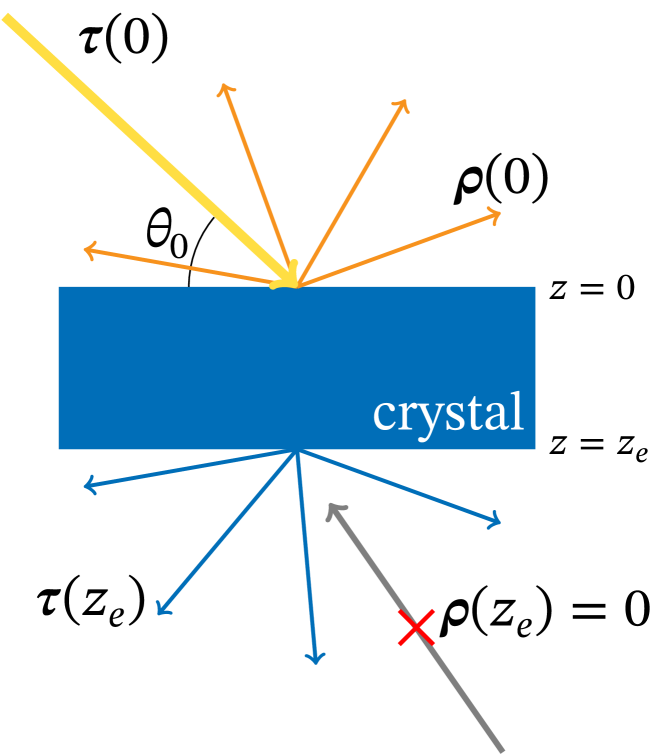
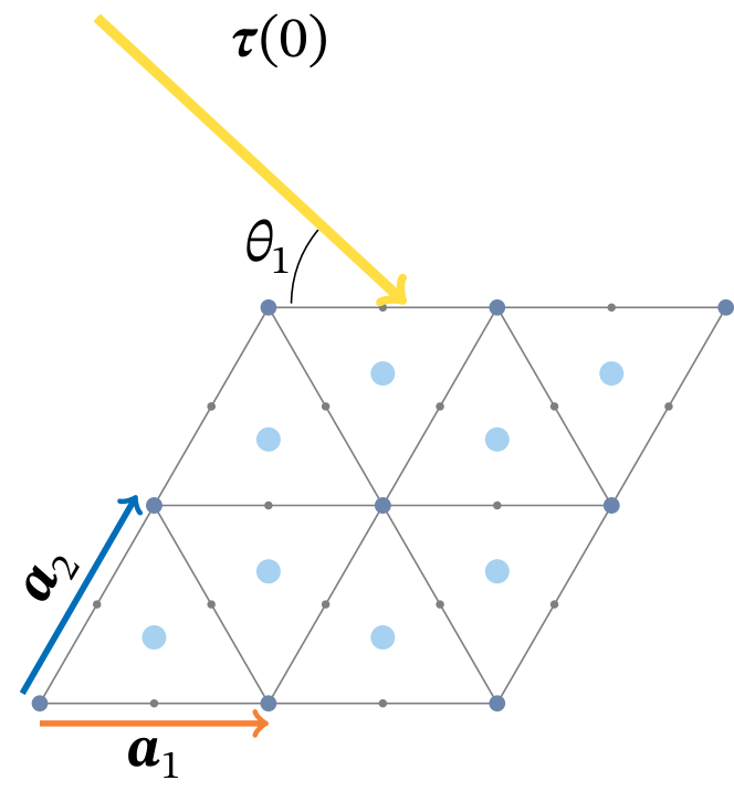
Figure 1: Left: Illustration of the boundary conditions of the computational system, a shallow surface region of crystal. $\theta_{0}$ is the altitude of the incident wave $\bm{\tau}(0)$. Right: Illustration of the lattice structure of the crystal surface ($z=0$) from the top. $\theta_{1}$ is the azimuth of $\bm{\tau}(0)$.

Here, we introduce the numerical method for RHEED developped by Ichimiya [26, 1] and TRHEPD  [2]. The computational system is a shallow surface region of crystal, as shown in Fig. 1. The coordinate axes are set so that the material surface is parallel to the x-y plane at precisely $z=0$, and the position of the bottom boundary of the system is $z=z_{\text{e}}$. The positions of the atoms are two-dimensionally periodic parallel to the x-y plane, but not periodic along the z-axis.

Let us assume that the incident wave and reflection wave satisfy the stationary Schrödinger equation:

$$\left(\Delta+\gamma^{2}+v(\bm{r})\right)\psi(\bm{r})=0,$$ (1)

where $\bm{r}$ is the position, $v$ is the potential generated by the atoms in the system, and $\gamma$ is the wave number of electrons or positrons in a vacuum. The periodicity of $v$ can be written by the lattice vectors $\bm{a}_{1}$ and $\bm{a}_{2}$ that are parallel to the surface, as shown in the right panel of fig. 1 :

$$v(\bm{r})=v(\bm{r}+m_{1}\bm{a}_{1}+m_{2}\bm{a}_{2}),\quad m_{1},m_{2}\in\mathbb{Z}.$$ (2)

Following Bloch’s theorem [27, 1], $\psi$ is a product of a periodic function $\phi$ and the plane wave $\mathrm{e}^{\mathrm{i}\bm{b}\cdot\bm{r}}$:

$$\psi(\bm{r}) =\mathrm{e}^{\mathrm{i}\bm{b}\cdot\bm{r}}\phi(\bm{r}),$$ (3)

$$\phi(\bm{r}) =\phi(\bm{r}+m_{1}\bm{a}_{1}+m_{2}\bm{a}_{2}).$$ (4)

Assuming that the wave is continuous, we rewrite the equations in the frequency domain, which naturally satisfy the periodic boundary conditions:

$$\hat{v}(\bm{r}) =\sum_{j=1}^{\infty}u_{j}(z)\mathrm{e}^{\mathrm{i}\bm{k}_{j}\cdot\bm{r}_{\mathrm{xy}}},$$ (5)

$$\hat{\psi}(\bm{r}) =\mathrm{e}^{\mathrm{i}\bm{b}_{0}\cdot\bm{r}_{\mathrm{xy}}}\sum_{j=1}^{\infty}c_{j}(z)\mathrm{e}^{\mathrm{i}\bm{k}_{j}\cdot\bm{r}_{\mathrm{xy}}},$$ (6)

where $\hat{v}$ and $\hat{\psi}$ are the frequency-domain counterparts of $v$ and $\psi$, respectively, $u_{j}$ and $c_{j}$ are the frequency components of $v$ and $\psi$, respectively, $\bm{k}_{j}$ are the reciprocal rods, $\bm{r}_{\mathrm{xy}}$ is the component of $\bm{r}$ which is parallel to the x-y plane, $z$ is the z component of $\bm{r}$, and $\bm{b}_{0}$ is the projected wavevector of $\bm{b}$ to the x-y plane. To perform the numerical computation, we truncate the series by $n$ components and substitute them into Eq. (1):

$$\left(\frac{\mathrm{d}^{2}}{\mathrm{d}z^{2}}-\left\|\bm{b}_{0}+\bm{k}_{j}\right\|^{2}+\gamma^{2}\right)c_{j}(z)+\sum_{k=1}^{n}u_{l(j,k)}(z)c_{k}(z)=0$$ (7)

where $1\leq j\leq n$ and we introduce an index conversion function $l(j,k)$ calculated from the position of the reciprocal rods. The number of components $n$ is $n=10^{1}--10^{2}$ in the present paper. We further simplify the equation by defining a vector $\bm{c}$, matrix $U$, and diagonal matrix $\Gamma$:

$$\frac{\mathrm{d}^{2}}{\mathrm{d}z^{2}}\bm{c}(z)=-(U(z)+\Gamma^{2})\bm{c}(z),$$ (8)

where $(\bm{c})_{j}=c_{j}$, $(U)_{j,k}=u_{l(j,k)}$, and $(\Gamma)_{j,j}=\sqrt{\gamma^{2}-\|\bm{b}_{0}+\bm{k}_{j}\|^{2}}$.

The boundary condition of the problem is Robin (third type). Next, we define the incident wave $\bm{\tau}$ and reflected wave $\bm{\rho}$ as follows:

$$\bm{\tau}(z) =\left(-\mathrm{i}\frac{\mathrm{d}}{\mathrm{d}z}+\Gamma\right)\bm{c}(z),$$ (9)

$$\bm{\rho}(z) =\left(\mathrm{i}\frac{\mathrm{d}}{\mathrm{d}z}+\Gamma\right)\bm{c}(z).$$ (10)

Then, we let the $\bm{k}_{1}$ component represent a plane wave, which means that $\bm{k}_{1}=\bm{0}$, and the boundary conditions are defined as follows:

$$\bm{\tau}(0) =\begin{pmatrix}1&0&\cdots&0\end{pmatrix}^{\top},$$ (11)

$$\bm{\rho}(z_{\text{e}}) =\mathbf{0}.$$ (12)

The reflection wave at the top $\bm{\rho}(0)$ is the term that we aim to compute, and $\bm{\tau}(z_{\text{e}})$ is not used.

The RHEED/TRHEPD intensity $\hat{\bm{\eta}}$ is computed from $\bm{\rho}(0)$ as follows:

$$(\bm{\eta})_{i}=\begin{cases}\|(\bm{\rho}(0))_{i}\|^{2}\frac{\sin\theta_{0}\sqrt{\gamma^{2}-\|\bm{b}_{0}\|^{2}}}{\sqrt{\gamma^{2}-\|\bm{b}_{0}+\bm{k}_{i}\|^{2}}}&\text{if }\gamma^{2}>\|\bm{b}_{0}+\bm{k}_{i}\|^{2}\\ 0&\text{otherwise}\end{cases},$$ (13)

where $\theta_{0}$ is the altitude of the incident wave.

Because the measurements are performed for many pairs of the altitudes $\theta_{0}$ and azimuths $\theta_{1}$, simulations must be performed for each angle as well. The intensity $\bm{\eta}$ as a function of $\theta_{0}$ and $\theta_{1}$ is called the rocking curve, which is $\bm{d}_{\mathrm{cal}}$ for RHEED/TRHEPD in the reverse analysis.

2.2 Conventional method

The multi-slice method is used as a standard method for the simulation of RHEED/TRHEPD. The method splits the z-range to make thin slices of the system and approximates the coefficient matrix function by a step-wise constant function. As a result, the whole problem can be written as the product of the transfer matrices for each slice. Thus, the problem is mathematically converted into simultaneous linear equations, but a special technique is required to solve these equations to avoid numerical breakdowns.

Discretization scheme

Let us rewrite Eq. (8) with $\bm{\tau}$ and $\bm{\rho}$ by using the equations $\bm{\tau}+\bm{\rho}=2\Gamma\bm{c}$ and $\bm{\rho}-\bm{\tau}=2\mathrm{i}\frac{\mathrm{d}}{\mathrm{d}z}\bm{c}$:

$$\frac{\mathrm{d}}{\mathrm{d}z}\bm{\tau}(z) =\frac{\mathrm{i}}{2}U(z)\Gamma^{-1}(\bm{\tau}(z)+\bm{\rho}(z))+\mathrm{i}\Gamma\bm{\tau}(z),$$ (14)

$$\frac{\mathrm{d}}{\mathrm{d}z}\bm{\rho}(z) =-\frac{\mathrm{i}}{2}U(z)\Gamma^{-1}(\bm{\tau}(z)+\bm{\rho}(z))-\mathrm{i}\Gamma\bm{\rho}(z).$$ (15)

We then obtain a block-wise matrix equation:

$$\frac{\mathrm{d}}{\mathrm{d}z}\begin{pmatrix}\bm{\tau}(z)\\ \bm{\rho}(z)\end{pmatrix} =A(z)\begin{pmatrix}\bm{\tau}(z)\\ \bm{\rho}(z)\end{pmatrix},$$ (16)

$$A(z) \coloneqq\begin{pmatrix}\frac{\mathrm{i}}{2}U(z)\Gamma^{-1}+\mathrm{i}\Gamma&\frac{\mathrm{i}}{2}U(z)\Gamma^{-1}\\ -\frac{\mathrm{i}}{2}U(z)\Gamma^{-1}&-\frac{\mathrm{i}}{2}U(z)\Gamma^{-1}-\mathrm{i}\Gamma\end{pmatrix}.$$ (17)

The conventional method approximates the coefficient matrix $A(z)$ with a step-wise constant matrix. Now, let the crystal be split into $L$-slices at the point $z_{0}=z_{\text{e}},z_{1},\ldots,z_{L}=0$, where $z_{i}<z_{i+1}$ for $i=0$ to $L-1$. We approximate $A(z)$ as follows:

$$A(z) \approx A_{i}\coloneqq A\left(\frac{z_{i}+z_{i+1}}{2}\right),\quad\text{where}\ \ z_{i}\leq z<z_{i+1}.$$ (18)

In each slice, Eq. (16) is approximated by a linear ODE with constant coefficient matrices, thus, the exact solution for each approximated equation can be written as follows:

$$\begin{pmatrix}\hat{\bm{\tau}}(z_{i+1})\\ \hat{\bm{\rho}}(z_{i+1})\end{pmatrix}=\mathrm{e}^{(z_{i+1}-z_{i})A_{i}}\begin{pmatrix}\hat{\bm{\tau}}(z_{i})\\ \hat{\bm{\rho}}(z_{i})\end{pmatrix}.$$ (19)

Hence, by letting $\hat{A}_{i}\coloneqq\mathrm{e}^{(z_{i+1}-z_{i})A_{i}}$, we obtain a linear simultaneous equation:

$$\begin{pmatrix}\hat{\bm{\tau}}(0)\\ \hat{\bm{\rho}}(0)\end{pmatrix}=\left(\hat{A}_{L-1}\hat{A}_{L-2}\cdots\hat{A}_{0}\right)\begin{pmatrix}\hat{\bm{\tau}}(z_{\text{e}})\\ \hat{\bm{\rho}}(z_{\text{e}})\end{pmatrix}.$$ (20)

This equation is solved by a block approach. Let the product of matrices be split into $n\times n$ sub-matrices: $\begin{pmatrix}\hat{X}&\hat{Y}\\ \hat{Z}&\hat{W}\end{pmatrix}$, and we have

$$\hat{\bm{\tau}}(0) =\hat{X}\hat{\bm{\tau}}(z_{\text{e}})+\hat{Y}\hat{\bm{\rho}}(z_{\text{e}}),$$ (21)

$$\hat{\bm{\rho}}(0) =\hat{Z}\hat{\bm{\tau}}(z_{\text{e}})+\hat{W}\hat{\bm{\rho}}(z_{\text{e}}).$$ (22)

By inserting the boundary condition Eq. (12), and equating out $\hat{\bm{\tau}}(z_{\text{e}})$, we find

$$\hat{\bm{\rho}}(0) =\hat{Z}\hat{X}^{-1}\hat{\bm{\tau}}(0).$$ (23)

Recursive reflection technique

It is difficult to solve Eq. (23) because the matrix product has a very large condition number. Instead of computing the whole product, the recursive reflection technique inductively constructs the reflection matrix. First, the reflection matrix of the bottom slice is computed, and then, this matrix is combined with the matrix for the slice above the bottom to obtain the next reflection matrix. By iteratively repeating this process, we obtain the reflection matrix of the whole crystal.

Let $\hat{A}_{i}=\begin{pmatrix}\hat{X}_{i}&\hat{Y}_{i}\\ \hat{Z}_{i}&\hat{W}_{i}\end{pmatrix}$ where all sub-matrices are $n\times n$. By inserting the boundary condition Eq. (12) for Eq. (19) for $i=0$, we have

$$\hat{\bm{\rho}}(z_{1})=\hat{Z}_{0}\hat{X}_{0}^{-1}\hat{\bm{\tau}}(z_{1}).$$ (24)

For $\hat{R}_{0}\coloneqq\hat{Z}_{0}\hat{X}_{0}^{-1}$, we have $\hat{\bm{\rho}}(z_{1})=\hat{R}_{0}\hat{\bm{\tau}}(z_{1})$. Let us suppose that $\hat{\bm{\rho}}(z_{i})=\hat{R}_{i-1}\hat{\bm{\tau}}(z_{i})$ for $i>0$; then, we have

$$\hat{\bm{\tau}}(z_{i+1}) =\hat{X}_{i}\hat{\bm{\tau}}(z_{i})+\hat{Y}_{i}\hat{\bm{\rho}}(z_{i})=\left(\hat{X}_{i}+\hat{Y}_{i}\hat{R}_{i-1}\right)\hat{\bm{\tau}}(z_{i}),$$ (25)

$$\hat{\bm{\rho}}(z_{i+1}) =\hat{Z}_{i}\hat{\bm{\tau}}(z_{i})+\hat{W}_{i}\hat{\bm{\rho}}(z_{i})=\left(\hat{Z}_{i}+\hat{W_{i}}\hat{R}_{i-1}\right)\hat{\bm{\tau}}(z_{i}).$$ (26)

Equating out $\hat{\bm{\tau}}(z_{i})$ from the equation, we obtain the next reflection matrix $\hat{R}_{i}$ as

$$\hat{R}_{i} \coloneqq\left(\hat{Z}_{i}+\hat{W_{i}}\hat{R}_{i-1}\right)\left(\hat{X}_{i}+\hat{Y}_{i}\hat{R}_{i-1}\right)^{-1},$$ (27)

$$\hat{\bm{\rho}}(z_{i+1}) =\hat{R}_{i}\hat{\bm{\tau}}(z_{i+1}).$$ (28)

By induction, the desired reflection matrix $\hat{R}_{L-1}=\hat{Z}\hat{X}^{-1}$ can be computed from the bottom to the top. Note that we are assuming that the matrix inverses always exist. Then, the boundary condition problem becomes $\hat{\bm{\rho}}(0)=\hat{R}_{L-1}\hat{\bm{\tau}}(0)$, a matrix-vector multiplication.

Treatment for the bulk layer

In RHEED/TRHEPD experiments, the target structure (atom positions) is located at the very shallow surface region, whereas the reminder of the system is called the bulk layer in which the atom positions are fixed to be that in the ideal (known) crystals. The conventional method assumes that the reflection matrix $R_{i}$ of the bulk layer rapidly converges to $R_{\mathrm{bulk}}$. Thus, the conventional method stops the computation if $R_{i}$ converges and skips the rest of the computation for the bulk layer. It is noted $R_{\mathrm{bulk}}$ is computed before the reverse analysis and reused in the structure search. We are using same technique in our proposed method.

Strategy for a faster computational method

Here one can find that the conventional method is based on an unbalanced strategy, because it perform a high-cost numerical procedure (eigenvalue problem solver) that rises from low-order approximations. Therefore, a faster numerical method can rise, if one reorganizes the strategy. The origin of the high-cost procedure in the conventional method is based on the computation of matrix exponentials. There are several methods for computing matrix exponentials, including eigenvalue decomposition-based methods and the “scaling-and-squaring” method, but all such methods require $2n\times 2n$ matrix computations [28]. Ichimiya proposed a technique to reduce the matrix size from $2n\times 2n$ to $n\times n$ by using the structure of the matrix, but this approach is still costly. Moreover, the step-wise constant coefficient scheme used in the conventional method is second-order; thus, a small slice size $h$ or a large number of the slices $L$ is required to perform an accurate computation. The discretization scheme used in the conventional method is known as the second-order Magnus method [29], which has interesting features such as structure preservation. The present numerical problem, however, does not have such a structure.

3 Proposed method

We propose a new technique for solving the BVP Eq. (8) based on two new steps. In the first step, we rewrite the equation as a matrix ODE, which has a simpler form and thus can be more easily applied to well-known ODE solvers, such as the Runge-Kutta method. In the second step, we rewrite the recursive reflection technique as a linear transformation by post-multiplication of a matrix. As a result, we can apply the recursive reflection technique to a wide variety of ODE solvers. We also propose a fast implementation technique based on the knowledge of HPC.

3.1 Matrix ODE

We rewrite Eq. (8) by using $\bm{c}$ and $\frac{\mathrm{d}}{\mathrm{d}z}\bm{c}$ instead of $\bm{\tau}$ and $\bm{\rho}$. Let $\bm{y}(z)=\begin{pmatrix}\bm{c}(z)\\ \frac{\mathrm{d}}{\mathrm{d}z}\bm{c}(z)\end{pmatrix}$, and rewrite the equation as a first-order linear ODE:

$$\frac{\mathrm{d}}{\mathrm{d}z}\bm{y}(z)=B(z)\bm{y}(z),\quad B(z)\coloneqq\begin{pmatrix}O_{n}&I_{n}\\ -\left(U(z)+\Gamma^{2}\right)&O_{n}\end{pmatrix}.$$ (29)

Note that following Eqs. (9) and (10), there is a linear transformation $S$ such that:

$$\begin{pmatrix}\bm{\tau}(z)\\ \bm{\rho}(z)\end{pmatrix}=S\bm{y}(z),\quad S\coloneqq\begin{pmatrix}\Gamma&-\mathrm{i}I_{n}\\ \Gamma&\mathrm{i}I_{n}\end{pmatrix}.$$ (30)

The solution of Eq. (29) has linear form:

$$\bm{y}(z)=Y(z)y(z_{\text{e}}),$$ (31)

where $Y$ is a $2n\times 2n$ matrix function that solves an initial value problem of a matrix ODE:

$$\frac{\mathrm{d}}{\mathrm{d}z}Y(z)=B(z)Y(z),\quad Y(z_{\text{e}})=I_{2n}.$$ (32)

Once the numerical solution of $Y(0)$, $\hat{Y}_{L}$ is computed, the desired value $\hat{\bm{\rho}}(0)$ is obtained by simple linear algebra via a block approach:

$$\begin{pmatrix}\hat{\bm{\tau}}(0)\\ \hat{\bm{\rho}}(0)\end{pmatrix}=S\hat{Y}_{L}S^{-1}\begin{pmatrix}\bm{\tau}(z_{\text{e}})\\ \bm{0}\end{pmatrix}=S\hat{Y}_{L}S^{-1}\begin{pmatrix}I_{n}\\ O_{n}\end{pmatrix}\bm{\tau}(z_{\text{e}}).$$ (33)

The last equality shows that the initial value always lies in the $n$-dimensional subspace of $\mathbb{C}^{2n}$ spanned by the first $n$ columns of $S^{-1}$. Therefore, we obtain an economical form of the ODE Eq. (29) by changing the initial value of the equation:

$$\frac{\mathrm{d}}{\mathrm{d}z}Z(z)=B(z)Z(z),\quad Z(z_{\text{e}})=S^{-1}\begin{pmatrix}I_{n}\\ O_{n}\end{pmatrix}.$$ (34)

The solution of this form is a $2n\times n$ matrix function $Z(z)=Y(z)S^{-1}\begin{pmatrix}I_{n}\\ O_{n}\end{pmatrix}$. If we let $\hat{Z}_{L}$ be the numerical solution of $Z(0)$, we can rewrite Eq. (33) for this form as follows:

$$\begin{pmatrix}\hat{\bm{\tau}}(0)\\ \hat{\bm{\rho}}(0)\end{pmatrix}=S\hat{Z}_{L}\bm{\tau}(z_{\text{e}}).$$ (35)

This can also be solved by simple linear algebra via a block approach, and the numerical solution $\hat{\bm{\rho}}(0)$ can be written explicitly as follows. Let the upper and lower halves of $\hat{Z}_{L}$ be $n\times n$ matrices $\hat{Q}_{L}$ and $\hat{P}_{L}$, respectively, i.e., $\hat{Z}_{L}=\begin{pmatrix}\hat{Q}_{L}\\ \hat{P}_{L}\end{pmatrix}$; then, we have

$$\hat{\bm{\rho}}(0)=\left(\Gamma+\mathrm{i}\hat{P}_{L}\hat{Q}_{L}^{-1}\right)\left(\Gamma-\mathrm{i}\hat{P}_{L}\hat{Q}_{L}^{-1}\right)^{-1}\bm{\tau}(0).$$ (36)

Because the economical form has half the number of columns as the full-matrix form, the computational cost is roughly halved as well. Thus, the economical form is preferable for computation.

3.2 Right-hand side transformation

The new forms of the ODE also suffer from numerical breakdown because they are simply linear transformations of the original ODE. As integration proceeds from $z=z_{\text{e}}$ to $0$, some components of $Z(z)$ grow and others decay; thus, $\hat{Q}_{L}$ becomes numerically singular. To avoid this, we developed a new technique called the right-hand side transformation (RHST) which applies a linear transformation to the intermediate state in the ODE solver from the right-hand side.

Let us consider using a Runge-Kutta-like method to compute the numerical solution for the ODE Eq. (35). Runge-Kutta-like methods generate intermediate states $\hat{Z}_{i}$ for every $z_{i}$ steps, which approximate the solution of the ODE $Z(z_{i})\approx\hat{Z}_{i}$. The computation of the RHST is simple: we apply a linear transformation $T_{i}$ to $\hat{Z}_{i}$ from the right-hand side to improve the numerical condition. For $\hat{Z}_{0}^{(0)}=\hat{Z}_{0}$, the RHST consists of the five steps listed below:

1. Compute $\hat{Z}_{i+1}^{(i)}$ from $\hat{Z}_{i}^{(i)}$ using an ODE solver.

2. Compute $\xi_{i+1}$, the badness of $\hat{Z}_{i+1}^{(i)}$.

3. If $\xi_{i+1}$ is greater than the threshold, calculate $T_{i+1}$, if not, let $T_{i+1}=I_{n}$.

4. Compute $\hat{Z}_{i+1}^{(i+1)}=\hat{Z}_{i+1}^{(i)}T_{i+1}$.

5. Repeat the above process from $i=0$ to $L-1$.

The key idea is that linear transformations from the right do not change the final result $\hat{\bm{\rho}}(0)$ because they do not change the subspace spanned by the column of the initial matrix $\hat{Z}_{0}$. Because Runge-Kutta-like methods are linear for linear ODEs, there exist $2n\times 2n$ linear transformations $\bar{Z}_{i}$, which satisfy the following condition:

$$\hat{Z}_{i}=\bar{Z}_{i}\hat{Z}_{0}.$$ (37)

Therefore, the application of $T_{i+1}$ at step 3 simply changes the initial value of the ODE:

$$\hat{Z}_{i+1}^{(i+1)}=\hat{Z}_{i+1}^{(i)}T_{i+1}=\hat{Z}_{i+1}T^{(i+1)}=\bar{Z}_{i+1}\left(\hat{Z}_{0}T^{(i)}\right),\\ T^{(i)}\coloneqq T_{1}T_{2}\cdots T_{i}.$$ (38)

Let us suppose that $T^{(L)}$ is non-singular. Substituting $\hat{Q}_{L}$ and $\hat{P}_{L}$ with $\hat{Q}_{L}T^{(L)}$ and $\hat{P}_{L}T^{(L)}$, respectively, in Eq. (36) gives

$$\hat{\bm{\rho}}(0) =\left(\Gamma+\mathrm{i}\hat{P}_{L}T^{(L)}(\hat{Q}_{L}T^{(L)})^{-1}\right)\times{}$$

$${}\quad\quad\left(\Gamma-\mathrm{i}\hat{P}_{L}T^{(L)}(\hat{Q}_{L}T^{(L)})^{-1}\right)^{-1}\bm{\tau}(0)$$ (39)

$$=\left(\Gamma+\mathrm{i}\hat{P}_{L}\hat{Q}_{L}^{-1}\right)\left(\Gamma-\mathrm{i}\hat{P}_{L}\hat{Q}_{L}^{-1}\right)^{-1}\bm{\tau}(0).$$ (40)

Therefore, the RHST does not change the final result.

Algorithm 1 Algorithm of the proposed method with the RHST.

procedure SolveODE_STR($n$, $L$, $h$, $\Gamma$, $\mathrm{ODE}$)

     $\hat{Z}\leftarrow[\Gamma,-\mathrm{i}I_{n};\Gamma,\mathrm{i}I_{n}]\backslash[I_{n};O_{n}]$

     for $i=1$ to $L$ do

         $\hat{Z}\leftarrow\mathrm{ODE}((i-1)h,ih,\hat{Z})$

         $\xi\leftarrow\operatorname{estcondGC}(\hat{Z}(1\mathord{:}n,\mathord{:}))$ $\triangleright$ Estimate cond. #

         if $\xi>1,000$ then $\triangleright$ $1,000$ is a threshold constant

              $\hat{Z}\leftarrow\hat{Z}/\hat{Z}(1\mathord{:}n,\mathord{:})$ $\triangleright$ RHST

         end if

     end for

     $\hat{Z}\leftarrow[\Gamma,-\mathrm{i}I_{n};\Gamma,\mathrm{i}I_{n}]*\hat{Z}$

     $\hat{R}_{L}\leftarrow\hat{Z}((n+1)\mathord{:}(2n),\mathord{:})/\hat{Z}(1\mathord{:}n,\mathord{:})$

     $\hat{\bm{\rho}}(0)\leftarrow\hat{R}_{L}(\mathord{:},1)$ $\triangleright$ Reflection of the plane wave $\bm{k}_{1}=\bm{0}$.

end procedure

Thus far, we have not discussed how to determine $T_{i+1}$ and $\xi_{i+1}$. Let $\hat{Q}_{i+1}^{(i)}$ and $\hat{P}_{i+1}^{(i)}$ be the upper- and lower-half part of $\hat{Z}_{i+1}^{(i)}$, respectively. We then use the following definitions:

• $T_{i+1}$: inverse of $\hat{Q}_{i+1}^{(i)}$

• $\xi_{i+1}$: estimated condition number of $\hat{Q}_{i+1}^{(i)}$ based on the Gershgorin circle theorem

These definitions keep $\hat{Q}_{i+1}^{(i)}$ close to the identity; thus, there is a lower likelihood of it becoming numerically singular. $\xi_{i+1}$ has three advantages: the computational cost is small, overestimation is guaranteed, and the accuracy is reasonable because $\hat{Q}_{i+1}^{(i)}$ is close to the identity. Moreover, these definitions are related to the conventional method, as described in the next subsection.

The algorithm 1 describes the overall process. We use Matlab-like syntax for matrix compositions and matrix operations. As can be seen in the algorithm, the RHST is simple, adding only four lines of code that compute the estimated condition number, compare it with a threshold constant, apply the inverse from the right, and end if. Therefore, the algorithm is generic to ODE solvers as long as it is a single-step method.

3.3 Relationship with the conventional method

Our proposed method can be seen as a generalization of the conventional method in three aspects.

First, the new ODE Eq. (29) is a linear transformation of the conventional ODE Eq. (16), thus, the equations are essentially the same as a BVP in theory.

Second, because we explicitly write the ODE of the operator $Z(z)$ in Eq. (35), our proposed method can be used with a variety of ODE solvers. In contrast, the conventional method is tied to a single integration scheme, the second-order Magnus method.

Third, the RHST can be seen as a generalization of the recursive reflection technique. In fact, we can assume that $\hat{Z}_{i}^{(i)}$ has the form of $\hat{Z}_{i}^{(i)}=\begin{pmatrix}I_{n}\\ \hat{R}_{i}\end{pmatrix}$ by choosing $T_{i}$ appropriately. Now let us consider using the second-order Magnus method for the proposed method. Here we apply $\hat{A}_{i}=\mathrm{e}^{(z_{i+1}-z_{i})A_{i}}$ to $\hat{Z}_{i}^{(i)}$ from the left:

$$\hat{Z}_{i+1}^{(i)}=\hat{A}_{i}\hat{Z}_{i}^{(i)}=\begin{pmatrix}\hat{X}_{i}+\hat{Y}_{i}\hat{R}_{i}\\ \hat{Z}_{i}+\hat{W}_{i}\hat{R}_{i}\end{pmatrix}.$$ (41)

Then, by applying $T_{i}=\left(\hat{X}_{i}+\hat{Y}_{i}\hat{R}_{i}\right)^{-1}$ from the right, we find

$$\hat{Z}_{i+1}^{(i+1)}=\hat{Z}_{i+1}^{(i)}T_{i}=\begin{pmatrix}I_{n}\\ \left(\hat{Z}_{i}+\hat{W}_{i}\hat{R}_{i}\right)\left(\hat{X}_{i}+\hat{Y}_{i}\hat{R}_{i}\right)^{-1}\end{pmatrix}.$$ (42)

The lower-half part of this matrix has the same form as Eq. (27), thus, by letting $\hat{R}_{i+1}$ be that part of the matrix, we reproduce $\hat{R}_{i}$ for $i=0,\ldots,L-1$ in the conventional method using the RHST. Note that we must change the initial value from $\hat{Z}_{0}$ to $S\hat{Z}_{0}$.

3.4 Choice of ODE solver

Here, we describe how two types of concrete ODE solvers, explicit Runge-Kutta methods and the splitting methods, can be used for the proposed method and compare their computational patterns with that of the conventional method.

The $s$-step Runge-Kutta methods can be described by the coefficients $a_{r,j}$, weights $b_{j}$, and nodes $c_{r}$ where $1\leq r,j\leq s$. Let $h=z_{i+1}-z_{i}$, $p_{0}=\hat{P}_{i}^{(i)}$ and $q_{0}=\hat{Q}_{i}^{(i)}$ to simplify the notation. When applying the Runge-Kutta method to the proposed method, the computation consists of the following steps:

$$p_{r} =q_{0}+h\sum_{j=1}^{r-1}a_{r,j}q_{j},$$ (43)

$$q_{r} =-\left(U(z_{i}+hc_{r})+\Gamma^{2}\right)\left(p_{0}+h\sum_{j=1}^{r-1}a_{r,j}p_{j}\right),$$ (44)

and the final result is calculated as follows:

$$\hat{P}_{i+1}^{(i)} =p_{0}+h\sum_{j=1}^{s}b_{j}p_{j},$$ (45)

$$\hat{Q}_{i+1}^{(i)} =q_{0}+h\sum_{j=1}^{s}b_{j}q_{j}.$$ (46)

The splitting method is known as a type of geometric integrator [30], but also serves as a simple and storage-efficient variant of the Runge-Kutta-Nyström method. Now, let $\tau_{r}$ be a pseudo time variable, where $\tau_{0}=z_{i}$, $a_{r}$, and $b_{r}$ are the nodes. There are two major variants of the splitting method, known as “ABA” and “BAB.” Applying the $s$-step “BAB” method to the proposed method gives rise to a computational formula consisting of the following three steps for $r=1$ to $s$:

$$q_{r} =q_{r-1}-hb_{r}\left(U(\tau_{r})+\Gamma^{2}\right)p_{r-1},$$ (47)

$$p_{r} =p_{r-1}+ha_{r}q_{r},$$ (48)

$$\tau_{r} =\tau_{r-1}+ha_{r},$$ (49)

and the final result is computed as follows:

$$\hat{Q}_{i+1}^{(i)} =q_{s}-hb_{s}\left(U(\tau_{s})+\Gamma^{2}\right)p_{s},$$ (50)

$$\hat{P}_{i+1}^{(i)} =p_{s}.$$ (51)

The “ABA” method is similar but alternates the roles of $p_{r}$ and $q_{r}$.

We note that both methods are linear because each step can be written as linear transformations from the left. Additionally, both methods can be used with the RHST because they are single-step methods.

Both methods are similar in computation pattern: they consist of matrix multiplications of $n\times n$ square matrices and a weighted sum of matrices for each intermediate step. This approach is far more efficient and requires less computation than the matrix exponential computation in the conventional method. The Runge-Kutta method requires storage to hold all of the intermediate states $p_{r}$ and $q_{r}$, while the splitting method does not which is the same as the conventional one.

One of the main disadvantages of these ODE solvers arises because the number of evaluations of the potential $U(z)$ is multiplied by $s$. This may cause a performance problem if the computation time of $U(z)$ is large. In RHEED/TRHEPD simulations, the computational cost of $U(z)$ is not large because the same $U(z)$ can be used for simulations of different angles. Moreover, this problem is mitigated by the reduction in the number of slices $L$ by using higher-order ODE solvers.

3.5 Improvements in implementation

We also improved the implementation of the original sim-trhepd-rheed code for the optimal performance on recent CPUs. In particular, linear algebraic procedures are reimplemented by the packages like the basic linear algebra subroutines (BLAS) [31] and the linear algebra package (LAPACK) [32], since most of the computation for the conventional method and proposed method consists of matrix computations. The original code uses LAPACK’s subroutine for eigenvalue decomposition, but homemade subroutines for other matrix computations. We replaced these subroutines with functionally equivalent LAPACK’s subrouitnes, and reordered do-loops to split out matrix-matrix multiplications and replaced them with the BLAS’s general matrix-matrix multiplication subroutine, GEMM. The use of these libraries enable us the optimal computation among the recent CPUs such as SIMD and the multi-level cache-memory hierarchy.

Another improvement of this implementation arises from multi-threading based on the parallelism of the angles of the incident wave. RHEED/TRHEPD measurements are performed for many pairs of angles $(\theta_{0},\theta_{1})$, and the simulation for each pair is trivially parallelized. The number of pairs is sufficiently large for multi-threading, $\sim 100$; thus, we added OpenMP [33] directives before the do-loop in the source code for thread parallelization. The original code has no explicit parallelization, and most of the code runs on a single core of a CPU.

We made a few minor changes such as using real arithmetic as much as possible in the potential computation to reduce the number of computations and increasing the number of digits for output from $4$ to $15$ for error analysis, as discussed in the next section.

To observe the effect of these improvements, we developed a new implementation of the conventional method named opt which is compared with the original implementation orig. The implementations of the proposed method discussed in the next section include the improvements explained in this subsection.

4 Performance evaluation

In this section, we evaluate the performance of the proposed method using time-error charts. We use two definitions of the error: eorig is the difference from the result of the reference (default) settings of the conventional method, and eacc is the difference from the “accurate” result of the proposed method with a fine step size. Let $\hat{\bm{\eta}}$, $\hat{\bm{\eta}}_{\mathrm{acc}}$ and $\hat{\bm{\eta}}_{\mathrm{orig}}$ be the computation results obtained by the target implementation, the new implementation with the fine step size, and the conventional implementation with the default settings, respectively. Then, we define the two errors as follows:

$$\mathtt{eorig} :=\frac{\max_{\bm{b}_{0}\in B_{0}}\left\|\hat{\bm{\eta}}(\bm{b}_{0})-\bm{\eta}_{\mathrm{orig}}(\bm{b}_{0})\right\|}{\max_{\bm{b}_{0}\in B_{0}}\left\|\hat{\bm{\eta}}_{\mathrm{orig}}(\bm{b}_{0})\right\|},$$ (52)

$$\mathtt{eacc} :=\frac{\max_{\bm{b}_{0}\in B_{0}}\left\|\hat{\bm{\eta}}(\bm{b}_{0})-\bm{\eta}_{\mathrm{acc}}(\bm{b}_{0})\right\|}{\max_{\bm{b}_{0}\in B_{0}}\left\|\hat{\bm{\eta}}_{\mathrm{acc}}(\bm{b}_{0})\right\|}.$$ (53)

Here, $B_{0}$ is the set of projected wavevectors of the incident wave. We used eacc instead of the error based on the theoretical solution because the latter is difficult to compute for this simulation. We also provide eorig to avoid the case in which the results of the same method cause unexpected relationships. eorig is also useful for researchers who are using the conventional implementation.

We consider the following five combinations of methods and implementations:

• orig: The conventional implementation of the conventional method [4], cloned the commit df61124c from [5] and built without modifications except for the Makefile.

• opt: A modified version of orig using the improvements in § 3.5.

• rk4: An implementation of the proposed method with the fourth-order Runge-Kutta method, using the improvements in § 3.5.

• sp4 and sp6: implementations of the proposed method with the fourth- and sixth-order splitting method ($\mathrm{SRKN}_{6}^{b}$ and $\mathrm{SRKN}_{11}^{b}$, respectively, in  [30]), using the improvements in § 3.5.

In the new implementations, we use a step size dz $\approx h$ close to the E-6 series preferred numbers from $0.01$\mathrm{\SIUnitSymbolAngstrom}$$ to $0.69$\mathrm{\SIUnitSymbolAngstrom}$$. orig has a minor bug that causes instability of the computational domain when dz changes. Thus, we fix $\mathtt{dz}=0.01$\mathrm{\SIUnitSymbolAngstrom}$$ for orig.

Table 2: Details of the test data used in the experiments

	n=23	n=47	n=521
surface structure	Si 7x7 (111)
cell symmetry	p3m1
# of atoms in a cell	37
domain size w/o bulk layer	9.910955$\mathrm{\SIUnitSymbolAngstrom}$
# of reciprocal rods $n$	$23$	$47$	$521$
# of angles	$69$		$1$
altitude $\theta_{0}$	$0.1^{\circ},0.2^{\circ},\ldots 69.0^{\circ}$		$1.3^{\circ}$
azimuth $\theta_{1}$	$60^{\circ}$		$-30^{\circ}$

We used three test datasets, denoted as n=23, n=47, and n=521. Details are listed in Table 2. The numerical problem is one for the TRHEPD simulator for the Si(111)-$7\times 7$ surface, a famous semiconductor surface. The atom positions of the Si(111)-$7\times 7$ surface and their RHEED and TRHEPD diffraction images are found in Ref. [2]. The main difference among the test datasets is the number of reciprocal rods $n$. The number of glancing angles for n=23 and n=47 is $69$ while that of n=521 is $1$, because the calculation for a higher number of angles is too time-consuming for orig. Therefore, multi-threading based on the number of angles cannot be applied to n=521, instead, the BLAS and LAPACK implementations parallelize the matrix computations.

All of the time measurements were performed on a BTO desktop PC with an Intel i7-12700 processor (uses 8 P-cores, fixed to 2.1 GHz) and dual channel DDR4-3200 memories. We used the Intel oneMKL version 2022.1.0  [34] for the implementation of BLAS and LAPACK, which is highly optimized for Intel CPUs.

Time–error chart

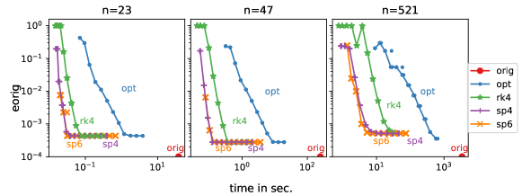
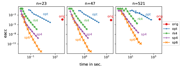
Figure 2: Time–error charts for the conventional and proposed implementations. The top figures are for eorig, and the bottom figures are for eacc. All measurements were performed five times, and log-log-plotted as markers. The lines are the medians for each dz. We placed the results for orig on the x-axis in the top figures to indicate that the eorig value is exactly $0$ by definition.

Time–error charts are shown in Fig. 2. The curves of eorig are saturated around $\mathtt{eorig}\sim 10^{-4}$. This occurs simply because the output format of orig is ’E12.4’, only $4$ digits. Consequently, the new implementations achieve an accuracy that is considered to be sufficient by the developers of the conventional implementation more quickly than orig. Among the new implementations, sp4 and sp6 achieve a sufficient accuracy within the shortest amount of time. The performances of sp4 and sp6 appear to be almost the same in this figure, even though sp6 has a higher order than sp4.

In the figures for eacc, we can see the behaviors of the curves at values below $\mathtt{eorig}<10^{-4}$. The curves for sp6 are the steepest among the new implementations and outperform sp4 at values below $\mathtt{eacc}<10^{-6}$ for n=23 and n=47 and at values below $\mathtt{eacc}<10^{-4}$ for n=521. sp4 and rk4 have almost the same slope, but sp4 is faster than rk4 by one order of magnitude.

Computation time for baseline accuracy

Table 3: Computation time and speed-up rate from orig. We selected the fastest results such that the $\mathtt{eacc}$ value is smaller than that of orig.

data	method	dz	$\mathtt{eacc}$	time in sec.	speed up rate
n=23	orig	$1.000\,000\,000\,000\,000\text{\times}{10}^{-02}$	$4.329\,095\,380\,798\,452\text{\times}{10}^{-04}$	$3.830\,600\,000\,000\,000\text{\times}{10}^{01}$	$1.000\,000\,000\,000\,000\text{\times}{10}^{00}$
	opt	$2.200\,000\,000\,000\,000\text{\times}{10}^{-02}$	$2.524\,585\,847\,350\,836\text{\times}{10}^{-04}$	$1.775\,955\,341\,800\,000\text{\times}{10}^{00}$	$2.156\,923\,606\,039\,293\text{\times}{10}^{01}$
	rk4	$4.700\,000\,000\,000\,000\text{\times}{10}^{-02}$	$2.046\,810\,891\,250\,196\text{\times}{10}^{-04}$	$7.463\,165\,259\,999\,868\text{\times}{10}^{-02}$	$5.132\,674\,765\,398\,493\text{\times}{10}^{02}$
	sp4	$1.500\,000\,000\,000\,000\text{\times}{10}^{-01}$	$3.562\,029\,263\,491\,765\text{\times}{10}^{-05}$	$3.813\,462\,160\,000\,256\text{\times}{10}^{-02}$	$1.004\,494\,036\,988\,096\text{\times}{10}^{03}$
	sp6	$3.300\,000\,000\,000\,000\text{\times}{10}^{-01}$	$6.913\,115\,388\,572\,034\text{\times}{10}^{-05}$	$3.186\,411\,620\,000\,058\text{\times}{10}^{-02}$	$1.202\,167\,345\,849\,665\text{\times}{10}^{03}$
n=47	orig	$1.000\,000\,000\,000\,000\text{\times}{10}^{-02}$	$2.777\,707\,069\,907\,318\text{\times}{10}^{-04}$	$2.516\,040\,000\,000\,000\text{\times}{10}^{02}$	$1.000\,000\,000\,000\,000\text{\times}{10}^{00}$
	opt	$2.200\,000\,000\,000\,000\text{\times}{10}^{-02}$	$2.490\,417\,808\,814\,971\text{\times}{10}^{-04}$	$8.813\,310\,090\,600\,044\text{\times}{10}^{00}$	$2.854\,818\,421\,382\,355\text{\times}{10}^{01}$
	rk4	$4.700\,000\,000\,000\,000\text{\times}{10}^{-02}$	$1.962\,351\,123\,813\,380\text{\times}{10}^{-04}$	$3.579\,840\,540\,000\,305\text{\times}{10}^{-01}$	$7.028\,357\,749\,140\,931\text{\times}{10}^{02}$
	sp4	$2.200\,000\,000\,000\,000\text{\times}{10}^{-01}$	$1.597\,960\,656\,229\,034\text{\times}{10}^{-04}$	$1.232\,810\,935\,999\,851\text{\times}{10}^{-01}$	$2.040\,896\,885\,749\,482\text{\times}{10}^{03}$
	sp6	$3.300\,000\,000\,000\,000\text{\times}{10}^{-01}$	$5.223\,740\,308\,576\,600\text{\times}{10}^{-05}$	$1.361\,412\,525\,999\,867\text{\times}{10}^{-01}$	$1.848\,109\,924\,030\,657\text{\times}{10}^{03}$
n=521	orig	$1.000\,000\,000\,000\,000\text{\times}{10}^{-02}$	$5.151\,892\,346\,217\,075\text{\times}{10}^{-04}$	$3.441\,453\,999\,999\,999\text{\times}{10}^{03}$	$1.000\,000\,000\,000\,000\text{\times}{10}^{00}$
	opt	$1.000\,000\,000\,000\,000\text{\times}{10}^{-02}$	$3.611\,137\,709\,371\,056\text{\times}{10}^{-04}$	$5.955\,675\,777\,463\,991\text{\times}{10}^{02}$	$5.778\,444\,174\,248\,548\text{\times}{10}^{00}$
	rk4	$1.500\,000\,000\,000\,000\text{\times}{10}^{-02}$	$1.470\,262\,355\,964\,512\text{\times}{10}^{-04}$	$2.396\,980\,442\,839\,995\text{\times}{10}^{01}$	$1.435\,745\,548\,229\,208\text{\times}{10}^{02}$
	sp4	$6.800\,000\,000\,000\,000\text{\times}{10}^{-02}$	$9.103\,368\,786\,673\,352\text{\times}{10}^{-05}$	$6.966\,074\,966\,000\,815\text{\times}{10}^{00}$	$4.940\,305\,719\,930\,715\text{\times}{10}^{02}$
	sp6	$1.500\,000\,000\,000\,000\text{\times}{10}^{-01}$	$5.381\,183\,283\,290\,355\text{\times}{10}^{-05}$	$5.183\,526\,088\,799\,772\text{\times}{10}^{00}$	$6.639\,214\,197\,139\,030\text{\times}{10}^{02}$

Table 3 shows the fastest results from Fig. 2, where the $\mathtt{eacc}$ value is less than that of orig with $\mathtt{dz}=0.01$\mathrm{\SIUnitSymbolAngstrom}$$. This table clearly shows that the new implementations outperform orig. opt is more than $20$ times faster than orig then the two improvements described in §3.5 are implemented for n=23 and n=47 and approximately $6$ times faster when one of the two improvements is included for n=521. With the proposed method, rk4, sp4, and sp6 are more than $100$ times faster than orig, and the performance of sp4 shows as improvement of more than $2,000$ fold for n=47.

5 Discussion

Effect of the recursive reflection technique and RHST

It is not fully theoretically understood why the recursive reflection technique and RHST can avoid numerical breakdowns. One reason might be that the physical law bounds some norm of the transfer matrix $R_{i}$ less than $1$ because the reflection wave must have less energy than the input.

The transfer matrix $\hat{A}_{i}$ should have the same property as a physical representation. However, the transfer matrix is an operator which converts the wave at the bottom side to that of the top side and not an operator which converts the input to the output. This is the reason why $\hat{A}_{i}$ can have a norm greater than $1$. If we convert the transfer matrix to separate the input (from the top and bottom) and output (to the bottom and top) at the left and right side of the matrix, the norm of the converted matrix will be less than or equal to $1$.

Need for structure preservation

The conventional method uses the second-order Magnus method  [29], which is a Lie-group method that can maintain a Lie-group structure if the equation has such a structure. The ODE solvers that we used for our proposed method in the test cannot maintain such a structure. Thus, this might be a regression from the conventional method.

As far as we know, the equation has no interesting Lie-group structure because the potential $v$ has an artificial imaginary component that represents the absorption effect. Therefore, the structure is $\mathrm{GL}(2n)$, which is the group of non-singular matrices.

If the geometry is important, higher-order Magnus-based methods for second-order non-autonomous ODEs are available [35].

Application of the proposed method to other simulations

Our goal in this study was to improve upon conventional methods and implementations currently in use. At this stage, the proposed method is specific to RHEED/TRHEPD, but may possibly be applicable to other many-beam reflective diffraction simulations that have severe ill-conditionedness.

Note that if the problem is well-conditioned, i.e., if the matrix product $\hat{A}_{0}\hat{A}_{1}\cdots$ has a small condition number, we can use simple linear solvers to solve BVP. The generalized minimum residual method (GMRES) will be the best method in this case, because the method does not require computing the explicit components of the matrix product.

6 Conclusion

In this article, we proposed a new method for faster RHEED/TRHEPD simulations of the conventional ones. Our strategy is standard, reformulates BVP as an initial-value matrix ODE, and applies high-order ODE solvers such as fourth-order Runge-Kutta and splitting methods, except for the generalization of the recursive reflection technique to the RHST. As a result, our proposed method reduces the number of computations and increases the computation efficiency while maintaining the same accuracy as that of the conventional method. Moreover, we also proposed a high-performance implementation of the algorithm to utilize the multi-thread parallelism and cache memory performance of recent CPUs.

In our performance evaluation based on three test problems, our new implementations of the proposed algorithm outperform the conventional method by orders of magnitude, up to $2,000$ fold. This huge leap in speed from the conventional method not only reduces the cost of simulations, but also widens the ability of reverse analysis, for example, by allowing the number of parameters to be increased for optimization or enabling reverse analysis to be performed immediately after measurements without supercomputers.

Most of the computation of the algorithm presented herein consists of matrix multiplications, which are well-suited for accelerators such as graphic processing units (GPUs), except for the RHST step. As a future work, it may be beneficial to develop a better method for the RHST that emplys uniform computational patterns with lower or similar computational costs while maintaining the ability to avoid numerical breakdowns. The accuracy of the simulation with lower-precision (single or half) could also be evaluated in the future to utilize the processing power of these accelerators.

Declaration of competing interest

The authors have no conflicts of interest to declare that are relevant to the content of this article.

Data statement

All the source codes and obtained data are available at github.com/shuheikudo/trhepd-opt.