A polynomial-time iterative algorithm for random graph matching with non-vanishing correlation

Abstract

We propose an efficient algorithm for matching two correlated Erdős–Rényi graphs with $n$ vertices whose edges are correlated through a latent vertex correspondence. When the edge density $q=n^{-\alpha+o(1)}$ for a constant $\alpha\in[0,1)$, we show that our algorithm has polynomial running time and succeeds to recover the latent matching as long as the edge correlation is non-vanishing. This is closely related to our previous work on a polynomial-time algorithm that matches two Gaussian Wigner matrices with non-vanishing correlation, and provides the first polynomial-time random graph matching algorithm (regardless of the regime of $q$) when the edge correlation is below the square root of the Otter’s constant (which is $\approx 0.338$).

1 Introduction

In this paper, we study the algorithmic perspective for recovering the latent matching between two correlated Erdős–Rényi graphs. To be mathematically precise, we first need to choose a model for a pair of correlated Erdős–Rényi graphs, and a natural choice is that the two graphs are independently sub-sampled from a common Erdős–Rényi graph, as describe more precisely next. For two vertex sets $V$ and $\mathsf{V}$ with cardinality $n$, let $E_{0}$ be the set of unordered pairs $(u,v)$ with $u,v\in V,u\neq v$ and define $\mathsf{E}_{0}$ similarly with respect to $\mathsf{V}$. For some model parameters $p,s\in(0,1)$, we generate a pair of correlated random graphs $G=(V,E)$ and $\mathsf{G}=(\mathsf{V},\mathsf{E})$ with the following procedure: sample a uniform bijection $\pi:V\to\mathsf{V}$, independent Bernoulli variables $I_{(u,v)}$ with parameter $p$ for $(u,v)\in E_{0}$ as well as independent Bernoulli variables $J_{(u,v)},\mathsf{J}_{(\mathsf{u},\mathsf{v})}$ with parameter $s$ for $(u,v)\in E_{0}$ and $(\mathsf{u},\mathsf{v})\in\mathsf{E}_{0}$. Let

$$G_{(u,v)}=I_{(u,v)}J_{(u,v)},\forall(u,v)\in E_{0}\,,\quad\mathsf{G}_{(\mathsf{u},\mathsf{v})}=I_{\left(\pi^{-1}(\mathsf{u}),\pi^{-1}(\mathsf{v})\right)}\mathsf{J}_{(\mathsf{u},\mathsf{v})},\forall(\mathsf{u},\mathsf{v})\in\mathsf{E}_{0}\,,$$ (1.1)

and let $E=\{e\in E_{0}:G_{e}=1\},\mathsf{E}=\{\mathsf{e}\in\mathsf{E}_{0}:\mathsf{G}_{\mathsf{e}}=1\}$. It is obvious that marginally $G$ is an Erdős–Rényi graph with edge density $q=ps$ and so is $\mathsf{G}$. In addition, the edge correlation $\rho$ is given by $\rho=s(1-p)/(1-ps)$.

An important question is to recover the latent matching $\pi$ from the observation of $(G,\mathsf{G})$. More precisely, we wish to find an estimator $\hat{\pi}$ which is measurable with respect to $(G,\mathsf{G})$ such that $\hat{\pi}=\pi$. Our main contribution is an efficient matching algorithm as incorporated in the theorem below.

Theorem 1.1.

Suppose that $q=n^{-\alpha+o(1)}\leq 1/2$ for some constant $\alpha\in[0,1)$ and that $\rho\in(0,1]$ is a constant. Then there exist a constant $C=C(\alpha,\rho)$ and an algorithm (see Algorithm 2.6 below) with time-complexity $O(n^{C})$ that recovers the latent matching with probability $1-o(1)$. That is, this polynomial-time algorithm takes $(G,\mathsf{G})$ as the input and outputs an estimator $\hat{\pi}$ such that $\hat{\pi}=\pi$ with probability tending to 1 as $n\to\infty$.

1.1 Backgrounds and related works

Motivated by questions from applied fields such as social network analysis [36, 37], computer vision [8, 4], computational biology [44, 45] and natural language processing [27], the random graph matching problem has been extensively studied recently. By the collective efforts as in [10, 9, 28, 49, 48, 25, 13, 14], it is fair to say that we have fairly complete understanding on the information thresholds for the problem of correlation detection and vertex matching. In contrast, the understanding on the computational aspect is far from being complete, and in what follows we briefly review the progress on this front.

A huge amount of efforts have been devoted to developing efficient algorithms for graph matching [38, 50, 31, 30, 22, 43, 1, 17, 19, 20, 5, 11, 12, 35, 24, 32, 34, 26, 33]. Previous to this work, arguably the best result is the recent work [33] (see also [26] for a remarkable result on partial recovery of similar flavor when the average degree is $O(1)$), where the authors substantially improved a groundbreaking work [32] and obtained a polynomial time algorithm which succeeds as long as the correlation is above the square root of the Otter’s constant (the Otter’s constant is around ${0.338}$). In terms of methods, the present work seems drastically different from these existing works; instead, this work is closely related to our previous work [16] on a polynomial-time iterative algorithm that matches two correlated Gaussian Wigner matrices. One is encouraged to see [33, Section 1.1] and [16, Section 1.1] for a more elaborated review on previous algorithms. In addition, one is encouraged to see [16, Section 1.2] for discussions on novel features of this iterative algorithm, especially in comparison with the message-passing algorithm [26, 39] and a recent greedy algorithm for aligning two independent graphs [15].

1.2 Our contributions

While the present work can be viewed as an extension of [16], we do feel that we have conquered substantial obstacles and have made substantial contributions to this topic, as we describe below.

• While in [33] (see also [26]) polynomial-time matching algorithms were obtained when the correlation is above the threshold from the Otter’s constant, our work establishes a polynomial-time algorithm as long as the average degree grows polynomially and the correlation is non-vanishing. In addition, the power in the running time only tends to $\infty$ as the correlation tends to $0$ (for each fixed $\alpha<1$), and we are under the feeling that this is the best possible.

• From a conceptual point of view, our work demonstrates the robustness of the iterative matching algorithm proposed in [16]. This type of “algorithmic universality” is closely related to the universality phenomenon in random matrix theory, which roughly speaking postulates that the particular distribution for entries of random matrices is often irrelevant for spectral properties under investigation. Our work also encourages future study on even more ambitious perspectives for robustness, for instance algorithms that are robust with assumptions on underlying random graph models. This is of major interest since realistic networks are usually captured better by more structured graph models, such as the random geometric graph model [46], the random growing graph model [40] and the stochastic block model [41].

• In terms of techniques, our work employs a method which argues that Gaussian approximation is valid typically. There are a couple of major challenges : (1) Gaussian approximation is valid only in a rather weak sense that the Radon-Nikodym derivative is not too large; (2) we can not simply ignore the atypical cases when Gaussian approximation is invalid since we have to analyze the conditional behavior given all the information the algorithm has exploited so far. The latter raises a major obstacle in our proof for theoretical guarantee; see Section 3.1 for more detailed discussions on how this obstacle is addressed.

In addition, it is natural to suspect that our work brings us one step closer to understanding computational phase transitions for random graph matching problems as well as understanding algorithmic perspectives for other matching problems (see, e.g., [6]). We refer an interested reader to [16, Section 1.3] and omit further discussions here.

1.3 Notations

We record in this subsection some notation conventions.

Denote the identity matrix by $\mathrm{I}$ and the zero matrix by $\mathrm{O}$. For a $d*m$ matrix $\mathrm{A}$, we use $\mathrm{A}^{*}$ to denote its transpose, and let $\|\mathrm{A}\|_{\mathrm{HS}}$ denote the Hilbert-Schmidt norm of $\mathrm{A}$. For $1\leq s\leq\infty$, define the $s$-norm of $\mathrm{A}$ by $\|\mathrm{A}\|_{s}=\sup\{\|\mathrm{A}x\|_{t}:\|x\|_{t}=1\}$, where $\frac{1}{s}+\frac{1}{t}=1$. We further denote the operator norm of $\mathrm{A}$ by $\|\mathrm{A}\|_{\mathrm{op}}=\|\mathrm{A}\|_{2}$. If $m=d$, denote $\mathrm{det(A)}$ and $\mathrm{tr(A)}$ the determinant and the trace of $\mathrm{A}$, respectively. For $d$-dimensional vectors $x,y$ and a $d*d$ symmetric matrix $\Sigma$, let $\langle x,y\rangle_{\Sigma}=x\Sigma y^{*}$ be the “inner product” of $x,y$ with respect to $\Sigma$, and we further denote $\|x\|_{\Sigma}^{2}=x\Sigma x^{*}$. For two vectors $\gamma,\mu\in\mathbb{R}^{d}$, we say $\gamma\geq\mu$ (or equivalently $\mu\leq\gamma$) if their entries satisfy $\gamma(i)\geq\mu(i)$ for all $1\leq i\leq d$. The indicator function of a set $A$ is denoted by $\mathbf{I}_{A}$.

Without further specification, all asymptotics are taken with respect to $n\to\infty$. We also use standard asymptotic notations: for two sequences $\{a_{n}\}$ and $\{b_{n}\}$, we write $a_{n}=O(b_{n})$ or $a_{n}\lesssim b_{n}$, if $|a_{n}|\leq C|b_{n}|$ for some absolute constant $C$ and all $n$. We write $a_{n}=\Omega(b_{n})$ or $a_{n}\gtrsim b_{n}$, if $b_{n}=O(a_{n})$; we write $a_{n}=\Theta(b_{n})$ or $a_{n}\asymp b_{n}$, if $a_{n}=O(b_{n})$ and $a_{n}=\Omega(b_{n})$; we write $a_{n}=o(b_{n})$ or $b_{n}=\omega(a_{n})$, if $\frac{a_{n}}{b_{n}}\to 0$ as $n\to\infty$. We write $a_{n}\sim b_{n}$ if $\frac{a_{n}}{b_{n}}\to 1$.

We denote by $\mathrm{Ber}(p)$ the Bernoulli distribution with parameter $p$, denote by $\mathrm{Bin}(n,p)$ the Binomial distribution with $n$ trials and success probability $p$, denote by $\mathcal{N}(\mu,\sigma^{2})$ the normal distribution with mean $\mu$ and variance $\sigma^{2}$, and denote by $\mathcal{N}(\mu,\Sigma)$ the multi-variate normal distribution with mean $\mu$ and covariance matrix $\Sigma$. We say $(X,Y)$ is a pair of correlated binomial random variables, denoted as $\mathrm{CorBin}(N,M,p;m,\rho)$ for $m\leq\min\{N,M\}$ and $\rho\in[0,1]$, if $(X,Y)\sim(\sum_{k=1}^{N}b_{k},\sum_{k=1}^{M}b^{\prime}_{k})$ with $b_{k},b^{\prime}_{l}\sim\mathrm{Ber}(p)$ such that $\{b_{k},b^{\prime}_{k}\}$ are independent with $\{b_{1},\ldots,b_{N},b^{\prime}_{1},\ldots,b^{\prime}_{M}\}\setminus\{b_{k},b^{\prime}_{k}\}$ and the covariance between $b_{k}$ and $b^{\prime}_{k}$ is $\rho$ when $k\leq m$, and that $b_{k}$ is independent with $\{b_{1},\ldots,b_{N},b^{\prime}_{1},\ldots,b^{\prime}_{M}\}\setminus\{b_{k}\}$ and $b^{\prime}_{l}$ is independent with $\{b_{1},\ldots,b_{N},b^{\prime}_{1},\ldots,b^{\prime}_{M}\}\setminus\{b^{\prime}_{l}\}$ when $k,l>m$. We say $X$ is a sub-Gaussian variable, if there exists a positive constant $C$ such that $\mathbb{P}[|X|\geq t]\leq 2e^{-{t^{2}}/{C^{2}}}$, and we use $\|X\|_{\psi_{2}}=\inf\{C>0:\mathbb{E}[\exp\{\frac{X^{2}}{C^{2}}\}]\leq 2\}$ to denote its sub-Gaussian norm.

Acknowledgment. We thank Zongming Ma, Yihong Wu, Jiaming Xu and Fan Yang for stimulating discussions on random graph matching problems. J. Ding is partially supported by NSFC Key Program Project No. 12231002.

2 An iterative matching algorithm

We first describe the underlying heuristics of our algorithm (the reader is strongly encouraged to consult [16, Section 2] for a description on the iterative matching algorithm for correlated Gaussian Wigner matrices). Since we expect that Wigner matrices and Erdős–Rényi graphs (with sufficient edge density) should belong to the same algorithmic universality class, it is natural to try to extend the algorithm proposed in [16] to the case for correlated random graphs. As in [16], our wish is to iteratively construct a sequence of paired sets $(\Gamma^{(t)}_{k},\Pi^{(t)}_{k})_{1\leq k\leq K_{t}}$ for $t\geq 0$ (with $\Gamma^{(t)}_{k}\subset V$ and $\Pi^{(t)}_{k}\subset\mathsf{V}$), where each $(\Gamma^{(t)}_{k},\Pi^{(t)}_{k})$ contains more true pairs of the form $(v,\pi(v))$ than the case when the two sets are sampled uniformly and independently.

For initialization in [16], we obtain $K_{0}$ true pairs via brute-force search, and provided with $K_{0}$ true pairs we then for each such pair define $(\Gamma^{(0)}_{k},\Pi^{(0)}_{k})$ to be the collections of their neighbors such that the corresponding edge weights exceed a certain threshold. In this work, however, due to the sparsity of Erdős–Rényi graphs (when $\alpha>0$) we cannot produce an efficient initialization by simply looking at the 1-neighborhoods of some true pairs. In order to address this, we instead look at their $\chi$-neighborhoods with carefully chosen $\chi$ (see the definition of $(\Gamma^{(0)}_{k},\Pi^{(0)}_{k})$ in (2.5) below). This would require a significantly more complicated analysis since this initialization will have influence on iterations later. The idea to address this is to argue that in the initialization we have only used information on a small fraction of the edges; this is why $\chi$ will be chosen carefully.

Provided with the initialization, the iteration of the algorithm is similar to that in [16] (although we will introduce some modifications in order to facilitate our analysis later). Since each pair $(\Gamma^{(t)}_{k},\Pi^{(t)}_{k})$ carries some signal, we then hope to construct more paired sets at time $t+1$ by considering various linear combinations of vertex degrees restricted to each $\Gamma^{(t)}_{k}$ (or to $\Pi^{(t)}_{k}$). As a key novelty of this iterative algorithm, as in [16] we will use the increase on the number of paired sets to compensate the decrease on the signal carried in each pair. As we hope, once the iteration progresses to time $t=t^{*}$ for some well chosen $t^{*}$ (see (2.23) below) we would have accumulated enough total signal so that we can just complete the matching directly in the next step, as described in Section 2.4.

However, controlling the correlation among different iterative steps is a much more sophisticated job in this setting. In [16] we used Gaussian projection to remove the influence of conditioning on information obtained in previous steps. This is indeed a powerful technique but it crucially relies on the property of Gaussian process. Although there are examples that the universality of iterative algorithms have been established (see, e.g., [2, 7, 21] for development on this front for approximate-message-passing), we are not sure how their techniques can help solving our problem since dealing with a pair of correlated matrices seems of substantial and novel challenge. Instead we try to compare the Bernoulli process we obtained in the iterative algorithm with the corresponding Gaussian process when we replace $\{G_{u,v},\mathsf{G}_{\mathsf{u,v}}\}$ by a Gaussian process with the same mean and covariance structure. In order to facilitate such comparison, we also apply a Gaussian smoothing to our Bernoulli process in our algorithm below (see (2.22) where we introduce external Gaussian noise for smoothing purpose). However, since we need to analyze the conditional behavior of two processes, we need to compare their densities; this is much more demanding than controlling e.g. the transportation distance between two processes, and actually the density ratio of these two processes are fairly large. In order to address this, on the one hand we will show that mostly (i.e., if we ignore a vanishing fraction of vertices, which is a highly non-trivial step as we will elaborate in Section 3.1) the density ratio is then under control while still being fairly large, and on the other hand we show that in the Gaussian setting really bad event occurs with tiny probability (and thus still with small probability even after multiplying by the fairly large density ratio). We refer to Sections 3.4 and 3.5 for more detailed discussions on this point.

Finally, due to aforementioned complications we are only able to show that our iterative algorithm constructs an almost exact matching. To obtain an exact matching, we will employ the method of seeded graph matching, as developed in previous works [1, 35, 33].

In the rest of this section, we will describe in detail our iterative algorithm, which consists of a few steps including preprocessing (see Section 2.1), initialization (see Section 2.2), iteration (see Section 2.3), finishing (see Section 2.4) and seeded graph matching (see Section 2.5). We formally present our algorithm in Section 2.6. In Section 2.7 we analyze the time complexity of the algorithm.

2.1 Preprocessing

Similar to [16], we make appropriate preprocessing on random graphs such that we only need to consider graphs with directed edges. We first make a technical assumption that we only need to consider the case when $\rho$ is a sufficiently small constant, which can be easily achieved by keeping each edge independently with a sufficiently small constant probability.

Now, we define $\overrightarrow{G}$ from $G$. For any $u\neq v\in V$, we do the following:

• if $(u,v)\in E(G)$, then independently among all such $(u,v)$:

  $$\mbox{with probability }\frac{1}{2}-\frac{q}{4},\mbox{ set }\overrightarrow{(u,v)}\in\overrightarrow{G},\overrightarrow{(v,u)}\not\in\overrightarrow{G}\,,$$

  $$\mbox{with probability }\frac{1}{2}-\frac{q}{4},\mbox{ set }\overrightarrow{(u,v)}\not\in\overrightarrow{G},\overrightarrow{(v,u)}\in\overrightarrow{G}\,,$$

  $$\mbox{with probability }\frac{q}{4},\mbox{ set }\overrightarrow{(u,v)}\in\overrightarrow{G},\overrightarrow{(v,u)}\in\overrightarrow{G}\,,$$

  $$\mbox{with probability }\frac{q}{4},\mbox{ set }\overrightarrow{(u,v)}\not\in\overrightarrow{G},\overrightarrow{(v,u)}\not\in\overrightarrow{G}\,;$$

• if $(u,v)\not\in E(G)$, then set $\overrightarrow{(u,v)}\not\in\overrightarrow{G},\overrightarrow{(v,u)}\not\in\overrightarrow{G}$.

We define $\overrightarrow{\mathsf{G}}$ from $\mathsf{G}$ in the same manner such that $\overrightarrow{G}$ and $\overrightarrow{\mathsf{G}}$ are conditionally independent given $(G,\mathsf{G})$. We continue to use the convention that $\overrightarrow{G}_{u,v}=\mathbf{I}_{\{\overrightarrow{(u,v)}\in\overrightarrow{G}\}}$. It is then straightforward to verify that $\{\overrightarrow{G}_{u,v}:u\neq v\}$ and $\{\mathsf{\overrightarrow{\mathsf{G}}_{u,v}:u\neq v}\}$ are two families of i.i.d. Bernoulli random variables with parameter $\frac{q}{2}$. In addition, we have

$$\mathbb{E}[\overrightarrow{G}_{u,v}{\overrightarrow{\mathsf{G}}_{\pi(u),\pi(v)}}]=\mathbb{E}[\overrightarrow{G}_{u,v}{\overrightarrow{\mathsf{G}}_{\pi(v),\pi(u)}}]=\frac{q(q+\rho(1-q))}{4}\,.$$

Thus, $\overrightarrow{G},\overrightarrow{\mathsf{G}}$ are edge-correlated directed graphs, denoted as $\overrightarrow{\mathcal{G}}(n,\hat{q},\hat{\rho})$, such that $\hat{q}=\frac{q}{2}$ and $\hat{\rho}=\frac{1-q}{2-q}\rho$. Also note that $\hat{q}\geq n^{-\alpha+o(1)}$ and $\hat{\rho}\in[\frac{\rho}{3},\frac{\rho}{2})$ since $q\leq 1/2$. From now on we will work on the directed graph $(\overrightarrow{G},\overrightarrow{\mathsf{G}})$.

2.2 Initialization

Let $\kappa=\kappa(\hat{\rho})$ be a sufficiently large constant depending on $\hat{\rho}$ whose exact value will be decided later in (2.24). Set $K_{0}=\kappa$. We then arbitrarily choose a sequence $A=(u_{1},u_{2},\ldots,u_{K_{0}})$ where $u_{i}$’s are distinct vertices in $V$, and we list all the sequences of length $K_{0}$ with distinct elements in $\mathsf{V}$ as $\mathsf{A}_{1},\mathsf{A}_{2},\ldots,\mathsf{A}_{\mathtt{M}}$ where $\mathtt{M}=\mathtt{M}(n,\hat{\rho},\hat{q})=\prod_{i=0}^{K_{0}-1}(n-i)$. As in [16], for each $1\leq\mathtt{m}\leq\mathtt{M}$, we will run a procedure of initialization and iteration and clearly for one of them (although a priori we do not know which one it is) we are running the algorithm as if we have $K_{0}$ true pairs as seeds. For convenience, when describing the initialization and the iteration we will drop $\mathtt{m}$ from notations, but we emphasize that this procedure will be applied to each $\mathsf{A}_{\mathtt{m}}$. Having this clarified, we take a fixed $\mathtt{m}$ and denote $\mathsf{A}_{\mathtt{m}}=\{\mathsf{u}_{1},\mathsf{u}_{2},\ldots,\mathsf{u}_{K_{0}}\}$. In what follows, we abuse the notation and write $V\setminus A$ when regarding $A$ as a set (similarly for $\mathsf{A}_{\mathtt{m}}$).

We next describe our initialization procedure. As discussed earlier, to the contrary of the case for Wigner matrices, we have to investigate the neighborhood around a seed up to a certain depth in order to get information for a large number of vertices. To this end, we choose an integer $\chi\leq\frac{1}{1-\alpha}$ as the depth such that

$$(n\hat{q})^{\chi}=o(ne^{-(\log\log n)^{100}})\mbox{ and }(n\hat{q})^{\chi+1}=\Omega(ne^{-(\log\log n)^{100}})$$ (2.1)

(this is possible since $\alpha<1$). We choose such $\chi$ since on the one hand we wish to see a large number of vertices near the seed and on the other hand we want to reveal only a vanishing fraction of the edges. Now for $1\leq k\leq K_{0}$, define

$$\aleph^{(0)}_{k}=\{u_{k}\},\Upsilon^{(0)}_{k}=\{\mathsf{u}_{k}\}\,,\mbox{ and }\vartheta_{0}=\varsigma_{0}=1/n\,.$$ (2.2)

Then for $1\leq a\leq\chi$, we iteratively define

$$\aleph^{(a)}_{k}=\Big{\{}v\in V\setminus\big{(}\cup_{1\leq k\leq K_{0},0\leq j\leq a-1}\aleph^{(j)}_{k}\big{)}:\overrightarrow{G}_{v,u}=1\mbox{ for some }u\in\aleph^{(a-1)}_{k}\Big{\}}\,,$$ (2.3)

$$\Upsilon^{(a)}_{k}=\Big{\{}\mathsf{v}\in\mathsf{V}\setminus\big{(}\cup_{1\leq k\leq K_{0},0\leq j\leq a-1}\Upsilon^{(j)}_{k}\big{)}:\overrightarrow{\mathsf{G}}_{\mathsf{v},\mathsf{u}}=1\mbox{ for some }\mathsf{u}\in\Upsilon^{(a-1)}_{k}\Big{\}}\,.$$

Also, for $1\leq a\leq\chi$ we iteratively define

$$\vartheta_{a}=\mathbb{P}(X\geq 1)\mbox{ where }X\sim\mathrm{Bin}(\vartheta_{a-1}n,\hat{q})\,,$$ (2.4)

$$\varsigma_{a}=\mathbb{P}(X\geq 1,Y\geq 1)\mbox{ where }(X,Y)\sim\mathrm{CorBin}(\vartheta_{a-1}n,\vartheta_{a-1}n,\hat{q};\varsigma_{a-1}n,\hat{\rho})\,.$$

Let $\mathtt{d}_{\chi}=\mathtt{d}_{\chi}(n,\hat{q})$ be the minimal integer such that $\mathbb{P}(\mathrm{Bin}(n\vartheta_{\chi},\hat{q})\geq\mathtt{d}_{\chi})<\frac{1}{2}$, and set

$$\Gamma^{(0)}_{k}=\aleph^{(\chi+1)}_{k}=\Big{\{}v\in V\setminus\big{(}\cup_{1\leq k\leq K_{0},0\leq j\leq\chi}\aleph^{(j)}_{k}\big{)}:\sum_{u\in\aleph^{(\chi)}_{k}}\overrightarrow{G}_{v,u}\geq\mathtt{d}_{\chi}\Big{\}}\,,$$ (2.5)

$$\Pi^{(0)}_{k}=\Upsilon^{(\chi+1)}_{k}=\Big{\{}\mathsf{v}\in\mathsf{V}\setminus\big{(}\cup_{1\leq k\leq K_{0},0\leq j\leq\chi}\Upsilon^{(j)}_{k}\big{)}:\sum_{\mathsf{u}\in\Upsilon^{(\chi)}_{k}}\overrightarrow{\mathsf{G}}_{\mathsf{v},\mathsf{u}}\geq\mathtt{d}_{\chi}\Big{\}}\,.$$

And we further define

$$\vartheta=\vartheta_{\chi+1}=\mathbb{P}(X\geq\mathtt{d}_{\chi})\mbox{ where }X\sim\mathrm{Bin}(\vartheta_{\chi}n,\hat{q})\,,$$ (2.6)

$$\varsigma=\varsigma_{\chi+1}=\mathbb{P}(X,Y\geq\mathtt{d}_{\chi})\mbox{ where }X,Y\sim\mathrm{CorBin}(\vartheta_{\chi}n,\vartheta_{\chi}n,\hat{q};\varsigma_{\chi}n,\hat{\rho}))\,.$$

In addition, we define $\Phi^{(0)},\Psi^{(0)}$ to be $K_{0}\times K_{0}$ matrices by

$$\Phi^{(0)}=\mathrm{I}\mbox{ and }\Psi^{(0)}=\frac{\varsigma-\vartheta^{2}}{2(\vartheta-\vartheta^{2})}\mathrm{I}\,,$$ (2.7)

and in the iterative steps we will also construct $\Phi^{(t)}$ and $\Psi^{(t)}$ for $t\geq 1$. We conclude this subsection with some bounds on $(\vartheta_{k},\varsigma_{k})$.

Lemma 2.1.

$\vartheta_{k},\varsigma_{k}=\Theta(n^{-1}(n\hat{q})^{k})$ for $0\leq k\leq\chi$ and $\vartheta_{\chi+1},\varsigma_{\chi+1}=\Omega(e^{-(\log\log n)^{100}})$. Also, we have $\varsigma_{k}-\vartheta_{k}^{2}=\Theta(\vartheta_{k})$ for $0\leq k\leq\chi+1$. In addition, we have either $\vartheta_{\chi+1}=\Theta(1)$ or $\vartheta_{\chi}\leq n^{-\alpha+o(1)}$.

Proof.

We prove the first claim by induction. The claim is trivial for $k=0$. Now suppose the claim holds up to some $k\leq\chi-1$. Using (2.4) and Poisson approximation (note that when $k\leq\chi-1$ we have $n\hat{q}\vartheta_{k}=\Theta(n^{-1}(n\hat{q})^{k+1})=o(1)$)

$$\vartheta_{k+1}=\Theta((\vartheta_{k}n\hat{q})=\Theta(n^{-1}(n\hat{q})^{k+1})\mbox{ and }\vartheta_{k+1}\geq\varsigma_{k+1}\geq\Theta(\hat{\rho}\varsigma_{k}n\hat{q})=\Theta(\vartheta_{k+1})\,,$$

which verifies the claim for $k+1$ and thus verifies the first claim (for $0\leq k\leq\chi$). If $\vartheta_{\chi}n\hat{q}=\Theta((n\hat{q})^{\chi+1})\ll 1$, we have $\mathtt{d}_{\chi}=1$ and thus $\vartheta_{\chi+1},\varsigma_{\chi+1}=\Theta((n\hat{q})^{\chi+1})=\Omega(e^{-(\log\log n)^{100}})$; if $\vartheta_{\chi}n\hat{q}=\Omega(1)$, we have $\varsigma_{\chi}n\hat{q}=\Omega(1)$ and thus by the choice of $\mathtt{d}_{\chi}$ we have $\vartheta_{\chi+1},\varsigma_{\chi+1}=\Theta(1)$ and $\varsigma_{\chi+1}-\vartheta_{\chi+1}^{2}=\Theta(1)$ using Poisson approximation. Thus, we have $\varsigma_{k}-\vartheta_{k}^{2}=\Theta(\vartheta_{k})$ for $k=\chi+1$ (note that the case for $1\leq k\leq\chi+1$ can be checked in a straightforward manner). In addition, if $\vartheta_{\chi}=n^{-\alpha+\epsilon+o(1)}$ for some arbitrarily small but fixed $\epsilon>0$, then $n\hat{q}\vartheta_{\chi}\gg 1$ and thus $\vartheta_{\chi+1}=\Theta(1)$. This completes the proof of the lemma. ∎

2.3 Iteration

For a pair of standard bivariate normal variables $(X,Y)$ with correlation $u$, we define $\phi:[-1,1]\mapsto[0,1]$ by (below the number 10 is somewhat arbitrarily chosen)

$$\phi(u)=\mathbb{P}(|X|\geq 10,|Y|\geq 10)\,.$$ (2.8)

In addition, we define $\iota_{\mathrm{ub}}=\sup_{x\in(0,1]}\big{\{}\frac{\phi(x)-\phi(0)}{x^{2}}\big{\}}$ and $\iota_{\mathrm{lb}}=\inf_{x\in(0,1]}\big{\{}\frac{\phi(x)-\phi(0)}{x^{2}}\big{\}}$. From the definition we know $\phi$ is strictly increasing and by [16, Claims 2.6 and 2.8] we have $\phi^{\prime}(0)=0,\phi^{\prime\prime}(0)>0$, and thus both $\iota_{\mathrm{ub}}$ and $\iota_{\mathrm{lb}}$ are positive and finite. Also we write $\mathfrak{a}=\phi(1)=\mathbb{P}[|X|\geq 10]$. We reiterate that in this subsection we are describing the iteration for a fixed $1\leq\mathtt{m}\leq\mathtt{M}$ and eventually this iterative procedure will be applied to each $\mathtt{m}$. Define

$$\varepsilon_{0}=\frac{\varsigma-\vartheta^{2}}{2(\vartheta-\vartheta^{2})}\mbox{ and }K_{t+1}=\frac{1}{\varkappa}K_{t}^{2}\mbox{ for }t\geq 0\,,$$ (2.9)

where we set $\varkappa=\varkappa(\hat{\rho})=\frac{10^{30}\iota_{\mathrm{ub}}^{2}\hat{\rho}^{-20}}{\iota_{\mathrm{lb}}^{2}(\mathfrak{a}-\mathfrak{a}^{2})^{2}}$. Define

$$D^{(0)}_{v}(k) =\frac{1}{\sqrt{(\vartheta-\vartheta^{2})n\hat{q}(1-\hat{q})}}\sum_{u\in V}(\mathbf{I}_{u\in\Gamma^{(0)}_{k}}-\vartheta)(\overrightarrow{G}_{v,u}-\hat{q})\,,$$ (2.10)

$$\mathsf{D}^{(0)}_{\mathsf{v}}(k) =\frac{1}{\sqrt{(\vartheta-\vartheta^{2})n\hat{q}(1-\hat{q})}}\sum_{\mathsf{u}\in\mathsf{V}}(\mathbf{I}_{\mathsf{u}\in\Pi^{(0)}_{k}}-\vartheta)(\overrightarrow{\mathsf{G}}_{\mathsf{v,u}}-\hat{q})\,.$$

For $t\geq 1$, we now suppose that $(\Gamma^{(s)}_{k},\Pi^{(s)}_{k})_{1\leq k\leq K_{s}}$ has been constructed for $s\leq t$ (which will be implemented inductively via (2.22)). For $v\in V$ and $\mathsf{v}\in\mathsf{V}$, define $D^{(t)}_{v},\mathsf{D}^{(t)}_{\mathsf{v}}\in\mathbb{R}^{K_{t}}$ to be the “normalized degrees” of $v$ in $\Gamma^{(t)}_{k}$ and of $\mathsf{v}$ in $\Pi^{(t)}_{k}$ as follows:

$$D^{(t)}_{v}(k) =\frac{1}{\sqrt{(\mathfrak{a}-\mathfrak{a}^{2})n\hat{q}(1-\hat{q})}}\sum_{u\in V}(\mathbf{I}_{u\in\Gamma^{(t)}_{k}}-\mathfrak{a})(\overrightarrow{G}_{v,u}-\hat{q})\,,$$ (2.11)

$$\mathsf{D}^{(t)}_{\mathsf{v}}(k) =\frac{1}{\sqrt{(\mathfrak{a}-\mathfrak{a}^{2})n\hat{q}(1-\hat{q})}}\sum_{\mathsf{u}\in\mathsf{V}}(\mathbf{I}_{\mathsf{u}\in\Pi^{(t)}_{k}}-\mathfrak{a})(\overrightarrow{\mathsf{G}}_{\mathsf{v,u}}-\hat{q})\,.$$

We note that there is a difference between the definition (2.10) for $t=0$ and the definition (2.11) for $t\geq 1$; this is because $\Gamma^{(0)}_{k}$ and $\Pi^{(0)}_{k}$ may only contain a vanishing fraction of vertices. Recall (2.7). In order to further describe our iterative step we will also need an important property, as in [16, Lemma 2.1], on eigenvalues for $\Phi^{(t)}$ and $\Psi^{(t)}$ (see (2.15)).

Lemma 2.2.

Let $(\Phi^{(t)},\Psi^{(t)})$ be initialized as in (2.7) and inductively defined as in (2.15), also let $\varepsilon_{t}$ be initialized in (2.9) and iteratively defined in (2.20). Then, $\Phi^{(t)}$ has $\frac{3}{4}K_{t}$ eigenvalues between $0.9$ and $1.1$, and $\Psi^{(t)}$ has $\frac{3}{4}K_{t}$ eigenvalues between $0.9\varepsilon_{t}$ and $1.1\varepsilon_{t}$.

Assuming Lemma 2.2, we can then write $\Phi^{(t)}$ and $\Psi^{(t)}$ as their spectral decompositions:

$$\Phi^{(t)}=\sum^{K_{t}}_{i=1}\lambda^{(t)}_{i}\left({\nu^{(t)}_{i}}\right)^{*}\left(\nu^{(t)}_{i}\right)\mbox{ and }\Psi^{(t)}=\sum_{i=1}^{K_{t}}\mu^{(t)}_{i}\left({\xi^{(t)}_{i}}\right)^{*}\left(\xi^{(t)}_{i}\right)$$ (2.12)

where

$$\lambda^{(t)}_{i}\in(0.9,1.1),\mu^{(t)}_{i}\in(0.9\varepsilon_{t},1.1\varepsilon_{t})\mbox{ for }1\leq i\leq\frac{3K_{t}}{4}$$ (2.13)

and $\nu_{i},\xi_{i}$ are the unit eigenvectors with respect to $\lambda_{i},\mu_{i}$ respectively. We sample $\beta^{(t)}_{k}(j)$ as i.i.d. uniform variables on $\{-1,1\}$. By [16, Proposition 2.4], these $\beta^{(t)}_{k}(j)$’s satisfy [16, (2.21)–(2.24)] with probability at least 0.5. As in [16], we will keep resampling until these requirements are satisfied. Define

$$\sigma_{k}^{(t)}=\sqrt{\frac{12}{K_{t}}}\sum_{j=1}^{\frac{1}{12}K_{t}}\beta^{(t)}_{k}(j)\eta_{j}^{(t)}\mbox{ for }k=1,2,\ldots,K_{t+1}\,.$$ (2.14)

Write $\hat{\beta}^{(t)}_{k}(j)=\sqrt{\eta^{(t)}_{j}\Psi^{(t)}{(\eta^{(t)}_{j})}^{*}}\beta^{(t)}_{k}(j)$ and define $\Phi^{(t+1)},\Psi^{(t+1)}$ to be $K_{t+1}*K_{t+1}$ matrices such that

$$\Phi^{(t+1)}(i,j)=(\mathfrak{a}-\mathfrak{a}^{2})^{-1}\Big{\{}\phi\Big{(}\frac{12}{K_{t}}\langle{\beta}^{(t)}_{i},{\beta}^{(t)}_{j}\rangle\Big{)}-\mathfrak{a}^{2}\Big{\}}\,,$$ (2.15)

$$\Psi^{(t+1)}(i,j)=(\mathfrak{a}-\mathfrak{a}^{2})^{-1}\Big{\{}\phi\Big{(}\frac{\hat{\rho}}{2}\frac{12}{K_{t}}\langle\hat{\beta}^{(t)}_{i},\hat{\beta}^{(t)}_{j}\rangle\Big{)}-\mathfrak{a}^{2}\Big{\}}\,.$$

We note that the definition of (2.15) is identical to that of [16, (2.15)] and thus Lemma 2.2 is identical to [16, Lemma 2.1].

Next, for $s,t$ we define $\mathrm{M}_{\Gamma}^{(t,s)},\mathrm{M}_{\Pi}^{(t,s)},\mathrm{P}_{\Gamma,\Pi}^{(t,s)}$ to be $K_{t}*K_{s}$ matrices as follows (we write $\mathfrak{a}_{t}=\mathfrak{a}$ for $t>0$ and $\mathfrak{a}_{0}=\vartheta$ below):

$$\mathrm{M}_{\Gamma}^{(t,s)}(i,j) =\frac{|\Gamma^{(t)}_{i}\cap\Gamma^{(s)}_{j}|-\mathfrak{a}_{s}|\Gamma^{(t)}_{i}|-\mathfrak{a}_{t}|\Gamma^{(s)}_{j}|+\mathfrak{a}_{s}\mathfrak{a}_{t}n}{\sqrt{(\mathfrak{a}_{s}-\mathfrak{a}_{s}^{2})(\mathfrak{a}_{t}-\mathfrak{a}_{t}^{2})}n}\,,$$ (2.16)

$$\mathrm{M}_{\Pi}^{(t,s)}(i,j) =\frac{|\Pi^{(t)}_{i}\cap\Pi^{(s)}_{j}|-\mathfrak{a}_{s}|\Pi^{(t)}_{i}|-\mathfrak{a}_{t}|\Pi^{(s)}_{j}|+\mathfrak{a}_{s}\mathfrak{a}_{t}n}{\sqrt{(\mathfrak{a}_{s}-\mathfrak{a}_{s}^{2})(\mathfrak{a}_{t}-\mathfrak{a}_{t}^{2})}n}\,,$$

$$\mathrm{P}_{\Gamma,\Pi}^{(t,s)}(i,j) =\frac{|\pi(\Gamma^{(t)}_{i})\cap\Pi^{(s)}_{j}|-\mathfrak{a}_{s}|\Gamma^{(t)}_{i}|-\mathfrak{a}_{t}|\Pi^{(s)}_{j}|+\mathfrak{a}_{s}\mathfrak{a}_{t}n}{\sqrt{(\mathfrak{a}_{s}-\mathfrak{a}_{s}^{2})(\mathfrak{a}_{t}-\mathfrak{a}_{t}^{2})}n}\,.$$

Note that $\mathrm{M}_{\Gamma},\mathrm{M}_{\Pi}$ are accessible by the algorithm but $\mathrm{P}_{\Gamma,\Pi}$ is not (since it relies on the latent matching). We further define two linear subspaces as follows:

$$\mathrm{W}^{(t)} \overset{\triangle}{=}\big{\{}x\in\mathbb{R}^{K_{t}}:x\mathrm{M}_{\Gamma}^{(t,s)}=0,x\mathrm{M}_{\Pi}^{(t,s)}=0,\mbox{ for all }s<t\big{\}}\,,$$ (2.17)

$$\mathrm{V}^{(t)} \overset{\triangle}{=}\mathrm{span}\big{\{}\nu_{1},\nu_{2},\ldots,\nu_{\frac{3}{4}K_{t}}\big{\}}\cap\mathrm{span}\big{\{}\xi_{1},\xi_{2},\ldots,\xi_{\frac{3}{4}K_{t}}\big{\}}\cap\mathrm{W}^{(t)}\,.$$

We refer to [16, Remark 3.3] for underlying reasons of the definition above. Note that the number of linear constraints posed on $\mathrm{W}^{(t)}$ are at most $1+2\sum_{i=1}^{t}K_{i-1}<3K_{t-1}$. So $\dim(\mathrm{V}^{(t)})\geq\frac{1}{2}K_{t}-3K_{t-1}$. As proved in [16, (2.10) and (2.11)], we can choose $\eta^{(t)}_{1},\eta^{(t)}_{2},\ldots,\eta^{(t)}_{\frac{1}{12}K_{t}}$ from $\mathrm{V}^{(t)}$ such that

$$\eta^{(t)}_{i}\mathrm{M}_{\Gamma}^{(t,t)}\big{(}\eta^{(t)}_{j}\big{)}^{*}=\eta^{(t)}_{i}\mathrm{M}_{\Pi}^{(t,t)}\big{(}\eta^{(t)}_{j}\big{)}^{*}=\eta^{(t)}_{i}\Psi^{(t)}\big{(}\eta^{(t)}_{j}\big{)}^{*}=0\,,$$ (2.18)

$$\eta^{(t)}_{i}\Phi^{(t)}\big{(}\eta^{(t)}_{i}\big{)}^{*}=1,\quad 2\varepsilon_{t}\geq\eta^{(t)}_{i}\Psi^{(t)}\big{(}\eta^{(t)}_{i}\big{)}^{*}\geq 0.5\varepsilon_{t}\,.$$ (2.19)

Furthermore, we must have $\|\eta^{(t)}_{i}\|^{2}\in(\frac{1}{2},2)$. Define

$$\varepsilon_{t+1}=\frac{1}{(\mathfrak{a}-\mathfrak{a}^{2})}\Big{(}\phi\Big{(}\frac{\hat{\rho}}{2}\frac{12}{K_{t}}\sum_{j=1}^{\frac{K_{t}}{12}}\eta^{(t)}_{j}\Psi^{(t)}\big{(}\eta^{(t)}_{j}\big{)}^{*}\Big{)}-\phi(0)\Big{)}\,.$$ (2.20)

By (2.19), we have that

$$\varepsilon_{t+1}\in\big{[}\frac{\iota_{\mathrm{lb}}\hat{\rho}^{2}}{4(\mathfrak{a}-\mathfrak{a}^{2})}(0.5\varepsilon_{t})^{2},\frac{\iota_{\mathrm{ub}}\hat{\rho}^{2}}{4(\mathfrak{a}-\mathfrak{a}^{2})}(2\varepsilon_{t})^{2}\big{]}\,.$$ (2.21)

Finally, we sample i.i.d. standard normal variables $\{W^{(t)}_{v}(i),\mathsf{W}^{(t)}_{\mathsf{v}}(i):1\leq i\leq\frac{K_{t}}{12}\}$ and complete our iteration by setting

$$\Gamma^{(t+1)}_{k}=\Big{\{}v\in V:\frac{1}{\sqrt{2}}\Big{|}\sqrt{\frac{12}{K_{t}}}\langle\beta^{(t)}_{k},W^{(t)}_{v}\rangle+\langle\sigma^{(t)}_{k},D^{(t)}_{v}\rangle\Big{|}\geq 10\Big{\}}\,,$$ (2.22)

$$\Pi^{(t+1)}_{k}=\Big{\{}\mathsf{v}\in\mathsf{V}:\frac{1}{\sqrt{2}}\Big{|}\sqrt{\frac{12}{K_{t}}}\langle\beta^{(t)}_{k},\mathsf{W}^{(t)}_{v}\rangle+\langle\sigma^{(t)}_{k},\mathsf{D}^{(t)}_{\mathsf{v}}\rangle\Big{|}\geq 10\Big{\}}\,.$$

In the above, we introduced a Gaussian smoothing $\{W^{(t)}_{v}(i),\mathsf{W}^{(t)}_{\mathsf{v}}(i):1\leq i\leq K_{t}\}$. We believe this is not essential but provides technical convenience: on the one hand it probably simply reduces the efficiency of the algorithm since it weakens the signal, but on the other hand it facilitates the analysis since it brings the distribution closer to Gaussian. In addition, we have used the absolute value of a random variable instead of a random variable itself, with the purpose of introducing more symmetry as in [16].

2.4 Almost exact matching

In this subsection we describe how we get an almost exact matching once we accumulate enough signal along the iteration. To this end, define

$$t^{*}=\min\{t\geq 0:K_{t}\geq(\log n)^{2}\}\,.$$ (2.23)

Obviously $K_{t^{*}}\leq(\log n)^{4}$. By (2.9), we have $K_{t}=(K_{0}^{2^{t}})/(\varkappa^{2^{t}-1})$ and as a result we have $t^{*}=O(\log\log\log n)$. We may choose $K_{0}=\kappa$ sufficiently large such that

$$\frac{\log(K_{0}/{\varkappa})}{\log({K_{0}\iota_{\mathrm{lb}}^{2}\hat{\rho}^{4}\varepsilon_{0}^{2}}/{16(\mathfrak{a}-\mathfrak{a}^{2})^{2}\varkappa})}\leq 1.01\,.$$ (2.24)

Recalling (2.21), we have $\varepsilon_{t}\geq(\frac{\iota_{\mathrm{lb}}\hat{\rho}^{2}}{16(\mathfrak{a}-\mathfrak{a}^{2})})^{2^{t}-1}\varepsilon_{0}^{2^{t}}$. Then,

$$K_{t^{*}}\varepsilon_{t^{*}}^{2}\geq\Big{(}\frac{K_{0}\iota_{\mathrm{lb}}^{2}\hat{\rho}^{4}\varepsilon^{2}_{0}}{16(\mathfrak{a}-\mathfrak{a}^{2})^{2}\varkappa}\Big{)}^{2^{t^{*}}}\geq\Big{(}\frac{K_{0}}{\varkappa}\Big{)}^{2^{t^{*}}/1.01}\geq K_{t_{*}}^{1/1.01}\geq(\log n)^{1.9}\,.$$ (2.25)

For each $1\leq\mathtt{m}\leq\mathtt{M}$, we run the procedure of initialization and then run the iteration up to time $t^{*}$, and then we construct a permutation $\pi_{\mathtt{m}}$ (with respect to $\mathsf{A}_{\mathtt{m}}$) as follows. For $A=\{u_{1},\ldots,u_{K_{0}}\}$ and $\mathsf{A}_{\mathtt{m}}=\{\mathsf{u}_{1},\ldots,\mathsf{u}_{K_{0}}\}$, set $\pi_{\mathtt{m}}(u_{j})=\mathsf{u}_{j}$ for $1\leq j\leq K_{0}$. We set a prefixed ordering of $V\setminus A$ and $\mathsf{V}\setminus\mathsf{A}_{\mathtt{m}}$ as $V\setminus A=\{v_{1},\ldots,v_{n-K_{0}}\}$ and $\mathsf{V}\setminus\mathsf{A}_{\mathtt{m}}=\{\mathsf{v}_{1},\ldots,\mathsf{v}_{n-K_{0}}\}$, and initialize the set $\mathrm{CAND}$ to be $\mathsf{V}\setminus\mathsf{A}_{\mathtt{m}}$, and initialize the sets $\mathrm{SUC}$, $\mathrm{PAIRED}$ and $\mathrm{FAIL}$ to be empty sets. The algorithm treats $v_{k}$ in the increasing order of $k$: for each $v_{k}$, we find the minimal $\mathsf{k}$ such that $\mathsf{v}_{\mathsf{k}}\in\mathrm{CAND}$ and

$$\sum_{j=1}^{\frac{1}{12}K_{t^{*}}}\big{(}W^{(t^{*})}_{v_{k}}(j)+\langle\eta^{(t^{*})}_{j},D^{(t^{*})}_{v_{k}}\rangle\big{)}\big{(}\mathsf{W}^{(t^{*})}_{\mathsf{v}_{\mathsf{k}}}(j)+\langle\eta^{(t^{*})}_{j},\mathsf{D}^{(t^{*})}_{\mathsf{v}_{\mathsf{k}}}\rangle\big{)}\geq\frac{1}{100}K_{t^{*}}\varepsilon_{t^{*}}\,.$$ (2.26)

We then define $\pi_{\mathtt{m}}(v_{k})=\mathsf{v}_{\mathsf{k}}$, put $v_{k}$ into $\mathrm{SUC}$ and move $\mathsf{v}_{\mathsf{k}}$ from $\mathrm{CAND}$ to $\mathrm{PAIRED}$. If there is no $\mathsf{k}$ satisfying (2.26), we put $v_{k}$ into $\mathrm{FAIL}$. Having treated all vertices in $V\setminus A$, we pair the vertices in $\mathrm{FAIL}$ and the (remaining) vertices in $\mathrm{CAND}$ in an arbitrary but pre-fixed manner to get the matching $\pi_{\mathtt{m}}$.

We say a pair of sequences $A=(u_{1},u_{2},\ldots,u_{K_{0}})$ and $\mathsf{A}=(\mathsf{u}_{1},\mathsf{u}_{2},\ldots,\mathsf{u}_{K_{0}})$ is a good pair if

$$\mathsf{u}_{j}=\pi(u_{j})\mbox{ for }1\leq j\leq K_{0}\,.$$ (2.27)

The success of our algorithm lies in the following proposition which states that starting from a good pair we have that $\pi_{\mathtt{m}}$ correctly recovers almost all vertices.

Proposition 2.3.

For a pair $(A,\mathsf{A})$, define $\pi(A,\mathsf{A})=\pi_{\mathtt{m}}$ if $\mathsf{A}=\mathsf{A}_{\mathtt{m}}$. If $(A,\mathsf{A})$ is a good pair, then with probability $1-o(1)$, we have

$$|\{v:{\pi}(A,\mathsf{A})(v)=\pi(v)\}|\geq(1-\frac{10}{\log n})n\,.$$

2.5 From almost exact matching to exact matching

In this subsection, we employ a seeded matching algorithm [1] (see also [35, 51]) to enhance an almost exact matching (which we denote as $\tilde{\pi}$ in what follows) to an exact matching. Our matching algorithm is a simplified version of [1, Algorithm 4].

  Algorithm 1 Seeded Matching Algorithm

 

1:  Input: A triple $(G,\mathsf{G},\tilde{\pi})$ where $(G,\mathsf{G})\sim\mathcal{G}(n,q,\rho)$ and $\tilde{\pi}$ agrees with $\pi$ on $1-o(1)$ fraction of vertices.

2:  For $u\in V(G),\mathsf{v\in V(G)}$, define their 1-neighborhood $N(u,\mathsf{v})=|\{w\in V:u\sim w,\mathsf{v}\sim\tilde{\pi}(w)\}|$.

3:  Define $\Delta=\frac{\rho^{2}nq}{100}$ and set $\hat{\pi}=\tilde{\pi}$.

4:  Repeat the following: if there exists a pair $u,\mathsf{v}$ such that $N(u,\mathsf{v})\geq\Delta$ and $N(u,\hat{\pi}(u))$, $N(\hat{\pi})^{-1}(\mathsf{v}),\mathsf{v})<\frac{1}{10}\Delta$, then modify $\hat{\pi}$ to map $u$ to $\mathsf{v}$ and map ${\hat{\pi}}^{-1}(\mathsf{v})$ to $\hat{\pi}(u)$; otherwise, move to Step 5.

5:  Output: $\hat{\pi}$.

 

At this point, we can run Algorithm 2.5 for each $\pi_{\mathtt{m}}$ (which serves as input $\tilde{\pi}$), and obtain the corresponding refined matching $\hat{\pi}_{\mathtt{m}}$ (which is the output $\hat{\pi}$). By [1, Lemma 4.2] and Proposition 2.3, we see that $\hat{\pi}_{\mathtt{m}}=\pi$ with probability $1-o(1)$ (note that [1, Lemma 4.2] applies to an adversarially chosen input $\tilde{\pi}$ as long as $\tilde{\pi}$ agrees with $\pi$ on $1-o(1)$ fraction of vertices). Finally, we set

$$\hat{\pi}_{\diamond}=\arg\max_{\hat{\pi}_{\mathtt{m}}}\Big{\{}\sum_{(u,v)\in E(V)}G_{u,v}\mathsf{G}_{\hat{\pi}_{\mathtt{m}}(u),\hat{\pi}_{\mathtt{m}}(v)}\Big{\}}\,.$$ (2.28)

Combined with [48, Theorem 4], it yields the following theorem.

Theorem 2.4.

With probability $1-o(1)$, we have $\hat{\pi}_{\diamond}=\pi$.

2.6 Formal description of the algorithm

We are now ready to present our algorithm formally.

  Algorithm 2 Random Graph Matching Algorithm

 

1:  Define $\overrightarrow{G},\overrightarrow{\mathsf{G}},\hat{q},\hat{\rho},A,\phi,\mathtt{M},\iota_{\mathrm{lb}},\iota_{\mathrm{ub}},\mathfrak{a},\varkappa,\kappa,\chi$ and $\Phi^{(0)},\Psi^{(0)}$ as above.

2:  List all sequences with $K_{0}$ distinct elements in $\mathsf{V}$ by $\mathsf{A}_{1},\mathsf{A}_{2},\ldots,\mathsf{A}_{\mathtt{M}}$.

3:  for $\mathtt{m}=1,\ldots,\mathtt{M}$ do

4:     Define $\aleph^{(a)}_{k},\Upsilon^{(a)}_{k}$ for $0\leq a\leq\chi,1\leq k\leq K_{0}$ as in (2.2) and (2.3).

5:     Define $\Gamma^{(0)}_{k},\Pi^{(0)}_{k}$ for $1\leq k\leq K_{0}$ as in (2.5).

6:     Define $\varepsilon_{0},K_{0}$ as above.

7:     Set $\pi_{\mathtt{m}}(v_{j})=\mathsf{v}_{j}$ where $v_{j},\mathsf{v}_{j}$ are the $j$-th coordinate of $A,\mathsf{A}_{\mathtt{m}}$ respectively.

8:     while  $K_{t}\leq(\log n)^{2}$  do

9:        Calculate $K_{t+1}$ according to (2.9).

10:        Calculate $\mathrm{M}^{(t,s)}_{\Gamma},\mathrm{M}^{(t,s)}_{\Pi}$ for $0\leq s\leq t$ according to (2.16).

11:        Calculate the eigenvalues and eigenvectors of $\Phi^{(t)},\Psi^{(t)}$, as in (2.12).

12:        Define $\eta^{(t)}_{1},\eta^{(t)}_{2},\ldots,\eta^{(t)}_{\frac{K_{t}}{12}}$ according to (2.18) and (2.19).

13:        Calculate $\varepsilon_{t+1}$ according to (2.20).

14:        Sample random vectors $\beta^{(t)}_{k}$ for $1\leq k\leq K_{t+1}$ as described below (2.13).

15:        Define $\sigma^{(t)}_{k}$ for $1\leq k\leq K_{t+1}$ according to (2.14).

16:        Define $\Phi^{(t+1)},\Psi^{(t+1)}$ according to (2.15).

17:        Define $\Gamma^{(t+1)}_{k},\Pi^{(t+1)}_{k}$ for $1\leq k\leq K_{t+1}$ according to (2.22).

18:     end while

19:     Suppose we stop at $t=t^{*}$.

20:     Define $\eta^{(t)}_{1},\eta^{(t)}_{2},\ldots,\eta^{(t)}_{\frac{K_{t^{*}}}{12}}$ according to (2.18) and (2.19).

21:     List $V\setminus A$ and $\mathsf{V}\setminus\mathsf{A}_{\mathtt{m}}$ in a prefixed order $V\setminus A=\{v_{1},\ldots,v_{n-K_{0}}\}$ and $\mathsf{V}\setminus\mathsf{A}_{\mathtt{m}}=\{\mathsf{v}_{1},\ldots,\mathsf{v}_{n-K_{0}}\}$.

22:     Set $\mathrm{SUC},\mathrm{PAIRED},\mathrm{FAIL}=\emptyset$ and $\mathrm{CAND}=\mathsf{V}\setminus\mathsf{A}_{\mathtt{m}}$.

23:     for  $1\leq k\leq n-K_{0}$  do

24:        Define $\textup{S}_{u}=0$.

25:        for  $1\leq\mathsf{k}\leq n-K_{0}$  do

26:           if  $\mathsf{v}_{\mathsf{k}}\in\mathrm{CAND}$ and $(v_{k},\mathsf{v}_{\mathsf{k}})$ satisfies (2.26) then

27:              Define $\pi_{\mathtt{m}}(v_{k})=\mathsf{v}_{\mathsf{k}}$.

28:              Set $\textup{S}_{u}=1$.

29:              Put $v_{k}$ into $\mathrm{SUC}$ and move $\mathsf{v}_{\mathsf{k}}$ into $\mathrm{PAIRED}$.

30:           end if

31:        end for

32:        if  $\textup{S}_{u}=0$  then

33:           Put $v_{k}$ into $\mathrm{FAIL}$.

34:        end if

35:     end for

36:     Complete $\pi_{\mathtt{m}}$ into an entire matching by mapping $\mathrm{FAIL}$ to $\mathrm{CAND}$ in an arbitrary and prefixed manner.

37:     Run Algorithm 2.5 with input $(G,\mathsf{G},{\pi}_{\mathtt{m}})$ and denote the output as $\hat{\pi}_{\mathtt{m}}$.

38:  end for

39:  Find $\hat{\pi}_{\mathtt{m}^{*}}$ which maximizes $\sum_{(u,v)\in E(V)}G_{u,v}\mathsf{G}_{\pi(u),\pi(v)}$ among $\{\hat{\pi}_{\mathtt{m}}:1\leq\mathtt{m}\leq\mathtt{M}\}$.

40:  return  $\hat{\pi}_{\diamond}=\hat{\pi}_{\mathtt{m}^{*}}$.

 

2.7 Running time analysis

In this subsection, we analyze the running time for Algorithm 2.6.

Proposition 2.5.

The running time for computing each $\pi_{\mathtt{m}}$ is $O(n^{3})$. Furthermore, the running time for Algorithm 2.6 is $O(n^{\kappa+3})$.

Proof.

We first prove the first claim. For each $\mathtt{m}$, it takes $O(n^{2})$ time to compute all $\Gamma^{(0)}_{k},\Pi^{(0)}_{k}$ and [16, Proposition 2.13] can be easily adapted to show that computing $\pi_{\mathtt{m}}$ based on the initialization takes time $O(n^{2+o(1)})$. In addition, it is easy to see that Algorithm 2.5 runs in time $O(n^{3})$. Altogether, this yields the claim.

We now prove the second claim. Since $\mathtt{M}\leq n^{\kappa}$, the running time for computing all $\pi_{\mathtt{m}}$ is $O(n^{\kappa+3})$. In addition, finding $\hat{\pi}_{\diamond}$ from $\{\pi_{\mathtt{m}}\}$ takes $O(n^{\kappa+2})$ time. So the total running time is $O(n^{\kappa+3})$. ∎

We complete this section by pointing out that Theorem 1.1 follows directly from Theorem 2.4 and Proposition 2.5.

3 Analysis of the matching algorithm

The main goal of this section is to prove Proposition 2.3.

3.1 Outline of the proof

We fix a good pair $(A,\mathsf{A})$. As in [16], the basic intuition is that each pair of $(\Gamma^{(t)}_{k},\Pi^{(t)}_{k})$ carries signal of strength at least $\varepsilon_{t}$, and thus the total signal strength of all $K_{t}$ pairs will grow in $t$ (recall (2.25)). A natural attempt is to prove this via induction, for which a key challenge is to control correlations among different iterative steps. As a related challenge, we also need to show that the signals carried by different pairs are essentially non-repetitive. To this end, we will (more or less) follow [16] and propose the following admissible conditions on $(\Gamma^{(t)}_{k},\Pi^{(t)}_{k})$ and we hope that this will allow us to verify these admissible conditions by induction. Define

$$\Delta_{t}=\Delta_{t}(\hat{q},\hat{\rho})=e^{-(\log\log n)^{10}}(\log n)^{10t}\prod_{i\leq t}K_{i}^{100}\,.$$ (3.1)

Since $K_{t}\leq K_{t^{*}}\leq(\log n)^{4}$ and $2^{t^{*}}\leq 2\log\log n$, we have $\Delta_{t}\leq\Delta_{t^{*}}\leq e^{-(\log\log n)^{8}}\ll 1$.

Definition 3.1.

For $t\geq 0$ and a collection of pairs $(\Gamma^{(s)}_{k},\Pi^{(s)}_{k})_{1\leq k\leq K_{s},0\leq s\leq t}$ with $\Gamma^{(s)}_{k}\subset V$ and $\Pi^{(s)}_{k}\subset\mathsf{V}$, we say $(\Gamma^{(s)}_{k},\Pi^{(s)}_{k})_{1\leq k\leq K_{s},0\leq s\leq t}$ is $t$-admissible if the following hold:

1. $\Big{|}\frac{|\Gamma^{(0)}_{k}|}{n}-\vartheta\Big{|},\Big{|}\frac{|\Pi^{(0)}_{k}|}{n}-\vartheta\Big{|}<\vartheta\Delta_{0}$ for $1\leq k\leq K_{0}$;

2. $\Big{|}\frac{|\Gamma^{(0)}_{k}\cap\Gamma^{(0)}_{l}|}{n}-\vartheta^{2}\Big{|},\Big{|}\frac{|\Pi^{(0)}_{k}\cap\Pi^{(0)}_{l}|}{n}-\vartheta^{2}\Big{|}<\vartheta\Delta_{0}$ for $1\leq k\neq l\leq K_{0}$;

3. $\Big{|}\frac{|\pi(\Gamma^{(0)}_{k})\cap\Pi^{(0)}_{k}|}{n}-\varsigma\Big{|}<\vartheta\Delta_{0}$ and $\Big{|}\frac{|\pi(\Gamma^{(0)}_{k})\cap\Pi^{(0)}_{l}|}{n}-\vartheta^{2}\Big{|}<\vartheta\Delta_{0}$ for $1\leq k\neq l\leq K_{0}$;

4. $\Big{|}\frac{|\Gamma^{(s)}_{k}|}{n}-\mathfrak{a}\Big{|},\Big{|}\frac{|\Pi^{(s)}_{k}|}{n}-\mathfrak{a}\Big{|}<\mathfrak{a}\Delta_{s}$ for $1\leq k\leq K_{s}$ and $1\leq s\leq t$;

5. $\Big{|}\frac{|\Pi^{(s)}_{k}\cap\Pi^{(s)}_{l}|}{n}-\phi(\frac{12}{K_{s-1}}\langle{\beta}^{(s-1)}_{k},{\beta}^{(s-1)}_{l}\rangle)\Big{|},\Big{|}\frac{|\Gamma^{(s)}_{k}\cap\Gamma^{(s)}_{l}|}{n}-\phi(\frac{12}{K_{s-1}}\langle{\beta}^{(s-1)}_{k},{\beta}^{(s-1)}_{l}\rangle)\Big{|}<\mathfrak{a}\Delta_{s}$ for $1\leq k,l\leq K_{s}$ and $1\leq s\leq t$;

6. $\Big{|}\frac{|\pi(\Gamma^{(s)}_{k})\cap\Pi^{(s)}_{l}|}{n}-\phi(\frac{\hat{\rho}}{2}\frac{12}{K_{s-1}}\langle\hat{\beta}^{(s-1)}_{k},\hat{\beta}^{(s-1)}_{l}\rangle)\Big{|}<\mathfrak{a}\Delta_{s}$ for $1\leq k,l\leq K_{s}$ and $1\leq s\leq t$;

7. $\Big{|}\frac{|\Gamma^{(s)}_{k}\cap\Gamma^{(r)}_{l}|}{n}-\mathfrak{a}^{2}\Big{|},\Big{|}\frac{|\Pi^{(s)}_{k}\cap\Pi^{(r)}_{l}|}{n}-\mathfrak{a}^{2}\Big{|}<\mathfrak{a}\Delta_{s}$ for $1\leq k\leq K_{s}$, $1\leq l\leq K_{r}$ and $1\leq r<s\leq t$;

8. $\Big{|}\frac{|\pi(\Gamma^{(s)}_{k})\cap\Pi^{(r)}_{l}|}{n}-\mathfrak{a}^{2}\Big{|}<\mathfrak{a}\Delta_{\max(s,r)}$ for $1\leq k\leq K_{s}$, $1\leq l\leq K_{r}$ and $1\leq r\not=s\leq t$.

9. $\Big{|}\frac{|\Gamma^{(s)}_{k}\cap\Gamma^{(0)}_{l}|}{n}-\mathfrak{a}\vartheta\Big{|},\Big{|}\frac{|\Pi^{(s)}_{k}\cap\Pi^{(0)}_{l}|}{n}-\mathfrak{a}\vartheta\Big{|}<\sqrt{\vartheta\mathfrak{a}}\Delta_{s}$ for $1\leq k\leq K_{s}$, $1\leq l\leq K_{0}$ and $0<s\leq t$;

10. $\Big{|}\frac{|\pi(\Gamma^{(s)}_{k})\cap\Pi^{(0)}_{l}|}{n}-\mathfrak{a}\vartheta\Big{|},\Big{|}\frac{|\pi(\Gamma^{(0)}_{l})\cap\Pi^{(s)}_{k}|}{n}-\mathfrak{a}\vartheta\Big{|}<\sqrt{\vartheta\mathfrak{a}}\Delta_{s}$ for $1\leq k\leq K_{s}$, $1\leq l\leq K_{0}$ and $0<s\leq t$.

Here $\mathfrak{a},\vartheta,K_{t},\phi,\beta^{(t)}$ and $\hat{\beta}^{(t)}$ are defined previously in Section 2.

Proofs for [16, (3.3)-(3.8)] can be easily adapted (with no essential change) to show that under the assumption of admissibility, the matrix $\mathrm{M}^{(t,t)}_{\Gamma},\mathrm{M}^{(t,t)}_{\Pi}$ and $\mathrm{P}^{(t,t)}_{\Gamma,\Pi}$ concentrate around $\Phi^{(t)},\Phi^{(t)}$ and $\Psi^{(t)}$ respectively with error $\Delta_{t}$, and $\mathrm{M}^{(t,s)}_{\Gamma},\mathrm{M}^{(t,s)}_{\Pi},\mathrm{P}^{(t,s)}_{\Gamma,\Pi}$ have entries bounded by $\Delta_{t}$. For notational convenience, define

$$\mathcal{E}_{t}=\{(\Gamma^{(s)}_{k},\Pi^{(s)}_{k})_{0\leq s\leq t,1\leq k\leq K_{0}}\mbox{ is $t$-admissible}\}\,.$$ (3.2)

As hinted earlier, to verify $\mathcal{E}_{t}$ inductively, the main difficulty is the complicated dependency among the iteration steps. In [16], much effort was dedicated to this issue even with the help of Gaussian property. In the present work, this is even much harder than in [16] due to the lack of Gaussian property (for instance, a crucial Gaussian property is that conditioned on linear statistics a Gaussian process remains Gaussian). To this end, our rough intuition is to try to compare our process with a Gaussian process whenever possible, and (as we will see) major challenge arises in case when such comparison is out of control.

We first consider the initialization. Define

$$\mathrm{REV}^{(a)}=\cup_{0\leq j\leq a}\cup_{1\leq k\leq K_{0}}\big{(}\aleph^{(j)}_{k}\cup\pi^{-1}(\Upsilon^{(j)}_{k})\big{)}$$ (3.3)

to be the set of vertices that we have explored for initialization either directly or indirectly (e.g., through correlation of the latent matching). We further denote $\mathrm{REV}=\mathrm{REV}^{(\chi)}$. Define

$$\mathfrak{S}_{\mathrm{init}}=\sigma\big{\{}\mathrm{REV},\{\overrightarrow{G}_{u,w},\overrightarrow{\mathsf{G}}_{\pi(u),\pi(w)}:u\in\mathrm{REV}\mbox{ or }w\in\mathrm{REV}\}\big{\}}$$

(note that $\mathrm{REV}=A$ is measurable with respect to $\{\overrightarrow{G}_{u,w},\overrightarrow{\mathsf{G}}_{\pi(u),\pi(w)}:u\in A\mbox{ or }w\in A$). We have $\{\Gamma^{(0)}_{k},\Pi^{(0)}_{k}\}$ is measurable with respect to $\mathfrak{S}_{\mathrm{init}}$. We will show that conditioning on a realization of $(\aleph^{(a)}_{j},\Upsilon^{(a)}_{j})$ will not affect the degree of “most” vertices, thus verifying the concentration of $\aleph^{(a+1)}_{j},\Upsilon^{(a+1)}_{j}$ inductively. This will eventually yield that $\mathcal{E}_{0}$ holds with probability $1-o(1)$, as incorporated in Section 3.3.

We now consider the iterations. When comparing our process to the case of Wigner matrices, a key challenge is that in each time $t$ we can only control the behavior (i.e., show they are close to “Gaussian”) of all but a vanishing fraction of $\langle\eta^{(t)}_{k},D^{(t)}_{v}\rangle$. This set of uncontrollable vertices will be inductively defined as $\mathrm{BAD}_{t}$ in (3.12). However, the algorithm forces us to deal with the behavior of $\langle\eta^{(t+1)}_{k},D^{(t+1)}_{v}\rangle$ conditioned on all $\{\langle\eta^{(s)}_{k},D^{(s)}_{v}\rangle:0\leq s\leq t\}$ (since the algorithm has explored all these variables), and thus we also need to control the influence from these “bad” vertices. To address this problem, we will separate $\langle\eta^{(t+1)}_{k},D^{(t+1)}_{v}\rangle$ into two parts, one involved with bad vertices and one not. To this end, for $0\leq s\leq t+1$ and for $v\not\in\mathrm{BAD}_{t}$, we decompose $D^{(s)}_{v}(k)$ into a sum of two terms with $D^{(s)}_{v}(k)=b_{t}{D}^{(s)}_{v}(k)+g_{t}{D}^{(s)}_{v}(k)$ (and similarly for the mathsf version), where

$$b_{t}{D}^{(s)}_{v}(k)\overset{\triangle}{=}\frac{1}{\sqrt{(\mathfrak{a}_{s}-\mathfrak{a}_{s}^{2})n\hat{q}(1-\hat{q})}}\sum_{u\in\mathrm{BAD}_{t}}(\mathbf{I}_{u\in\Gamma^{(s)}_{k}}-\mathfrak{a}_{s})(\overrightarrow{G}_{v,u}-\hat{q})\,.$$

Further, we define $\mathfrak{S}_{t}$ to be the $\sigma$-field generated by

$$\{W^{(s)}_{v}(k)+\langle\eta^{(s)}_{k},D^{(s)}_{v}\rangle,\mathsf{W}^{(s)}_{\pi(v)}(k)+\langle\eta^{(s)}_{k},\mathsf{D}^{(s)}_{\pi(v)}\rangle:1\leq k\leq\frac{K_{s}}{12},0\leq s\leq t,v\in V\}\,,$$ (3.4)

$$\mathrm{BAD}_{t}\mbox{ and }\{\overrightarrow{G}_{u,w},\overrightarrow{\mathsf{G}}_{\pi(u),\pi(w)}:u\mbox{ or }w\in\mathrm{BAD}_{t}\}\,.$$

Then we see that $D_{v}^{(s)}$ is fixed under $\mathfrak{S}_{t}$ for $v\in\mathrm{BAD}_{t}$ and $1\leq s\leq t$, and in a sense conditioned on $\mathfrak{S}_{t}$ we may view $b_{t}{D}^{(s)}_{v}(k)$ and $g_{t}{D}^{(s)}_{v}(k)$ as the “biased” part and the “free” part, respectively. We set $\mathrm{BAD}_{-1}=\mathrm{REV}$, and inductively define

$$\mathrm{BIAS}_{D,t,s,k}=\Big{\{}v\in V\setminus\mathrm{BAD}_{t-1}:|b_{t-1}{D}^{(s)}_{v}(k)|>e^{-10(\log\log n)^{10}}\Big{\}}\,,$$ (3.5)

$$\mathrm{BIAS}_{\mathsf{D},t,s,k}=\Big{\{}v\in V\setminus\mathrm{BAD}_{t-1}:|b_{t-1}\mathsf{D}^{(s)}_{\pi(v)}(k)|>e^{-10(\log\log n)^{10}}\Big{\}}\,,$$

and then define $\mathrm{BIAS}_{t}=\cup_{0\leq s\leq t}\cup_{1\leq k\leq K_{s}}\big{(}\mathrm{BIAS}_{D,t,s,k}\cup\mathrm{BIAS}_{\mathsf{D},t,s,k}\big{)}$ to be the collection of vertices that are overly biased by the set $\mathrm{BAD}_{t-1}$ (see (3.12)). Accordingly, we will give up on controlling the behavior for vertices in $\mathrm{BIAS}_{t}$.

Now we turn to the term $g_{t}D^{(t+1)}_{v}$. We will try to argue that this “free” part behaves like a suitably chosen Gaussian process via the technique of density comparison, as in Section 3.4. To this end, we sample a pair of Gaussian matrices $(\overrightarrow{Z},\overrightarrow{\mathsf{Z}})$ with zero diagonal terms such that their off-diagonals $\{\overrightarrow{Z}_{u,v},\overrightarrow{\mathsf{Z}}_{\mathsf{u,v}}\}$ is a family of Gaussian process with mean 0 and variance $\hat{q}(1-\hat{q})$, and the only non-zero covariance occurs on pairs of the form $(\overrightarrow{Z}_{u,v},\overrightarrow{\mathsf{Z}}_{\pi(u),\pi(v)})$ or $(\overrightarrow{Z}_{u,v},\overrightarrow{\mathsf{Z}}_{\pi(v),\pi(u)})$ (for $u\neq v\in V$) where $\mathbb{E}[\overrightarrow{Z}_{u,v}\overrightarrow{\mathsf{Z}}_{\pi(u),\pi(v)}]=\mathbb{E}[\overrightarrow{Z}_{u,v}\overrightarrow{\mathsf{Z}}_{\pi(v),\pi(u)}]=\hat{\rho}$ (this is analogous to the process defined in [16, Section 2.1]). In addition, we sample i.i.d standard normal variables $\tilde{W}^{(s)}_{v}(k),\tilde{\mathsf{W}}^{(s)}_{\pi(v)}(k)$ for $0\leq s\leq t^{*},v\in V,1\leq k\leq K_{s}/12$. (We emphasize that we will sample $(\overrightarrow{Z},\overrightarrow{\mathsf{Z}},\tilde{W},\tilde{\mathsf{W}})$ only once and then will stick to it throughout the analysis.) We can then define the following “Gaussian substitution”, where we replace each $\overrightarrow{G}_{v,u}$ for $u,v\not\in\mathrm{BAD}_{t}$ with $\overrightarrow{Z}_{v,u}$: for $v\not\in\mathrm{BAD}_{t}$, define

$$g_{t}\tilde{D}^{(s)}_{v}(k)=\frac{\sum_{u\in V\setminus\mathrm{BAD}_{t}}(\mathbf{I}_{u\in\Gamma^{(s)}_{k}}-\mathfrak{a}_{s})\overrightarrow{Z}_{v,u}}{\sqrt{(\mathfrak{a}_{s}-\mathfrak{a}_{s}^{2})n\hat{q}(1-\hat{q})}}\mbox{ for }0\leq s\leq t+1\,,$$ (3.6)

and we define $g_{t}\tilde{\mathsf{D}}^{(s)}_{\mathsf{v}}$ similarly. We will use a delicate Lindeberg’s interpolation argument to bound the ratio of the densities before and after the substitution. To be more precise, we will process each pair $(u,v)$ and replace $\{\overrightarrow{G}_{u,v}-\hat{q},\overrightarrow{G}_{v,u}-\hat{q},\overrightarrow{\mathsf{G}}_{\pi(u),\pi(v)}-\hat{q},\overrightarrow{\mathsf{G}}_{\pi(v),\pi(u)}-\hat{q}\}$ by $\{\overrightarrow{Z}_{u,v},\overrightarrow{Z}_{v,u},\overrightarrow{\mathsf{Z}}_{\pi(u),\pi(v)},\overrightarrow{\mathsf{Z}}_{\pi(v),\pi(u)}\}$. Define this operation as $\mathbf{O}_{\{u,v\}}$, and the key is to bound the change of density ratio at each operation. To this end, list $\{\mathbf{O}_{\{u,w\}}:(u,w)\in E_{0},u\neq w\}$ as $\{\mathbf{O}_{\{u_{1},w_{1}\}},\ldots,\mathbf{O}_{\{u_{N},w_{N}\}}\}$ in a prefixed order, and define a corresponding operation $\mathbf{U}_{\{u,w\}}$ which replaces $\{\overrightarrow{G}_{u,v}-\hat{q},\overrightarrow{G}_{v,u}-\hat{q},\overrightarrow{\mathsf{G}}_{\pi(u),\pi(v)}-\hat{q},\overrightarrow{\mathsf{G}}_{\pi(v),\pi(u)}-\hat{q}\}$ by $\{0,0,0,0\}$. For $0\leq j\leq N$ and for any random variable $\mathbf{X}$, define

$$\mathbf{X}_{(j)}=\circ_{i\leq j}\mathbf{O}_{\{u_{i},w_{i}\}}\big{(}\mathbf{X}\big{)},\quad\mathbf{X}_{\langle j\rangle}=\circ_{i\leq j}\mathbf{U}_{\{u_{i},w_{i}\}}\big{(}\mathbf{X}\big{)},\quad\mathbf{X}_{[j]}=\mathbf{X}_{(j)}-\mathbf{X}_{\langle j\rangle}\,,$$ (3.7)

where $\circ_{i\leq j}\mathbf{O}_{\{u_{i},w_{i}\}}$ is the composition of the first $j$ operations $\{\mathbf{O}_{\{u_{1},w_{1}\}},\ldots,\mathbf{O}_{\{u_{j},w_{j}\}}\}$ and $\circ_{i\leq j}\mathbf{U}_{\{u_{i},w_{i}\}}$ is the composition of the first $j$ operations $\{\mathbf{U}_{\{u_{1},w_{1}\}},\ldots,\mathbf{U}_{\{u_{j},w_{j}\}}\}$. For notational convenience, we simply define $\circ_{i\leq 0}\mathbf{O}_{\{u_{i},w_{i}\}}=\circ_{i\leq 0}\mathbf{U}_{\{u_{i},w_{i}\}}=\mathbf{Id}$ to be the identity map. We will see that a crucial point of our argument is to employ suitable truncations. To this end, we define $\mathrm{LARGE}^{(0)}_{t,s,k}$ to be the collection of vertices $v\in V\setminus\mathrm{BAD}_{t-1}$ such that for some $0\leq j\leq N$

$$\big{|}W^{(s)}_{v}(k)\big{|}\mbox{ or }\big{|}\langle\eta^{(s)}_{k},g_{t-1}{D}^{(s)}_{v}\rangle_{\langle j\rangle}\big{|}\mbox{ or }\big{|}W^{(s)}_{\pi(v)}(k)\big{|}\mbox{ or }\big{|}\langle\eta^{(s)}_{k},g_{t-1}{\mathsf{D}}^{(s)}_{\pi(v)}\rangle_{\langle j\rangle}\big{|}>n^{\frac{1}{\log\log\log n}}\,.$$ (3.8)

Let $\mathrm{LARGE}^{(0)}_{t}=\cup_{s=0}^{t}\cup_{k=1}^{\frac{K_{s}}{12}}\mathrm{LARGE}^{(0)}_{t,s,k}$. We then define

$$b_{t,0}{D}^{(s)}_{v}(k) =\frac{1}{\sqrt{(\mathfrak{a}_{s}-\mathfrak{a}_{s}^{2})n\hat{q}(1-\hat{q})}}\sum_{u\in\mathrm{LARGE}_{t}^{(0)}\cup\mathrm{BIAS}_{t}\cup\mathrm{PRB}_{t}}(\mathbf{I}_{u\in\Gamma^{(s)}_{k}}-\mathfrak{a}_{s})(\overrightarrow{G}_{v,u}-\hat{q})\,,$$

$$b_{t,0}{\mathsf{D}}^{(s)}_{\pi(v)}(k) =\frac{1}{\sqrt{(\mathfrak{a}_{s}-\mathfrak{a}_{s}^{2})n\hat{q}(1-\hat{q})}}\sum_{u\in\mathrm{LARGE}_{t}^{(0)}\cup\mathrm{BIAS}_{t}\cup\mathrm{PRB}_{t}}(\mathbf{I}_{\pi(u)\in\Pi^{(s)}_{k}}-\mathfrak{a}_{s})(\overrightarrow{\mathsf{G}}_{\pi(v),\pi(u)}-\hat{q})\,.$$

Here $\mathrm{PRB}_{t}$ is defined in (3.11) below and later we will explain that this definition is valid (although we have not defined $\mathrm{PRB}_{t}$ yet). For $a\geq 0$, we inductively define $\mathrm{LARGE}^{(a+1)}_{t,s,k}$ to be the collection of vertices $v\in V\setminus\mathrm{BAD}_{t-1}$ such that for some $0\leq j\leq N$

$$\big{|}\langle\eta^{(s)}_{k},b_{t,a}{D}^{(s)}_{v}\rangle_{\langle j\rangle}\big{|}\mbox{ or }\big{|}\langle\eta^{(s)}_{k},b_{t,a}{\mathsf{D}}^{(s)}_{\pi(v)}\rangle_{\langle j\rangle}\big{|}>n^{\frac{1}{\log\log\log n}}\,,$$ (3.9)

define $\mathrm{LARGE}^{(a+1)}_{t}=\bigcup_{s=0}^{t}\bigcup_{k=1}^{\frac{K_{s}}{12}}\mathrm{LARGE}^{(a+1)}_{t,s,k}$, and define

$$b_{t,a+1}{D}^{(s)}_{v}(k)=\frac{1}{\sqrt{(\mathfrak{a}_{s}-\mathfrak{a}_{s}^{2})n\hat{q}(1-\hat{q})}}\sum_{u\in\mathrm{LARGE}^{(a+1)}_{t}}(\mathbf{I}_{u\in\Gamma^{(s)}_{k}}-\mathfrak{a}_{s})(\overrightarrow{G}_{v,u}-\hat{q})\,,$$

and we similarly define $b_{t,a+1}{\mathsf{D}}^{(s)}_{\pi(v)}(k)$ (using similar analogy for $a=0$). Having completed this inductive definition, we finally write $\mathrm{LARGE}_{t}=\cup_{a=0}^{\infty}\mathrm{LARGE}^{(a)}_{t}$. We will argue that after removing $\mathrm{LARGE}_{t}$ the remaining random variables have smoothed density whose change in each substitution can be bounded, thereby verifying that their original joint density is not too far away from that of a Gaussian process by a delicate Lindeberg’s argument. The details of such Lindeberg’s argument are incorporated in Section 3.4.

Thanks to the above discussions, we have essentially reduced the problem to analyzing the corresponding Gaussian process (not exactly yet since we still need to consider yet another type of bad vertices arising from Gaussian approximation as in (3.11) below). To this end, we will employ the techniques of Gaussian projection. Define $\mathcal{F}_{t}=\sigma(\mathfrak{F}_{t})$ where

$$\mathfrak{F}_{t}=\Big{\{}\begin{aligned} \tilde{W}^{(s)}_{v}(k)+\langle\eta^{(s)}_{k},g_{t}\tilde{D}^{(s)}_{v}\rangle\\ \tilde{\mathsf{W}}^{(s)}_{\mathsf{v}}(k)+\langle\eta^{(s)}_{k},g_{t}\tilde{\mathsf{D}}^{(s)}_{\mathsf{v}}\rangle\end{aligned}:0\leq s\leq t,1\leq k\leq\frac{K_{s}}{12},v,\pi^{-1}(\mathsf{v})\not\in\mathrm{BAD}_{t}\Big{\}}\,.$$ (3.10)

We will condition on $\{\Gamma^{(s)}_{k},\Pi^{(s)}_{k},\mathrm{BAD}_{s}\}$ (see (3.46) below) and thus $\mathfrak{F}_{t}$ is viewed as a Gaussian process. We can then obtain the conditional distribution of $\tilde{W}^{(t+1)}_{v}(k)+\langle\eta^{(t+1)}_{k},g_{t}\tilde{D}^{(t+1)}_{v}\rangle$ given $\mathcal{F}_{t}$ (see Remark 3.22). In particular, we will show that the projection of $\tilde{W}^{(t+1)}_{v}(k)+\langle\eta^{(t+1)}_{k},g_{t}\tilde{D}^{(t+1)}_{v}\rangle$ onto $\mathcal{F}_{t}$ has the form

$$\begin{pmatrix}g_{t}[\tilde{Y}]_{t}&g_{t}[\tilde{\mathsf{Y}}]_{t}\end{pmatrix}\mathbf{Q}_{t}\begin{pmatrix}H_{t+1,k,v}&\mathsf{H}_{t+1,k,v}\end{pmatrix}^{*}\,.$$

Here $g_{t}[\tilde{Y}]_{t}(s,k,u)=\tilde{W}^{(s)}_{u}(k)+\langle\eta^{(s)}_{k},g_{t}\tilde{D}^{(s)}_{u}\rangle,g_{t}[\tilde{\mathsf{Y}}]_{t}(s,k,\mathsf{u})=\tilde{\mathsf{W}}^{(s)}_{\mathsf{u}}(k)+\langle\eta^{(s)}_{k},g_{t}\tilde{\mathsf{D}}^{(s)}_{\mathsf{u}}\rangle$, and $\mathbf{Q}^{-1}_{t}$ is the conditional covariance matrix of $\mathfrak{F}_{t}$ given $\{\Gamma^{(s)}_{k},\Pi^{(s)}_{k},\mathrm{BAD}_{s}\}$. In addition, ${H}_{t+1,k,v}(s,l,u)$ is the conditional covariance between $\tilde{W}^{(t+1)}_{v}(k)+\langle\eta^{(t+1)}_{k},g_{t}\tilde{D}^{(t+1)}_{v}\rangle$ and $\tilde{W}^{(s)}_{u}(l)+\langle\eta^{(s)}_{l},g_{t}\tilde{D}^{(s)}_{u}\rangle$, and $\mathsf{H}_{t+1,k,v}(s,l,\mathsf{u})$ is that between $\tilde{W}^{(t+1)}_{v}(k)+\langle\eta^{(t+1)}_{k},g_{t}\tilde{D}^{(t+1)}_{v}\rangle$ and $\tilde{\mathsf{W}}^{(s)}_{\mathsf{u}}(l)+\langle\eta^{(s)}_{l},g_{t}\tilde{\mathsf{D}}^{(s)}_{\mathsf{u}}\rangle$. The rigorous definition of $\mathbf{Q}$ and $H,\mathsf{H}$ can be found in (3.55) and Remark 3.22. Furthermore, we define

$$g_{t-1}[Y]_{t-1}(s,k,u) =W^{(s)}_{u}(k)+\langle\eta^{(s)}_{k},g_{t-1}D^{(s)}_{u}\rangle\,,$$

$$[gY]_{t-1}(s,k,u) =W^{(s)}_{u}(k)+\langle\eta^{(s)}_{k},g_{s-1}D^{(s)}_{u}\rangle\,,$$

and define the mathsf version similarly. We let $\mathrm{PRB}_{t,k}$ be the collection of $v\in V$ such that

$$\begin{pmatrix}[gY]_{t-1}-g_{t-1}[Y]_{t-1}&[g\mathsf{Y}]_{t-1}-g_{t-1}[\mathsf{Y}]_{t-1}\end{pmatrix}\mathbf{Q}_{t-1}\begin{pmatrix}H_{t,k,v}&\mathsf{H}_{t,k,v}\end{pmatrix}^{*}>\Delta_{t}$$ (3.11)

and let $\mathrm{PRB}_{t}=\cup_{1\leq k\leq K_{t}}\mathrm{PRB}_{t,k}$. Since $[gY]_{t-1},g_{t-1}[Y]_{t-1}$, $\mathbf{Q}_{t-1}$ and $H_{t,k,v}$ are all measurable with respect to $\mathfrak{S}_{t-1}$, we could have defined $\mathrm{PRB}_{t}$ before defining $\mathrm{LARGE}^{(a)}_{t}$ as in (3.9); we chose to postpone the definition of $\mathrm{PRB}_{t}$ until now since it is only natural to introduce it after writing down the form of the Gaussian projection. Finally, we are ready to complete the inductive definition for the “bad” set as follows:

$$\mathrm{BAD}_{t}=\mathrm{BAD}_{t-1}\cup\mathrm{LARGE}_{t}\cup\mathrm{BIAS}_{t}\cup\mathrm{PRB}_{t}\,.$$ (3.12)

We summarize in Figure 1 the logic flow for defining $\mathrm{BAD}_{t}$ from $\mathrm{BAD}_{t-1}$ and variables in $\mathfrak{S}_{t-1}$, which should illustrate clearly that our definitions are not “cyclic”.

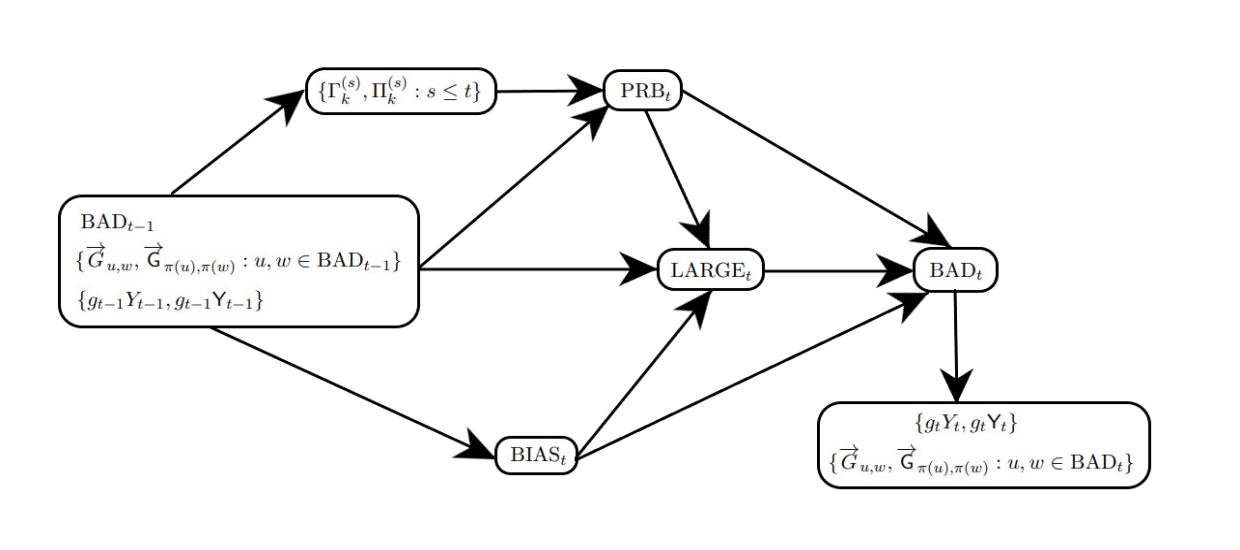
Figure 1: Logic of the definition

Let $\mathcal{T}_{-1}=\{|\mathrm{BAD}_{-1}|\leq(4nK_{0}^{2}\vartheta_{\chi}+\sqrt{n/\hat{q}(1-\hat{q})}+n^{1-\frac{2}{\log\log\log n}})\}$, and for $t\geq 0$ let $\mathcal{T}_{t}$ be the event such that

$$|\mathrm{BAD}_{t}|\leq e^{30(t+1)(\log\log n)^{20}}\vartheta^{-3t}(4nK_{0}^{2}\vartheta_{\chi}+\sqrt{n/\hat{q}(1-\hat{q})}+n^{1-\frac{2}{\log\log\log n}})\,,$$ (3.13)

$$\mbox{and }\mathrm{LARGE}_{t}^{(\log n)}=\emptyset\,.$$

By Lemma 2.1 and the fact that $t\leq 2\log\log\log n$, we have $|\mathrm{BAD}_{t}|\ll n\vartheta^{10}\Delta_{t}^{10}$ on the event $\mathcal{T}_{t}$. Our hope is that, on the one hand $\mathcal{T}_{t}$ occurs typically (as stated in Proposition 3.2 below) so that the number of “bad” vertices is under control, and on the other hand on $\mathcal{T}_{t}$ most of vertices can be dealt with by techniques of Gaussian projection which then allows to control the conditional distribution.

Proposition 3.2.

We have $\mathbb{P}(\cap_{0\leq t\leq t^{*}}\mathcal{T}_{t}\cap\mathcal{E}_{t})=1-o(1)$.

In Section 3.6, we will prove Proposition 3.2 via induction.

3.2 Preliminaries on probability and linear algebra

In this subsection we collect some standard lemmas on probability and linear algebra that will be useful for our further analysis.

The following version of Bernstein’s inequality appeared in [18, Theorem 1.4].

Lemma 3.3.

(Bernstein’s inequality). Let $X=\sum_{i=1}^{m}X_{i}$, where $X_{i}$’s are independent random variables such that $|X_{i}|\leq K$ almost surely. Then, for $s>0$ we have

$$\mathbb{P}(|X-\mathbb{E}[X]|>s)\leq 2\exp\Big{\{}-\frac{s^{2}}{2(\sigma^{2}+Ks/3)}\Big{\}}\,,$$

where $\sigma^{2}=\sum_{i=1}^{m}\mathrm{Var}(X_{i})$ is the variance of $X$.

We will also use Hanson-Wright inequality (see [29, 47, 23] and see [42, Theorem 1.1]), which is useful in controlling the quadratic form of sub-Gaussian random variables.

Lemma 3.4.

(Hanson-Wright Inequality). Let $X=(X_{1},\ldots,X_{m})$ be a random vector with independent components which satisfy $\mathbb{E}[X_{i}]=0$ and $\|X_{i}\|_{\psi_{2}}\leq K$ for all $1\leq i\leq m$. If $\mathrm{A}$ is an $m*m$ symmetric matrix, then for an absolute constant $c>0$ we have

$$\mathbb{P}(|X\mathrm{A}X^{*}-\mathbb{E}[X\mathrm{A}X^{*}]|>s)\leq 2\exp\Big{\{}-c\min\Big{(}\frac{s^{2}}{K^{4}\|\mathrm{A}\|^{2}_{\mathrm{HS}}},\frac{s}{K^{2}\|\mathrm{A}\|_{\mathrm{op}}}\Big{)}\Big{\}}\,.$$ (3.14)

The following is a corollary of Hanson-Wright inequality (see [16, Lemma 3.8]).

Lemma 3.5.

Let $X_{1},\ldots,X_{m},Y_{1},\ldots,Y_{m}$ be mean-zero variables with $\|X_{i}\|_{\psi_{2}},\|Y_{i}\|_{\psi_{2}}\leq K$ for all $1\leq i\leq m$. In addition, assume for all $i$ that $(X_{i},Y_{i})$ is independent with $(X_{\setminus i},Y_{\setminus i})$ where $X_{\setminus i}$ is obtained from $X$ by dropping its $i$-th component (and similarly for $Y_{\setminus i}$). Let $\mathrm{A}$ be an $m\times m$ matrix with diagonal entries being 0. Then for an absolute constant $c>0$ and for every $s>0$

$$\mathbb{P}(|X\mathrm{A}Y^{*}|>s)\leq 2\exp\Big{\{}-c\min\Big{(}\frac{s^{2}}{K^{4}\|\mathrm{A}\|^{2}_{\mathrm{HS}}},\frac{s}{K^{2}\|\mathrm{A}\|_{\mathrm{op}}}\Big{)}\Big{\}}\,.$$

The following inequality is standard for posterior estimation.

Lemma 3.6.

For a random variable $X$ and an event $A$ in the same probability space, we have $\mathbb{P}_{x\sim X|A}\big{(}\mathbb{P}(A|X=x)\geq\epsilon\mathbb{P}(A)\big{)}\geq 1-\epsilon$.

Proof.

We have that

$$\mathbb{P}_{x\sim X|A}\big{(}\mathbb{P}(A|X=x)= \mathbb{E}_{x\sim X}\Big{[}\frac{1}{\mathbb{P}(A)}\mathbb{P}(A|X=x)\mathbf{I}_{\{\mathbb{P}(A|X=x)\geq\epsilon\mathbb{P}(A)\}}\Big{]}$$

$$\geq \frac{1}{\mathbb{P}(A)}\mathbb{E}_{x\sim X}[\mathbb{P}(A|X=x)-\epsilon\mathbb{P}(A)]=1-\epsilon\,,$$

completing the proof of this lemma. ∎

We also need some results in linear algebra.

Lemma 3.7.

For two $m\times m$ matrices $\mathrm{A,B}$, if $\|\mathrm{(A+B)}^{-1}\|_{\mathrm{op}}\leq C,\|\mathrm{A}^{-1}\|_{\infty}\leq L$ and the entries of $\mathrm{B}$ are bounded by $\frac{K}{m}$, then $\|\mathrm{(A+B)}^{-1}\|_{\infty}\leq\max\{2KCL,2L\}$.

Proof.

It suffices to show that $\|\mathrm{(A+B)}x\|_{\infty}\geq\min\{\frac{1}{2KCL},\frac{1}{2L}\}$ for any $\|x\|_{\infty}=1$. First we consider the case when $\|x\|_{2}\geq\frac{\sqrt{m}}{2KL}$. Since $\|\mathrm{(A+B)}x\|_{2}\geq\|\mathrm{(A+B)}^{-1}\|_{\mathrm{op}}^{-1}\|x\|_{2}\geq C^{-1}\|x\|_{2}$, we get $\|\mathrm{(A+B)}x\|^{2}_{\infty}\geq\frac{\|\mathrm{(A+B)}x\|^{2}_{2}}{m}\geq\frac{1}{4K^{2}C^{2}L^{2}}$. Then we consider the case when $\|x\|_{2}\leq\frac{\sqrt{m}}{2KL}$. In this case $\|x\|_{1}\leq\frac{m}{2KL}$. Thus, $\|\mathrm{A}x\|_{\infty}\geq\|\mathrm{A}^{-1}\|_{\infty}^{-1}\|x\|_{\infty}\geq L^{-1}$ and $\|\mathrm{B}x\|_{\infty}\leq\frac{K}{m}\|x\|_{1}\leq(2L)^{-1}$. Therefore, $\|\mathrm{(A+B)}x\|_{\infty}\geq\|\mathrm{A}x\|_{\infty}-\|\mathrm{B}x\|_{\infty}\geq\frac{1}{2L}$, as desired. ∎

Lemma 3.8.

For an $m\times m$ matrix $\mathrm{A}$, suppose that there exist two partitions of $\{1,\ldots,m\}=\sqcup_{k=1}^{K}\mathcal{I}_{k}=\sqcup_{k=1}^{K}\mathcal{J}_{k}$ with $|\mathcal{I}_{k}|,|\mathcal{J}_{k}|\leq D$ (for $1\leq k\leq K$) such that $|\mathrm{A}_{a,b}|\leq\delta$ for $1\leq k\leq K$ and $(a,b)\in\mathcal{I}_{k}\times\mathcal{J}_{k}$, and that $\sum_{k\neq l}\sum_{(a,b)\in\mathcal{I}_{k}\times\mathcal{J}_{l}}\mathrm{A}_{a,b}^{2}\leq C^{2}$. Then we have $\|\mathrm{A}\|_{\mathrm{op}}\leq D\delta+C$.

Proof.

Define $\mathrm{A}^{\mathrm{diag}}_{a,b}=\mathrm{A}_{a,b}$ for $(a,b)\in\mathcal{I}_{k}\times\mathcal{J}_{k}$, and $\mathrm{A}^{\mathrm{diag}}_{a,b}=0$ otherwise. Then, there exist two permutation matrices $\mathrm{Q_{1},Q_{2}}$ such that $\mathrm{Q}_{1}\mathrm{A}^{\mathrm{diag}}\mathrm{Q}_{2}=\mathrm{diag}(\mathrm{A}_{k})_{1\leq k\leq K}$ is a block-diagonal matrix, where $\mathrm{A}_{k}$ is a matrix with size $|\mathcal{I}_{k}|*|\mathcal{J}_{k}|$, and entries bounded by $\delta$. Thus $\|\mathrm{A}^{\mathrm{diag}}\|_{\mathrm{op}}=\max_{1\leq k\leq K}\|\mathrm{A}_{k}\|_{\mathrm{op}}\leq D\delta$. Also we have $\|\mathrm{A}-\mathrm{A}^{\mathrm{diag}}\|_{\mathrm{op}}^{2}\leq\|\mathrm{A}-\mathrm{A}^{\mathrm{diag}}\|_{\mathrm{HS}}^{2}\leq C^{2}$, and thus the result follows from the triangle inequality. ∎

3.3 Analysis of initialization

In this subsection we analyze the initialization. We will prove a concentration result for $\aleph^{(a)}_{k},\Upsilon^{(a)}_{k}$ for $1\leq a\leq\chi+1,1\leq k\leq K_{0}$ in Lemma 3.13, which then implies that $\mathbb{P}(\mathcal{E}_{0})=1-o(1)$ as in Lemma 3.14. As preparations, we first collect a few technical estimates on binomial variables.

Lemma 3.9.

For $m\ll N\ll p^{-1}$ and $l=\Theta(1)$, we have

$$\mathbb{P}(\mathrm{Bin}(N+m,p)\geq l)-\mathbb{P}(\mathrm{Bin}(N,p)\geq l)\leq\frac{2ml}{N}\mathbb{P}(\mathrm{Bin}(N,p)\geq l)\,.$$

Proof.

The left hand side equals to $\sum_{k=1}^{l}\mathbb{P}(\mathrm{Bin}(m,p)=k)*\mathbb{P}(l>\mathrm{Bin}(N,p)\geq l-k)$. Since $mp\ll 1$, a straightforward computation yields that $\mathbb{P}(\mathrm{Bin}(m,p)\geq k)\sim\frac{(mp)^{k}}{k!}$ for any fixed $k$. Since $Np\ll 1$, we also have that $\frac{\mathbb{P}(\mathrm{Bin}(N,p)\geq l-k)}{\mathbb{P}(\mathrm{Bin}(N,p)\geq l)}\sim\frac{l!}{(l-k)!}(Np)^{-k}$. Thus,

$$\frac{\mathbb{P}(\mathrm{Bin}(N+m,p)\geq l)-\mathbb{P}(\mathrm{Bin}(N,p)\geq l)}{\mathbb{P}(\mathrm{Bin}(N,p)\geq l)}\leq 1.5\sum_{k=1}^{l}\frac{l!}{(l-k)!}(Np)^{-k}\cdot\frac{1}{k!}(mp)^{k}\leq\frac{2ml}{N},$$

which yields the desired bound. ∎

Corollary 3.10.

For $m\ll N,M\ll p^{-1}$ and $l=\Theta(1)$, we have

$$\mathbb{P}(\mathrm{CorBin}(N+m,N+m,p;M+m,\rho)\geq(l,l))-\mathbb{P}(\mathrm{CorBin}(N,N,p;M,\rho)\geq(l,l))$$

$$\leq\frac{4lm}{N}\mathbb{P}(\mathrm{Bin}(N,p)\geq l)\,.$$

Proof.

Let $(X,Y)\overset{d}{=}\mathrm{CorBin}(N,N,p;M,\rho)$ and $(U,U^{\prime})\overset{d}{=}\mathrm{CorBin}(m,m,p;m,\rho)$ be such that $(X,Y)$ is independent of $(U,U^{\prime})$. Then the left hand side (in the corollary-statement) equals to

$$\mathbb{P}(X+U,Y+U^{\prime}\geq l)-\mathbb{P}(X,Y\geq l)\leq\mathbb{P}(X+U\geq l>X)+\mathbb{P}(Y+U^{\prime}\geq l>Y)$$

$$= 2(\mathbb{P}(\mathrm{Bin}(N+m,p)\geq l)-\mathbb{P}(\mathrm{Bin}(N,p)\geq l))\leq\frac{4lm}{N}\mathbb{P}(\mathrm{Bin}(N,p)\geq l)\,,$$

where the last inequality follows from Lemma 3.9. This gives the desired bound. ∎

Lemma 3.11.

For all $N\gg 1,M,m,l\in\mathbb{N}$ and $p,\epsilon>0$ we have

$$\mathbb{P}(\mathrm{Bin}(N+m,p)\geq l)-\mathbb{P}(\mathrm{Bin}(N,p)\geq l)\lesssim\epsilon^{2}+\big{(}mp+\epsilon^{-1}\sqrt{mp(1-p)}\big{)}\frac{\log N}{\sqrt{Np(1-p)}}\,.$$

Proof.

Writing $Q=mp+\epsilon^{-1}\sqrt{mp(1-p)}$, we have that the left hand side is bounded by $\mathbb{P}(\mathrm{Bin}(m,p)\geq Q)+\mathbb{P}(l-Q<\mathrm{Bin}(N,p)<l)$. Applying Chebyshev’s inequality, we have $\mathbb{P}(\mathrm{Bin}(m,p)\geq Q)\leq\epsilon^{2}$. In addition, we have

$$\mathbb{P} (l-Q<\mathrm{Bin}(N,p)<l)\leq Q\max_{k>0}\{\mathbb{P}(\mathrm{Bin}(N,p)=k)\}$$

$$\leq Q\cdot\max_{k\in\{[Np],[Np]+1\},k\neq 0}\Big{\{}\binom{N}{k}p^{k}(1-p)^{N-k}\Big{\}}\lesssim\frac{Q\log N}{\sqrt{Np(1-p)}}\,,$$ (3.15)

where $[Np]=\max\{r:r\leq Np\}$. Here the last inequality above can be verified as follows: if $Np(1-p)=O(1)$, then $\frac{\log N}{\sqrt{Np(1-p)}}\gg 1$ (and thus the bound holds); if $Np(1-p)\gg 1$, then by Sterling’s formula we have $\binom{N}{k}p^{k}(1-p)^{N-k}=O(\frac{\log N}{\sqrt{Np(1-p)}})$, as desired. ∎

Corollary 3.12.

For $N\gg 1,M,m_{1},m_{2}=o(N),l\in\mathbb{N}$ and $p,\epsilon>0$, we have

$$\mathbb{P}(\mathrm{CorBin}(N+m_{1},N+m_{1},p;M+m_{2},\rho)\geq(l,l))-\mathbb{P}(\mathrm{CorBin}(N,N,p;M,\rho)\geq(l,l))$$

$$\lesssim \epsilon^{2}+(2m_{1}p+4\epsilon^{-1}\sqrt{m_{1}p(1-p)}+4\epsilon^{-1}\sqrt{m_{2}p(1-p)})\frac{\log N}{\sqrt{Np(1-p)}}\,.$$

Proof.

Let $(X,Y)\overset{d}{=}\mathrm{CorBin}(N-m_{2},N-m_{2},p;M,\rho)$, $(Z,Z^{\prime})\overset{d}{=}\mathrm{CorBin}(m_{2},m_{2},p;0,\rho)$, $(W,W^{\prime})\overset{d}{=}\mathrm{CorBin}(m_{2},m_{2},p;m_{2},\rho)$ and $(U,U)^{\prime}\overset{d}{=}\mathrm{CorBin}(m_{1},m_{1},p;0,\rho)$ be independent pairs of variables. Let $Q_{1}=m_{1}p+2\epsilon^{-1}\sqrt{m_{1}p(1-p)}$ and $Q_{2}=2\epsilon^{-1}\sqrt{m_{2}p(1-p)}$. Then the difference of probabilities in the statement is equal to

$$\mathbb{P}(X+U+W,Y+U^{\prime}+W^{\prime}\geq l)-\mathbb{P}(X+Z,Y+Z^{\prime}\geq l)$$

$$\leq \mathbb{P}(X+U+W\geq l>X+Z)+\mathbb{P}(Y+U^{\prime}+W^{\prime}\geq l>Y+Z^{\prime})$$

$$\leq 2\big{(}\mathbb{P}(|W-Z|>Q_{2})+\mathbb{P}(U>Q_{1})+\mathbb{P}(l-Q_{1}-Q_{2}\leq X+Z<l)\big{)}$$

$$\lesssim 4\epsilon^{2}+2(Q_{1}+Q_{2})(\log N)/\sqrt{Np(1-p)}\,,$$

where the last transition follows from Chebyshev’s inequality and (3.3). ∎

Recall (2.4). Define

$$\Lambda_{a}=100^{a}(n\hat{q})^{-\frac{1}{2}}(\log n)\vartheta_{a}\mbox{ for }0\leq a\leq\chi\,.$$ (3.16)

Lemma 3.13.

The following hold with probability $1-o(1)$ for all $0\leq a\leq\chi$:
(1) $\Big{|}\frac{|\aleph^{(a)}_{k}|}{n}-\vartheta_{a}\Big{|},\Big{|}\frac{|\Upsilon^{(a)}_{k}|}{n}-\vartheta_{a}\Big{|}\leq\Lambda_{a}$ for $1\leq k\leq K_{0}$;
(2) $\Big{|}\frac{|\aleph^{(a)}_{k}\cap\aleph^{(a)}_{l}|}{n}-\vartheta_{a}^{2}\Big{|},\Big{|}\frac{|\Upsilon^{(a)}_{k}\cap\Upsilon^{(a)}_{l}|}{n}-\vartheta_{a}^{2}\Big{|},\Big{|}\frac{|\pi(\aleph^{(a)}_{k})\cap\Upsilon^{(a)}_{l}|}{n}-\vartheta_{a}^{2}\Big{|}\leq\Lambda_{a}$ for $1\leq k\neq l\leq K_{0}$;
(3) $\Big{|}\frac{|\pi(\aleph^{(a)}_{k})\cap\Upsilon^{(a)}_{k}|}{n}-\varsigma_{a}\Big{|}\leq\Lambda_{a}$ for $1\leq k\leq K_{0}$.

Proof.

The proof is by induction on $a$. The base case for $a=0$ is trivial. Now suppose that Item (1), (2) and (3) hold up to some $a\leq\chi-1$ and we wish to prove that (1), (2) and (3) hold with probability $1-o(1)$ for $a+1$. To this end, applying (2.1) and Lemma 2.1 we have $\vartheta_{a}=\Theta(n^{-1}(n\hat{q})^{\chi-1})\ll\frac{1}{n\hat{q}}$. Recall the definition of $\mathrm{REV}^{(a)}$ as in (3.3), which records the collection of vertices explored by our algorithm. By the induction hypothesis we know

$$|\mathrm{REV}^{(a)}|\leq 4K_{0}\vartheta_{a}n\ll\Lambda_{a+1}n\,,$$ (3.17)

where the last transition follows from Lemma 2.1. Thus, it suffices to control the concentration of $|\aleph^{(a+1)}_{k}\setminus\mathrm{REV}^{(a)}|$ in order to control that for $|\aleph^{(a+1)}_{k}|$. Note that

$$\frac{|\aleph^{(a+1)}_{k}\setminus\mathrm{REV}^{(a)}|}{n}-\vartheta_{a+1}=\frac{1}{n}\sum_{u\in V\setminus\mathrm{REV}^{(a)}}\Big{(}\mathbf{I}_{\{u\in\aleph^{(a+1)}_{k}\}}-\vartheta_{a+1}\Big{)}+O(\vartheta_{a+1}\vartheta_{a})\,,$$

where $\vartheta_{a+1}\vartheta_{a}\ll\vartheta_{a+1}/n\hat{q}\ll\Lambda_{a+1}$ by Lemma 2.1. Since the indicators in the above sum are measurable with respect to $\{\overrightarrow{G}_{v,u}:v\in\aleph^{(a)}_{k}\}$, we see that conditioned on a realization of $\{\aleph^{(a)}_{k},\Upsilon^{(a)}_{k}\}$ we have that $\{\mathbf{I}_{\{u\in\aleph^{(a+1)}_{k}\}}:u\in V\setminus\mathrm{REV}^{(a)}\}$ is a collection of i.i.d. Bernoulli random variables with parameter given by

$$p^{(a+1)}_{k}=\mathbb{P}(u\in\aleph^{(a+1)}_{k})=\mathbb{P}(\mathrm{Bin}(|\aleph^{(a)}_{k}|,\hat{q})\geq 1)\,.$$

By the induction hypothesis, we have $\big{|}|\aleph^{(a)}_{k}|-n\vartheta_{a}\big{|}\leq n\Lambda_{a}$. Combined with Lemma 3.9, it yields that

$$\big{|}\vartheta_{a+1}-p^{(a+1)}_{k}\big{|}\leq\big{|}\mathbb{P}\big{(}\mathrm{Bin}(n\vartheta_{a},\hat{q})\geq 1\big{)}-\mathbb{P}\big{(}\mathrm{Bin}(n\vartheta_{a}+n\Lambda_{a},\hat{q})\geq 1\big{)}\big{|}$$

$$\leq \frac{2n\Lambda_{a}}{n\vartheta_{a}}\mathbb{P}(\mathrm{Bin}(n\vartheta_{a},\hat{q})\geq 1)\overset{\eqref{equ-def-iter-vartheta-varsigma},\eqref{equ-def-Lambda}}{\leq}\frac{1}{10}\Lambda_{a+1}\,.$$ (3.18)

Thus, we may apply Lemma 3.3 and get that

$$\mathbb{P}\Big{(}\Big{|}\frac{|\aleph^{(a+1)}_{k}|}{n}-\vartheta_{a+1}\Big{|}>\Lambda_{a+1}\Big{)}\overset{\eqref{eq-REV-approximation}}{\leq}\mathbb{P}\Big{(}\Big{|}\frac{|\aleph^{(a+1)}_{k}\setminus\mathrm{REV}^{(a)}|}{n}-\vartheta_{a+1}\Big{|}>\frac{9}{10}\Lambda_{a+1}\Big{)}$$

$$\overset{\eqref{equ-bound-p-a+1-minus-vartheta-a+1}}{\leq} \mathbb{P}\Big{(}\frac{1}{n}\Big{|}\mathrm{Bin}(n-|\mathrm{REV}^{(a)}|,p^{(a+1)}_{k})-(n-|\mathrm{REV}^{(a)}|)p^{(a+1)}_{k})\Big{|}>\frac{1}{2}\Lambda_{a+1}\Big{)}$$

$$\leq 2\exp\Big{\{}-\frac{(\frac{1}{2}n\Lambda_{a+1})^{2}}{2(np^{(a+1)}_{k}+n\Lambda_{a+1}/3)}\Big{\}}\leq 2\exp\{-\hat{q}^{-1}\vartheta_{a+1}(\log n)^{2}\}\,.$$ (3.19)

Similar results hold for $\Upsilon^{(a+1)}_{k}$. We now move to Item (2). Similarly, conditioned on a realization of $\{\aleph^{(a)}_{k},\Upsilon^{(a)}_{k}\}$, we have that

$$\frac{|\aleph^{(a+1)}_{k}\cap\aleph^{(a+1)}_{l}\setminus\mathrm{REV}^{(a)}|}{n}=\frac{1}{n}\sum_{u\in V\setminus\mathrm{REV}^{(a)}}\mathbf{I}_{\{u\in\aleph^{(a+1)}_{k}\cap\aleph^{(a+1)}_{l}\}}$$

is a sum of i.i.d. Bernoulli random variables with parameter give by

$$p^{(a+1)}_{k,l}= \mathbb{P}\Big{(}u\in\aleph^{(a+1)}_{k}\cap\aleph^{(a+1)}_{l}\Big{)}=\mathbb{P}\Big{(}\sum_{w\in\aleph^{(a)}_{k}}\overrightarrow{G}_{w,u},\sum_{w\in\aleph^{(a)}_{l}}\overrightarrow{G}_{w,u}\geq 1\Big{)}\,,$$

where $\big{(}\sum_{w\in\aleph^{(a)}_{k}}\overrightarrow{G}_{w,u},\sum_{w\in\aleph^{(a)}_{l}}\overrightarrow{G}_{w,u}\big{)}\overset{d}{=}\mathrm{CorBin}(|\aleph^{(a)}_{k}|,|\aleph^{(a)}_{l}|,\hat{q};|\aleph^{(a)}_{k}\cap\aleph^{(a)}_{l}|,\hat{\rho})$. By the induction hypothesis we have $\big{|}|\aleph^{(a)}_{k}|-n\vartheta_{a}\big{|},\big{|}|\aleph^{(a)}_{k}|-n\vartheta_{a}\big{|},\big{|}|\aleph^{(a)}_{k}\cap\aleph^{(a)}_{l}|-n\vartheta_{a}^{2}\big{|}\leq n\Lambda_{a}$. In addition, by Lemma 2.1 we have $\vartheta_{a}^{2}\leq\vartheta_{a}/n\hat{q}\ll\Lambda_{a}$ and thus $|\aleph^{(a)}_{k}\cap\aleph^{(a)}_{l}|\leq 1.1n\Lambda_{a}$. Combined with Corollary 3.10, these yield that

$$\Big{|}\mathbb{P}\Big{(}u\in\aleph^{(a+1)}_{k}\cap\aleph^{(a+1)}_{l}\Big{)}-\vartheta_{a+1}^{2}\Big{|}\leq\frac{5\Lambda_{a}}{\vartheta_{a}}\vartheta_{a+1}\leq\frac{1}{10}\Lambda_{a+1}\,.$$

Applying Lemma 3.3 again, we get that

$$\mathbb{P}\Big{(}\Big{|}\frac{|\aleph^{(a+1)}_{k}\cap\aleph^{(a+1)}_{l}|}{n}-\vartheta_{a+1}^{2}\Big{|}>\Lambda_{a+1}\Big{)}$$

$$\leq \mathbb{P}\Big{(}\frac{1}{n}\Big{|}\mathrm{Bin}(n-|\mathrm{REV}^{(a)}|,p^{(a+1)}_{k,l})-(n-|\mathrm{REV}^{(a)}|)p^{(a+1)}_{k,l}\Big{|}>\frac{1}{2}\Lambda_{a+1}\Big{)}$$

$$\leq 2\exp\{-\hat{q}^{-1}\vartheta_{a+1}(\log n)^{2}\}\,.$$ (3.20)

The terms $\big{|}\frac{\aleph^{(a+1)}_{k}\cap\aleph^{(a+1)}_{l}}{n}\big{|},\big{|}\frac{\Upsilon^{(a+1)}_{k}\cap\Upsilon^{(a+1)}_{l}}{n}\big{|}$ can be bounded in the same way. We next turn to Item (3). In order to bound $\big{|}\frac{\aleph^{(a+1)}_{k}\cap\Upsilon^{(a+1)}_{k}}{n}-\varsigma_{a+1}\big{|}$, note that

$$\frac{|\aleph^{(a+1)}_{k}\cap\Upsilon^{(a+1)}_{k}\setminus\mathrm{REV}^{(a)}|}{n}-\varsigma_{a+1}=\frac{1}{n}\sum_{u\in V\setminus\mathrm{REV}^{(a)}}\Big{(}\mathbf{I}_{\{u\in\aleph^{(a+1)}_{k}\cap\Upsilon^{(a+1)}_{k}\}}-\varsigma_{a+1}\Big{)}+O(\varsigma_{a+1}\vartheta_{a})\,.$$

Given a realization of $\{\aleph^{(a)}_{k},\Upsilon^{(a)}_{k}\}$, we have $\{\mathbf{I}_{\{u\in\aleph^{(a+1)}_{k}\cap\Upsilon^{(a+1)}_{k}\}}\}$ is a collection of i.i.d. Bernoulli variables, with parameter (by Lemma 3.10 and the induction hypothesis again)

$$\Big{|}\mathbb{P}\Big{(}u\in\aleph^{(a+1)}_{k}\cap\Upsilon^{(a+1)}_{k}\Big{)}-\varsigma_{a+1}\Big{|}=\Big{|}\mathbb{P}(X,Y\geq 1)-\varsigma_{a+1}\Big{|}\leq\frac{5\Lambda_{a}}{\vartheta_{a}}\vartheta_{a+1}\leq\frac{1}{10}\Lambda_{a+1}\,,$$

where $(X,Y)\sim\mathrm{CorBin}(|\aleph^{(a)}_{k}|,|\Upsilon^{(a)}_{k}|,q;|\aleph^{(a)}_{k}\cap\Upsilon^{(a)}_{k}|;\rho)$. By Lemma 3.3 again, we get that

$$\mathbb{P}\Big{(}\Big{|}\frac{|\aleph^{(a+1)}_{k}\cap\Upsilon^{(a+1)}_{k}|}{n}-\varsigma_{a+1}\Big{|}>\Lambda_{a+1}\Big{)}$$

$$\leq \mathbb{P}\Big{(}\Big{|}\frac{|\aleph^{(a+1)}_{k}\cap\Upsilon^{(a+1)}_{k}\setminus\mathrm{REV}^{(a)}|}{n}-\varsigma_{a+1}\Big{|}>\frac{9}{10}\Lambda_{a+1}\Big{)}$$

$$\leq 2\exp\Big{\{}-\frac{(\frac{1}{2}\Lambda_{a+1}n)^{2}}{2(n\varsigma_{a+1}+n\Lambda_{a+1}/3)}\Big{\}}\leq 2\exp\{-\hat{q}^{-1}\vartheta_{a+1}(\log n)^{2}\}\,.$$ (3.21)

Combining (3.19), (3.20), and (3.21) and applying a union bound, we see that (assuming (1), (2), (3) holds for $a$) the conditional probability for (1), (2), or (3) to fail is at most $2K_{0}^{2}\exp\{-(\log n)^{2}\}$ since $\vartheta_{a+1}\geq\vartheta_{1}=\hat{q}$. Therefore, we complete the proof of Lemma 3.13 by induction (note that $\chi=O(1)$). ∎

Lemma 3.14.

We have $\mathbb{P}(\mathcal{E}_{0})=1-o(1)$.

Proof.

By Lemma 3.13, with probability $1-o(1)$ we have $|\mathrm{REV}|\leq 4K_{0}n\vartheta_{\chi}\ll n\vartheta\Delta_{0}$, where we used Lemma 2.1 and (3.1). Provided with this, it suffices to analyze $\frac{|\Gamma^{(0)}_{k}\setminus\mathrm{REV}|}{n}$, whose conditional distribution given $\{\aleph^{(a)}_{k},\Upsilon^{(a)}_{k}:1\leq k\leq K_{0},0\leq a\leq\chi\}$ is the same as the sum of $n-|\mathrm{REV}|$ i.i.d. Bernoulli variables with parameter given by

$$\mathbb{P}(u\in\Gamma^{(0)}_{k})=\mathbb{P}(\mathrm{Bin}(|\aleph^{(\chi)}_{k}|,\hat{q})\geq\mathtt{d}_{\chi})\,.$$

By Lemma 3.13 again, we have $\Big{|}|\aleph^{(\chi)}_{k}|-\vartheta_{\chi}n\Big{|}\leq n\Lambda_{\chi}$ with probability $1-o(1)$. Provided with this and applying Lemma 3.11 (with $\epsilon=\vartheta\Delta_{0}$), we get that

$$|\mathbb{P}(u\in\Gamma^{(0)}_{k})-\vartheta|\leq |\mathbb{P}(\mathrm{Bin}(\vartheta_{\chi}n+n\Lambda_{\chi},\hat{q})\geq\mathtt{d}_{\chi})-\mathbb{P}(\mathrm{Bin}(\vartheta_{\chi}n,\hat{q})\geq\mathtt{d}_{\chi})|$$

$$\leq (\vartheta\Delta_{0})^{2}+(\log n)\frac{n\Lambda_{\chi}\hat{q}+2(\vartheta\Delta_{0})^{-1}\sqrt{n\Lambda_{\chi}\hat{q}}}{\sqrt{\vartheta_{\chi}n\hat{q}}}\ll\vartheta\Delta_{0}\,,$$

where we used (3.1) and the inequalities $\frac{n\Lambda_{\chi}\hat{q}}{\sqrt{\vartheta_{\chi}n\hat{q}}}=100^{\chi}\sqrt{\vartheta_{\chi}}\log n\ll\vartheta\Delta_{0}/\log n$ (by Lemma 2.1) as well as $\frac{(\vartheta\Delta_{0})^{-1}\sqrt{n\Lambda_{\chi}\hat{q}}}{\sqrt{\vartheta_{\chi}n\hat{q}}}=(n\hat{q})^{-\frac{1}{4}}(\vartheta\Delta_{0})^{-1}\ll\vartheta\Delta_{0}/\log n$. By Lemma 3.3,

$$\mathbb{P}\Big{(}\Big{|}\frac{|\Gamma^{(0)}_{k}|}{n}-\vartheta\Big{|}>\vartheta\Delta_{0}\Big{)}=\mathbb{P}\Big{(}\Big{|}\frac{|\Gamma^{(0)}_{k}\setminus\mathrm{REV}|}{n}-\vartheta\Big{|}>\frac{9}{10}\vartheta\Delta_{0}\Big{)}$$

$$\leq \mathbb{P}\Big{(}\Big{|}\frac{1}{n}\mathrm{Bin}(n-|\mathrm{REV}|,\vartheta+o(\vartheta\Delta_{0}))-\vartheta\Big{|}>\frac{9}{10}\vartheta\Delta_{0}\Big{)}$$

$$\leq 2\exp\Big{\{}-\frac{(\frac{1}{2}\vartheta\Delta_{0}n)^{2}}{2(n\vartheta+\vartheta\Delta_{0}n/3)}\Big{\}}\leq 2\exp\{-2\vartheta\Delta_{0}^{2}n\}\,.$$ (3.22)

We can obtain the concentration for $\frac{|\Pi^{(0)}_{k}|}{n}$, $\frac{|\Gamma^{(0)}_{k}\cap\Gamma^{(0)}_{l}|}{n}$, $\frac{|\Pi^{(0)}_{k}\cap\Pi^{(0)}_{l}|}{n}$ and $\frac{|\pi(\Gamma^{(0)}_{k})\cap\Pi^{(0)}_{l}|}{n}$ similarly. For instance, for $\frac{|\pi(\Gamma^{(0)}_{k})\cap\Pi^{(0)}_{l}|}{n}$, we note that given $\{\aleph^{(a)}_{k},\Upsilon^{(a)}_{k}:1\leq k\leq K_{0},0\leq a\leq\chi\}$,

$$\frac{|\Gamma^{(0)}_{k}\cap\pi^{-1}(\Pi^{(0)}_{l})\setminus\mathrm{REV}|}{n}=\sum_{u\in V\setminus\mathrm{REV}}\mathbf{I}_{\{u\in\Gamma^{(0)}_{k}\cap\pi^{-1}(\Pi^{(0)}_{l})\}}$$

is a sum of i.i.d. Bernoulli variables with parameter given by

$$\mathbb{P}(u\in\Gamma^{(0)}_{k}\cap\pi^{-1}(\Pi^{(0)}_{l}))=\mathbb{P}(\mathrm{CorBin}(|\aleph^{(\chi)}_{k}|,|\Upsilon^{(\chi)}_{l}|,\hat{q};|\aleph^{(0)}_{k}\cap\pi^{-1}(\Upsilon^{(0)}_{l})|,\hat{\rho})\geq(\mathtt{d}_{\chi},\mathtt{d}_{\chi}))\,.$$

By Lemma 3.13, we have $\big{|}|\aleph^{(\chi)}_{k}|-n\vartheta_{\chi}\big{|},\big{|}|\Upsilon^{(\chi)}_{k}|-n\vartheta_{\chi}\big{|},\big{|}|\aleph^{(0)}_{k}\cap\pi^{-1}(\Upsilon^{(0)}_{l})|-n\varsigma_{\chi}\big{|}\leq n\Lambda_{\chi}$ with probability $1-o(1)$. Provided with this and applying Corollary 3.12 again (with $\epsilon=\vartheta\Delta_{0}$), we get that $\mathbb{P}(u\in\Gamma^{(0)}_{k}\cap\pi^{-1}(\Pi^{(0)}_{l}))=\varsigma+o(\vartheta\Delta_{0})$. Thus we can obtain a similar concentration bound using Lemma 3.3. We omit further details due to similarity.

By (3.22) (and its analogues) and a union bound, we deduce that

$$\mathbb{P}(\mathcal{E}_{0}^{c})\leq 20K_{0}^{2}\exp\{-2\vartheta\Delta_{0}^{2}n\}=o(1)\,,$$ (3.23)

where for the last step we recalled (3.1) and Lemma 2.1. This completes the proof. ∎

3.4 Density comparison

Our proof of the admissibility along the iteration relies on a direct comparison of the smoothed Bernoulli density and the Gaussian density, which then allows us to use the techniques developed in [16] for correlated Gaussian Wigner matrices. Recall (3.4), (3.6) and (3.10). Our main result in this subsection is Lemma 3.16 below, and we need to introduce more notations before its statement.

For a random variable $X$ and a $\sigma$-field $\mathcal{F}$, we denote by $p_{\{X\mid\mathcal{F}\}}$ the conditional density of $X$ given $\mathcal{F}$. For a realization $\Xi_{t}=\{\xi^{(s)}_{k},\zeta^{(s)}_{k}:s\leq t,1\leq k\leq K_{s}\}$ for $\{\Gamma^{(s)}_{k},\Pi^{(s)}_{k}:s\leq t,1\leq k\leq K_{s}\}$ and a realization $\mathrm{B}_{t-1}$ for $\mathrm{BAD}_{t-1}$, we define vector-valued functions $\varphi^{(s)}_{v}(\Xi_{t},\mathrm{B}_{t-1}),\psi^{(s)}_{v}(\Xi_{t},\mathrm{B}_{t-1})$ for $v\not\in\mathrm{B}_{t-1}$ and $0\leq s\leq t$, where for $1\leq k\leq K_{s}$ the $k$-th component is given by

$$\varphi^{(s)}_{v,k}(\Xi_{t},\mathrm{B}_{t-1}) =\frac{1}{\sqrt{(\mathfrak{a}_{s}-\mathfrak{a}_{s}^{2})n\hat{q}(1-\hat{q})}}\sum_{u\not\in\mathrm{B}_{t-1}}(\mathbf{I}_{u\in\xi^{(s)}_{k}}-\mathfrak{a}_{s})(\overrightarrow{G}_{v,u}-\hat{q})\,,$$ (3.24)

$$\psi^{(s)}_{v,k}(\Xi_{t},\mathrm{B}_{t-1}) =\frac{1}{\sqrt{(\mathfrak{a}_{s}-\mathfrak{a}_{s}^{2})n\hat{q}(1-\hat{q})}}\sum_{u\not\in\mathrm{B}_{t-1}}(\mathbf{I}_{u\in\xi^{(s)}_{k}}-\mathfrak{a}_{s})\overrightarrow{Z}_{v,u}\,.$$

Similarly, we define $\varphi^{(s)}_{\pi(v)}(\Xi_{t},\mathrm{B}_{t-1}),\psi^{(s)}_{\pi(v)}(\Xi_{t},\mathrm{B}_{t-1})$ where for $1\leq k\leq K_{s}$ the $k$-th component is given by

$$\varphi^{(s)}_{\pi(v),k}(\Xi_{t},\mathrm{B}_{t-1}) =\frac{1}{\sqrt{(\mathfrak{a}_{s}-\mathfrak{a}_{s}^{2})n\hat{q}(1-\hat{q})}}\sum_{u\not\in\mathrm{B}_{t-1}}(\mathbf{I}_{\pi(u)\in\zeta^{(s)}_{k}}-\mathfrak{a}_{s})(\overrightarrow{\mathsf{G}}_{\pi(v),\pi(u)}-\hat{q})\,,$$ (3.25)

$$\psi^{(s)}_{\pi(v),k}(\Xi_{t},\mathrm{B}_{t-1}) =\frac{1}{\sqrt{(\mathfrak{a}_{s}-\mathfrak{a}_{s}^{2})n\hat{q}(1-\hat{q})}}\sum_{u\not\in\mathrm{B}_{t-1}}(\mathbf{I}_{\pi(u)\in\zeta^{(s)}_{k}}-\mathfrak{a}_{s})\overrightarrow{\mathsf{Z}}_{\pi(v),\pi(u)}\,.$$

In addition, define $\mathrm{B}_{t}=\mathrm{B}_{t}(\Xi_{t},\mathrm{B}_{t-1},\overrightarrow{G},\overrightarrow{\mathsf{G}},W,\mathsf{W})$ to be the corresponding realization of $\mathrm{BAD}_{t}$, i.e., $\mathrm{B}_{t}$ is the collection of vertices satisfying either of (3.5), (3.8), (3.9) and (3.11) with $(\Gamma^{(s)}_{k},\Pi^{(s)}_{k})$ replaced by $(\xi^{(s)}_{k},\zeta^{(s)}_{k})$ and $\mathrm{BAD}_{t-1}$ replaced by $\mathrm{B}_{t-1}$. Define a random vector $\mathbf{X}^{\leq t}=\mathbf{X}^{\leq t}(\mathrm{B}_{t},\mathrm{B}_{t-1})$ by

$$\mathbf{X}^{\leq t}(s,k,v)=W^{(s)}_{v}(k)+\langle\eta^{(s)}_{k},\varphi^{(s)}_{v}\rangle\mbox{ and }\mathbf{X}^{\leq t}(s,k,\pi(v))=\mathsf{W}^{(s)}_{\pi(v)}(k)+\langle\eta^{(s)}_{k},\varphi^{(s)}_{\pi(v)}\rangle$$

where $0\leq s\leq t,1\leq k\leq\frac{K_{s}}{12}$, and $v\not\in\mathrm{B}_{t-1}$ when $s<t$, and $v\not\in\mathrm{B}_{t}$ when $s=t$. Define $\mathbf{Y}^{\leq t}$ similarly by replacing $\varphi^{(s)}_{v}$ with $\psi^{(s)}_{v}$ and replacing $W,\mathsf{W}$ with $\tilde{W},\tilde{\mathsf{W}}$. Let $\mathbf{X}^{=t}$ be the vector obtained from $\mathbf{X}^{\leq t}$ by keeping its coordinates with $s=t$, and let $\mathbf{X}^{<t}$ be the vector obtained from $\mathbf{X}^{\leq t}$ by keeping its coordinates with $s<t$. Define $\mathbf{Y}^{=t}$ and $\mathbf{Y}^{<t}$ with respect to $\mathbf{Y}^{\leq t}$ similarly. We also define $\hat{\mathbf{X}}^{\leq t}(s,k,v)=\mathbf{X}^{\leq t}(s,k,v)-W^{(s)}_{v}(k)$ and $\hat{\mathbf{Y}}^{\leq t}(s,k,v)=\mathbf{Y}^{\leq t}(s,k,v)-\tilde{W}^{(s)}_{v}(k)$. Also, define $(\overrightarrow{G}_{\mathrm{B}},\overrightarrow{\mathsf{G}}_{\mathrm{B}})=(\overrightarrow{G}_{u,w},\overrightarrow{\mathsf{G}}_{\pi(u),\pi(w)}:u\mbox{ or }w\in\mathrm{B}_{t-1})$, and define $(\overrightarrow{G}_{\setminus\mathrm{B}},\overrightarrow{\mathsf{G}}_{\setminus\mathrm{B}})=(\overrightarrow{G}_{u,w},\overrightarrow{\mathsf{G}}_{\pi(u),\pi(w)}:u,w\not\in\mathrm{B}_{t-1})$. Denote by $(\overrightarrow{g}_{\mathrm{B}},\overrightarrow{\mathsf{g}}_{\mathrm{B}})$ be the realization of $(\overrightarrow{G}_{\mathrm{B}},\overrightarrow{\mathsf{G}}_{\mathrm{B}})$. For any fixed realization $(\Xi_{t},\mathrm{B}_{t},\mathrm{B}_{t-1},\overrightarrow{g}_{\mathrm{B}},\overrightarrow{\mathsf{g}}_{\mathrm{B}})$, we further define $\mathtt{p}_{\{\mathbf{X}^{\leq t}\}}(x^{\leq t})=p({x}^{\leq t},\Xi_{t},\mathrm{B}_{t},\mathrm{B}_{t-1},\overrightarrow{g}_{\mathrm{B}},\overrightarrow{\mathsf{g}}_{\mathrm{B}})$ to be the conditional density as follows:

$$\mathtt{p}_{\{\mathbf{X}^{\leq t}\}}(x^{\leq t})=p_{\{\mathbf{X}^{\leq t}\mid\mathrm{BAD}_{t}=\mathrm{B}_{t};\mathrm{BAD}_{t-1}=\mathrm{B}_{t-1};(\overrightarrow{G}_{\mathrm{B}},\overrightarrow{\mathsf{G}}_{\mathrm{B}})=(\overrightarrow{g}_{\mathrm{B}},\overrightarrow{\mathsf{g}}_{\mathrm{B}})\}}(x^{\leq t})\,,$$

where the support of $x^{\leq t}$ is consistent with the choice of $(\mathrm{B}_{t},\mathrm{B}_{t-1})$ (i.e., $x^{\leq t}$ is a legitimate realization for $\mathbf{X}^{\leq t}=\mathbf{X}^{\leq t}(\mathrm{B}_{t},\mathrm{B}_{t-1})$). Note that when defining the conditional density above, we did not condition on $\{\Gamma^{(s)}_{k},\Pi^{(s)}_{k}:s\leq t,1\leq k\leq K_{s}\}=\Xi_{t}$; rather, $\Xi_{t}$ played its role in the definitions (3.24) and (3.25). Define $\mathtt{p}_{\{\mathbf{Y}^{\leq t}\}}({x}^{\leq t})$ similarly but with respect to $\mathbf{Y}^{\leq t}$. For the purpose of truncation later, we say a realization $(\mathrm{B}_{t},\mathrm{B}_{t-1})$ for $(\mathrm{BAD}_{t},\mathrm{BAD}_{t-1})$ is an amenable set-realization, if

$$\mathbb{P}(\mathrm{BAD}_{t}=\mathrm{B}_{t},\mathrm{BAD}_{t-1}=\mathrm{B}_{t-1})\geq\exp\{-n\Delta_{t}^{9}\}\,.$$ (3.26)

Also, we say $(\overrightarrow{g}_{\mathrm{B}},\overrightarrow{\mathsf{g}}_{\mathrm{B}})$ is an amenable bias-realization with respect to $(\mathrm{B}_{t},\mathrm{B}_{t-1})$, if

$$\mathbb{P}(\mathrm{BAD}_{t}=\mathrm{B}_{t},\mathrm{BAD}_{t-1}=\mathrm{B}_{t-1}|(\overrightarrow{G}_{\mathrm{B}},\overrightarrow{\mathsf{G}}_{\mathrm{B}})=(\overrightarrow{g}_{\mathrm{B}},\overrightarrow{\mathsf{g}}_{\mathrm{B}}))\geq\exp\{-n\Delta_{t}^{8}\}\,.$$ (3.27)

In addition, we say a realization $x^{\leq t}=x^{\leq t}(\mathrm{B}_{t},\mathrm{B}_{t-1})$ for $\mathbf{X}^{\leq t}(\mathrm{B}_{t},\mathrm{B}_{t-1})$ is an amenable variable-realization with respect to $(\mathrm{B}_{t},\mathrm{B}_{t-1}),(\overrightarrow{g}_{\mathrm{B}},\overrightarrow{\mathsf{g}}_{\mathrm{B}})$, if it is consistent with the choice of $(\mathrm{B}_{t},\mathrm{B}_{t-1})$ and $(\overrightarrow{g}_{\mathrm{B}},\overrightarrow{\mathsf{g}}_{\mathrm{B}})$, and (below the vector $x^{<t}$ is obtained by keeping the coordinates of $x^{\leq t}$ with $s<t$)

$$\|x^{\leq t}\|_{\infty}\leq 2(\log n)n^{\frac{1}{\log\log\log n}},$$ (3.28)

$$\frac{p_{\{\mathbf{Y}^{<t}|\mathrm{BAD}_{t}=\mathrm{B}_{t},\mathrm{BAD}_{t-1}=\mathrm{B}_{t-1},(\overrightarrow{G}_{\mathrm{B}},\overrightarrow{\mathsf{G}}_{\mathrm{B}})=(\overrightarrow{g}_{\mathrm{B}},\overrightarrow{\mathsf{g}}_{\mathrm{B}})\}}(x^{<t})}{p_{\{\mathbf{X}^{<t}|\mathrm{BAD}_{t}=\mathrm{B}_{t},\mathrm{BAD}_{t-1}=\mathrm{B}_{t-1},(\overrightarrow{G}_{\mathrm{B}},\overrightarrow{\mathsf{G}}_{\mathrm{B}})=(\overrightarrow{g}_{\mathrm{B}},\overrightarrow{\mathsf{g}}_{\mathrm{B}})\}}(x^{<t})}\leq\exp\{n\Delta_{t}^{10}\}\,,$$ (3.29)

and $$\frac{p_{\{\mathbf{Y}^{\leq t}|\mathrm{BAD}_{t}=\mathrm{B}_{t},\mathrm{BAD}_{t-1}=\mathrm{B}_{t-1},(\overrightarrow{G}_{\mathrm{B}},\overrightarrow{\mathsf{G}}_{\mathrm{B}})=(\overrightarrow{g}_{\mathrm{B}},\overrightarrow{\mathsf{g}}_{\mathrm{B}})\}}(x^{\leq t})}{p_{\{\mathbf{X}^{\leq t}|\mathrm{BAD}_{t}=\mathrm{B}_{t},\mathrm{BAD}_{t-1}=\mathrm{B}_{t-1},(\overrightarrow{G}_{\mathrm{B}},\overrightarrow{\mathsf{G}}_{\mathrm{B}})=(\overrightarrow{g}_{\mathrm{B}},\overrightarrow{\mathsf{g}}_{\mathrm{B}})\}}(x^{\leq t})}\leq\exp\{n\Delta_{t}^{10}\}\,.$$ (3.30)

Lemma 3.15.

On the event $\mathcal{T}_{t}$, with probability $1-O(\exp\{-n\Delta_{t}^{10}\})$ we have that

• $(\mathrm{B}_{t},\mathrm{B}_{t-1})$ sampled according to $(\mathrm{BAD}_{t},\mathrm{BAD}_{t-1})$ is an amenable set-realization;

• $(\overrightarrow{g}_{\mathrm{B}},\overrightarrow{\mathsf{g}}_{\mathrm{B}})$ sampled according to $\{(\overrightarrow{G}_{\mathrm{B}},\overrightarrow{\mathsf{G}}_{\mathrm{B}})|\mathrm{BAD}_{t}=\mathrm{B}_{t},\mathrm{B}_{t-1}=\mathrm{B}_{t-1}\}$ is an amenable bias-realization with respect to $(\mathrm{B}_{t},\mathrm{B}_{t-1})$;

• $x^{\leq t}(\mathrm{B}_{t},\mathrm{B}_{t-1})$ sampled according to $\{\mathbf{X}^{\leq t}|\mathrm{BAD}_{t}=\mathrm{B}_{t};\mathrm{BAD}_{t-1}=\mathrm{B}_{t-1};(\overrightarrow{G}_{\mathrm{B}},\overrightarrow{\mathsf{G}}_{\mathrm{B}})=(\overrightarrow{g}_{\mathrm{B}},\overrightarrow{\mathsf{g}}_{\mathrm{B}})\}$ is an amenable variable-realization with respect to $(\mathrm{B}_{t},\mathrm{B}_{t-1})$ and $(\overrightarrow{g}_{\mathrm{B}},\overrightarrow{\mathsf{g}}_{\mathrm{B}})$.

Proof.

We first consider $(\mathrm{B}_{t},\mathrm{B}_{t-1})$. On $\mathcal{T}_{t}$ we have $|\mathrm{BAD}_{t}|,|\mathrm{BAD}_{t-1}|\leq n\Delta_{t}^{10}$. Note that $(\mathrm{BAD}_{t},\mathrm{B}_{t-1})$ are two subsets of $V$ each of which has at most $\binom{n}{n\Delta_{t}^{10}}$ possible values. Thus,

$$\mathbb{P}(\mathrm{BAD}_{t}\not\in\{\mbox{amenable set-realization}\};\mathcal{T}_{t})\leq\Big{(}\binom{n}{n\Delta_{t}^{10}}\Big{)}^{2}\exp\{-n\Delta_{t}^{9}\}\ll\exp\{-\tfrac{1}{2}n\Delta_{t}^{9}\}\,.$$

Given an amenable set-realization $(\mathrm{B}_{t},\mathrm{B}_{t-1})$, we now consider $(\overrightarrow{g}_{\mathrm{B}},\overrightarrow{\mathsf{g}}_{\mathrm{B}})$. By Lemma 3.6,

$$\mathbb{P}_{(\overrightarrow{g}_{\mathrm{B}},\overrightarrow{\mathsf{g}}_{\mathrm{B}})\sim\{(\overrightarrow{G}_{\mathrm{B}},\overrightarrow{\mathsf{G}}_{\mathrm{B}})|\mathrm{BAD}_{t}=\mathrm{B}_{t},\mathrm{B}_{t-1}=\mathrm{B}_{t-1}\}}\big{(}(\overrightarrow{g}_{\mathrm{B}},\overrightarrow{\mathsf{g}}_{\mathrm{B}})\mbox{ is bias-amenable}\big{)}\geq 1-\exp\{-n\Delta_{t}^{9}\}\,.$$

Finally we consider $\mathbf{X}^{\leq t}$. Combining Markov’s inequality and (define $\mathcal{A}=\{\mathrm{BAD}_{t}=\mathrm{B}_{t};\mathrm{BAD}_{t-1}=\mathrm{B}_{t-1};(\overrightarrow{G}_{\mathrm{B}},\overrightarrow{\mathsf{G}}_{\mathrm{B}})=(\overrightarrow{g}_{\mathrm{B}},\overrightarrow{\mathsf{g}}_{\mathrm{B}})\}$)

$$\mathbb{E}_{x^{\leq t}\sim\{\mathbf{X}^{\leq t}\mid\mathcal{A}\}}\Big{[}\frac{p_{\{\mathbf{Y}^{\leq t}\mid\mathcal{A}\}}(x^{\leq t})}{p_{\{\mathbf{X}^{\leq t}\mid\mathcal{A}\}}(x^{\leq t})}\Big{]}=1\,,$$

we get that conditioned on $\{\mathrm{BAD}_{t}=\mathrm{B}_{t},\mathrm{BAD}_{t-1}=\mathrm{B}_{t-1},(\overrightarrow{G}_{\mathrm{B}},\overrightarrow{\mathsf{G}}_{\mathrm{B}})=(\overrightarrow{g}_{\mathrm{B}},\overrightarrow{\mathsf{g}}_{\mathrm{B}})\}$, the (random) realization $x^{\leq t}$ for $\mathbf{X}^{\leq t}$ satisfies (3.30) with probability at least $1-\exp\{-n\Delta_{t}^{10}\}$. Similarly, the realization $x^{\leq t}$ satisfies (3.29) with probability at least $1-\exp\{-n\Delta_{t}^{10}\}$. In addition, for any $s\leq t-1$ and $v\not\in\mathrm{B}_{t-1}$, recalling that $\mathrm{B}_{t-1}$ is the realization for $\mathrm{BAD}_{t-1}$ and using $\mathcal{T}_{t-1}$, (3.8) and (3.9), we derive from the triangle inequality that

$$|\mathbf{X}^{\leq t}(s,k,v)| \leq|W^{(s)}_{k}(v)|+|\langle\eta^{(s)}_{k},g_{t-2}\varphi^{(s)}_{v}\rangle|+\sum_{a=0}^{\log n}|\langle\eta^{(s)}_{k},b_{t-1,a}\varphi^{(s)}_{v}\rangle|$$

$$\leq(3+\log n)n^{\frac{1}{\log\log\log n}}\,,$$ (3.31)

where $g_{t-2}\varphi^{(s)}_{v}(k)$ denotes the (first) expression (3.24) but the summation is taken for all $u\not\in\mathrm{BAD}_{t-2}$, $b_{t-1,0}\varphi^{(s)}_{v}$ denotes the expression (3.24) but the summation is taken for all $u\in\mathrm{LARGE}^{(0)}_{t}\cup\mathrm{BIAS}_{t}\cup\mathrm{PRB}_{t}$, and $b_{t-1,a}\varphi^{(s)}_{v}$ denotes the expression (3.24) but the summation is taken for all $u\in\mathrm{LARGE}^{(a)}_{t}$. Similarly we have $|\langle\eta^{(s)}_{k},\varphi^{(s)}_{\pi(v)}\rangle|\leq(3+\log n)n^{\frac{1}{\log\log\log n}}$. For any $v\not\in\mathrm{B}_{t}$, we in particular have $v\not\in\mathrm{LARGE}_{t}$. Thus, choosing $s=t$ in (3.8) gives that

$$|\mathbf{X}^{\leq t}(t,k,v)|\leq|W^{(t)}_{k}(v)|+|\langle\eta^{(t)}_{k},\varphi^{(t)}_{v}\rangle|\leq 2n^{\frac{1}{\log\log\log n}}\,.$$ (3.32)

In conclusion, in either case of $s<t$ or $s=t$ we can show that $\{\mathrm{BAD}_{t}=\mathrm{B}_{t},\mathrm{BAD}_{t-1}=\mathrm{B}_{t-1}\}$ implies that $|\mathbf{X}^{\leq t}(s,k,v)|,|\mathbf{X}^{\leq t}(s,k,\pi(v))|\leq(3+\log n)n^{\frac{1}{\log\log\log n}}$. Altogether, we complete the proof of the lemma. ∎

Lemma 3.16.

For $t\leq t^{*}$, on the event $\mathcal{E}_{t}\cap\mathcal{T}_{t}$, fix an amenable set-realization $(\mathrm{B}_{t},\mathrm{B}_{t-1})$, fix an amenable bias-realization $(\overrightarrow{g}_{\mathrm{B}},\overrightarrow{\mathsf{g}}_{\mathrm{B}})$ with respect to $(\mathrm{B}_{t},\mathrm{B}_{t-1})$, and fix an amenable variable-realization $x^{\leq t}$ with respect to $(\mathrm{B}_{t},\mathrm{B}_{t-1})$ and $(\overrightarrow{g}_{\mathrm{B}},\overrightarrow{\mathsf{g}}_{\mathrm{B}})$. Then we have (below the vector $x^{=t}$ is defined by keeping the coordinates of $x^{\leq t}$ such that $s=t$)

$$\frac{p_{\{\mathbf{X}^{=t}|\mathfrak{S}_{t-1};\mathrm{BAD}_{t}=\mathrm{B}_{t}\}}(x^{=t})}{p_{\{\mathbf{Y}^{=t}|\mathcal{F}_{t-1}\}}(x^{=t})}=\exp\big{\{}O\big{(}n\Delta_{t}^{5}\big{)}\big{\}}\,.$$ (3.33)

Remark 3.17.

Since $\{\mathrm{BAD}_{t}=\mathrm{B}_{t}\}$ is measurable with respect to $(\overrightarrow{G},\overrightarrow{\mathsf{G}},W,\mathsf{W})$ and thus independent of $(\overrightarrow{Z},\overrightarrow{\mathsf{Z}},\tilde{W},\tilde{\mathsf{W}})$, we have that ${p}_{\{\mathbf{Y}^{\leq t}\}}(x^{\leq t})={p}_{\{\mathbf{Y}^{\leq t}|\mathrm{BAD}_{t}=\mathrm{B}_{t}\}}(x^{\leq t})$. That is, we may add conditioning on $\mathrm{BAD}_{t}=\mathrm{B}_{t}$ in the denominator of (3.33), but this will not change its conditional density.

The key to the proof of Lemma 3.16 is the following bound on the “joint” density.

Lemma 3.18.

For $t\leq t^{*}$, on the event $\mathcal{E}_{t}\cap\mathcal{T}_{t}$, for an amenable set-realization $(\mathrm{B}_{t},\mathrm{B}_{t-1})$, and an amenable bias-realization $(\overrightarrow{g}_{\mathrm{B}},\overrightarrow{\mathsf{g}}_{\mathrm{B}})$ with respect to $(\mathrm{B}_{t},\mathrm{B}_{t-1})$ and an amenable variable-realization $x^{\leq t}$ with respect to $(\mathrm{B}_{t},\mathrm{B}_{t-1})$ and $(\overrightarrow{g}_{\mathrm{B}},\overrightarrow{\mathsf{g}}_{\mathrm{B}})$, we have

$$\frac{\mathtt{p}_{\{\mathbf{X}^{\leq t}\}}(x^{\leq t})}{\mathtt{p}_{\{\mathbf{Y}^{\leq t}\}}(x^{\leq t})},\frac{\mathtt{p}_{\{\mathbf{X}^{<t}\}}(x^{<t})}{\mathtt{p}_{\{\mathbf{Y}^{<t}\}}(x^{<t})}=\exp\big{\{}O(n\Delta_{t}^{5})\big{\}}\,.$$ (3.34)

Proof of Lemma 3.16 assuming Lemma 3.18.

Applying Lemma 3.18 for both $t$ and $t-1$, we get that

$$\frac{\mathtt{p}_{\{\mathbf{X}^{=t}|\mathbf{X}^{<t}\}}(x^{=t}|x^{<t})}{\mathtt{p}_{\{\mathbf{Y}^{=t}|\mathbf{Y}^{<t}\}}(x^{=t}|x^{<t})}=\exp\{O(n\Delta_{t}^{5})\}\,.$$

Since $p_{\{\mathbf{X}^{=t}|\mathfrak{S}_{t-1},\mathrm{BAD}_{t}=\mathrm{B}_{t}\}}(x^{=t})=\frac{\mathtt{p}_{\{\mathbf{X}^{\leq t}\}(x^{\leq t})}}{\mathtt{p}_{\{\mathbf{X}^{<t}\}(x^{<t})}}$, we complete the proof of the lemma. ∎

The rest of this subsection is devoted to the proof of Lemma 3.18. Due to similarity, we only prove it for $\frac{\mathtt{p}_{\{\mathbf{X}^{\leq t}\}}(x^{\leq t})}{\mathtt{p}_{\{\mathbf{Y}^{\leq t}\}}(x^{\leq t})}$. Also since $x^{\leq t}$ is an amenable variable-realization, the lower bound is obvious and as a result we only need to prove the upper bound. Note that $(\mathrm{BAD}_{t},\mathrm{BAD}_{t-1})=(\mathrm{BAD}_{t}(\overrightarrow{G},\overrightarrow{\mathsf{G}},W,\mathsf{W}),\mathrm{BAD}_{t-1}(\overrightarrow{G},\overrightarrow{\mathsf{G}},W,\mathsf{W}))$ is a function of $(\overrightarrow{G},\overrightarrow{\mathsf{G}},W,\mathsf{W})$. Also since $(\overrightarrow{G}_{\mathrm{B}},\overrightarrow{\mathsf{G}}_{\mathrm{B}})$ is independent with $\mathbf{X}^{\leq t}(\mathrm{B}_{t},\mathrm{B}_{t-1},W,\mathsf{W})$ and with $(\overrightarrow{G}_{\setminus\mathrm{B}},\overrightarrow{\mathsf{G}}_{\setminus\mathrm{B}},W,\mathsf{W})$, we have

$$\mathtt{p}_{\{\mathbf{X}^{\leq t}\}}(x^{\leq t})=p_{\{\mathbf{X}^{\leq t}|\bar{\mathcal{A}}\}}(x^{\leq t})\,,$$

where $\bar{\mathcal{A}}=\cap_{r=\in\{t-1,t\}}\big{\{}\mathrm{BAD}_{r}((\overrightarrow{g}_{\mathrm{B}},\overrightarrow{\mathsf{g}}_{\mathrm{B}}),(\overrightarrow{G}_{\setminus\mathrm{B}},\overrightarrow{\mathsf{G}}_{\setminus\mathrm{B}}),W,\mathsf{W})=\mathrm{B}_{r}\big{\}}$. For an amenable set-realization $(\mathrm{B}_{t},\mathrm{B}_{t-1})$ (for convenience we will drop $(\mathrm{B}_{t},\mathrm{B}_{t-1})$ from notations in what follows), recall (3.7) and define $\hat{\mathbf{X}}^{\leq t}_{\langle j\rangle}=\mathbf{X}^{\leq t}_{\langle j\rangle}$ from $\mathbf{X}^{\leq t}_{\langle j\rangle}$ via the procedure in (3.7) (and similarly define $\mathbf{X}^{\leq t}_{(j)}$). For $1\leq j\leq N$, let $\mathcal{M}_{j}=\mathcal{M}_{j}(\mathrm{B}_{t})$ be the event that for $j\leq i\leq N,0\leq s\leq t,1\leq k\leq K_{s}/12,v\not\in\mathrm{B}_{t}$

$$|\hat{\mathbf{X}}^{\leq t}_{\langle i\rangle}(s,k,v)|,|\hat{\mathbf{X}}^{\leq t}_{\langle i\rangle}(s,k,\pi(v))|\leq n^{\frac{1}{\log\log\log n}}\,.$$ (3.35)

Recalling Remark 3.17, we have that

$$\frac{\mathtt{p}_{\{\mathbf{X}^{\leq t}\}}(x^{\leq t})}{\mathtt{p}_{\{\mathbf{Y}^{\leq t}\}}(x^{\leq t})}=\frac{p_{\{\mathbf{X}^{\leq t}|\bar{\mathcal{A}}\}}(x^{\leq t})}{p_{\{\mathbf{Y}^{\leq t}\}}(x^{\leq t})}=\frac{{p}_{\{\mathbf{X}^{\leq t}|\bar{\mathcal{A}}\}}(x^{\leq t})}{{p}_{\{\mathbf{X}^{\leq t}|\mathcal{M}_{1}\}}(x^{\leq t})}\cdot\frac{{p}_{\{\mathbf{X}^{\leq t}|\mathcal{M}_{1}\}}(x^{\leq t})}{{p}_{\{\mathbf{Y}^{\leq t}\}}(x^{\leq t})}\,.$$

Note that $\bar{\mathcal{A}}\subset\mathcal{M}_{1}$. Recall that $(f(X,Y)|X=x)\overset{d}{=}f(x,Y)$ for independent random vectors $X,Y$. Applying this with $f=(\mathrm{BAD}_{t},\mathrm{BAD}_{t-1})$, $X=(\overrightarrow{G}_{\mathrm{B}},\overrightarrow{\mathsf{G}}_{\mathrm{B}})$ and $Y=(\overrightarrow{G}_{\setminus\mathrm{B}},\overrightarrow{\mathsf{G}}_{\setminus\mathrm{B}},W,\mathsf{W})$, we get that

$$\mathbb{P}(\bar{\mathcal{A}})=\mathbb{P}(\mathrm{BAD}_{t}=\mathrm{B}_{t},\mathrm{BAD}_{t-1}=\mathrm{B}_{t-1}\mid(\overrightarrow{G}_{\mathrm{B}},\overrightarrow{\mathsf{G}}_{\mathrm{B}})=(\overrightarrow{g}_{\mathrm{B}},\overrightarrow{\mathsf{g}}_{\mathrm{B}}))\geq\exp\{-n\Delta_{t}^{8}\}\,.$$

Thus, for an amenable set-realization $(\mathrm{B}_{t},\mathrm{B}_{t-1})$ and an amenable bias-realization $(\overrightarrow{g}_{\mathrm{B}},\overrightarrow{\mathsf{g}}_{\mathrm{B}})$,

$$\frac{{p}_{\{\mathbf{X}^{\leq t}|\bar{\mathcal{A}}\}}(x^{\leq t})}{\mathbb{P}(\mathcal{M}_{1})\cdot{p}_{\{\mathbf{X}^{\leq t}|\mathcal{M}_{1}\}}(x^{\leq t})}\leq\frac{1}{\mathbb{P}(\bar{\mathcal{A}})}\leq\exp\{n\Delta_{t}^{5}\}\,.$$

Therefore, it remains to show that for an amenable variable-realization $x^{\leq t}$

$$\frac{\mathbb{P}(\mathcal{M}_{1})\cdot{p}_{\{\mathbf{X}^{\leq t}|\mathcal{M}_{1}\}}(x^{\leq t})}{{p}_{\{\mathbf{Y}^{\leq t}\}}(x^{\leq t})}\leq\exp\big{\{}O\big{(}n\Delta_{t}^{5}\big{)}\big{\}}\,.$$ (3.36)

For a random variable $X$, define $p_{X;\mathcal{M}_{j}}(x)$ to be the density of $X$ on the event $\mathcal{M}_{j}$, i.e., $\int_{x\in A}p_{X;\mathcal{M}_{j}}(x)dx=\mathbb{P}(X\in A;\mathcal{M}_{j})$ for any $A$. From the definition we see that $\mathcal{M}_{j}$ is increasing in $j$ (and thus $p_{X;\mathcal{M}_{j}}(x)$ is increasing in $j$). Combined with the facts that $p_{X;\mathcal{M}_{j}}(x)\leq p_{X}(x)$ and $p_{X;\mathcal{M}_{j}}(x)=\mathbb{P}(\mathcal{M}_{j})p_{X|\mathcal{M}_{j}}(x)$, it yields that (note that we have recalled (3.7) above)

$$\eqref{equ-unconditioned-density-ratio}=\frac{p_{\{\mathbf{X}^{\leq t}_{(0)};\mathcal{M}_{1}\}}(x^{\leq t})}{{p}_{\{\mathbf{X}^{\leq t}_{(N)}\}}(x^{\leq t})}\leq\frac{p_{\{\mathbf{X}^{\leq t}_{(0)};\mathcal{M}_{1}\}}(x^{\leq t})}{{p}_{\{\mathbf{X}^{\leq t}_{(N)};\mathcal{M}_{N}\}}(x^{\leq t})}\leq\prod_{j=1}^{N}\frac{{p}_{\{\mathbf{X}^{\leq t}_{(j-1)};\mathcal{M}_{j}\}}(x^{\leq t})}{{p}_{\{\mathbf{X}^{\leq t}_{(j)};\mathcal{M}_{j}\}}(x^{\leq t})}$$ (3.37)

where the equality follows from the fact that $\mathbf{X}^{\leq t}_{(N)}\overset{d}{=}\mathbf{Y}^{\leq t}$. Since $N\leq n^{2}$, we can conclude the proof of Lemma 3.18 by combining Lemma 3.19 below.

Lemma 3.19.

For an amenable set-realization $(\mathrm{B}_{t},\mathrm{B}_{t-1})$ and an amenable variable-realization $x^{\leq t}$, we have for all $1\leq j\leq N$

$$\frac{{p}_{\{\mathbf{X}^{\leq t}_{(j-1)};\mathcal{M}_{j}\}}(x^{\leq t})}{{p}_{\{\mathbf{X}^{\leq t}_{(j)};\mathcal{M}_{j}\}}(x^{\leq t})}=1+O\big{(}K_{t}^{20}\vartheta^{-3}(\log n)^{3}n^{\frac{3}{\log\log\log n}}/n\sqrt{n\hat{q}}\big{)}\,.$$

The proof of Lemma 3.19 requires a couple of results on the Gaussian-smoothed density.

Lemma 3.20.

For $1\leq d\leq m$ and $C>0$, let $U=(U_{1},\ldots,U_{m})$ be a random vector such that $|U_{k}|\leq C$ for $1\leq k\leq d$, and let $X_{1},\ldots,X_{d},Y_{1},\ldots,Y_{d}$ be sub-Gaussian random variables independent with $\{U_{1},\ldots,U_{d}\}$ such that $\mathbb{E}[X_{k}]=\mathbb{E}[Y_{k}]$ and $\mathbb{E}[X_{k}X_{l}]=\mathbb{E}[Y_{k}Y_{l}]$ for any $1\leq k,l\leq d$. Define $\tilde{X}$ such that $\tilde{X}_{k}=X_{k}$ for $1\leq k\leq d$ and $\tilde{X}_{k}=0$ for $d+1\leq k\leq m$ (and define $\tilde{Y}$ similarly). Then, for any positive definite $m\times m$ matrix $\mathrm{A}$,

$$\Big{|}\mathbb{E}\Big{[}e^{\frac{1}{2}(-\|U\|^{2}_{\mathrm{A}}+2\langle U,\tilde{X}\rangle_{\mathrm{A}}-\|\tilde{X}\|^{2}_{\mathrm{A}})}-e^{\frac{1}{2}(-\|U\|^{2}_{\mathrm{A}}+2\langle U,\tilde{Y}\rangle_{\mathrm{A}}-\|\tilde{Y}\|^{2}_{\mathrm{A}})}\Big{]}\Big{|}$$ (3.38)

$$\leq 100d^{3}\big{(}C\|\mathrm{A}\|_{\infty}+\|\mathrm{A}\|_{\mathrm{op}}\|\mathrm{A}^{-1}\|_{\mathrm{op}}^{1/2}\big{)}^{3}\mathbb{E}\Big{[}e^{-\frac{1}{2}\|U\|^{2}_{\mathrm{A}}}\Big{]}\mathbb{E}\Big{[}e^{C\|\mathrm{A}\|_{\infty}\|{X}\|_{1}}\|X\|^{3}+e^{C\|\mathrm{A}\|_{\infty}\|{Y}\|_{1}}\|Y\|^{3}\Big{]}.$$

Proof.

For $x\in\mathbb{R}^{d}$ write $\psi(x)=e^{-\frac{1}{2}\|x\|^{2}_{\mathrm{A}}+\langle U,\tilde{x}\rangle_{\mathrm{A}}}$, where $\tilde{x}_{i}=x_{i}$ for $1\leq i\leq d$ and $\tilde{x}_{i}=0$ for $d+1\leq i\leq m$. Then (3.38) is equal to $\big{|}\mathbb{E}\big{[}e^{-\frac{1}{2}\|U\|^{2}_{\mathrm{A}}}\big{(}\psi(X_{1},\ldots,X_{d})-\psi(Y_{1},\ldots,Y_{d})\big{)}\big{]}\big{|}$. This motivates the consideration of high-dimensional Taylor’s expansion. Define $\psi^{\prime}_{a}=\frac{\partial}{\partial x_{a}}\psi(0,\ldots,0)$, $\psi^{\prime\prime}_{ab}=\frac{\partial^{2}}{\partial x_{a}\partial x_{b}}\psi(0,\ldots,0)$ and $\psi^{\prime\prime\prime}_{abc}(t_{1},\ldots,t_{d})=\frac{\partial^{3}}{\partial x_{a}\partial x_{b}\partial x_{c}}\psi(t_{1},\ldots,t_{d})$. Then,

$$\Big{|}\psi(x_{1},\ldots,x_{d})-\psi(0,\ldots,0)-\sum_{a=1}^{d}\psi^{\prime}_{a}x_{a}-\frac{1}{2}\sum_{a,b=1}^{d}\psi^{\prime\prime}_{ab}x_{a}x_{b}\Big{|}\leq\mathbf{R}_{\psi}d^{3}\|x\|^{3}\,,$$

where the remainder $\mathbf{R}_{\psi}$ is bounded by

$$|\mathbf{R}_{\psi}(x_{1},\ldots,x_{d})|\leq\sup_{|t_{j}|\leq|x_{j}|,1\leq j\leq d}|\psi^{\prime\prime\prime}_{abc}(t_{1},\ldots,t_{d})|\,.$$ (3.39)

Since $\psi^{\prime},\psi^{\prime\prime}$ are random variables measurable with respect to $\{U_{k}:1\leq k\leq d\}$, we get

$$\mathbb{E}\Big{[}e^{-\frac{1}{2}\|U\|^{2}_{\mathrm{A}}}\psi^{\prime}_{a}(X_{a}-Y_{a})\Big{]}=\mathbb{E}\Big{[}e^{-\frac{1}{2}\|U\|^{2}_{\mathrm{A}}}\psi^{\prime}_{a}\Big{]}\mathbb{E}\Big{[}(X_{a}-Y_{a})\Big{]}=0\,,$$ (3.40)

$$\mathbb{E}\Big{[}e^{-\frac{1}{2}\|U\|^{2}_{\mathrm{A}}}\psi^{\prime\prime}_{ab}(X_{a}X_{b}-Y_{a}Y_{b})\Big{]}=\mathbb{E}\Big{[}e^{-\frac{1}{2}\|U\|^{2}_{\mathrm{A}}}\psi^{\prime\prime}_{ab}\Big{]}\mathbb{E}\Big{[}(X_{a}X_{b}-Y_{a}Y_{b})\Big{]}=0\,.$$

Define $f_{j}$ to be the $j$’th standard basis in $\mathbb{R}^{m}$, and define $\tilde{t}$ from $t$ similar to defining $\tilde{x}$ from $x$. Since $\langle\tilde{t},U\rangle_{\mathrm{A}}\leq\|U\|_{\infty}\|\mathrm{A}\|_{\infty}\|\tilde{t}\|_{1}$ which is bounded by $C\|\mathrm{A}\|_{\infty}\|x\|_{1}$ if $|t_{j}|\leq|x_{j}|$ for all $j$, we have that for distinct $a,b,c$

$$\sup_{|t_{j}|\leq|x_{j}|}|\psi^{\prime\prime\prime}_{abc}(t_{1},\ldots,t_{d})|=\sup_{|t_{j}|\leq|x_{j}|}\Big{|}e^{-\frac{1}{2}\|\tilde{t}\|_{\mathrm{A}}^{2}+\langle\tilde{t},U\rangle_{\mathrm{A}}}\prod_{\tau\in\{a,b,c\}}(\langle f_{\tau},U\rangle_{\mathrm{A}}-\langle f_{\tau},\tilde{t}\rangle_{\mathrm{A}})\Big{|}$$

$$\leq e^{C\|\mathrm{A}\|_{\infty}\|x\|_{1}}\sup_{|t_{j}|\leq|x_{j}|}\Big{|}\prod_{\tau\in\{a,b,c\}}(\langle f_{\tau},U\rangle_{\mathrm{A}}-\langle f_{\tau},\tilde{t}\rangle_{\mathrm{A}})e^{-\frac{1}{6}\|\tilde{t}\|_{\mathrm{A}}^{2}}\Big{|}\,.$$

Since $e^{-\frac{1}{6}x^{2}}x\leq 1$ for all $x\in\mathbb{R}$, we have that

$$e^{-\frac{1}{6}\|\tilde{t}\|_{\mathrm{A}}^{2}}|\langle f_{\tau},\tilde{t}\rangle_{\mathrm{A}}|\leq e^{-\frac{1}{6}\|\tilde{t}\|_{\mathrm{A}}^{2}}\|\tilde{t}\mathrm{A}\|\leq e^{-\frac{1}{6}\|\mathrm{A}^{-1}\|_{\mathrm{op}}^{-1}\|\tilde{t}\|^{2}}\|\mathrm{A}\|_{\mathrm{op}}\|\tilde{t}\|\leq\|\mathrm{A}\|_{\mathrm{op}}\|\mathrm{A}^{-1}\|_{\mathrm{op}}^{\frac{1}{2}}\,.$$

Combining the preceding two inequalities with $|\langle f_{\tau},U\rangle_{\mathrm{A}}|\leq\|U\|_{\infty}\|\mathrm{A}\|_{\infty}\|f_{\tau}\|_{1}\leq C\|\mathrm{A}\|_{\infty}$, we get that $|\psi^{\prime\prime\prime}_{abc}(t_{1},\ldots,t_{d})|\leq e^{C\|\mathrm{A}\|_{\infty}\|x\|_{1}}(C\|\mathrm{A}\|_{\infty}+\|\mathrm{A}\|_{\mathrm{op}}\|\mathrm{A}^{-1}\|_{\mathrm{op}}^{1/2})^{3}$. Similarly, we have

$$\sup_{|t_{j}|\leq|x_{j}|}|\psi^{\prime\prime\prime}_{aab}(t_{1},\ldots,t_{d})|\leq e^{C\|\mathrm{A}\|_{\infty}\|x\|_{1}}(2C\|\mathrm{A}\|_{\infty}+4\|\mathrm{A}\|_{\mathrm{op}}^{2}\|\mathrm{A}^{-1}\|_{\mathrm{op}}^{1/2})^{3}\,,$$

$$\sup_{|t_{j}|\leq|x_{j}|}|\psi^{\prime\prime\prime}_{aaa}(t_{1},\ldots,t_{d})|\leq e^{C\|\mathrm{A}\|_{\infty}\|x\|_{1}}\big{(}4(C\|\mathrm{A}\|_{\infty})^{3}+100(\|\mathrm{A}\|_{\mathrm{op}}\|\mathrm{A}^{-1}\|_{\mathrm{op}}^{\frac{1}{2}})^{3}\big{)}\,.$$

Therefore, $\mathbf{R}_{\psi}(x_{1},\ldots,x_{d})\leq 100\big{(}C\|\mathrm{A}\|_{\infty}+\|\mathrm{A}\|_{\mathrm{op}}\|\mathrm{A}^{-1}\|_{\mathrm{op}}^{1/2}\big{)}^{3}\exp\{C\|\mathrm{A}\|_{\infty}\|x\|_{1}\}$. Combined with (3.39) and (3.40), it yields that (3.38) is bounded by

$$100d^{3}\big{(}C\|\mathrm{A}\|_{\infty}+\|\mathrm{A}\|_{\mathrm{op}}\|\mathrm{A}^{-1}\|_{\mathrm{op}}^{1/2}\big{)}^{3}\mathbb{E}\Big{[}e^{-\frac{1}{2}\|U\|^{2}_{\mathrm{A}}}\Big{(}e^{C\|\mathrm{A}\|_{\infty}\|{X}\|_{1}}\|X\|^{3}+e^{C\|\mathrm{A}\|_{\infty}\|{Y}\|_{1}}\|Y\|^{3}\Big{)}\Big{]}\,,$$

completing the proof since $\{X_{1},\ldots,X_{d},Y_{1},\ldots,Y_{d}\}$ is independent of $\{U_{1},\ldots,U_{d}\}$. ∎

The next lemma will be useful in bounding the density change when locally replacing Bernoulli variables by Gaussian variables.

Lemma 3.21.

For $1\leq d\leq m$, let $Z=(Z_{1},\ldots,Z_{m})\sim\mathcal{N}(0,\Sigma)$ be a normal vector, and let $U=(U_{1},\ldots,U_{m})$ be a sub-Gaussian vector independent with $Z$ such that $|U_{k}|\leq C$. Let $B,B^{\prime},\mathsf{B},\mathsf{B}^{\prime}$, $G,G^{\prime},\mathsf{G},\mathsf{G}^{\prime}$ be random variables independent with $Z,U$ such that $B,B^{\prime},\mathsf{B},\mathsf{B}^{\prime}$ all have the same law as $\mathrm{Ber}(q)-q$, and $G,G^{\prime},\mathsf{G},\mathsf{G}^{\prime}\sim\mathcal{N}(0,q(1-q))$. Also, suppose that $(B,B^{\prime},\mathsf{B},\mathsf{B}^{\prime})$ and $(G,G^{\prime},\mathsf{G},\mathsf{G}^{\prime})$ have the same covariance matrix. For any $\alpha,\beta,\theta,\gamma\in\mathbb{R}^{d}$ with $\ell_{\infty}$-norms at most $\epsilon$, define $\tilde{\alpha}\in\mathbb{R}^{m}$ such that $\tilde{\alpha}(i)=\alpha(i)$ for $1\leq i\leq d$ and $\tilde{\alpha}(i)=0$ for $d+1\leq i\leq m$; we similarly define $\tilde{\beta},\tilde{\theta},\tilde{\gamma}\in\mathbb{R}^{m}$. Then for all $\lambda\in\mathbb{R}^{m}$, the joint densities of $(Z+U+B\tilde{\alpha}+B^{\prime}\tilde{\beta}+\mathsf{B}\tilde{\theta}+\mathsf{B}^{\prime}\tilde{\gamma})$ and $(Z+U+G\tilde{\alpha}+G^{\prime}\tilde{\beta}+\mathsf{G}\tilde{\theta}+\mathsf{G}^{\prime}\tilde{\gamma})$ satisfy that

$$\Big{|}\frac{p_{\{Z+U+B\tilde{\alpha}+B^{\prime}\tilde{\beta}+\mathsf{B}\tilde{\theta}+\mathsf{B}^{\prime}\tilde{\gamma}\}}(\lambda)}{p_{\{Z+U+G\tilde{\alpha}+G^{\prime}\tilde{\beta}+\mathsf{G}\tilde{\theta}+\mathsf{G}^{\prime}\tilde{\gamma}\}}(\lambda)}-1\Big{|}\leq 10^{4}d^{5}\epsilon^{3}qe^{8d\epsilon^{2}q}\big{(}(\|\lambda\|_{\infty}+C)\|\Sigma^{-1}\|_{\infty}+\|\Sigma^{-1}\|_{\mathrm{op}}\|\Sigma\|_{\mathrm{op}}^{1/2}\big{)}^{3}$$

$$*\Big{(}e^{16d^{2}\epsilon\|\Sigma^{-1}\|_{\infty}(C+\|\lambda\|_{\infty})}+e^{4d^{3}q\epsilon^{2}\|\Sigma^{-1}\|^{2}_{\infty}(C+\|\lambda\|_{\infty})^{2}}\Big{)}\,.$$

Proof.

We have that $p_{Z+U}(\lambda)=(\mathrm{det}(\Sigma))^{-\frac{1}{2}}(2\pi)^{-\frac{d}{2}}\mathbb{E}_{U}\big{[}\exp\{-\frac{1}{2}\|\lambda-U\|_{\Sigma^{-1}}^{2}\}\big{]}$, where $\mathbb{E}_{U}$ is the expectation by averaging over $U$. Writing $\tilde{X}=B\tilde{\alpha}+B^{\prime}\tilde{\beta}+\mathsf{B}\tilde{\theta}+\mathsf{B}^{\prime}\tilde{\gamma}$ and writing $\tilde{Y}=G\tilde{\alpha}+G^{\prime}\tilde{\beta}+\mathsf{G}\tilde{\theta}+\mathsf{G}^{\prime}\tilde{\gamma}$, we then have

$$\frac{p_{Z+U+\tilde{X}}(\lambda)}{p_{Z+U+\tilde{Y}}(\lambda)}-1=\frac{\mathbb{E}\big{[}e^{-\frac{1}{2}\|\lambda-U-\tilde{X}\|^{2}_{\Sigma^{-1}}}\big{]}}{\mathbb{E}\big{[}e^{-\frac{1}{2}\|\lambda-U-\tilde{Y}\|^{2}_{\Sigma^{-1}}}\big{]}}-1=\mathfrak{I}_{1}\times\mathfrak{I}_{2}$$ (3.41)

where $\mathfrak{I}_{1}=\frac{\mathbb{E}\big{[}e^{-\frac{1}{2}\|\lambda-U\|^{2}_{\Sigma^{-1}}}\big{]}}{\mathbb{E}\big{[}e^{-\frac{1}{2}\|\lambda-U-\tilde{Y}\|^{2}_{\Sigma^{-1}}}\big{]}}$ and

$$\mathfrak{I}_{2}=\frac{\mathbb{E}\big{[}e^{-\frac{1}{2}\|\lambda-U\|^{2}_{\Sigma^{-1}}}\big{(}e^{\langle\lambda-U,\tilde{X}\rangle_{\Sigma^{-1}}-\frac{1}{2}\|\tilde{X}\|^{2}_{\Sigma^{-1}}}-e^{\langle\lambda-U,\tilde{Y}\rangle_{\Sigma^{-1}}-\frac{1}{2}\|\tilde{Y}\|^{2}_{\Sigma^{-1}}}\big{)}\big{]}}{\mathbb{E}\big{[}e^{-\frac{1}{2}\|\lambda-U\|^{2}_{\Sigma^{-1}}}\big{]}}\,.$$ (3.42)

Here the equality in (3.41) holds since one may simply cancel out the denominator in $\mathfrak{I}_{2}$ with the factor in $\mathfrak{I}_{1}$. Thus, it suffices to bound $\mathfrak{I}_{1}$ and $\mathfrak{I}_{2}$ separately.

We first bound $\mathfrak{I}_{2}$. Applying Lemma 3.20 with $\mathrm{A}=\Sigma^{-1}$ and using $|\lambda_{k}-U_{k}|\leq|\lambda_{k}|+C_{k}\leq\|\lambda\|_{\infty}+C$ and $\|X\|_{1}\leq d\|X\|$ we get that

$$\mathfrak{I}_{2}\leq 100d^{3}((\|\lambda\|_{\infty}+C)\|\Sigma^{-1}\|_{\infty}+\|\Sigma^{-1}\|_{\mathrm{op}}\|\Sigma\|_{\mathrm{op}}^{1/2})^{3}$$

$$* \Big{(}\mathbb{E}\Big{[}e^{d(C+\|\lambda\|_{\infty})\|\Sigma^{-1}\|_{\infty}\|X\|}\|X\|^{3}\Big{]}+\mathbb{E}\Big{[}e^{d(C+\|\lambda\|_{\infty})\|\Sigma^{-1}\|_{\infty}\|Y\|}\|Y\|^{3}\Big{]}\Big{)}\,.$$

For notational convenience, we denote $\mathtt{E}_{X}$ and $\mathtt{E}_{Y}$ the two expectations in the preceding inequality. Since $|X_{k}|=|B\alpha_{k}+B^{\prime}\beta_{k}+\mathsf{B}\theta_{k}+\mathsf{B}^{\prime}\gamma_{k}|\leq 4\epsilon_{k}$, we have $\|X\|\leq 2\sqrt{d}\epsilon$ and $\mathbb{P}[\|X\|=0]\geq\mathbb{P}[B,B^{\prime},\mathsf{B},\mathsf{B}^{\prime}=0]\geq 1-4q$. Thus,

$$\mathtt{E}_{X} \leq\mathbb{E}_{X}\Big{[}e^{4d^{2}\epsilon(C+\|\lambda\|_{\infty})\|\Sigma^{-1}\|_{\infty}}(2\sqrt{d}\epsilon)^{3}\mathbf{I}_{\|X\|\neq 0}\Big{]}\leq 100d^{2}\epsilon^{3}qe^{4d^{2}\epsilon(C+\|\lambda\|_{\infty})\|\Sigma^{-1}\|_{\infty}}\,.$$ (3.43)

Since $Y_{k}=G\alpha_{k}+G^{\prime}\beta_{k}+\mathsf{G}\theta_{k}+\mathsf{G}^{\prime}\gamma_{k}$ is a sub-Gaussian variable with sub-Gaussian norm at most $16\epsilon^{2}q$, we see that $\mathbb{P}\big{[}\|Y\|\geq t\Big{]}\leq 2de^{-\frac{t^{2}}{16\epsilon^{2}dq}}$. Consequently,

$$\mathtt{E}_{Y}\leq 100d^{2}\epsilon^{3}qe^{4d^{3}q\epsilon^{2}\|\Sigma^{-1}\|_{\infty}^{2}(C+\|\lambda\|_{\infty})^{2}}\,.$$

Combined with (3.43), it yields that

$$\mathfrak{I}_{2}\leq 10^{4}d^{5}\epsilon^{3}q\big{(}(\|\lambda\|_{\infty}+C)\|\Sigma^{-1}\|_{\infty}+\|\Sigma^{-1}\|_{\mathrm{op}}\|\Sigma\|_{\mathrm{op}}^{1/2}\big{)}^{3}$$

$$*\Big{(}e^{4d^{2}\epsilon\|\Sigma^{-1}\|_{\infty}(C+\|\lambda\|_{\infty})}+e^{4d^{3}q\epsilon^{2}\|\Sigma^{-1}\|^{2}_{\infty}(C+\|\lambda\|_{\infty})^{2}}\Big{)}\,.$$ (3.44)

We next bound $\mathfrak{I}_{1}$. Applying Jensen’s inequality, we get that

$$\mathbb{E}_{U,Y}\Big{[}e^{-\frac{1}{2}\|\lambda-U-\tilde{Y}\|^{2}_{\Sigma^{-1}}}\Big{]}\geq\mathbb{E}_{U}\Big{[}e^{\mathbb{E}_{Y}[-\frac{1}{2}\|\lambda-U-\tilde{Y}\|^{2}_{\Sigma^{-1}}]}\Big{]}$$

$$\geq e^{-\|\Sigma^{-1}\|_{\mathrm{op}}\mathbb{E}[\|\tilde{Y}\|^{2}]}\mathbb{E}_{U}\Big{[}e^{-\frac{1}{2}\|\lambda-U\|^{2}_{\Sigma^{-1}}}\Big{]}\geq e^{-16dq\epsilon^{2}\|\Sigma^{-1}\|_{\mathrm{op}}}\mathbb{E}_{U}\Big{[}e^{-\frac{1}{2}\|\lambda-U\|^{2}_{\Sigma^{-1}}}\Big{]}\,,$$

where the second inequality used independence and the last inequality uses $\mathbb{E}Y_{k}^{2}\leq 16q\epsilon^{2}$. Thus, $\mathfrak{I}_{1}\leq e^{16d\epsilon^{2}q\|\Sigma^{-1}\|_{\mathrm{op}}}$. Combined with (3.44), this yields the desired bound. ∎

By Lemma 3.21, we need to employ suitable truncations in order to control the density ratio; this is why we defined $\mathrm{LARGE}_{t}\subset\mathrm{BAD}_{t}$ as in (3.9). We now prove Lemma 3.19.

Proof of Lemma 3.19..

Fix $1\leq j\leq N$. We now set the framework for applying Lemma 3.21 as follows. Define $Z(s,k,v)=W^{(s)}_{v}(k)+\mathbf{X}^{\leq t}_{[j-1]}(s,k,v)$, $Z(s,k,\mathsf{v})=\mathsf{W}^{(s)}_{\mathsf{v}}(k)+\mathbf{X}^{\leq t}_{[j-1]}(s,k,\mathsf{v})$, $\lambda(s,k,v)=x^{\leq t}(s,k,v)$, $\lambda(s,k,\mathsf{v})={x}^{\leq t}(s,k,\mathsf{v})$. Let $(B,B^{\prime},\mathsf{B},\mathsf{B}^{\prime})=(\overrightarrow{G}_{u_{j},w_{j}}-\hat{q},\overrightarrow{G}_{w_{j},u_{j}}-\hat{q},\overrightarrow{\mathsf{G}}_{\pi(u_{j}),\pi(w_{j})}-\hat{q},\overrightarrow{\mathsf{G}}_{\pi(w_{j}),\pi(u_{j})}-\hat{q})$, and let

$$\alpha(s,k,v)=\sum_{i=1}^{K_{s}}\eta^{(s)}_{k}(i)\frac{\mathbf{I}_{\{w_{j}\in\xi^{(s)}_{i}\}}-\mathfrak{a}_{s}}{\sqrt{(\mathfrak{a}_{s}-\mathfrak{a}_{s}^{2})n\hat{q}(1-\hat{q})}}\mbox{ for }v=u_{j}\mbox{ and }\alpha(s,k,v)=0\mbox{ for }v\neq u_{j}\,.$$

Thus we see that $\alpha(s,k,v)$ is the coefficient of $\overrightarrow{G}_{u_{j},w_{j}}-\hat{q}$ in $\langle\eta^{(s)}_{k},\varphi^{(s)}_{v}\rangle$. Similarly denote by $\beta(s,k,v)$ the coefficient of $(\overrightarrow{G}_{w_{j},u_{j}}-\hat{q})$ in $\langle\eta^{(s)}_{k},\varphi^{(s)}_{v}\rangle$, denote by $\theta(s,k,\mathsf{v})$ the coefficient of $(\overrightarrow{\mathsf{G}}_{\pi(u_{j}),\pi(w_{j})}-\hat{q})$ in $\langle\eta^{(s)}_{k},\psi^{(s)}_{\mathsf{v}}\rangle$, and denote by $\gamma(s,k,\mathsf{v})$ the coefficient of $(\overrightarrow{\mathsf{G}}_{\pi(w_{j}),\pi(u_{j})}-\hat{q})$ in $\langle\eta^{(s)}_{k},\psi^{(s)}_{\mathsf{v}}\rangle$. Further, define $U(s,k,v)=\langle\eta^{(s)}_{k},\varphi^{(s)}_{v}\rangle_{\langle j\rangle}$ and $U(s,k,\pi(v))=\langle\eta^{(s)}_{k},\psi^{(s)}_{\pi(v)}\rangle_{\langle j\rangle}$. Then we have $\mathbf{X}^{\leq t}_{(j-1)}=U+Z+(B\alpha+B^{\prime}\beta+\mathsf{B}\theta+\mathsf{B}^{\prime}\gamma)$, and on $\mathcal{M}_{j}$ we have that $\|U\|_{\infty}\leq n^{\frac{1}{\log\log\log n}}$. Also, we have $|x^{\leq t}(s,k,v)|\leq 2(\log n)n^{\frac{1}{\log\log\log n}}$ since $x^{\leq t}$ is an amenable variable-realization. In addition, using $\|\eta_{k}\|^{2}\leq 2$ and Cauchy-Schwartz inequality, we get

$$|\alpha(s,k,u_{j})|,|\beta(s,k,w_{j})|,|\theta(s,k,\pi(u_{j}))|,|\gamma(s,k,\pi(w_{j}))|\leq(K_{s}/\mathfrak{a}_{s}n\hat{q})^{1/2}\,.$$

Finally, let $\Sigma_{[j-1]}$ be the covariance matrix of $Z$. Since $\Sigma_{[j-1]}-\mathrm{I}$ is the covariance matrix of $\{\mathbf{X}^{\leq t}_{[j-1]}\}$, we have $\|\Sigma^{-1}_{[j-1]}\|_{\mathrm{op}}\leq 1$. Also, $\|\Sigma_{[j-1]}\|_{\infty}\leq 2$ and

$$\Sigma_{[j-1]}((s,k,u);(r,l,v))=O\big{(}(\mathbf{I}_{v\in\cup_{i}\Gamma^{(s)}_{i}}-\mathfrak{a}_{s})(\mathbf{I}_{u\in\cup_{j}\Gamma^{(r)}_{j}}-\mathfrak{a}_{r})/\sqrt{\mathfrak{a}_{s}\mathfrak{a}_{r}}n\big{)}\mbox{ for }u\neq v\,.$$

Thus, we may apply Lemma 3.8 with $\mathcal{I}_{v}=\mathcal{J}_{v}=\{(s,k,v),(s,k,\pi(v)):0\leq s\leq t,1\leq k\leq K_{s}/12\}$ and derive that $\|\Sigma_{[j-1]}\|_{\mathrm{op}}\leq 2K_{t}^{2}$. Furthermore, we can bound $\|\Sigma^{-1}_{[j-1]}\|_{\infty}$ by Lemma 3.7 as follows. Set $\mathrm{A}$ (in Lemma 3.7) to be a matrix with $\mathrm{A}((s,k,v),(r,l,v))=\Sigma_{[j-1]}((s,k,v),(r,l,v))$ and all other entries being 0, and set $\mathrm{B}=\Sigma_{[j-1]}-\mathrm{A}$. Then $\|(\mathrm{A+B})^{-1}\|_{\mathrm{op}}=\|\Sigma_{[j-1]}^{-1}\|_{\mathrm{op}}\leq 1$, the entries of $\mathrm{B}$ are bounded by $\vartheta^{-1}K_{t}^{2}/n$, and $\mathrm{A}=\mathrm{diag}(\mathrm{I}+\mathrm{A}_{v})$ is a block-diagonal matrix where each block $\mathrm{A}_{v}$ is the covariance matrix of

$$\{\mathbf{X}^{\leq t}_{[j-1]}(s,k,v),\mathbf{X}^{\leq t}_{[j-1]}(s,k,\pi(v)):0\leq s\leq t,1\leq k\leq K_{s}/12\}\,.$$

So $\mathrm{A}_{v}$ is semi-positive definite and thus $\|(\mathrm{I}+\mathrm{A}_{v})^{-1}\|_{\mathrm{op}}\leq 1$. Since also the dimension of $\mathrm{A}_{v}$ is bounded by $K_{t}$, we have $\|(\mathrm{I}+\mathrm{A}_{v})^{-1}\|_{\infty}\leq K_{t}^{2}\|(\mathrm{I}+\mathrm{A}_{v})^{-1}\|_{\mathrm{op}}\leq K_{t}^{2}$. Thus, we have that $\|\mathrm{A}^{-1}\|_{\infty}=\max_{v}\{\|(\mathrm{I}+\mathrm{A}_{v})^{-1}\|_{\infty}\}\leq K_{t}^{2}$. Therefore, we can apply Lemma 3.7 with $C=1,m=K_{t}n,K=\vartheta^{-1}K_{t}^{3}$ and $L=K_{t}^{2}$, and thus we obtain that $\|\Sigma_{[j-1]}^{-1}\|_{\infty}\leq 2K_{t}^{5}\vartheta^{-1}$. Applying Lemma 3.21 and using independence between $\{\mathcal{M}_{j},U\}$ and $Z$, we get that

$$\Big{|}\frac{{p}_{\{\mathbf{X}^{\leq t}_{(j-1)};\mathcal{M}_{j}\}}(x^{\leq t})}{{p}_{\{\mathbf{X}^{\leq t}_{(j)};\mathcal{M}_{j}\}}(x^{\leq t})}-1\Big{|}$$

$$\lesssim (K_{t})^{5}(\sqrt{n\hat{q}})^{-3}\hat{q}((\log n)n^{\frac{1}{\log\log\log n}}K_{t}^{5}\vartheta^{-1})^{3}\exp\big{\{}4K_{t}\sqrt{K_{t}/\vartheta n\hat{q}}\cdot 2(\log n)n^{\frac{1}{\log\log\log n}}\big{\}}$$

$$\leq K_{t}^{20}\vartheta^{-3}(\log n)^{3}n^{\frac{3}{\log\log\log n}}/n\sqrt{n\hat{q}}\,.\qed$$

3.5 Gaussian analysis

Since (in (3.45), (3.46) below indices are over $0\leq s\leq t$, $1\leq k\leq K_{s}$, $u,v\in V$ and $\mathsf{u},\mathsf{v}\in\mathsf{V}$)

$$\{\Gamma^{(s)}_{k},\Pi^{(s)}_{k},\mathrm{BAD}_{s}\}\mbox{ is independent of Gaussian variables }\{W^{(s)}_{v},\mathsf{W}^{(s)}_{\mathsf{v}},\overrightarrow{Z}_{v,u},\overrightarrow{\mathsf{Z}}_{\mathsf{v},\mathsf{u}}\}\,,$$ (3.45)

when analyzing the process defined by (3.6) it would be convenient to and thus we will

$$\mbox{ condition on the realization of }\{\Gamma^{(s)}_{k},\Pi^{(s)}_{k},\mathrm{BAD}_{s}\}\,.$$ (3.46)

As such, the following process defined by (3.6) can be viewed as a Gaussian process:

$$\Big{\{}\begin{split}&\tilde{W}^{(s)}_{v}(k)+\langle\eta^{(s)}_{k},g_{t}\tilde{D}^{(s)}_{v}\rangle\\ &\tilde{\mathsf{W}}^{(s)}_{\pi(v)}(k)+\langle\eta^{(s)}_{k},g_{t}\tilde{\mathsf{D}}^{(s)}_{\pi(v)}\rangle\end{split}:0\leq s\leq t+1,1\leq k\leq\frac{K_{s}}{12},v\in V\setminus\mathrm{BAD}_{t}\Big{\}}.$$

Note that our convention here is consistent with (3.33) (see also Remark 3.17). Recall that $\mathcal{F}_{t}$ is the $\sigma$-field generated by $\mathfrak{F}_{t}$ (see (3.10)), which is slightly different from the above process since in $\mathfrak{F}_{t}$ we have $s\leq t$. We will study the conditional law of $\tilde{W}^{(t+1)}_{v}(k)+\langle\eta^{(t+1)}_{k},g_{t}\tilde{D}^{(t+1)}_{v}\rangle$ given $\mathcal{F}_{t}$. A plausible approach is to apply techniques of Gaussian projection developed in [16] (see also e.g. [3] for important development on problems related to a single random matrix). To this end, we define the operation $\hat{\mathbb{E}}$ as follows: for any function $h$ (of the form $h(\Gamma,\Pi,\mathrm{BAD}_{t},\overrightarrow{Z},\overrightarrow{\mathsf{Z}},\tilde{W},\tilde{\mathsf{W}})$), define

$$\hat{\mathbb{E}}[h(\Gamma,\Pi,\mathrm{BAD}_{t},\overrightarrow{Z},\overrightarrow{\mathsf{Z}},\tilde{W},\tilde{\mathsf{W}})]=\mathbb{E}[h\mid\Gamma,\Pi,\mathrm{BAD}_{t}]\,.$$ (3.47)

Our definition of $\hat{\mathbb{E}}$ appears to be simpler than that in [16] thanks to (3.45). We emphasize that the two definitions are in fact identical, and the simplicity of the expression in (3.47) is due to the reason that we have introduced an independent copy of Gaussian process already for the purpose of applying Lindeberg’s argument. Further, when calculating $\hat{\mathbb{E}}$ with respect to $g_{t}\tilde{D}^{(s)}_{v}$ and $g_{t}\tilde{\mathsf{D}}^{(s)}_{\mathsf{v}}$, we regard $g_{t}\tilde{D}^{(s)}_{v}=\psi_{v}^{(s)}$ and $g_{t}\tilde{\mathsf{D}}^{(s)}_{\pi(v)}=\psi_{\pi(v)}^{(s)}$ as vector valued functions defined in (3.24) and (3.25). For convenience of definiteness, we list variables in $\mathfrak{F}_{t}$ in the following order: first we list all $\tilde{W}^{(s)}_{v}(k)+\langle\eta^{(s)}_{k},g_{t}\tilde{D}^{(s)}_{v}\rangle$ indexed by $(s,k,v)$ in the dictionary order and then we list all $\tilde{\mathsf{W}}^{(s)}_{\mathsf{v}}(k)+\langle\eta^{(s)}_{k},g_{t}\tilde{\mathsf{D}}^{(s)}_{\mathsf{v}}\rangle$ indexed by $(s,k,\mathsf{v})$ in the dictionary order. Since $\{\tilde{W}^{(s)}_{v}(k),\tilde{\mathsf{W}}^{(s)}_{\mathsf{v}}(k)\}$ are independently sampled i.i.d. standard Gaussian variables, it suffices to calculate correlations between $\{\langle\eta^{(s)}_{k},g_{t}\tilde{D}^{(s)}_{v}\rangle,\langle\eta^{(s)}_{k},g_{t}\tilde{\mathsf{D}}^{(s)}_{\mathsf{v}}\rangle\}$. Under this ordering, on the event $\mathcal{E}_{t}$ we have for all $r,s\leq t$

$$\hat{\mathbb{E}}[g_{t}\tilde{D}^{(r)}_{v}(k)g_{t}\tilde{D}^{(s)}_{u}(l)]=\hat{\mathbb{E}}[g_{t}\tilde{\mathsf{D}}^{(r)}_{\mathsf{v}}(k)g_{t}\tilde{\mathsf{D}}^{(s)}_{\mathsf{u}}(l)]=0\mbox{ for }u\neq v,\mathsf{u\neq v}\,,$$

since $\{\overrightarrow{Z}_{u,w}:u\neq w\}$ is a collection of independent variables (and similarly for $\overrightarrow{\mathsf{Z}}$). Also, for all $0\leq r,s\leq t$ (recall that $\mathfrak{a}_{s}=\mathfrak{a}$ for $s\geq 1$ and $\mathfrak{a}_{0}=\vartheta$), on the event $\mathcal{T}_{t}$ we have

$$\hat{\mathbb{E}}[g_{t}\tilde{D}^{(r)}_{v}(k)g_{t}\tilde{D}^{(s)}_{v}(l)]=\frac{1}{\sqrt{(\mathfrak{a}_{r}-\mathfrak{a}_{r}^{2})(\mathfrak{a}_{s}-\mathfrak{a}_{s}^{2})}n}\sum_{w\in V\setminus\mathrm{BAD}_{t}}(\mathbf{I}_{w\in\Gamma^{(r)}_{k}}-\mathfrak{a}_{r})(\mathbf{I}_{w\in\Gamma^{(s)}_{l}}-\mathfrak{a}_{s})$$

$$= \frac{\big{|}\Gamma^{(r)}_{k}\cap\Gamma^{(s)}_{l}\setminus\mathrm{BAD}_{t}\big{|}-\mathfrak{a}_{s}\big{|}\Gamma^{(r)}_{k}\setminus\mathrm{BAD}_{t}\big{|}-\mathfrak{a}_{r}\big{|}\Gamma^{(s)}_{l}\setminus\mathrm{BAD}_{t}\big{|}+\mathfrak{a}_{r}\mathfrak{a}_{s}(n-|\mathrm{BAD}_{t}|)}{\sqrt{(\mathfrak{a}_{r}-\mathfrak{a}_{r}^{2})(\mathfrak{a}_{s}-\mathfrak{a}_{s}^{2})}n}$$

$$= \frac{\big{|}\Gamma^{(r)}_{k}\cap\Gamma^{(s)}_{l}\big{|}-\mathfrak{a}_{s}\big{|}\Gamma^{(r)}_{k}\big{|}-\mathfrak{a}_{r}\big{|}\Gamma^{(s)}_{l}\big{|}+\mathfrak{a}_{r}\mathfrak{a}_{s}n}{\sqrt{(\mathfrak{a}_{r}-\mathfrak{a}_{r}^{2})(\mathfrak{a}_{s}-\mathfrak{a}_{s}^{2})}n}+O\big{(}\frac{|\mathrm{BAD}_{t}|}{n\vartheta}\big{)}=\mathrm{M}^{(r,s)}_{\Gamma}(k,l)+o(\Delta^{2}_{0})\,,$$

where the last transition follows from (3.13). Similarly we have (again on $\mathcal{T}_{t}$)

$$\hat{\mathbb{E}}[g_{t}\tilde{\mathsf{D}}^{(r)}_{\mathsf{v}}(k)g_{t}\tilde{\mathsf{D}}^{(s)}_{\mathsf{v}}(l)]=\mathrm{M}^{(r,s)}_{\Pi}(k,l)+o(\Delta^{2}_{0})\,,$$

$$\hat{\mathbb{E}}[g_{t}\tilde{{D}}^{(r)}_{v}(k)g_{t}\tilde{\mathsf{D}}^{(s)}_{\pi(v)}(l)]=\mathrm{P}^{(r,s)}_{\Gamma,\Pi}(k,l)+o(\Delta^{2}_{0})\,.$$

Thus, on $\mathcal{E}_{t}\cap\mathcal{T}_{t}$ we have

$$\hat{\mathbb{E}}[\langle\eta^{(r)}_{k},g_{t}\tilde{D}^{(r)}_{v}\rangle\langle\eta^{(s)}_{m},g_{t}\tilde{D}^{(s)}_{u}\rangle] =\hat{\mathbb{E}}[\langle\eta^{(r)}_{k},g_{t}\tilde{\mathsf{D}}^{(r)}_{\mathsf{v}}\rangle\langle\eta^{(s)}_{m},g_{t}\tilde{\mathsf{D}}^{(s)}_{\mathsf{u}}\rangle]=0\mbox{ for }u\neq v,\mathsf{u}\neq\mathsf{v}\,,$$ (3.48)

$$\hat{\mathbb{E}}[\langle\eta^{(r)}_{k},g_{t}\tilde{D}^{(r)}_{v}\rangle\langle\eta^{(s)}_{m},g_{t}\tilde{D}^{(s)}_{v}\rangle] =\eta^{(r)}_{k}\mathrm{M}_{\Gamma}^{(r,s)}\big{(}\eta^{(s)}_{m}\big{)}^{*}+o(K_{t}\Delta_{0}^{2})$$

$$\overset{\eqref{equ-linear-space},\eqref{equ-vector-orthogonal}}{=}o(K_{t}\Delta_{0}^{2})\mbox{ for }(r,k)\neq(s,m)\,,$$ (3.49)

$$\hat{\mathbb{E}}[\langle\eta^{(r)}_{k},g_{t}\tilde{\mathsf{D}}^{(r)}_{\mathsf{v}}\rangle\langle\eta^{(s)}_{m},g_{s}\tilde{\mathsf{D}}^{(s)}_{\mathsf{v}}\rangle] =\eta^{(r)}_{k}\mathrm{M}_{\Pi}^{(r,s)}\big{(}\eta^{(s)}_{m}\big{)}^{*}+o(K_{t}\Delta_{0}^{2})$$

$$\overset{\eqref{equ-linear-space},\eqref{equ-vector-orthogonal}}{=}o(K_{t}\Delta_{0}^{2})\mbox{ for }(r,k)\neq(s,m)\,.$$ (3.50)

In addition, we have

$$\hat{\mathbb{E}}[\langle\eta^{(r)}_{k},g_{t}\tilde{{D}}^{(r)}_{v}\rangle\langle\eta^{(s)}_{m},g_{s}\tilde{\mathsf{D}}^{(s)}_{\pi(v)}\rangle] =\hat{\rho}\cdot\eta^{(r)}_{k}\mathrm{P}_{\Gamma,\Pi}^{(r,s)}\big{(}\eta^{(s)}_{m}\big{)}^{*}+o(K_{t}\Delta_{0}^{2})$$

$$\overset{\eqref{equ-linear-space},\eqref{equ-vector-orthogonal}}{=}o(K_{t}\Delta_{t})\mbox{ for }(r,k)\neq(s,m)\,,$$ (3.51)

where in the equality above we also used that the entries of $\mathrm{P}^{(r,s)}_{\Gamma,\Pi},\mathrm{M}^{(r,s)}_{\Gamma},\mathrm{M}^{(r,s)}_{\Pi}$ are bounded by $\Delta_{t}$ when $r\neq s$, and $\mathrm{P}^{(s,s)}_{\Gamma,\Pi},\mathrm{M}^{(s,s)}_{\Gamma},\mathrm{M}^{(s,s)}_{\Pi}$ concentrate around $\Psi^{(s)},\Phi^{(s)},\Phi^{(s)}$ respectively with error $\Delta_{t}$. In addition, we have that

$$\Big{|}\hat{\mathbb{E}}[\langle\eta^{(r)}_{k},g_{t}\tilde{D}^{(r)}_{v}\rangle^{2}]-1\Big{|}=\Big{|}\eta^{(r)}_{k}\mathrm{M}_{\Gamma}^{(r,r)}\big{(}\eta^{(r)}_{k}\big{)}^{*}-1\Big{|}+o(K_{t}\Delta_{0}^{2})$$

$$= \Big{|}\eta^{(r)}_{k}\Phi^{(r)}\big{(}\eta^{(r)}_{k}\big{)}^{*}+\eta^{(r)}_{k}\big{(}\mathrm{M}_{\Gamma}^{(r,r)}-\Phi^{(r)}\big{)}\big{(}\eta^{(r)}_{k}\big{)}^{*}-1\Big{|}+o(K_{t}\Delta_{0}^{2})\overset{\eqref{equ-vector-unit}}{\leq}K_{t}\Delta_{t}\,,$$ (3.52)

$$\Big{|}\hat{\mathbb{E}}[\langle\eta^{(r)}_{k},g_{t}\tilde{\mathsf{D}}^{(r)}_{\mathsf{v}}\rangle^{2}]-1\Big{|}=\Big{|}\eta^{(r)}_{k}\mathrm{M}_{\Pi}^{(r,r)}\big{(}\eta^{(r)}_{k}\big{)}^{*}-1\Big{|}+o(K_{t}\Delta_{0}^{2})$$

$$= \Big{|}\eta^{(r)}_{k}\Phi^{(r)}\big{(}\eta^{(r)}_{k}\big{)}^{*}+\eta^{(r)}_{k}\big{(}\mathrm{M}_{\Pi}^{(r,r)}-\Phi^{(r)}\big{)}\big{(}\eta^{(r)}_{k}\big{)}^{*}-1\Big{|}+o(K_{t}\Delta_{0}^{2})\overset{\eqref{equ-vector-unit}}{\leq}K_{t}\Delta_{t}\,,$$ (3.53)

$$\Big{|}\hat{\mathbb{E}}[\langle\eta^{(r)}_{k},g_{t}\tilde{{D}}^{(r)}_{\mathsf{v}}\rangle\langle\eta^{(r)}_{k},g_{t}\tilde{\mathsf{D}}^{(r)}_{\pi(v)}\rangle]-\hat{\rho}\cdot\eta^{(r)}_{k}\Psi^{(r)}\big{(}\eta^{(r)}_{k}\big{)}^{*}\Big{|}$$

$$= \hat{\rho}\cdot\Big{|}\eta^{(r)}_{k}\big{(}\mathrm{P}_{\Gamma,\Pi}^{(r,r)}-\Psi^{(r)}\big{)}\big{(}\eta^{(r)}_{k}\big{)}^{*}\Big{|}+o(K_{t}\Delta_{0}^{2})\leq K_{t}\Delta_{t}\,.$$ (3.54)

Therefore, we may write the $\hat{\mathbb{E}}$-correlation matrix of $\mathfrak{F}_{t}$ as $\begin{pmatrix}\mathrm{I}+\mathbf{A}_{t}&\mathbf{B}_{t}\\ \mathbf{B}_{t}^{*}&\mathrm{I}+\mathbf{C}_{t}\end{pmatrix}$, such that the following hold:

• $\mathbf{A}_{t},\mathbf{C}_{t}$ are (nearly) diagonal matrices with diagonal entries in $(1-K_{t}\Delta_{t},1+K_{t}\Delta_{t})$;

• for each fixed $(s,k,u)$, there are at most $2K_{t}$ non-zero non-diagonal $\mathbf{A}_{t}((s,k,u);(r,l,u))$ (and also the same for $\mathbf{C}_{t}$) and these entries are all bounded by $K_{t}\Delta_{t}$ (this fact implies that $\|\mathbf{A}_{t}-\mathrm{I}\|_{\mathrm{op}},\|\mathbf{C}_{t}-\mathrm{I}\|_{\mathrm{op}}=O(K_{t}^{2}\Delta_{t})$);

• $\mathbf{B}_{t}$ is the matrix with row indexed by $(s,k,u)$ for $0\leq s\leq t,1\leq k\leq\frac{K_{s}}{12},u\in V\setminus\mathrm{BAD}_{t}$ and column indexed by $(r,l,\mathsf{w})$ for $0\leq r\leq t,1\leq l\leq\frac{K_{s}}{12},\mathsf{w}\in\mathsf{V}\setminus\pi(\mathrm{BAD}_{t})$, and entries $\mathbf{B}_{t}((s,k,u);(r,l,\mathsf{w}))$ given by $\hat{\mathbb{E}}[\langle\eta^{(s)}_{k},g_{s}\tilde{D}^{(s)}_{u}\rangle\langle\eta^{(r)}_{l},g_{r}\tilde{\mathsf{D}}^{(r)}_{\mathsf{w}}\rangle]$.

Thus, by [16, Lemma 3.10] we have

$$\mathbb{E}[\langle\eta^{(t+1)}_{k},g_{t}\tilde{D}^{(t+1)}_{v}\rangle|\mathcal{F}_{t}]=\begin{pmatrix}g_{t}[\tilde{Y}]_{t}&g_{t}[\tilde{\mathsf{Y}}]_{t}\end{pmatrix}\begin{pmatrix}\mathrm{I}+\mathbf{A}_{t}&\mathbf{B}_{t}\\ \mathbf{B}_{t}^{*}&\mathrm{I}+\mathbf{C}_{t}\end{pmatrix}^{-1}\begin{pmatrix}H_{t+1,k,v}^{*}\\ \mathsf{H}_{t+1,k,v}^{*}\end{pmatrix}\,.$$ (3.55)

Here $H_{t+1,k,v},\mathsf{H}_{t+1,k,v}$ and $g_{t}[\tilde{Y}]_{t},g_{t}[\tilde{\mathsf{Y}}]_{t}$ are all $\sum_{0\leq s\leq t}\frac{K_{s}}{12}(n-|\mathrm{BAD}_{t}|)$ dimensional vectors; $H_{t+1,k,v}$ and $g_{t}[\tilde{Y}]_{t}$ are indexed by triple $(s,l,u)$ with $0\leq s\leq t,1\leq k\leq\frac{K_{s}}{12},u\in V\setminus\mathrm{BAD}_{t}$ in the dictionary order; $\mathsf{H}_{t+1,k,v}$ and $g_{t}[\tilde{\mathsf{Y}}]_{t}$ are indexed by triple $(s,l,\mathsf{u})$ with $0\leq s\leq t,1\leq k\leq\frac{K_{s}}{12},\mathsf{u}\in\mathsf{V}\setminus\pi(\mathrm{BAD}_{t})$ in the dictionary order. Also $g_{t}[\tilde{Y}]_{t}$ and $g_{t}[\tilde{\mathsf{Y}}]_{t}$ can be divided into sub-vectors as follows:

$$g_{t}[\tilde{Y}]_{t}=[g_{t}\tilde{Y}_{t}\,|\,g_{t}\tilde{Y}_{t-1}\,|\,\ldots\,|\,g_{t}\tilde{Y}_{0}]\mbox{ and }g_{t}[\tilde{\mathsf{Y}}]_{t}=[g_{t}\tilde{\mathsf{Y}}_{t}\,|\,g_{t}\tilde{\mathsf{Y}}_{t-1}\,|\,\ldots\,|\,g_{t}\tilde{\mathsf{Y}}_{0}]\,,$$

where $g_{t}\tilde{Y}_{s}$ and $g_{t}\tilde{\mathsf{Y}}_{s}$ are $\frac{K_{s}}{12}(n-|\mathrm{BAD}_{t}|)$ dimensional vectors indexed by $(k,u)$ and $(k,\mathsf{u})$, respectively. In addition, their entries are given by

$$g_{t}\tilde{Y}_{s}(l,u)=\tilde{W}^{(s)}_{u}(l)+\langle\eta^{(s)}_{l},g_{t}\tilde{D}^{(s)}_{u}\rangle,\quad H_{t+1,k,v}(s,l,u)=\hat{\mathbb{E}}[\langle\eta^{(t+1)}_{k},g_{t}\tilde{D}^{(t+1)}_{v}\rangle\langle\eta^{(s)}_{l},g_{t}\tilde{D}^{(s)}_{{u}}\rangle]\,;$$

$$g_{t}\tilde{\mathsf{Y}}_{s}(l,\mathsf{u})=\tilde{\mathsf{W}}^{(s)}_{\mathsf{u}}(l)+\langle\eta^{(s)}_{l},g_{t}\tilde{\mathsf{D}}^{(s)}_{\mathsf{u}}\rangle,\quad\mathsf{H}_{t+1,k,v}(s,l,\mathsf{u})=\hat{\mathbb{E}}[\langle\eta^{(t+1)}_{k},g_{t}\tilde{D}^{(t+1)}_{v}\rangle\langle\eta^{(s)}_{l},g_{t}\tilde{\mathsf{D}}^{(s)}_{\mathsf{u}}\rangle]\,.$$

Remark 3.22.

In conclusion, we have shown that

$$\Big{(}\begin{pmatrix}g_{t}\tilde{Y}_{t+1}&g_{t}\tilde{\mathsf{Y}}_{t+1}\end{pmatrix}\big{|}\mathcal{F}_{t}\Big{)}\overset{d}{=}\Big{(}\begin{pmatrix}g_{t}[\tilde{Y}]_{t}&g_{t}[\tilde{\mathsf{Y}}]_{t}\end{pmatrix}\begin{pmatrix}\mathrm{I}+\mathbf{A}_{t}&\mathbf{B}_{t}\\ \mathbf{B}_{t}^{*}&\mathrm{I}+\mathbf{C}_{t}\end{pmatrix}^{-1}\mathbf{H}_{t+1}^{*}\big{|}\mathcal{F}_{t}\Big{)}$$ (3.56)

$$+\begin{pmatrix}g_{t}\tilde{Y}_{t+1}^{\diamond}&g_{t}\tilde{\mathsf{Y}}_{t+1}^{\diamond}\end{pmatrix}-\begin{pmatrix}g_{t}[\tilde{Y}]_{t}^{\diamond}&g_{t}[\tilde{\mathsf{Y}}]_{t}^{\diamond}\end{pmatrix}\begin{pmatrix}\mathrm{I}+\mathbf{A}_{t}&\mathbf{B}_{t}\\ \mathbf{B}_{t}^{*}&\mathrm{I}+\mathbf{C}_{t}\end{pmatrix}^{-1}\mathbf{H}_{t+1}^{*}\,.$$ (3.57)

In the above $\mathbf{H}_{t+1}$ is given by

$$\mathbf{H}_{t+1}((k,\tau_{1});(s,l,\tau_{2}))=H_{t+1,k,\tau_{1}}(s,l,\tau_{2})\mbox{ for }\tau_{1},\tau_{2}\in(V\setminus\mathrm{BAD}_{t})\cup(\mathsf{V}\setminus\pi(\mathrm{BAD}_{t}))\,.$$ (3.58)

In addition, $g_{t}\tilde{Y}^{\diamond}_{s}$ is given by $g_{t}\tilde{Y}^{\diamond}_{s}(l,v)=\tilde{W}^{(t)}_{v}(l)+\langle\eta^{(s)}_{l},g_{t}\tilde{D}^{(s)}_{v}\rangle^{\diamond}$, where

$$g_{t}\tilde{D}^{(t)}_{v}(k)^{\diamond}=\frac{1}{\sqrt{(\mathfrak{a}_{t}-\mathfrak{a}_{t}^{2})n}}\sum_{u\in V\setminus\mathrm{BAD}_{t}}(\mathbf{I}_{u\in\Gamma^{(t)}_{k}}-\mathfrak{a}_{t})\overrightarrow{Z}_{v,u}^{\diamond}$$

is a linear combination of Gaussian variables $\{\overrightarrow{Z}_{v,u}^{\diamond}\}$ with coefficients fixed (recall (3.46)), and $\{\overrightarrow{Z}_{v,u}^{\diamond}\}$ is an independent copy of $\{\overrightarrow{Z}_{v,u}\}$ (and similarly for $g_{t}\mathsf{D}^{(t)}_{\mathsf{v}}(k)^{\diamond}$). For notational convenience, we denote (3.56) as $\textup{PROJ}\big{(}(g_{t}\tilde{Y}_{t+1},g_{t}\tilde{\mathsf{Y}}_{t+1})\big{)}$, which is a vector with entries given by (the analogue of below for the mathsf version also holds)

$$\textup{PROJ}\big{(}(g_{t}\tilde{Y}_{t+1},g_{t}\tilde{\mathsf{Y}}_{t+1})\big{)}(k,v) =\mathrm{PROJ}(g_{t}\tilde{Y}_{t+1}(k,v))$$

$$=\textup{PROJ}(\tilde{W}^{(t+1)}_{v}(k)+\langle\eta^{(t+1)}_{k},g_{t}\tilde{D}^{(t+1)}_{v}\rangle)\mbox{ for }v\in V\setminus\mathrm{BAD}_{t}\,.$$

We also denote (3.57) as $\begin{pmatrix}g_{t}\tilde{Y}_{t+1}^{\diamond}-\mathrm{GAUS}(g_{t}\tilde{Y}_{t+1})&g_{t}\tilde{\mathsf{Y}}_{t+1}^{\diamond}-\mathrm{GAUS}(g_{t}\tilde{\mathsf{Y}}_{t+1})\end{pmatrix}$. We will further use the notation $\mathrm{PROJ}(g_{t}Y_{t+1}(k,v))$ (note that there is no tilde here) to denote the projection obtained from $\mathrm{PROJ}(g_{t}\tilde{Y}_{t+1}(k,v))$ by replacing each $\overrightarrow{Z}_{v,u},\tilde{W}^{(s)}_{v}(k)$ with $\overrightarrow{G}_{v,u},W^{(s)}_{v}(k)$ therein (and similarly for $\mathrm{PROJ}(\langle\eta^{(t+1)}_{k},g_{t}\mathsf{D}^{(t+1)}_{\mathsf{v}}\rangle)$).

Denote $\mathbf{Q}_{t}=\begin{pmatrix}\mathrm{I}+\mathbf{A}_{t}&\mathbf{B}_{t}\\ \mathbf{B}_{t}^{*}&\mathrm{I}+\mathbf{C}_{t}\end{pmatrix}^{-1}$. We next control norms of these matrices.

Lemma 3.23.

On the event $\mathcal{E}_{t}\cap\mathcal{T}_{t}$, we have $\|\mathbf{Q}_{t}\|_{\mathrm{op}}\leq 100$ if $\hat{\rho}<0.1$.

Lemma 3.24.

On the event $\mathcal{E}_{t}\cap\mathcal{T}_{t}$, we have $\|\mathbf{Q}_{t}\|_{\infty}=\|\mathbf{Q}_{t}\|_{1}\leq 100K_{t}^{10}\vartheta^{-2}$.

Similar versions of Lemmas 3.23 and 3.24 were proved in [16, Lemmas 3.13 and 3.15], and the proofs can be adapted easily. Indeed, by proofs in [16], in order to bound the operator norm it suffices to use the fact that $\langle\eta^{(s)}_{k},g_{t}\tilde{D}^{(s)}_{v}\rangle\in\mathrm{span}\{\overrightarrow{Z}_{u,w}\},\langle\eta^{(s)}_{k},g_{t}\tilde{\mathsf{D}}^{(s)}_{\mathsf{v}}\rangle\in\mathrm{span}\{\overrightarrow{\mathsf{Z}}_{\mathsf{u,w}}\}$. Also, in order to bound the $\infty$-norm, it suffices to show that the operator norm is bounded by a constant and that $\mathbf{Q}^{-1}_{t}((s,k,v);(s^{\prime},k^{\prime},\mathsf{u}))=O(K_{t}\vartheta^{-1})$ when $\mathsf{u}\neq\pi(v)$. All of these can be easily checked and thus we omit further details.

Lemma 3.25.

On the event $\mathcal{E}_{t}\cap\mathcal{T}_{t-1}$, we have

$$\|\mathbf{H}_{t}\|_{\mathrm{HS}}^{2}\leq nK_{t}^{4}\Delta_{t}^{2}\,,\quad\|\mathbf{H}_{t}\|_{\infty},\|\mathbf{H}_{t}\|_{1}\leq\frac{K^{3}_{t}}{\sqrt{\vartheta}}\,\mbox{ and }\,\|\mathbf{H}_{t}\|_{\mathrm{op}}\leq 2K_{t}^{3}\,.$$

Proof.

Recall (3.58). By (3.48), (3.49), (3.50) and (3.51) we get $\mathbf{H}_{t}((k,v);(s,l,u))=0$ for $u\neq v$ and that $\mathbf{H}_{t}((k,v);(s,l,v)),\mathbf{H}_{t}((k,v);(s,l,\pi(v)))=O(K_{t}\Delta_{t})$. In addition, for $\pi(v)\neq\mathsf{u}$ we have that $\mathbf{H}_{t}((k,v);(s,l,\mathsf{u}))$ is equal to

$$\hat{\mathbb{E}}\Big{[}\frac{\sum_{i=1}^{K_{t}}\sum_{j=1}^{K_{s}}\sum_{w_{1},w_{2}}\eta^{(t)}_{k}(i)\eta^{(s)}_{l}(j)(\mathbf{I}_{w_{1}\in\Gamma^{(t)}_{i}}-\mathfrak{a}_{t})(\mathbf{I}_{\pi(w_{2})\in\Pi^{(s)}_{j}}-\mathfrak{a}_{t})\overrightarrow{Z}_{v,w_{1}}\overrightarrow{\mathsf{Z}}_{\mathsf{u},\pi(w_{2})}}{\sqrt{(\mathfrak{a}_{t}-\mathfrak{a}_{t}^{2})(\mathfrak{a}_{s}-\mathfrak{a}_{s}^{2})}n\hat{q}(1-\hat{q})}\Big{]}$$

$$=O\Big{(}\frac{K^{2}_{t}}{\sqrt{\mathfrak{a}_{t}\mathfrak{a}_{s}}n}(\mathbf{I}_{\pi(v)\in\cup_{j}\Pi^{(s)}_{j}}-\mathfrak{a}_{s})(\mathbf{I}_{u\in\cup_{i}\Gamma^{(t)}_{i}}-\mathfrak{a}_{t})\Big{)}$$

and a similar bound applies to $(u,\mathsf{v}),(\mathsf{u},v)$ with $u,v\in V,\mathsf{u},\mathsf{v}\in\mathsf{V}$, $\mathsf{v}\neq\mathsf{u}$ and $\mathsf{v}\neq\pi(u)$. Therefore, we have $\|\mathbf{H}_{t}\|_{\mathrm{HS}}^{2}\leq nK_{t}^{4}\Delta_{t}^{2}$ and $\|\mathbf{H}_{t}\|_{\infty},\|\mathbf{H}_{t}\|_{1}\leq\frac{K^{3}_{t}}{\sqrt{\vartheta}}$.

We next bound $\|\mathbf{H}_{t}\|_{\mathrm{op}}$. Applying Lemma 3.8 by setting $\delta=K_{t}\Delta_{t}$, $C^{2}=K_{t}^{6}$ and $\mathcal{I}_{v}=\mathcal{J}_{v}=\{(s,k,v),(s,k,\pi(v)):0\leq s\leq t,1\leq k\leq K_{s}/12\}$, we can then derive that $\|\mathbf{H}_{t}\|_{\mathrm{op}}\leq K_{t}^{3}+4K_{t}^{2}\Delta_{t}\leq 2K_{t}^{3}$. ∎

Remark 3.22 provides an explicit expression for the conditional law of of $\tilde{W}^{(t+1)}_{v}(k)+\langle\eta^{(t+1)}_{k},g_{t}\tilde{D}^{(t+1)}_{v}\rangle$. However, the projection $\mathrm{PROJ}(g_{t}\tilde{Y}_{t+1}(k,v))$ is not easy to deal with since the expression of every variable in $\mathfrak{F}_{t}$ relies on $\mathrm{BAD}_{t}$ (even for those indexed with $s<t$). A more tractable “projection” is the projection of $\tilde{W}^{(t+1)}_{v}(k)+\langle\eta^{(t+1)}_{k},g_{t}\tilde{D}^{(t+1)}_{v}\rangle$ onto $\mathcal{F}^{\prime}_{t}$ for

$$\mathcal{F}^{\prime}_{t}=\sigma(\mathfrak{F}^{\prime}_{t})\mbox{ where }\mathfrak{F}^{\prime}_{t}=\Big{\{}\begin{split}&\tilde{W}^{(s)}_{l}(u)+\langle\eta^{(s)}_{l},g_{s-1}\tilde{D}^{(s)}_{u}\rangle\\ &\tilde{\mathsf{W}}^{(s)}_{l}(\pi(u))+\langle\eta^{(s)}_{l},g_{s-1}\tilde{\mathsf{D}}^{(s)}_{\pi(u)}\rangle\end{split}:0\leq s\leq t,1\leq l\leq\frac{K_{s}}{12},u\not\in\mathrm{BAD}_{t}\Big{\}}.$$

We can similarly show that $\mathbb{E}[(g_{t}\tilde{Y}_{t+1},g_{t}\tilde{\mathsf{Y}}_{t+1})|\mathcal{F}^{\prime}_{t}]$ (recall that the conditional expectation is the same as the projection) has the form

$$\begin{pmatrix}{\mathrm{PROJ}}^{\prime}(g_{t}\tilde{Y}_{t+1})&{\mathrm{PROJ}}^{\prime}(g_{t}\tilde{\mathsf{Y}}_{t+1})\end{pmatrix}=\begin{pmatrix}[g\tilde{Y}]_{t}&[g\tilde{\mathsf{Y}}]_{t}\end{pmatrix}\mathbf{P}_{t}\mathbf{J}_{t+1}^{*}\,,$$ (3.59)

where $[g\tilde{Y}]_{t}(s,l,u)=\tilde{W}^{(s)}_{l}(u)+\langle\eta^{(s)}_{l},g_{s-1}\tilde{D}^{(s)}_{u}\rangle$, ${\mathrm{PROJ}}^{\prime}(g_{t}\tilde{Y}_{t+1})(k,v)={\mathrm{PROJ}}^{\prime}(g_{t}\tilde{Y}_{t+1}(k,v))$ is the projection of $\tilde{W}^{(t+1)}_{k}(v)+\langle\eta^{(t+1)}_{k},g_{t}\tilde{D}^{(t+1)}_{v}\rangle$ onto $\mathcal{F}^{\prime}_{t}$, $\mathbf{J}_{t+1}$ is defined by

$$\mathbf{J}_{t+1}((k,v),(s,l,u))=J_{t+1,k,v}(s,l,u)=\hat{\mathbb{E}}[\langle\eta^{(t+1)}_{k},g_{t}\tilde{D}^{(t+1)}_{v}\rangle\langle\eta^{(s)}_{l},g_{s-1}\tilde{D}^{(s)}_{u}\rangle]\,,$$ (3.60)

and $\mathbf{P}_{t}^{-1}$ is defined to be the covariance matrix of $\mathfrak{F}^{\prime}_{t}$. Adapting proofs of Lemmas 3.23, 3.24 and 3.25, we can show that under $\mathcal{E}_{t+1}\cap\mathcal{T}_{t}$, we have $\|\mathbf{J}_{t+1}\|_{\mathrm{op}}\leq 2K_{t}^{3}$ and $\|\mathbf{P}_{t}\|_{\mathrm{op}}\leq 100$.

The projection $\mathrm{PROJ}^{\prime}$ is simpler since $\langle\eta^{(s)}_{k},g_{s-1}D^{(s)}_{v}\rangle$ is measurable with respect to $\mathfrak{S}_{s}$ and thus we can use induction to control $\mathrm{PROJ}^{\prime}$. Another advantage is that the matrix $\mathbf{P}_{t}$ is measurable with $\mathfrak{S}_{t-1}$. Similarly, we denote by ${\mathrm{PROJ}}^{\prime}(g_{t}Y_{t+1})$ a vector obtained from replacing the Gaussian entries substituted with the original Bernoulli variables in the projection ${\mathrm{PROJ}}^{\prime}(g_{t}\tilde{Y}_{t+1})$ (i.e, on the right hand side of (3.59)).

Lemma 3.26.

On the event $\mathcal{E}_{t+1}\cap\mathcal{T}_{t}$, we have

$$\sum_{v\not\in\mathrm{BAD}_{t+1}}\big{|}\mathrm{PROJ}(g_{t}Y_{t+1}(k,v))-{\mathrm{PROJ}}^{\prime}(g_{t}Y_{t+1}(k,v))\big{|}^{2}\leq n\Delta_{t+1}^{2}+\Delta_{t+1}^{2}\big{\|}\begin{pmatrix}[gY]_{t}&[g\mathsf{Y}]_{t}\end{pmatrix}\big{\|}^{2}\,.$$

And similar result holds for $\mathrm{PROJ}(g_{t}\mathsf{Y}_{t+1})-{\mathrm{PROJ}}^{\prime}(g_{t}\mathsf{Y}_{t+1})$.

Proof.

By the triangle inequality, the left hand side in the lemma-statement is given by

$$\sum_{v\not\in\mathrm{BAD}_{t+1}}\Big{(}\begin{pmatrix}g_{t}[Y]_{t}&g_{t}[\mathsf{Y}]_{t}\end{pmatrix}\mathbf{Q}_{t}\mathbf{H}_{t+1}^{*}(k,v)-\begin{pmatrix}[gY]_{t}&[g\mathsf{Y}]_{t}\end{pmatrix}\mathbf{P}_{t}\mathbf{J}_{t+1}^{*}(k,v)\Big{)}^{2}$$

$$\leq 2\sum_{v\not\in\mathrm{BAD}_{t+1}}\Big{(}\begin{pmatrix}[gY]_{t}-g_{t}[Y]_{t}&[g\mathsf{Y}]_{t}-g_{t}[\mathsf{Y}]_{t}\end{pmatrix}\mathbf{Q}_{t}\mathbf{H}_{t+1}^{*}(k,v)\Big{)}^{2}$$ (3.61)

$$+ 2\big{\|}\begin{pmatrix}[gY]_{t}&[g\mathsf{Y}]_{t}\end{pmatrix}(\mathbf{P}_{t}\mathbf{J}_{t+1}^{*}-\mathbf{Q}_{t}\mathbf{H}_{t+1}^{*})\big{\|}^{2}\,.$$ (3.62)

By (3.11), we have

$$\eqref{equ-dif-proj-part-I}=\sum_{v\not\in\mathrm{BAD}_{t+1}}\Big{(}\begin{pmatrix}[gY]_{t}-g_{t}[Y]_{t}&[g\mathsf{Y}]_{t}-g_{t}[\mathsf{Y}]_{t}\end{pmatrix}\mathbf{Q}_{t}\begin{pmatrix}H_{t+1,k,v}&\mathsf{H}_{t+1,k,v}\end{pmatrix}^{*}\Big{)}^{2}\leq n\Delta_{t+1}^{2}\,.$$

It remains to bound (3.62). Note that for $u,v\in V$ and $\tau_{u}\in\{u,\pi(u)\}$ and $\tau_{v}\in\{v,\pi(v)\}$

$$\big{(}\mathbf{J}_{t+1}-\mathbf{H}_{t+1}\big{)}((k,\tau_{v});(s,l,\tau_{u}))=\begin{cases}0,&v\neq u,u,v\not\in\mathrm{BAD}_{t};\\ O(\frac{1}{n}),&v\neq u,v\in\mathrm{BAD}_{t}\mbox{ or }u\in\mathrm{BAD}_{t};\\ O(|\mathrm{BAD}_{t}|/n),&v=u\,.\end{cases}$$

As in the proof of Lemma 3.25, we can choose $\mathcal{I}_{v}=\mathcal{J}_{v}=\{(s,k,v),(s,k,\pi(v)):0\leq s\leq t,1\leq k\leq K_{s}/12\}$, $\delta=\frac{|\mathrm{BAD}_{t}|}{n}$ and $C^{2}=\frac{|\mathrm{BAD}_{t}|}{n}\ll\Delta_{t}^{10}$ (since we are on the event $\mathcal{T}_{t}$). We can then apply Lemma 3.8 and get that $\|\mathbf{J}_{t+1}-\mathbf{H}_{t+1}\|_{\mathrm{op}}\ll 2\Delta_{t+1}^{5}$. Again by applying Lemma 3.8 for such $\mathcal{I}_{v},\mathcal{J}_{v},\delta$ and $C^{2}$, we get $\|\mathbf{Q}_{t}^{-1}-\mathbf{P}_{t}^{-1}\|_{\mathrm{op}}\ll 2\Delta_{t+1}^{5}$. Thus,

$$\|\mathbf{Q}_{t}-\mathbf{P}_{t}\|_{\mathrm{op}}\leq\|\mathbf{Q}_{t}\|_{\mathrm{op}}\|\mathbf{Q}_{t}^{-1}-\mathbf{P}_{t}^{-1}\|_{\mathrm{op}}\|\mathbf{P}_{t}\|_{\mathrm{op}}\leq 100^{2}\Delta_{t+1}^{5}\,.$$

Since in addition $\mathbf{J}_{t+1},\mathbf{H}_{t+1},\mathbf{P}_{t},\mathbf{Q}_{t}$ have operator norms bounded by $O(K^{3}_{t+1})$, we get that

$$\|\mathbf{P}_{t}\mathbf{J}_{t+1}^{*}-\mathbf{Q}_{t}\mathbf{H}_{t+1}^{*}\|_{\mathrm{op}}\leq\|\mathbf{P}_{t}-\mathbf{Q}_{t}\|_{\mathrm{op}}\|\mathbf{J}_{t+1}\|_{\mathrm{op}}+\|\mathbf{J}_{t+1}-\mathbf{H}_{t+1}\|_{\mathrm{op}}\|\mathbf{Q}_{t}\|_{\mathrm{op}}\leq\Delta_{t+1}^{2}\,.$$

This implies that $\eqref{equ-dif-proj-part-II}\leq\Delta_{t+1}^{2}(\|[gY]_{t}\|^{2}+\|[g\mathsf{Y}]_{t}\|^{2})$, as required. ∎

3.6 Proof of Proposition 3.2

In this subsection, we prove Proposition 3.2 by induction on $t$. Recall the definition of $\mathcal{E}_{t}$ (see (3.2)) and $\mathcal{T}_{t}$ (see (3.13)). For a given realization $(\mathrm{B}_{t},\mathrm{B}_{t-1})$ for $(\mathrm{BAD}_{t},\mathrm{BAD}_{t-1})$, define vectors $\tilde{W}_{t}$ and $\tilde{\mathsf{W}}_{t}$ where $\tilde{W}_{t}(k,v)=\tilde{W}^{(t)}_{v}(k)$ and $\tilde{\mathsf{W}}_{t}(k,\pi(v))=\tilde{\mathsf{W}}^{(t)}_{\pi(v)}(k)$ for $v\not\in\mathrm{B}_{t}$. Also define

$$g_{t-1}\tilde{Y}_{s}(k,v)=\tilde{W}^{(s)}_{k}(v)+\langle\eta^{(s)}_{k},g_{t-1}\tilde{D}^{(s)}_{v}\rangle,\quad g_{t-1}{Y}_{s}(k,v)=W^{(s)}_{k}(v)+\langle\eta^{(s)}_{k},g_{t-1}{D}^{(s)}_{v}\rangle\,,$$

$$g_{t-1}\tilde{\mathsf{Y}}_{s}(k,\mathsf{v})=\tilde{\mathsf{W}}^{(s)}_{k}(\mathsf{v})+\langle\eta^{(s)}_{k},g_{t-1}\tilde{\mathsf{D}}^{(s)}_{\mathsf{v}}\rangle,\quad g_{t-1}{\mathsf{Y}}_{s}(k,\mathsf{v})=\mathsf{W}^{(s)}_{k}(\mathsf{v})+\langle\eta^{(s)}_{k},g_{t-1}\mathsf{D}^{(s)}_{\mathsf{v}}\rangle\,,$$

where $0\leq s\leq t,1\leq k\leq\frac{K_{s}}{12}$, and $v,\pi^{-1}(\mathsf{v})\not\in\mathrm{B}_{t-1}$ when $s<t$, as well as $v,\pi^{-1}(\mathsf{v})\not\in\mathrm{B}_{t}$ when $s=t$. In what follows, we will use $x_{t}=\{x^{(t)}_{k,v}\}$ and $\mathsf{x}_{t}=\{\mathsf{x}^{(t)}_{k,\mathsf{v}}\}$ to denote realization for $g_{t-1}Y_{t}$ and $g_{t-1}\mathsf{Y}_{t}$ respectively. In addition, we define a mean-zero Gaussian process

$$\{\langle\eta^{(s)}_{k},\check{D}^{(s)}_{v}\rangle,\langle\eta^{(s)}_{k},\check{\mathsf{D}}^{(s)}_{\pi(v)}\rangle:0\leq s\leq t,1\leq k\leq\frac{K_{s}}{12},v\in V\}$$ (3.63)

where each variable has variance 1 and the only non-zero covariance is given by

$$\mathbb{E}[\langle\eta^{(s)}_{k},\check{D}^{(s)}_{v}\rangle\langle\eta^{(s)}_{k},\check{\mathsf{D}}^{(s)}_{\pi(v)}\rangle]=\hat{\rho}\eta^{(s)}_{k}\Psi^{(s)}(\eta^{(s)}_{k})^{*}\mbox{ for }0\leq s\leq t,1\leq k\leq\frac{K_{s}}{12}\mbox{ for }v\in V\,.$$

We defined (3.63) since eventually we will show that this is a good approximation for our actual process (see our definition of $\mathcal{B}_{t}$ below). For $v,\pi^{-1}(\mathsf{v})\not\in\mathrm{B}_{t}$, we also define

$$\langle\sigma^{(s)}_{k},\check{D}^{(s)}_{v}\rangle=\sqrt{\frac{12}{K_{s}}}\sum_{j=1}^{\frac{K_{s}}{12}}\beta^{(s)}_{k}(j)\langle\eta^{(s)}_{j},\check{D}^{(s)}_{v}\rangle\mbox{ and }\check{Y}_{t}(k,v)=\tilde{W}^{(t)}_{v}(k)+\langle\eta^{(t)}_{k},\check{D}^{(t)}_{v}\rangle\,,$$

and we make analogous definitions for the mathsf version for $\mathsf{v}$. For $t\geq 0$, we define

$$\mathcal{A}_{t}= \Big{\{}\sum_{v\in V\setminus\mathrm{BAD}_{t}}|g_{t-1}Y_{t}(k,v)|^{2}+|g_{t-1}\mathsf{Y}_{t}(k,\pi(v))|^{2}\leq 100n\mbox{ for all }k\Big{\}}\,,$$

$$\mathcal{B}_{t}= \Big{\{}(g_{t-1}Y_{t},g_{t-1}\mathsf{Y}_{t})\in\Big{\{}(x_{t},\mathsf{x}_{t}):\frac{p_{\{g_{t-1}Y_{t},g_{t-1}\mathsf{Y}_{t}|\mathfrak{S}_{t-1};\mathrm{BAD}_{t}\}}(x_{t},\mathsf{x}_{t})}{p_{\{\check{Y}_{t},\check{\mathsf{Y}}_{t}\}}(x_{t},\mathsf{x}_{t})}\leq\exp\{nK_{t}^{30}\Delta_{t}^{2}\}\Big{\}}\Big{\}}\,,$$

$$\mathcal{H}_{t}= \Big{\{}\sum_{v\in V\setminus\mathrm{BAD}_{t}}\big{|}\textup{PROJ}(g_{t-1}Y_{t}(k,v))\big{|}^{2}+\big{|}\textup{PROJ}(g_{t-1}\mathsf{Y}_{t}(k,\pi(v)))\big{|}^{2}\leq nK_{t}^{6}\Delta^{2}_{t}\mbox{ for all }k\Big{\}}\,.$$

Note that $\mathcal{H}_{0}$ holds obviously. For notational convenience in the induction, we will also denote by $\mathcal{A}_{-1}$ and $\mathcal{B}_{-1}$ as the whole space. Also, by Lemma 3.13 $\mathcal{T}_{-1}$ holds with probability $1-o(1)$ since $\mathrm{BAD}_{-1}=\mathrm{REV}$. In addition, we have $\mathbb{P}(\mathcal{E}_{0})=1-o(1)$ by Lemma 3.14. With these clarified, our inductive proof consists of the following steps:

Step 1. If $\mathcal{T}_{t-1}$ holds for $0\leq t\leq t^{*}-1$, then $\mathcal{T}_{t}$ holds with probability $1-o(1)$;

Step 2. If $\mathcal{A}_{t-1},\mathcal{B}_{t-1},\mathcal{T}_{t},\mathcal{E}_{t},\mathcal{H}_{t}$ hold for $0\leq t\leq t^{*}-1$, then $\mathcal{B}_{t}$ holds with probability $1-o(1)$;

Step 3. If $\mathcal{B}_{t}$ holds for $0\leq t\leq t^{*}-1$, then $\mathcal{A}_{t}$ holds with probability $1-o(1)$;

Step 4. If $\mathcal{A}_{t},\mathcal{B}_{t},\mathcal{E}_{t},\mathcal{H}_{t},\mathcal{T}_{t}$ hold for $0\leq t\leq t^{*}-1$, then $\mathcal{E}_{t+1}$ holds with probability $1-o(1)$;

Step 5. If $\mathcal{A}_{t},\mathcal{B}_{t},\mathcal{H}_{t},\mathcal{T}_{t},\mathcal{E}_{t+1}$ hold for $0\leq t\leq t^{*}-1$, then $\mathcal{H}_{t+1}$ holds with probability $1-o(1)$.

3.6.1 Step 1: $\mathcal{T}_{t}$

In what follows, we assume $\mathcal{T}_{t-1}$ holds without further notice. As we will see, the philosophy of our proof throughout this subsection is to first consider an arbitrarily fixed realization for e.g. $\{\Gamma^{(r)}_{k},\Pi^{(r)}_{k}:0\leq r\leq t\},\mathrm{BAD}_{t-1}$ and $\mathrm{BIAS}_{D,t,s,l}$, and then we prove a bound on the tail probability for some “bad” event—we shall emphasize that, we will not compute the conditional probability as it will be difficult to implement; instead we will compute the probability (which we denote as $\hat{\mathbb{P}}$) by simply treating $\{\Gamma^{(r)}_{k},\Pi^{(r)}_{k}:0\leq r\leq t\},\mathrm{BAD}_{t-1}$ and $\mathrm{BIAS}_{D,t,s,l}$ as deterministic objects. Formally, we define the operation $\hat{\mathbb{E}}$ as follows: for any function $h$ (of the form $h(\Gamma,\Pi,\mathrm{BAD}_{t},\overrightarrow{G},\overrightarrow{\mathsf{G}},W,\mathsf{W})$) and any realization $\Xi,\mathrm{B}$ for $\{\Gamma,\Pi\}$ and $\mathrm{BAD}_{t}$, define $f(\Xi,\mathrm{B})=\mathbb{E}_{\{\overrightarrow{Z},\overrightarrow{\mathsf{Z}},\tilde{W},\tilde{\mathsf{W}}\}}[h(\Xi,\mathrm{B},\overrightarrow{Z},\overrightarrow{\mathsf{Z}},\tilde{W},\tilde{\mathsf{W}})]$. Then the operator $\hat{\mathbb{E}}$ is defined such that $\hat{\mathbb{E}}[h(\Gamma,\Pi,\mathrm{BAD}_{t},\overrightarrow{Z},\overrightarrow{\mathsf{Z}},\tilde{W},\tilde{\mathsf{W}})]=f(\Gamma,\Pi,\mathrm{BAD}_{t})$. Note that this definition of $\hat{\mathbb{E}}$ is consistent with that in [16]. It is also consistent with (3.47) except that thanks to (3.45) for the special case considered in (3.47) simplifications were applied.

Provided with $\hat{\mathbb{E}}$, we can now precisely define $\hat{\mathbb{P}}(\mathcal{A})=\hat{\mathbb{E}}[\mathbf{I}_{\mathcal{A}}]$ for any event $\mathcal{A}$. After bounding the $\hat{\mathbb{P}}$-probability, we apply a union bound over all possible realizations which then justifies that the bad event indeed typically will not occur; this union bound is necessary exactly since what we have computed earlier is not the conditional probability. The key to our success is that the tail probability is so small that it can afford a union bound.

Lemma 3.27.

We have

$$\mathbb{P}\big{(}|\mathrm{BIAS}_{t}|\leq 8\vartheta^{-1}K^{4}_{t}\big{(}|\mathrm{BAD}_{t-1}|+\sqrt{n/\hat{q}(1-\hat{q})}\big{)}e^{20(\log\log n)^{10}}\big{)}\geq 1-o(e^{-nK_{t}})\,.$$

Proof.

Recall the definition of $\mathrm{BIAS}_{D,t,s,k}$ as in (3.5). We first consider an arbitrarily fixed realization of $\{\Gamma^{(r)}_{k},\Pi^{(r)}_{k}:0\leq r\leq t,1\leq k\leq K_{r}\}$ and $\mathrm{BAD}_{t-1}$. Since the events $v\in\mathrm{BIAS}_{D,t,s,k}$ over $v\not\in\mathrm{BAD}_{t-1}$ are independent of each other and by Lemma 3.3 occur with probability at most $2\exp\Big{\{}-\frac{n\vartheta\hat{q}(1-\hat{q})e^{-20(\log\log n)^{10}}}{2(|\mathrm{BAD}_{t-1}|\hat{q}(1-\hat{q})+\sqrt{n\hat{q}(1-\hat{q})})}\Big{\}}$, we can then apply Lemma 3.3 (again) and derive that

$$\hat{\mathbb{P}}(|\mathrm{BIAS}_{D,t,s,k}|>4\vartheta^{-1}K_{t}^{2}(|\mathrm{BAD}_{t-1}|+\sqrt{n/\hat{q}(1-\hat{q})})e^{20(\log\log n)^{10}})$$

$$\leq \exp\Big{\{}-\frac{n\vartheta e^{-20(\log\log n)^{10}}}{2(|\mathrm{BAD}_{t-1}|+\sqrt{n/\hat{q}(1-\hat{q})})}\cdot 4\vartheta^{-1}K_{t}^{2}(|\mathrm{BAD}_{t-1}|+\sqrt{n/\hat{q}(1-\hat{q})})e^{20(\log\log n)^{10}}\Big{\}}$$

$$\leq e^{-nK^{2}_{t}}\,.$$

Clearly, a similar estimate holds for $\mathrm{BIAS}_{\mathsf{D},t,s,k}$. We next apply a union bound over all admissible realizations $\{\Gamma^{(r)}_{k},\Pi^{(r)}_{k}:r\leq t\},\mathrm{BAD}_{t-1}$. Since we need to choose at most $4K_{t}$ subsets of $V$ (or $\mathsf{V}$), the enumeration is bounded by $2^{4K_{t}n}$. Therefore, applying a union bound over all these realizations and over $s,t$, we obtain the desired estimate by recalling that $\mathrm{BIAS}_{t}=\cup_{0\leq s\leq t}\cup_{1\leq k\leq K_{s}}\mathrm{BIAS}_{D,t,s,k}\cup\mathrm{BIAS}_{\mathsf{D},t,s,k}$. ∎

Lemma 3.28.

We have $\mathbb{P}(|\mathrm{PRB}_{t}|\leq\mathtt{A}))\geq 1-o(e^{-nK_{t}})$ where

$$\mathtt{A}=K_{t}^{20}\vartheta^{-2}\Delta_{t}^{-2}\big{(}|\mathrm{BAD}_{t-1}|+\sqrt{n/\hat{q}(1-\hat{q})}\big{)}\,.$$

Proof.

Recall (3.11). For each fixed admissible realization of $\{\Gamma^{(s)}_{k},\Pi^{(s)}_{k}:0\leq s\leq t,1\leq k\leq K_{s}\}$ and a realization of $\mathrm{BAD}_{t-1}$, we have that the matrices $\mathbf{Q}_{t-1}$ and $H_{t,k,v},\mathsf{H}_{t,k,v}$ (and thus the matrix $\mathbf{H}_{t}$) are fixed. Define a vector $\chi_{t,k}$ such that $\chi_{t,k}(k,v)=\mathbf{I}_{v\in\mathrm{PRB}_{t,k}}$ and $\chi_{t,k}(l,v)=0$ for $l\neq k$ for each $v\not\in\mathrm{BAD}_{t-1}$. Then, we have

$$\begin{pmatrix}[gY]_{t-1}-g_{t-1}[Y]_{t-1}&0\end{pmatrix}\mathbf{Q}_{t-1}\mathbf{H}_{t}^{*}\chi^{*}_{t,k}>\tfrac{1}{2}\Delta_{t}\|\chi_{t,k}\|^{2}=\tfrac{1}{2}\Delta_{t}|\mathrm{PRB}_{t}|\,,$$ (3.64)

or we have a version of (3.64) with $Y$ replaced by $\mathsf{Y}$. Without loss of generality, we in what follows assume that (3.64) holds. For $v\neq u$, we have that

$$\mathbb{E}[([gY]_{t-1}(k,v)-g_{t-1}[Y]_{t-1}(k,v))([gY]_{t-1}(k,u)-g_{t-1}[Y]_{t-1}(k,u))]=0\,,$$

$$\mathbb{E}[([gY]_{t-1}(k,v)-g_{t-1}[Y]_{t-1}(k,v))([gY]_{t-1}(l,v)-g_{t-1}[Y]_{t-1}(l,v))]\leq K_{t-1}^{2}|\mathrm{BAD}_{t-1}|/n\,.$$

So the covariance matrix of $\begin{pmatrix}[gY]_{t-1}-g_{t-1}[Y]_{t-1}&0\end{pmatrix}$ (we denote as $\mathbf{R}_{t-1}$) is a block-diagonal matrix with each block of dimension at most $K_{t-1}$ and entries bounded by $\frac{K_{t-1}^{2}|\mathrm{BAD}_{t-1}|}{n}$. As a result, $\|\mathbf{R}_{t-1}\|_{\mathrm{op}}\leq K_{t-1}^{4}|\mathrm{BAD}_{t-1}|/n$. Thus, regarding $\chi_{t,k}$ as a deterministic vector, we have $\begin{pmatrix}[gY]_{t-1}-g_{t-1}[Y]_{t-1}&0\end{pmatrix}\mathbf{Q}_{t-1}\mathbf{H}_{t}^{*}\chi^{*}_{t,k}$ is a linear combination of $\overrightarrow{G}_{u,w}-\hat{q}$, with variance given by

$$\chi_{t,k}\mathbf{H}_{t}\mathbf{Q}_{t-1}\mathbf{R}_{t-1}\mathbf{Q}_{t-1}\mathbf{H}_{t}^{*}\chi_{t,k}^{*}\leq\|\chi_{t,k}\|^{2}\|\mathbf{R}_{t-1}\|_{\mathrm{op}}\|\mathbf{Q}_{t-1}\|^{2}_{\mathrm{op}}\|\mathbf{H}_{t}\|^{2}_{\mathrm{op}}\leq\frac{1}{n}K_{t}^{10}|\mathrm{BAD}_{t-1}|\|\chi_{t,k}\|^{2}\,.$$

In addition, the coefficient of each $\overrightarrow{G}_{u,w}-\hat{q}$ can be bounded as follows: for $0\leq s\leq t-1,1\leq k\leq\frac{K_{s}}{12},v\not\in\mathrm{BAD}_{t-1}$ denote $\tau_{u,w}(s,k,v)$ the coefficient of $\overrightarrow{G}_{u,w}-\hat{q}$ in $[gY]_{t-1}-g_{t-1}[Y]_{t-1}$, then $\tau_{u,w}(s,k,v)=0$ for $v\neq u,w$ and $|\tau_{u,w}(s,k,u)|,|\tau_{u,w}(s,k,w)|=O(\frac{K_{s}}{\sqrt{\mathfrak{a}_{s}n\hat{q}}})$. Combined with Lemmas 3.24 and 3.25, it yields that the coefficient of $\overrightarrow{G}_{u,w}$ in the linear combination satisfies that

$$|\tau_{u,w}\mathbf{Q}_{t-1}\mathbf{H}_{t}^{*}\chi_{t,k}^{*}|\leq\|\tau_{u,w}\|_{1}\|\mathbf{Q}_{t-1}\mathbf{H}_{t}^{*}\chi_{t,k}^{*}\|_{\infty}\leq\|\tau_{u,w}\|_{1}\|\mathbf{Q}_{t-1}\mathbf{H}_{t}^{*}\|_{\infty}\|\chi_{t,k}^{*}\|_{\infty}\leq\frac{K_{t}^{13}}{\vartheta^{2}\sqrt{n\hat{q}(1-\hat{q})}}\,.$$

Thus, recalling (3.64), we can apply Lemma 3.3 to each realization of $\chi_{t,k}$ and derive that (noting that on $|\mathrm{PRB}_{t}|\geq\mathtt{A}$ we have $\|\chi_{t,k}\|^{2}\geq\mathtt{A}$)

$$\hat{\mathbb{P}}(|\mathrm{PRB}_{t}|\geq\mathtt{A})\leq 2^{K_{t}n}\sum_{\mathtt{A}^{\prime}\geq\mathtt{A}}\exp\Big{\{}-\frac{(0.5\Delta_{t}\mathtt{A}^{\prime})^{2}}{K_{t}^{10}|\mathrm{BAD}_{t-1}|\mathtt{A}^{\prime}/n+\Delta_{t}\mathtt{A}^{\prime}K_{t}^{13}/\vartheta^{2}\sqrt{n\hat{q}(1-\hat{q})}}\Big{\}}\,,$$

which is bounded by $\exp\{-nK_{t}^{2}\}$. Here in the above display the factor $2^{K_{t}n}$ counts the enumeration for possible realizations of $\chi_{t,k}$. At this point, we apply a union bound over all possible realizations of $\{\Gamma^{(r)}_{k},\Pi^{(r)}_{k}\}$ and $\mathrm{BAD}_{t-1}$ (whose enumeration is again bounded by $2^{4K_{t}n}$), completing the proof of the lemma. ∎

In the next few lemmas, we control $|\mathrm{LARGE}_{t}|$.

Lemma 3.29.

With probability $1-o(e^{-nK_{t}})$ we have $|\mathrm{LARGE}^{(0)}_{t}|\leq 8\vartheta^{-1}K^{4}_{t}n^{1-\frac{2}{\log\log\log n}}$.

Proof.

Recall (3.8). For each fixed realization of $\{\Gamma^{(s)}_{k},\Pi^{(s)}_{k}:s\leq t,1\leq k\leq K_{s}\}$ and $\mathrm{BAD}_{t-1}$ and for each $j$ we can apply Lemma 3.3 and obtain that

$$\hat{\mathbb{P}}(|\langle\eta^{(s)}_{k},g_{t-1}D^{(s)}_{v}\rangle_{\langle j\rangle}|>n^{\frac{1}{\log\log\log n}})\leq 2\exp\{-\tfrac{1}{2}\vartheta n^{\frac{2}{\log\log\log n}}\}\,.$$

Also $\mathbb{P}(|W^{(s)}_{k}(v)|>n^{\frac{1}{\log\log\log n}})\leq\exp\{-\frac{1}{2}n^{\frac{2}{\log\log\log n}}\}$, applying a union bound over $j$, we get that

$$\hat{\mathbb{P}}(v\in\mathrm{LARGE}^{(0)}_{t,s,k})\leq 2n^{2}\exp\big{\{}-\frac{1}{2}\vartheta n^{\frac{2}{\log\log\log n}}\big{\}}\,.$$

Under the $\hat{\mathbb{P}}$-measure, the events $v\in\mathrm{LARGE}^{(0)}_{t,s,k}$ over $v$ are independent of each other. Thus, another application of Lemma 3.3 yields that

$$\hat{\mathbb{P}}(|\mathrm{LARGE}_{t,s,k}|>\vartheta^{-1}K^{2}_{t}n^{1-\frac{1}{\log\log\log n}})\leq\exp\big{\{}-\tfrac{1}{4}\vartheta n^{\frac{2}{\log\log\log n}}\cdot\vartheta^{-1}K^{2}_{t}n^{1-\frac{2}{\log\log\log n}}\big{\}}\,,$$

which is bounded by $e^{-K_{t}^{2}n}$. Now, a union bound over all possible realizations (which is at most $2^{4K_{t}n}$) and over $s,k$ (as well as for the mathsf version) completes the proof. ∎

Lemma 3.30.

With probability $1-o(e^{-nK_{t}})$ we have

$$|\mathrm{LARGE}^{(1)}_{t}| \leq\vartheta^{-1}K_{t}^{4}n^{-\frac{2}{\log\log\log n}}(|\mathrm{BIAS}_{t}|+|\mathrm{PRB}_{t}|+|\mathrm{LARGE}^{(0)}_{t}|)\,,$$ (3.65)

$$\mbox{ and }|\mathrm{LARGE}^{(a+1)}_{t}| \leq\vartheta^{-1}K_{t}^{4}n^{-\frac{2}{\log\log\log n}}|\mathrm{LARGE}^{(a)}_{t}|\mbox{ for }a\geq 1\,.$$ (3.66)

Proof.

We will prove (3.65) and the proof for (3.66) is similar. Recall (3.9). For each fixed realization $\{\Gamma^{(r)}_{k},\Pi^{(r)}_{t}:r\leq t\}$, $\mathrm{BAD}_{t-1},\mathrm{LARGE}^{(0)}_{t},\mathrm{BIAS}_{t}$, we apply Lemma 3.3 and obtain that

$$\hat{\mathbb{P}}(v\in\mathrm{LARGE}^{(1)}_{t,s,k})\leq n^{2}\exp\Big{\{}-\frac{\vartheta n^{\frac{2}{\log\log\log n}}}{(|\mathrm{BIAS}_{t}|+|\mathrm{PRB}_{t}|+|\mathrm{LARGE}^{(0)}_{t}|)/n}\Big{\}}\,.$$

Since under the $\hat{\mathbb{P}}$-measure we have independence among $\{v\in\mathrm{LARGE}^{(1)}_{t}\}$ for different $v$, we can then apply Lemma 3.3 again and get that

$$\hat{\mathbb{P}}(\mbox{the complement of }\eqref{eq-LARGE-1})$$

$$\leq \exp\Big{\{}-\frac{\vartheta n^{\frac{2}{\log\log\log n}}\cdot\vartheta^{-1}K_{t}^{2}n^{-\frac{2}{\log\log\log n}}(|\mathrm{BIAS}_{t}|+|\mathrm{PRB}_{t}|+|\mathrm{LARGE}^{(0)}_{t}|)}{(|\mathrm{BIAS}_{t}|+|\mathrm{PRB}_{t}|+|\mathrm{LARGE}^{(0)}_{t}|)/n}\Big{\}}\leq e^{-K_{t}^{2}n}\,.$$

Then a union bound over all possible realizations (whose enumeration is bounded by $2^{4K_{t}n}$) completes the proof. ∎

We may assume that all the typical events as described in Lemmas 3.27, 3.28, 3.29 and 3.30 hold (note that this occurs with probability $1-K_{t}^{2}e^{-nK_{t}}$). Then, we see that $\mathrm{LARGE}_{t}^{(\log n)}=\emptyset$ (by (3.66)). In addition, we have that

$$|\mathrm{LARGE}_{t}|\leq|\mathrm{LARGE}^{(0)}_{t}|+\sum_{a=1}^{\log n}|\mathrm{LARGE}_{t}^{(a)}|$$

$$\leq 8\vartheta^{-1}K_{t}^{4}\big{(}n^{1-\frac{2}{\log\log\log n}}+(|\mathrm{BIAS}_{t}|+|\mathrm{PRB}_{t}|+n^{1-\frac{2}{\log\log\log n}})\sum_{a=1}^{\log n}(\vartheta^{-1}K_{t}^{4})^{a}n^{-\frac{a}{\log\log\log n}}\big{)}$$

$$\leq 20\vartheta^{-2}K_{t}^{8}n^{1-\frac{2}{\log\log\log n}}\,.$$ (3.67)

This (together with events in Lemmas 3.27 and 3.28) implies that

$$|\mathrm{BAD}_{t}|\leq 20\vartheta^{-3}K_{t}^{30}e^{20(\log\log n)^{10}}\big{(}|\mathrm{BAD}_{t-1}|+n^{1-\frac{2}{\log\log\log n}}\big{)}\,.$$

Combined with the induction hypothesis $\mathcal{T}_{t-1}$, this yields that

$$\mathbb{P}(\mathcal{T}_{t}^{c};\mathcal{T}_{t-1})\leq K_{t}^{2}\exp\{-nK_{t}\}\,.$$ (3.68)

3.6.2 Step 2: $\mathcal{B}_{t}$

Before controlling $\mathcal{B}_{t}$, we prove a couple of lemmas as preparations.

Lemma 3.31.

For any two matrices $\mathrm{A,B}$, we have $\|\mathrm{AB}\|_{\mathrm{HS}},\|\mathrm{BA}\|_{\mathrm{HS}}\leq\|\mathrm{A}\|_{\mathrm{op}}\|\mathrm{B}\|_{\mathrm{HS}}$.

Proof.

Since $\|\mathrm{A^{*}A}\|_{\mathrm{op}}=\|\mathrm{A}\|_{\mathrm{op}}^{2}$, we have $\|\mathrm{A}\|_{\mathrm{op}}^{2}\mathrm{I}-\mathrm{A^{*}A}$ is semi-positive definite. Thus,

$$\|\mathrm{AB}\|_{\mathrm{HS}}^{2}=\mathrm{tr}(\mathrm{B^{*}A^{*}AB})=\|\mathrm{A}\|_{\mathrm{op}}^{2}\mathrm{tr}(\mathrm{B^{*}B})-\mathrm{tr}(\mathrm{B^{*}(\|\mathrm{A}\|_{\mathrm{op}}^{2}\mathrm{I}-\mathrm{A^{*}A})B})$$

$$\leq \|\mathrm{A}\|_{\mathrm{op}}^{2}\mathrm{tr}(\mathrm{B^{*}B})=\|\mathrm{A}\|_{\mathrm{op}}^{2}\|\mathrm{B}\|_{\mathrm{HS}}^{2}\,,$$

which yields $\|\mathrm{AB}\|_{\mathrm{HS}}\leq\|\mathrm{A}\|_{\mathrm{op}}\|\mathrm{B}\|_{\mathrm{HS}}$. Similarly we can show $\|\mathrm{BA}\|_{\mathrm{HS}}\leq\|\mathrm{A}\|_{\mathrm{op}}\|\mathrm{B}\|_{\mathrm{HS}}$. ∎

Lemma 3.32.

For any $m\geq 1$, let $\mu\in\mathbb{R}^{m}$ and let $\Sigma_{X},\Sigma_{Y}$ be $m\times m$ positive definite matrices. Suppose that $X\sim\mathcal{N}(0,\Sigma_{X})$ and $Y\sim\mathcal{N}(\mu,\Sigma_{Y})$. Then for all $u\in\mathbb{R}^{m}$

$$\frac{p_{Y}(u)}{p_{X}(u)}\leq\exp\Big{\{} \|\Sigma_{X}\|_{\mathrm{op}}^{2}\|\Sigma_{Y}^{-1}\|_{\mathrm{op}}^{2}\|\Sigma_{Y}\|_{\mathrm{op}}^{2}\|\Sigma_{Y}^{-1}-\Sigma_{X}^{-1}\|_{\mathrm{HS}}^{2}+(\|\Sigma_{X}^{-1}\|_{\mathrm{op}}+\|\Sigma_{Y}^{-1}\|_{\mathrm{op}})\|\mu\|^{2}$$

$$+\langle\mu,u\rangle_{\Sigma_{Y}^{-1}}+\frac{1}{2}\|u\|^{2}_{(\Sigma_{X}^{-1}-\Sigma_{Y}^{-1})}-\frac{1}{2}\mathbb{E}\big{[}\|Y\|^{2}_{(\Sigma_{X}^{-1}-\Sigma_{Y}^{-1})}\big{]}\Big{\}}\,.$$

Proof.

Recalling the formula for Gaussian density, we have that

$$\frac{p_{Y}(u)}{p_{X}(u)} =\sqrt{\frac{\textup{det}(\Sigma_{X})}{\textup{det}(\Sigma_{Y})}}\cdot\exp\Big{\{}-\frac{1}{2}\|\mu\|_{\Sigma_{Y}^{-1}}^{2}+\langle u,\mu\rangle_{\Sigma^{-1}_{Y}}+\frac{1}{2}\|u\|^{2}_{(\Sigma_{X}^{-1}-\Sigma_{Y}^{-1})}\Big{\}}\,.$$ (3.69)

Let $\Lambda_{Y}$ be a positive definite matrix such that $\Sigma_{Y}=\Lambda_{Y}\Lambda_{Y}^{*}$. We have

$$\mathbb{E}\big{[}\|Y\|^{2}_{(\Sigma_{X}^{-1}-\Sigma_{Y}^{-1})}\big{]} =\|\mu\|^{2}_{(\Sigma_{X}^{-1}-\Sigma_{Y}^{-1})}+\mathrm{tr}\big{(}\Lambda_{Y}^{*}(\Sigma_{X}^{-1}-\Sigma_{Y}^{-1})\Lambda_{Y}\big{)}$$

$$=\|\mu\|^{2}_{(\Sigma_{X}^{-1}-\Sigma_{Y}^{-1})}+\mathrm{tr}\big{(}\Lambda_{Y}^{*}\Sigma_{X}^{-1}\Lambda_{Y}-\mathrm{I}\big{)}\,,$$ (3.70)

where $\mathrm{I}$ is an identity matrix. We next control the determinants of $\Sigma_{X},\Sigma_{Y}$. Let $\varrho_{1},\ldots,\varrho_{m}\geq 0$ be the eigenvalues of $\Lambda_{Y}^{*}\Sigma_{X}^{-1}\Lambda_{Y}$. Then $\sum_{k=1}^{m}(\varrho_{k}-1)=\mathrm{tr}(\Lambda_{Y}^{*}\Sigma_{X}^{-1}\Lambda_{Y}-\mathrm{I})$ and $\prod_{k=1}^{m}\varrho_{k}=\mathrm{det}(\Lambda_{Y}^{*}\Sigma_{X}^{-1}\Lambda_{Y})=\frac{\mathrm{det}(\Sigma_{Y})}{\mathrm{det}(\Sigma_{X})}$. Also, using $\varrho_{k}^{-1}\leq\|(\Lambda_{Y}^{*}\Sigma_{X}^{-1}\Lambda_{Y})^{-1}\|_{\mathrm{op}}\leq\|\Sigma_{X}\|_{\mathrm{op}}\|\Sigma_{Y}^{-1}\|_{\mathrm{op}}$, we have that

$$\log\Big{\{}\frac{\textup{det}(\Sigma_{X})}{\textup{det}(\Sigma_{Y})}\Big{\}}+\mathrm{tr}(\Lambda_{Y}^{*}\Sigma_{X}^{-1}\Lambda_{Y}-\mathrm{I})=\sum_{k=1}^{m}(-\log\varrho_{k}+\varrho_{k}-1)$$

$$\leq \|\Sigma_{X}\|_{\mathrm{op}}^{2}\|\Sigma_{Y}^{-1}\|_{\mathrm{op}}^{2}\sum_{k=1}^{m}(\varrho_{k}-1)^{2}=\|\Sigma_{X}\|_{\mathrm{op}}^{2}\|\Sigma_{Y}^{-1}\|_{\mathrm{op}}^{2}\|\mathrm{I}-\Lambda_{Y}^{*}\Sigma_{X}^{-1}\Lambda_{Y}\|_{\mathrm{HS}}^{2}$$

$$= \|\Sigma_{X}\|_{\mathrm{op}}^{2}\|\Sigma_{Y}^{-1}\|_{\mathrm{op}}^{2}\|\Lambda_{Y}^{*}(\Sigma_{Y}^{-1}-\Sigma_{X}^{-1})\Lambda_{Y}\|_{\mathrm{HS}}^{2}\leq\|\Sigma_{X}\|_{\mathrm{op}}^{2}\|\Sigma_{Y}^{-1}\|_{\mathrm{op}}^{2}\|\Lambda_{Y}\|_{\mathrm{op}}^{4}\|\Sigma_{Y}^{-1}-\Sigma_{X}^{-1}\|_{\mathrm{HS}}^{2}$$

$$= \|\Sigma_{X}\|_{\mathrm{op}}^{2}\|\Sigma_{Y}^{-1}\|_{\mathrm{op}}^{2}\|\Sigma_{Y}\|_{\mathrm{op}}^{2}\|\Sigma_{Y}^{-1}-\Sigma_{X}^{-1}\|_{\mathrm{HS}}^{2}\,,$$

where the first inequality uses $x-1-\log x\leq c^{-2}(x-1)^{2}$ for $x\geq c>0$, and the last inequality follows from Lemma 3.31. Combined with (3.69) and (3.6.2), this completes the proof of the lemma. ∎

We now return to $\mathcal{B}_{t}$. Recall (3.33) as in Lemma 3.16. It remains to bound the density ratio between $\big{\{}g_{t-1}\tilde{Y}_{t},g_{t-1}\tilde{\mathsf{Y}}_{t}|\mathcal{F}_{t-1}\big{\}}$ and $\big{\{}\check{Y}_{t},\check{\mathsf{Y}}_{t}\big{\}}$. Recall that in Remark 3.22 we have shown

$$(g_{t-1}\tilde{Y}_{t}(k,v)|\mathcal{F}_{t-1})\overset{d}{=} g_{t-1}\tilde{Y}_{t}^{\diamond}(k,v)-\mathrm{GAUS}(g_{t-1}\tilde{Y}_{t}(k,v))+\mathrm{PROJ}(g_{t-1}\tilde{Y}_{t}(k,v))\,.$$

Let $\tilde{\Sigma}_{t}$ be the covariance matrix of the process

$$\Big{\{}\begin{split}g_{t-1}\tilde{Y}_{t}^{\diamond}(k,v)-\mathrm{GAUS}(g_{t-1}\tilde{Y}_{t}(k,v))\\ g_{t-1}\tilde{\mathsf{Y}}_{t}^{\diamond}(k,\mathsf{v})-\mathrm{GAUS}(g_{t-1}\tilde{\mathsf{Y}}_{t}(k,\mathsf{v}))\end{split}\mbox{: for }v,\pi^{-1}(\mathsf{v})\not\in\mathrm{B}_{t},1\leq k\leq\frac{K_{t}}{12}\Big{\}}\,,$$

let $\check{\Sigma}_{t}$ be the covariance matrix of

$$\check{\mathfrak{F}}_{t}=\big{\{}\check{Y}_{t}(k,v),\check{\mathsf{Y}}_{t}(k,\mathsf{v}):v,\pi^{-1}(\mathsf{v})\not\in\mathrm{B}_{t},1\leq k\leq\frac{K_{t}}{12}\big{\}}\,,$$ (3.71)

and let $\Sigma^{\diamond}_{t}$ be the covariance matrix of

$$\big{\{}g_{t-1}\tilde{Y}^{\diamond}_{t}(k,v),g_{t-1}\tilde{\mathsf{Y}}^{\diamond}_{t}(k,\mathsf{v}):v,\pi^{-1}(\mathsf{v})\not\in\mathrm{B}_{t},1\leq k\leq\frac{K_{t}}{12}\big{\}}\,.$$

Also define vectors $L^{(t)},\mathsf{L}^{(t)}$ such that for $1\leq k\leq\frac{K_{t}}{12},v\not\in\mathrm{B}_{t},\mathsf{v}\not\in\pi(\mathrm{B}_{t})$

$$L^{(t)}(k,v)=\mathrm{PROJ}(g_{t-1}\tilde{Y}_{t}(k,v))\mbox{ and }\mathsf{L}^{(t)}(k,\mathsf{v})=\mathrm{PROJ}(g_{t-1}\tilde{\mathsf{Y}}_{t}(k,\mathsf{v}))\,.$$

Applying Lemma 3.32 we have

$$\frac{p_{\{g_{t-1}\tilde{Y}_{t},g_{t-1}\tilde{\mathsf{Y}}_{t}|\mathcal{F}_{t-1}\}}(x_{t},\mathsf{x}_{t})}{p_{\{\check{Y}_{t},\check{\mathsf{Y}}_{t}\}}(x_{t},\mathsf{x}_{t})}$$

$$\leq \exp\Big{\{}\|\check{\Sigma}_{t}\|_{\mathrm{op}}^{2}\|\tilde{\Sigma}_{t}^{-1}\|_{\mathrm{op}}^{2}\|\tilde{\Sigma}_{t}\|_{\mathrm{op}}^{2}\|\tilde{\Sigma}_{t}^{-1}-\check{\Sigma}_{t}^{-1}\|_{\mathrm{HS}}^{2}+(\|\check{\Sigma}_{t}^{-1}\|_{\mathrm{op}}+\|\tilde{\Sigma}_{t}^{-1}\|_{\mathrm{op}})\|(L^{(t)},\mathsf{L}^{(t)})\|^{2}$$

$$+(L^{(t)},\mathsf{L}^{(t)})\tilde{\Sigma}_{t}^{-1}(x_{t},\mathsf{x}_{t})^{*}+\frac{1}{2}\|(x_{t},\mathsf{x}_{t})\|^{2}_{(\tilde{\Sigma}_{t}^{-1}-\check{\Sigma}_{t}^{-1})}-\frac{1}{2}\mathbb{E}\big{[}\|(X_{t},\mathsf{X}_{t})\|^{2}_{(\tilde{\Sigma}_{t}^{-1}-\check{\Sigma}_{t}^{-1})}\big{]}\Big{\}}\,,$$ (3.72)

where the expectation is taken over $(X_{t},\mathsf{X}_{t})\sim(\tilde{W}_{t}+g_{t-1}\tilde{Y}_{t},\tilde{\mathsf{W}}_{t}+g_{t-1}\tilde{\mathsf{Y}}_{t}|\mathcal{F}_{t-1})$. We need a few estimates on $\tilde{\Sigma}_{t},\check{\Sigma}_{t}$ and $L^{(t)},\mathsf{L}^{(t)}$.

Claim 3.33.

On the event $\mathcal{H}_{t}$, we have $\|L^{(t)}\|^{2},\|\mathsf{L}^{(t)}\|^{2}\leq nK_{t}^{6}\Delta_{t}^{2}$.

Proof.

On $\mathcal{H}_{t}$ we know $\sum_{k,v}\big{(}\mathrm{PROJ}(g_{t-1}\tilde{Y}_{t}(k,v))\big{)}^{2}\leq nK_{t}^{6}\Delta_{t}^{2}$. Thus, $\|L^{(t)}\|^{2}\leq nK_{t}^{6}\Delta_{t}^{2}$. We can bound $\|\mathsf{L}^{(t)}\|^{2}$ similarly. ∎

Claim 3.34.

We have $\|\tilde{\Sigma}_{t}^{-1}\|_{\mathrm{op}},\|(\Sigma^{\diamond}_{t})^{-1}\|_{\mathrm{op}},\|\check{\Sigma}_{t}^{-1}\|_{\mathrm{op}}\leq 1$.

Proof.

By definition, we see that $\tilde{\Sigma}_{t}$ is the sum of the identity matrix and a positive definite matrix, and thus we have $\|\tilde{\Sigma}_{t}^{-1}\|_{\mathrm{op}}\leq 1$. Similar results hold for $\Sigma^{\diamond}_{t}$ and $\check{\Sigma}_{t}$. ∎

Claim 3.35.

On $\mathcal{T}_{t-1}\cap\mathcal{E}_{t}$, we have $\|\tilde{\Sigma}_{t}-\check{\Sigma}_{t}\|_{\mathrm{op}}\leq 200K_{t}^{6}$ and $\|\tilde{\Sigma}_{t}-\check{\Sigma}_{t}\|_{\mathrm{HS}}^{2}\leq nK_{t}^{11}\Delta_{t}^{2}$.

Proof.

By [16, (3.12),(3.61)] which follow from standard properties for general Gaussian processes, we have

$$\mathbb{E}\Big{[}(g_{t-1}\tilde{Y}_{t}^{\diamond}(k,v)-\mathrm{GAUS}(g_{t-1}\tilde{Y}_{t}(k,v)))(g_{t-1}\tilde{Y}_{t}^{\diamond}(l,u)-\mathrm{GAUS}(g_{t-1}\tilde{Y}_{t}(l,u)))\Big{]}$$

$$= \mathbb{E}\Big{[}g_{t-1}\tilde{Y}_{t}^{\diamond}(k,v)g_{t-1}\tilde{Y}_{t}^{\diamond}(l,u)\Big{]}-\mathbb{E}\Big{[}\mathrm{GAUS}(g_{t-1}\tilde{Y}_{t}(k,v))\mathrm{GAUS}(g_{t-1}\tilde{Y}_{t}(l,u))\Big{]}\,,$$

(here the coefficient $g_{t-1}$ does not matter since this result holds for the covariance of any two Gaussian variables under linear constraints). Recalling (3.57), we see that the covariance matrix of $\{\mathrm{GAUS}(g_{t-1}\tilde{Y}_{t}),\mathrm{GAUS}(g_{t-1}\tilde{\mathsf{Y}}_{t})\}$ equals to

$$\mathbb{E}\Big{[}\mathbf{H}_{t}\mathbf{Q}_{t-1}\begin{pmatrix}g_{t-1}[\tilde{Y}]_{t-1}^{\diamond}\\ g_{t-1}[\tilde{\mathsf{Y}}]_{t-1}^{\diamond}\end{pmatrix}\begin{pmatrix}g_{t-1}[\tilde{Y}]_{t-1}^{\diamond}&g_{t-1}[\tilde{\mathsf{Y}}]_{t-1}^{\diamond}\end{pmatrix}\mathbf{Q}_{t-1}\mathbf{H}_{t}^{*}\Big{]}=\mathbf{H}_{t}\mathbf{Q}_{t-1}\mathbf{H}_{t}^{*}\,.$$

Thus, we have $\tilde{\Sigma}_{t}=\Sigma^{\diamond}_{t}-\mathbf{H}_{t}\mathbf{Q}_{t-1}(\mathbf{H}_{t})^{*}$. Combined with Lemmas 3.23 and 3.25, it yields that that $\|\tilde{\Sigma}_{t}-\Sigma^{\diamond}_{t}\|_{\mathrm{op}}\leq 100K_{t}^{6}$. In addition, applying Lemmas 3.23, 3.25 and 3.31, we get

$$\|\tilde{\Sigma}_{t}-\Sigma^{\diamond}_{t}\|_{\mathrm{HS}}^{2}=\|\mathbf{H}_{t}\mathbf{Q}_{t-1}\mathbf{H}_{t}^{*}\|_{\mathrm{HS}}^{2}\leq\|\mathbf{Q}_{t-1}\|_{\mathrm{op}}^{2}\|\mathbf{H}_{t}\|_{\mathrm{op}}^{2}\|\mathbf{H}_{t}\|_{\mathrm{HS}}^{2}\leq 10^{5}nK_{t}^{10}\Delta_{t}^{2}\,.$$ (3.73)

Furthermore, by (3.49) and (3.52) we get that $\Sigma^{\diamond}_{t}((k,v),(l,v))-\check{\Sigma}_{t}((k,v),(l,v))=O(K_{t}\Delta_{t})$; by (3.50) and (3.53) we get that $\Sigma^{\diamond}_{t}((k,\mathsf{v}),(l,\mathsf{v}))-\check{\Sigma}_{t}((k,\mathsf{v}),(l,\mathsf{v}))=O(K_{t}\Delta_{t})$; by (3.51) and (3.54) we get that $\Sigma^{\diamond}_{t}((k,v),(l,\pi(v)))-\check{\Sigma}_{t}((k,v),(l,\pi(v)))=O(K_{t}\Delta_{t})$. Also, for $u\neq v$, by (3.48) we have for $\tau_{u}\in\{u,\pi(u)\}$ and $\tau_{v}\in\{v,\pi(v)\}$

$$\Sigma^{\diamond}_{t}((k,\tau_{v}),(l,\tau_{u}))-\check{\Sigma}_{t}((k,\tau_{v}),(l,\tau_{u})) =\Sigma^{\diamond}_{t}((k,\tau_{v}),(l,\tau_{u}))$$

$$=O\Big{(}\frac{K_{t}}{\mathfrak{a}_{t}n}(\mathbf{I}_{v\in\cup_{i}\Gamma^{(t)}_{i}}-\mathfrak{a}_{t})(\mathbf{I}_{u\in\cup_{i}\Gamma^{(t)}_{i}}-\mathfrak{a}_{t})\Big{)}\,.$$

This implies that $\|\check{\Sigma}_{t}-\Sigma^{\diamond}_{t}\|_{\mathrm{HS}}^{2}\leq nK_{t}^{6}\Delta_{t}^{2}$. Applying Lemma 3.8 by setting $\mathcal{I}_{v}=\mathcal{J}_{v}=\{(s,k,v),(s,k,\pi(v))\}$, $\delta=K_{t}\Delta_{t}$ and $C=10K_{t}^{3}$, we can deduce that $\|\check{\Sigma}_{t}-\Sigma^{\diamond}_{t}\|_{\mathrm{op}}\leq 100K_{t}^{3}$. Combined with (3.73) and the fact that $\|\tilde{\Sigma}_{t}-\Sigma^{\diamond}_{t}\|_{\mathrm{op}}\leq 100K_{t}^{6}$, this completes the proof by the triangle inequality. ∎

Corollary 3.36.

On the event $\mathcal{T}_{t-1}\cap\mathcal{E}_{t}$, we have $\|\tilde{\Sigma}_{t}^{-1}-\check{\Sigma}_{t}^{-1}\|_{\mathrm{op}}\leq 200K_{t}^{6}$ as well as $\|\tilde{\Sigma}_{t}^{-1}-\check{\Sigma}_{t}^{-1}\|^{2}_{\mathrm{HS}}\leq nK_{t}^{11}\Delta_{t}^{2}$.

Proof.

Combining Claims 3.34 and 3.35, we get

$$\|\tilde{\Sigma}_{t}^{-1}-\check{\Sigma}_{t}^{-1}\|_{\mathrm{op}} =\|\tilde{\Sigma}_{t}^{-1}(\tilde{\Sigma}_{t}-\check{\Sigma}_{t})\check{\Sigma}_{t}^{-1}\|_{\mathrm{op}}$$

$$\leq\|\tilde{\Sigma}_{t}^{-1}\|_{\mathrm{op}}\|\tilde{\Sigma}_{t}-\check{\Sigma}_{t}\|_{\mathrm{op}}\|\check{\Sigma}_{t}^{-1}\|_{\mathrm{op}}\leq 200K_{t}^{6}\,.$$

It remains to control the HS-norm. By Lemma 3.31 and Claim 3.34, we have

$$\|\tilde{\Sigma}_{t}^{-1}-\check{\Sigma}_{t}^{-1}\|^{2}_{\mathrm{HS}} =\|\tilde{\Sigma}_{t}^{-1}(\tilde{\Sigma}_{t}-\check{\Sigma}_{t})\check{\Sigma}_{t}^{-1}\|^{2}_{\mathrm{HS}}$$

$$\leq\|\tilde{\Sigma}_{t}^{-1}\|^{2}_{\mathrm{op}}\|\check{\Sigma}_{t}^{-1}\|^{2}_{\mathrm{op}}\|\tilde{\Sigma}_{t}-\check{\Sigma}_{t}\|^{2}_{\mathrm{HS}}\leq nK_{t}^{11}\Delta_{t}^{2}\,.\qed$$

Corollary 3.37.

On the event $\mathcal{T}_{t-1}\cap\mathcal{E}_{t}$ we have $\|\check{\Sigma}_{t}\|_{\mathrm{op}}\leq 2$ and $\|\tilde{\Sigma}_{t}\|_{\mathrm{op}}\leq 300K_{t}^{6}$.

Proof.

By the definition of $\check{\Sigma}_{t}$, we have $\check{\Sigma}_{t}=\mathrm{diag}(\check{\Sigma}_{t,k,v})$ for $1\leq k\leq K_{t},v\not\in\mathrm{BAD}_{t}$, where each $\check{\Sigma}_{t,k,v}$ is a $2\times 2$ matrix with diagonal entries 1 and non-diagonal entries $\hat{\rho}\eta^{(t)}_{k}\Psi^{(t)}(\eta^{(t)}_{k})^{*}\leq 2\varepsilon_{t}$. Thus, $\|\check{\Sigma}_{t}\|_{\mathrm{op}}\leq 2$. By Claim 3.35 and the triangle inequality, we get that $\|\tilde{\Sigma}_{t}\|_{\mathrm{op}}\leq\|\tilde{\Sigma}_{t}-\check{\Sigma}_{t}\|_{\mathrm{op}}+\|\check{\Sigma}_{t}\|_{\mathrm{op}}\leq 300K_{t}^{6}$. ∎

We are now ready to show that $\mathcal{B}_{t}$ typically occurs. In what follows, we assume on the event $\mathcal{A}_{t-1},\mathcal{B}_{t-1},\mathcal{T}_{t},\mathcal{E}_{t},\mathcal{H}_{t}$ without further notice. Formally, we abuse the notation $\mathbb{P}(\cdot)$ by meaning $\mathbb{P}(\cdot\cap\mathcal{A}_{t-1}\cap\mathcal{B}_{t-1}\cap\mathcal{T}_{t}\cap\mathcal{E}_{t}\cap\mathcal{H}_{t})$; we abuse notation this way (and similarly in later subsections) since it shortens the notation and the meaning should be clear from the context. Define $\mathcal{C}$ be the event that the realizations of $\{\mathrm{BAD}_{t},\mathrm{BAD}_{t-1}\},(g_{t-1}Y_{t},g_{t-1}\mathsf{Y}_{t})$ and $\{\overrightarrow{G}_{u,w},\overrightarrow{\mathsf{G}}_{\pi(u),\pi(w)}:u\mbox{ or }w\in\mathrm{BAD}_{t-1}\}$ are amenable. By Lemma 3.15 we have $\mathbb{P}(\mathcal{C})\geq 1-o(\exp\{-n^{\frac{1}{\log\log\log n}}\})$. By Lemma 3.16, under $\mathcal{C}$ we have (recall that $\mathrm{BAD}_{t-1}=\mathrm{B}_{t-1}$ is implied in $\mathfrak{S}_{t-1}$)

$$\frac{p_{\{g_{t-1}Y_{t},g_{t-1}\mathsf{Y}_{t}|\mathfrak{S}_{t-1},\mathrm{BAD}_{t}=\mathrm{B}_{t}\}}(x_{t},\mathsf{x}_{t})}{p_{\{g_{t-1}\tilde{Y}_{t},g_{t-1}\tilde{\mathsf{Y}}_{t}|\mathcal{F}_{t-1}\}}(x_{t},\mathsf{x}_{t})}\leq\exp\{n\Delta_{t}^{5}\}\,.$$

Plugging Claims 3.33 and 3.34 and Corollaries 3.36 and 3.37 into (3.72), we have under $\mathcal{C}$

$$\frac{p_{\{g_{t-1}\tilde{Y}_{t},g_{t-1}\tilde{\mathsf{Y}}_{t}|\mathcal{F}_{t-1}\}}(x_{t},\mathsf{x}_{t})}{p_{\{\check{Y}_{t},\check{\mathsf{Y}}_{t}\}}(x_{t},\mathsf{x}_{t})}\leq\exp\Big{\{}nK_{t}^{29}\Delta_{t}^{2}$$

$$+(L^{(t)},\mathsf{L}^{(t)})\tilde{\Sigma}_{t}^{-1}(x_{t},\mathsf{x}_{t})^{*}+\frac{1}{2}\|(x_{t},\mathsf{x}_{t})\|^{2}_{(\tilde{\Sigma}_{t}^{-1}-\check{\Sigma}_{t}^{-1})}-\frac{1}{2}\mathbb{E}\big{[}\|(X,\mathsf{X})\|^{2}_{(\tilde{\Sigma}_{t}^{-1}-\check{\Sigma}_{t}^{-1})}\big{]}\Big{\}}\,,$$

where $(X,\mathsf{X})\sim((g_{t-1}\tilde{Y}_{t},g_{t-1}\tilde{\mathsf{Y}}_{t})|\mathcal{F}_{t-1})$. Altogether, we get that

$$\frac{p_{\{g_{t-1}Y_{t},g_{t-1}\mathsf{Y}_{t}|\mathfrak{S}_{t-1},\mathrm{BAD}_{t}=\mathrm{B}_{t}\}}(x_{t},\mathsf{x}_{t})}{p_{\{\check{Y}_{t},\check{\mathsf{Y}}_{t}\}}(x_{t},\mathsf{x}_{t})}\leq\exp\Big{\{}2nK_{t}^{29}\Delta_{t}^{2}$$

$$+(L^{(t)},\mathsf{L}^{(t)})\tilde{\Sigma}_{t}^{-1}(x_{t},\mathsf{x}_{t})^{*}+\frac{1}{2}\|(x_{t},\mathsf{x}_{t})\|^{2}_{(\tilde{\Sigma}_{t}^{-1}-\check{\Sigma}_{t}^{-1})}-\frac{1}{2}\mathbb{E}\big{[}\|(X,\mathsf{X})\|^{2}_{(\tilde{\Sigma}_{t}^{-1}-\check{\Sigma}_{t}^{-1})}\big{]}\Big{\}}\,.$$

Thus, to estimate probability for $\mathcal{B}$ it suffices to show that the preceding upper bound is out of control only with probability $o(1)$. By Lemma 3.16, (as we will show) it suffices to control this probability under the measure $p_{\{g_{t-1}\tilde{Y}_{t},g_{t-1}\tilde{\mathsf{Y}}_{t}|\mathcal{F}_{t-1}\}}$. To this end, define

$$\mathcal{U}^{(I)}=\{(x,\mathsf{x}):(L^{(t)},\mathsf{L}^{(t)})\tilde{\Sigma}_{t}^{-1}(x,\mathsf{x})^{*}\geq nK_{t}^{29}\Delta_{t}^{2}\}\,,$$

$$\mathcal{U}^{(II)}=\{(x,\mathsf{x}):\|(x,\mathsf{x})\|_{(\tilde{\Sigma}_{t}^{-1}-\check{\Sigma}_{t}^{-1})}^{2}-\mathbb{E}\big{[}\|(X,\mathsf{X})\|^{2}_{(\tilde{\Sigma}_{t}^{-1}-\check{\Sigma}_{t}^{-1})}\big{]}\geq nK_{t}^{29}\Delta_{t}^{2}\}\,.$$

By Claims 3.33 and 3.34, we have

$$\mathrm{Var}\big{(}\big{\langle}(L^{(t)},\mathsf{L}^{(t)}),(X,\mathsf{X})\big{\rangle}_{\tilde{\Sigma}_{t}^{-1}}\big{)}=(L^{(t)},\mathsf{L}^{(t)})\tilde{\Sigma}_{t}^{-1}(L^{(t)},\mathsf{L}^{(t)})^{*}\leq nK_{t}^{10}\Delta_{t}^{2}\,.$$

Since the mean is equal to the variance in this case and $(X,\mathsf{X})\sim((g_{t-1}\tilde{Y}_{t},g_{t-1}\tilde{\mathsf{Y}}_{t})|\mathcal{F}_{t-1})$, we then obtain from the tail probability of normal distribution that

$$\mathbb{P}((g_{t-1}\tilde{Y}_{t},g_{t-1}\tilde{\mathsf{Y}}_{t})\in\mathcal{U}^{(I)}|\mathcal{F}_{t-1})\leq\exp\{-nK_{t}^{29}\Delta_{t}^{2}\}\,.$$

Combined with Lemma 3.16, it yields that

$$\mathbb{P}((g_{t-1}Y_{t},g_{t-1}\mathsf{Y}_{t})\in\mathcal{U}^{(I)};\mathcal{C}|\mathfrak{S}_{t-1};\mathrm{BAD}_{t}=\mathrm{B}_{t})\leq\exp\big{\{}n\Delta_{t}^{5}-nK_{t}^{29}\Delta_{t}^{2}\big{\}}\,.$$ (3.74)

Next, we consider $\mathcal{U}^{(II)}$. On the event $\mathcal{U}^{(II)}$, we have

$$\|(X,\mathsf{X})\|^{2}_{(\tilde{\Sigma}_{t}^{-1}-\check{\Sigma}_{t}^{-1})}-\mathbb{E}\big{[}(X,\mathsf{X})\|^{2}_{(\tilde{\Sigma}_{t}^{-1}-\check{\Sigma}_{t}^{-1})}\big{]}>nK_{t}^{29}\Delta_{t}^{2}\,.$$

Recalling the definitions of $L^{(t)},\mathsf{L}^{(t)}$, we have that $(X-L^{(t)},\mathsf{X}-\mathsf{L}^{(t)})$ is a mean zero Gaussian vector. This motivates us to write

$$\|(X,\mathsf{X})\|^{2}_{(\tilde{\Sigma}_{t}^{-1}-\check{\Sigma}_{t}^{-1})}-\mathbb{E}\big{[}(X,\mathsf{X})\|^{2}_{(\tilde{\Sigma}_{t}^{-1}-\check{\Sigma}_{t}^{-1})}\big{]}=\langle(L^{(t)},\mathsf{L}^{(t)}),(X-L^{(t)},\mathsf{X}-\mathsf{L}^{(t)})\rangle_{(\tilde{\Sigma}_{t}^{-1}-\check{\Sigma}_{t}^{-1})}$$

$$+\|(X-L^{(t)},\mathsf{X}-\mathsf{L}^{(t)})\|^{2}_{(\tilde{\Sigma}_{t}^{-1}-\check{\Sigma}_{t}^{-1})}-\mathbb{E}\big{[}\|(X-L^{(t)},\mathsf{X}-\mathsf{L}^{(t)})\|^{2}_{(\tilde{\Sigma}_{t}^{-1}-\check{\Sigma}_{t}^{-1})}\big{]}\,.$$

By Claim 3.33 and Corollary 3.36, $\langle(L^{(t)},\mathsf{L}^{(t)}),(X-L^{(t)},\mathsf{X}-\mathsf{L}^{(t)})\rangle_{(\tilde{\Sigma}_{t}^{-1}-\check{\Sigma}_{t}^{-1})}$ is a Gaussian variable with mean 0 and variance $O(nK_{t}^{12}\Delta_{t}^{2}))$. Then,

$$\mathbb{P}((g_{t-1}\tilde{Y}_{t},g_{t-1}\tilde{\mathsf{Y}}_{t})\in\mathcal{U}^{(II)}|\mathcal{F}_{t-1})\leq(\mathsf{P}_{1}+\mathsf{P}_{2})\,,$$ (3.75)

where $\mathsf{P}_{1}=\mathbb{P}\big{(}\langle(L^{(t)},\mathsf{L}^{(t)}),(X-L^{(t)},\mathsf{X}-\mathsf{L}^{(t)})\rangle_{(\tilde{\Sigma}_{t}^{-1}-\check{\Sigma}_{t}^{-1})}>nK_{t}^{28}\Delta_{t}^{2}\big{)}\leq\exp\{-nK_{t}^{28}\Delta_{t}^{2}\}$ and

$$\mathsf{P}_{2}=\mathbb{P}\big{(}\|(X-L^{(t)},\mathsf{X}-\mathsf{L}^{(t)})\|^{2}_{(\tilde{\Sigma}_{t}^{-1}-\check{\Sigma}_{t}^{-1})}-\mathbb{E}\big{[}(X-L^{(t)},\mathsf{X}-\mathsf{L}^{(t)})\|^{2}_{(\tilde{\Sigma}_{t}^{-1}-\check{\Sigma}_{t}^{-1})}\big{]}\geq nK_{t}^{28}\Delta_{t}^{2}\big{)}\,.$$

It remains to bound $\mathsf{P}_{2}$. To this end, we see that there exist a linear transform $\mathbf{T}_{t}$ and a standard normal random vector $(U_{t},\mathsf{U}_{t})$ such that

$$(X-L^{(t)},\mathsf{X}-\mathsf{L}^{(t)})=\mathbf{T}_{t}(U_{t},\mathsf{U}_{t})$$

and $\mathbf{T}_{t}^{*}\mathbf{T}_{t}=\tilde{\Sigma}_{t}$ (so in particular $\|\tilde{\Sigma}_{t}\|_{\mathrm{op}}=\|\mathbf{T}_{t}\|^{2}_{\mathrm{op}}$). Thus

$$\|(X-L^{(t)},\mathsf{X}-\mathsf{L}^{(t)})\|^{2}_{(\tilde{\Sigma}_{t}^{-1}-\check{\Sigma}_{t}^{-1})}=\|(U_{t},\mathsf{U}_{t})\|^{2}_{\mathbf{T}_{t}(\tilde{\Sigma}_{t}^{-1}-\check{\Sigma}_{t}^{-1})\mathbf{T}_{t}^{*}}$$

is a quadratic form of a standard Gaussian vector. By Corollaries 3.36 and 3.37

$$\|\mathbf{T}_{t}(\tilde{\Sigma}_{t}^{-1}-\check{\Sigma}_{t}^{-1})\mathbf{T}_{t}^{*}\|_{\mathrm{op}}\leq\|\mathbf{T}_{t}\|^{2}_{\mathrm{op}}\|\tilde{\Sigma}_{t}^{-1}-\check{\Sigma}_{t}^{-1}\|_{\mathrm{op}}\leq\|\tilde{\Sigma}_{t}\|_{\mathrm{op}}^{2}\|\tilde{\Sigma}_{t}^{-1}-\check{\Sigma}_{t}^{-1}\|_{\mathrm{op}}\leq K_{t}^{20}\,,$$

and by Corollaries 3.37, 3.36 and Lemma 3.31 we have

$$\|\mathbf{T}_{t}(\tilde{\Sigma}_{t}^{-1}-\check{\Sigma}_{t}^{-1})\mathbf{T}_{t}^{*}\|_{\mathrm{HS}}^{2}\leq\|\mathbf{T}_{t}\|^{4}_{\mathrm{op}}\|\tilde{\Sigma}_{t}^{-1}-\check{\Sigma}_{t}^{-1}\|_{\mathrm{HS}}^{2}=\|\tilde{\Sigma}_{t}\|_{\mathrm{op}}^{2}\|\tilde{\Sigma}_{t}^{-1}-\check{\Sigma}_{t}^{-1}\|_{\mathrm{HS}}^{2}\leq nK_{t}^{24}\Delta_{t}^{2}\,.$$

We can then apply Lemma 3.4 and obtain that

$$\mathsf{P}_{2}\leq 2\exp\Big{\{}-\Omega(1)\min\Big{\{}\frac{nK_{t}^{28}\Delta_{t}^{2}}{K_{t}^{20}},\frac{(nK_{t}^{28}\Delta_{t}^{2})^{2}}{nK_{t}^{24}\Delta_{t}^{2}}\Big{\}}\Big{\}}\leq 2\exp\{-\Omega(nK_{t}^{8}\Delta_{t}^{2})\}\,.$$

Combined with (3.75), Lemma 3.16 and the bound on $\mathsf{P}_{1}$, it yields that

$$\mathbb{P}((g_{t-1}Y_{t},g_{t-1}\mathsf{Y}_{t})\in\mathcal{U}^{(II)};\mathcal{C}|\mathfrak{S}_{t-1};\mathrm{BAD}_{t}=\mathrm{B}_{t})\leq\exp\{n\Delta_{t}^{5}-nK_{t}^{8}\Delta_{t}^{2}\}\,.$$ (3.76)

Combined with (3.74), this yields that (by recalling (3.1) and noting that $\mathcal{B}_{t}^{c}\subset\mathcal{C}^{c}\cup\{(g_{t-1}Y_{t},g_{t-1}\mathsf{Y}_{t})\in\mathcal{U}^{I}\cup\mathcal{U}^{II}\}$)

$$\mathbb{P}(\mathcal{B}_{t}^{c};\mathcal{A}_{t-1},\mathcal{B}_{t-1},\mathcal{T}_{t},\mathcal{E}_{t},\mathcal{H}_{t})\leq\exp\{-\frac{1}{2}n^{\frac{1}{\log\log\log n}}\}\,.$$ (3.77)

3.6.3 Step 3: $\mathcal{A}_{t}$

It is straightforward to bound the probability for $\mathcal{A}_{t}$ on the event $\mathcal{B}_{t}$. Indeed,

$$\mathbb{P}\Big{(}\sum_{v\not\in\mathrm{BAD}_{t}}(g_{t-1}Y_{t}(k,v))^{2}>100n;\mathcal{B}_{t}\Big{)}\leq\exp\{nK_{t}^{30}\Delta_{t}^{2}\}\cdot\mathbb{P}\Big{(}\sum_{v\not\in\mathrm{BAD}_{t}}\check{Y}_{t}(k,v)^{2}>100n\Big{)}\,,$$

where the latter probability is bounded by $e^{-2n}$ using Chernoff bound. Thus, applying union bound on $k$ we have

$$\mathbb{P}(\mathcal{A}_{t}^{c};\mathcal{B}_{t})\leq K_{t}\exp\{-n\}\,.$$ (3.78)

3.6.4 Step 4: $\mathcal{E}_{t+1}$

Recall Definition 3.1 and (3.2). The goal of this subsection is to prove

$$\mathbb{P}(\mathcal{E}_{t+1}^{c};\mathcal{A}_{t},\mathcal{B}_{t},\mathcal{E}_{t},\mathcal{H}_{t},\mathcal{T}_{t})\leq 2K_{t}^{2}\exp\{-n\Delta_{t}^{2}\}\,.$$ (3.79)

To this end, we will verify Condition (i.)–(x.) in Definition 3.1. Since (i.), (ii.) and (iii.) are controlled by (3.23), we then focus on the other conditions. In what follows, we always assume that $\mathcal{A}_{t},\mathcal{B}_{t},\mathcal{E}_{t},\mathcal{H}_{t}$ and $\mathcal{T}_{t}$ hold. Crucially, we will reduce our analysis for events on $\{W^{(t)}_{v}(k)+\langle\eta^{(t)}_{k},g_{t-1}{D}^{(t)}_{v}\rangle,\mathsf{W}^{(t)}_{\pi(v)}(k)+\langle\eta^{(t)}_{k},g_{t-1}\mathsf{D}^{(t)}_{\pi(v)}\rangle:1\leq k\leq\frac{K_{t}}{12},v\not\in\mathrm{BAD}_{t}\}$ under the conditioning of $\mathfrak{S}_{t-1}$ and $\mathrm{BAD}_{t}=\mathrm{B}_{t}$ to the same events on $\check{\mathfrak{F}}_{t}$ (recalling (3.71)) thanks to $\mathcal{B}_{t}$; the latter would be much easier to estimate. To be more precise, note that

$$\Big{\{}\frac{|\Gamma^{(t+1)}_{k}\setminus\mathrm{BAD}_{t}|}{n}-\mathfrak{a}>\mathfrak{a}\Delta_{t+1}\Big{\}}$$ (3.80)

$$= \Big{\{}\frac{1}{n}\sum_{v\in V\setminus\mathrm{BAD}_{t}}\Big{(}\mathbf{I}_{\big{\{}\big{|}\frac{1}{\sqrt{2}}(\sqrt{12/K_{t}}\langle\beta^{(t)}_{k},W^{(t)}_{v}\rangle+\langle\sigma^{(t)}_{k},D^{(t)}_{v}\rangle)\big{|}\geq 10\big{\}}}-\mathfrak{a}\Big{)}\geq\mathfrak{a}\Delta_{t+1}\Big{\}}\,.$$

For $v\not\in\mathrm{BAD}_{t}$, by (3.5) we have $\|b_{t-1}{D}^{(t)}_{v}\|\leq K_{t}e^{-10(\log\log n)^{10}}\leq\Delta_{t}^{10}$, and as a result $|\langle\sigma^{(t)}_{k},D^{(t)}_{v}\rangle-\langle\sigma^{(t)}_{k},g_{t-1}{D}^{(t)}_{v}\rangle|\leq K_{t}\Delta_{t}^{10}\ll\Delta_{t}^{2}$. Thus, under the conditioning of $\mathfrak{S}_{t-1}$ and $\mathrm{BAD}_{t}=\mathrm{B}_{t}$ we have

$$\eqref{eq-recall-Gamma-Bad-sum}\subset\Big{\{}\frac{1}{n}\sum_{v\in V\setminus\mathrm{BAD}_{t}}\Big{(}\mathbf{I}_{\big{\{}\big{|}\frac{1}{\sqrt{2}}(\sqrt{12/K_{t}}\langle\beta^{(t)}_{k},W^{(t)}_{v}\rangle+\langle\sigma^{(t)}_{k},g_{t-1}{D}^{(t)}_{v}\rangle)\big{|}\geq 10-\Delta_{t}^{2}\big{\}}}-\mathfrak{a}\Big{)}\geq\frac{\mathfrak{a}\Delta_{t+1}}{2}\Big{\}}\,.$$

Therefore, the conditional probability of (3.80) can be bounded by the conditional probability of the right hand side in the preceding inequality under the conditioning of $\mathfrak{S}_{t-1}$ and $\mathrm{BAD}_{t}=\mathrm{B}_{t}$. We will tilt the measure to the same event on $\check{\mathfrak{F}}_{t}$ (as explained earlier), and on $\mathcal{B}_{t}$ we know this tilting loses at most a factor of $\exp\{nK_{t}^{30}\Delta_{t}^{2}\}$. Also on $\mathcal{T}_{t}$ we have $\frac{|\mathrm{BAD}_{t}|}{n}\ll\mathfrak{a}\Delta_{t+1}$. Therefore, the conditional probability of (3.80) is bounded by the following probability up to a factor of $\exp\{nK_{t}^{30}\Delta_{t}^{2}\}$:

$$\mathbb{P}\Big{(}\frac{1}{n}\sum_{v\in V\setminus\mathrm{B}_{t}}\Big{(}\mathbf{I}_{\big{\{}\big{|}\frac{1}{\sqrt{2}}(\sqrt{12/K_{t}}\langle\beta^{(t)}_{k},\tilde{W}^{(t)}_{v}\rangle+\langle\sigma^{(t)}_{k},\check{D}^{(t)}_{v}\rangle)\big{|}\geq 10-\Delta_{t}^{2}\big{\}}}-\mathfrak{a}\Big{)}>\frac{\mathfrak{a}\Delta_{t+1}}{2}\Big{)}\,.$$ (3.81)

Since $\{\frac{1}{\sqrt{2}}(\sqrt{12/K_{t}}\langle\beta^{(t)}_{k},\tilde{W}^{(t)}_{v}\rangle+\langle\sigma^{(t)}_{k},\check{D}^{(t)}_{v}\rangle):v\in V\setminus\mathrm{B}_{t}\}$ is a collection of i.i.d. standard normal variables, we have $\eqref{eq-checker-probability-Gamma}\leq\exp\{-\frac{n\mathfrak{a}^{2}\Delta_{t+1}^{2}}{10}\}$, and thus

$$\mathbb{P}(\eqref{eq-recall-Gamma-Bad-sum}\mid\mathfrak{S}_{t-1};\mathrm{BAD}_{t}=\mathrm{B}_{t})\leq\exp\{-\frac{n\mathfrak{a}^{2}\Delta_{t+1}^{2}}{20}\}\,.$$

Similarly a lower deviation for $\frac{|\Gamma^{(t+1)}_{k}|}{n}-\mathfrak{a}$ can be derived, completing the verification for (iv.). The bounds on $\frac{|\Gamma^{(t+1)}_{k}\cap\Gamma^{(t+1)}_{l}|}{n}$, $\frac{|\Pi^{(t+1)}_{k}\cap\Pi^{(t+1)}_{l}|}{n}$ and $\frac{|\pi(\Gamma^{(t+1)}_{k})\cap\Pi^{(t+1)}_{l}|}{n}$ (which correspond to (iv.), (v.) and (vi.) respectively) can be proved similarly.

Furthermore, we bound $\frac{|\pi(\Gamma^{(t+1)}_{k})\cap\Pi^{(s)}_{l}|}{n},\frac{|\Gamma^{(t+1)}_{k}\cap\Gamma^{(s)}_{l}|}{n},\frac{|\Pi^{(t+1)}_{k}\cap\Pi^{(s)}_{l}|}{n}$ (which correspond to (vii.), (viii.), (ix.) and (x.) respectively). Note that under $\mathfrak{S}_{t-1}$, we have that $\Pi^{(s)}_{l}$’s are fixed subsets for $s\leq t$. In addition, on the event $\mathcal{E}_{t}$ we have $\Big{|}\frac{|\Pi^{(s)}_{l}|}{n}-\mathfrak{a}_{s}\Big{|}<\mathfrak{a}_{s}\Delta_{s}$. Thus,

$$\frac{|\Gamma^{(t+1)}_{k}\cap\Pi^{(s)}_{l}|}{n}-\mathfrak{a}_{t+1}\mathfrak{a}_{s}=\mathfrak{a}_{s}\Big{(}\frac{1}{\mathfrak{a}_{s}n}\sum_{u\in\Pi^{(s)}_{l}}\Big{(}\mathbf{I}_{u\in\Gamma^{(t+1)}_{k}}-\mathfrak{a}_{t+1}\Big{)}\Big{)}+\mathfrak{a}_{t+1}\Big{(}\frac{|\Pi^{(s)}_{l}|}{n}-\mathfrak{a}_{s}\Big{)}\,.$$

Since $\Big{|}\mathfrak{a}_{t+1}\Big{(}\frac{|\Pi^{(s)}_{l}|}{n}-\mathfrak{a}_{s}\Big{)}\Big{|}\leq\mathfrak{a}_{t+1}\mathfrak{a}_{s}\Delta_{s}$ on the event $\mathcal{E}_{t}$, the above can be bounded similarly to that for $\frac{|\Gamma^{(t+1)}_{k}|}{n}-\mathfrak{a}$. The same applies to the other two items here. We omit further details since the modifications are minor.

Putting all above together, we finally complete the proof of (3.79).

3.6.5 Step 5: $\mathcal{H}_{t+1}$

We assume that $\mathcal{A}_{t},\mathcal{B}_{t},\mathcal{H}_{t},\mathcal{T}_{t},\mathcal{E}_{t+1}$ hold throughout this subsection without further notice. Thus, we have

$$\sum_{v\not\in\mathrm{BAD}_{t+1}}\big{|}{\mathrm{PROJ}}^{\prime}(\langle\eta^{(t+1)}_{k},g_{t}D^{(t+1)}_{v}\rangle)-\mathrm{PROJ}(\langle\eta^{(t+1)}_{k},g_{t}D^{(t+1)}_{v}\rangle)\big{|}^{2}$$

$$\leq \Delta_{t+1}^{2}\sum_{s,k}\sum_{v\not\in\mathrm{BAD}_{t}}\langle\eta^{(s)}_{k},g_{s-1}D^{(s)}_{v}\rangle^{2}+n\Delta_{t+1}^{2}\leq 2nK_{t+1}^{3}\Delta_{t+1}^{2}\,,$$

where the first inequality follows from Lemma 3.26 and the second inequality relies on our assumption that $\mathcal{A}_{t}$ holds. In light of this, to show $\mathcal{H}_{t+1}$ it suffices to bound for each $k$ the conditional probability given $\mathfrak{S}_{t-1}$ and $\mathrm{BAD}_{t}$ of the event

$$\sum_{v\not\in\mathrm{BAD}_{t}}\big{|}{\mathrm{PROJ}}^{\prime}(\langle\eta^{(t+1)}_{k},g_{t}D^{(t+1)}_{v}\rangle)\big{|}^{2}>\frac{1}{4}nK_{t+1}^{6}\Delta_{t+1}^{2}\,.$$ (3.82)

For notation convenience, we will write $\mathbb{P}$ and $\mathbb{E}$ as $\mathbb{P}(\cdot\mid\mathfrak{S}_{t-1};\mathrm{BAD}_{t})$ and $\mathbb{E}(\cdot\mid\mathfrak{S}_{t-1};\mathrm{BAD}_{t})$ in the rest of the subsection. In order to bound (3.82), we expand the matrix product in (3.59) into a summation as follows (we write $[gY,g\mathsf{Y}]_{t}(r,l,w)=[gY]_{t}(r,l,w)$ and $[gY,g\mathsf{Y}]_{t}(r,l,\pi(w))=[g\mathsf{Y}]_{t}(r,l,\pi(w))$ for $w\not\in\mathrm{BAD}_{t}$ below):

$$\sum_{s,r=1}^{t}\sum_{l=1}^{K_{r}}\sum_{m=1}^{K_{s}}\sum_{\tau_{1},\tau_{2}}\mathbf{J}_{t+1}((k,v);(s,m,\tau_{1}))\mathbf{P}_{t}((s,m,\tau_{1});(r,l,\tau_{2}))[gY,g\mathsf{Y}]_{t}(r,l,\tau_{2})$$ (3.83)

where the summation is taken over $\tau_{1},\tau_{2}\in\big{(}V\setminus\mathrm{BAD}_{t}\big{)}\cup\big{(}\mathsf{V}\setminus\pi(\mathrm{BAD}_{t})\big{)}$. So we know that $\sum_{v}\big{|}\mathrm{PROJ}^{\prime}(\langle\eta^{(t+1)}_{k},g_{t}D^{(t+1)}_{v}\rangle)\big{|}^{2}$ is bounded up to a factor of $4K_{t}^{2}$ by the maximum of

$$\sum_{v}\Big{|}\sum_{\tau_{1}\in\mathcal{V}_{1},\tau_{2}\in\mathcal{V}_{2}}\mathbf{J}_{t+1}((k,v);(s,m,\tau_{1}))\mathbf{P}_{t}((s,m,\tau_{1});(r,l,\tau_{2}))[gY,g\mathsf{Y}]_{t}(r,l,\tau_{2})\Big{|}^{2}\,,$$

where the maximum is taken over $s,r\leq t,1\leq m\leq K_{s},1\leq l\leq K_{r},\mathcal{V}_{i}\in\big{\{}V\setminus\mathrm{BAD}_{t},\mathsf{V}\setminus\pi(\mathrm{BAD}_{t})\big{\}}$. Thus, it suffices to bound each term in the maximum. For simplicity, we only demonstrate how to bound terms of the form:

$$\sum_{v}\Big{|}\sum_{u,w\in V\setminus\mathrm{BAD}_{t}}\mathbf{J}_{t+1}((k,v);(s,l,\pi(u)))\mathbf{P}_{t}((s,m,\pi(u));(r,l,w))[gY,g\mathsf{Y}]_{t}(r,l,w)\Big{|}^{2}\,.$$ (3.84)

Lemma 3.38.

We have for all $s,r,m,l$

$$\mathbb{P}\Big{(}\eqref{equ_one_part_projection}\geq\frac{1}{2}nK_{t+1}^{5}\Delta_{t+1}^{2};\mathcal{A}_{t},\mathcal{B}_{t},\mathcal{H}_{t},\mathcal{T}_{t},\mathcal{E}_{t+1}\Big{)}\leq\exp\big{\{}-\tfrac{1}{2}n\Delta_{t+1}^{2}\big{\}}\,.$$

Since the bounds for other terms are similar, by Lemma 3.38 and a union bound, we get that $\mathbb{P}(\eqref{equ-tail-sum-proj};\mathcal{A}_{t},\mathcal{B}_{t},\mathcal{H}_{t},\mathcal{T}_{t},\mathcal{E}_{t+1})\leq 10K_{t}^{2}\exp\{-n\Delta_{t+1}^{2}/2\}$. Applying a union bound then yields that

$$\mathbb{P}(\mathcal{H}_{t+1}^{c};\mathcal{A}_{t},\mathcal{B}_{t},\mathcal{H}_{t},\mathcal{T}_{t},\mathcal{E}_{t+1})\leq 20K_{t+1}^{4}\exp\big{\{}-\tfrac{1}{2}n\Delta_{t+1}^{2}\big{\}}\,.$$ (3.85)

Proof of Lemma 3.38.

Recall (3.60). We first divide the summation in $\eqref{equ_one_part_projection}$ into three parts $\mathcal{S}_{1},\mathcal{S}_{2},\mathcal{S}_{3}$, where $\mathcal{S}_{1}$ accounts for the summation over $u=v$ and can be written as

$$\sum_{v}\Big{|}\sum_{w}\hat{\mathbb{E}}\Big{[}\langle\eta^{(t+1)}_{k},g_{t}\tilde{D}^{(t+1)}_{v}\rangle\langle\eta^{(s)}_{m},g_{s-1}\tilde{\mathsf{D}}^{(s)}_{\pi(v)}\rangle\Big{]}\mathbf{P}_{t}((s,m,\pi(v));(r,l,w))g_{r-1}Y_{r}(l,w)\Big{|}^{2}\,,$$

and $\mathcal{S}_{2}$ accounts for the summation over $u\neq v,r=t$ and can be written as

$$\sum_{v}\Big{|}\sum_{u,w}\frac{(\mathbf{I}_{\pi(v)\in\Pi^{(s)}_{j}}-\mathfrak{a}_{s})(\mathbf{I}_{u\in\Gamma^{(t+1)}_{i}}-\mathfrak{a}_{t+1})}{\sqrt{(\mathfrak{a}_{t+1}-\mathfrak{a}_{t+1}^{2})(\mathfrak{a}_{s}-\mathfrak{a}_{s}^{2})}n}\mathbf{P}_{t}((s,m,\pi(u));(t,l,w))g_{t-1}Y_{t}(l,w)\Big{|}^{2}\,,$$

and $\mathcal{S}_{3}$ accounts for the summation over $u\neq v,r<t$ and can be written as

$$\sum_{v}\Big{|}\sum_{u,w}\frac{(\mathbf{I}_{\pi(v)\in\Pi^{(s)}_{j}}-\mathfrak{a}_{s})(\mathbf{I}_{u\in\Gamma^{(t+1)}_{i}}-\mathfrak{a}_{t+1})}{\sqrt{(\mathfrak{a}_{t+1}-\mathfrak{a}_{t+1}^{2})(\mathfrak{a}_{s}-\mathfrak{a}_{s}^{2})}n}\mathbf{P}_{t}((s,m,\pi(u));(r,l,w))g_{r-1}Y_{r}(l,w)\Big{|}^{2}\,.$$

By Cauchy-Schwartz inequality, we have that $\eqref{equ_one_part_projection}\leq 3(\mathcal{S}_{1}+\mathcal{S}_{2}+\mathcal{S}_{3})$. We first bound $\mathcal{S}_{1}$. Using (3.49), on the event $\mathcal{E}_{t+1}$ we have

$$\hat{\mathbb{E}}\left[\langle\eta^{(t+1)}_{k},g_{t}\tilde{D}^{(t+1)}_{v}\rangle\langle\eta^{(s)}_{m},g_{s-1}\tilde{\mathsf{D}}^{(s)}_{\pi(v)}\rangle\right]=\eta^{(t+1)}_{k}\mathrm{P}_{\Gamma,\Pi}^{(t+1,s)}\left(\eta^{(s)}_{m}\right)^{*}+o(\Delta_{t+1})\leq K_{t+1}\Delta_{t+1}\,.$$

Thus, recalling $\|\mathbf{P}_{t}\|_{\mathrm{op}}\leq 100$ we have

$$\mathcal{S}_{1}\leq \sum_{v}K_{t+1}^{2}\Delta_{t+1}^{2}\Big{|}\sum_{w}\mathbf{P}_{t}((s,m,\pi(v));(r,l,w))g_{r-1}Y_{r}(l,w)\Big{|}^{2}$$

$$\leq K_{t+1}^{2}\Delta_{t+1}^{2}\|\mathbf{P}_{t}\|^{2}_{\mathrm{op}}\sum_{w}\big{|}g_{r-1}Y_{r}(l,w)\big{|}^{2}\overset{\mathcal{A}_{t}}{\leq}10^{4}K_{t+1}^{4}\Delta_{t+1}^{2}n\,.$$ (3.86)

Then we bound $\mathcal{S}_{2}$. Straightforward calculation yields that

$$\mathcal{S}_{2}= \frac{K_{t+1}^{2}((1-2\mathfrak{a}_{s})|\Pi^{(s)}_{j}\setminus\mathrm{BAD}_{t}|+\mathfrak{a}_{s}^{2}n)}{(\mathfrak{a}-\mathfrak{a}^{2})(\mathfrak{a}_{s}-\mathfrak{a}_{s}^{2})n^{2}}$$

$$\times\Big{(}\sum_{u,w}(\mathbf{I}_{u\in\Gamma^{(t+1)}_{i}}-\mathfrak{a})\mathbf{P}_{t}((s,m,\pi(u));(t,l,w))g_{t-1}Y_{t}(l,w)\Big{)}^{2}$$

$$\leq \frac{K_{t+1}^{2}}{\mathfrak{a}n}\Big{(}\sum_{u,w}(\mathbf{I}_{u\in\Gamma^{(t+1)}_{i}}-\mathfrak{a})\mathbf{P}_{t}((s,m,\pi(u));(t,l,w))g_{t-1}Y_{t}(l,w)\Big{)}^{2}\,.$$

We tilt the measure on $\{g_{t-1}Y_{t}|\mathfrak{S}_{t-1};\mathrm{BAD}_{t}\}$ to $\{\check{Y}_{t}\}$ again. Write $X_{u}=\check{Y}_{t}(l,u)$ and $\mathtt{b}_{u}=(\mathbf{I}_{\{|\frac{1}{\sqrt{2}}(\sqrt{12/K_{t}}\langle\beta^{(t)}_{i},\tilde{W}^{(t)}_{u}\rangle+\langle\sigma^{(t)}_{i},\check{D}^{(t)}_{u}\rangle+\langle\sigma^{(t)}_{i},b_{t-1}{D}^{(t)}_{u}\rangle)|\geq 10\}}-\mathfrak{a})$. We will first bound

$$\mathbb{P}\Big{(}\big{|}\sum_{u,w}\mathtt{b}_{u}\mathbf{P}_{t}((s,m,\pi(u));(t,l,w))X_{w}\big{|}>\frac{1}{10}\mathfrak{a}K_{t+1}n\Delta_{t+1}\Big{)}\,.$$ (3.87)

Note that

$$\eqref{equ-tail-quadratic}\leq \mathbb{P}\Big{(}\big{|}\sum_{u}\mathbf{P}_{t}((s,m,\pi(u));(t,l,u))\mathtt{b}_{u}X_{u}\big{|}>\frac{1}{30}\mathfrak{a}K_{t+1}n\Delta_{t+1}\Big{)}$$ (3.88)

$$+ \mathbb{P}\Big{(}\big{|}\sum_{u\neq w}\mathbf{P}_{t}((s,m,\pi(u));(t,l,w))\mathbb{E}[\mathtt{b}_{u}]X_{w}\big{|}>\frac{1}{30}\mathfrak{a}K_{t+1}n\Delta_{t+1}\Big{)}$$ (3.89)

$$+ \mathbb{P}\Big{(}\big{|}\sum_{u\neq w}\mathbf{P}_{t}((s,m,\pi(u));(t,l,w))(\mathtt{b}_{u}-\mathbb{E}[\mathtt{b}_{u}])X_{w}\big{|}>\frac{1}{30}\mathfrak{a}K_{t+1}n\Delta_{t+1}\Big{)}\,.$$ (3.90)

To bound (3.88), note that $\{\mathtt{b}_{u}X_{u}\}$ for different $u$ are independent, and the entries of $\mathbf{P}_{t}$ are bounded by $100$ (since $\|\mathbf{P}_{t}\|_{\mathrm{op}}\leq 100$). Also, we have $|\langle\sigma^{(t)}_{i},b_{t-1}{D}^{(t)}_{u}\rangle|\leq K_{t}\Delta_{t}^{10}$ for $u\not\in\mathrm{BIAS}_{t}$ , and thus $|\mathbb{E}[\mathtt{b}_{u}X_{u}]|\lesssim K_{t}\Delta_{t}^{10}$. We then get that $\eqref{equ-tail-quadratic-part-I}\leq\exp\{-\Omega(n\mathfrak{a}^{2}K_{t+1}^{2}\Delta_{t+1}^{2})\}$ by Chernoff bound. To bound (3.89), note that $\sum_{u\neq w}\mathbf{P}_{t}((s,m,\pi(u));(t,l,w))\mathbb{E}[\mathtt{b}_{u}]X_{w}$ is a mean-zero Gaussian variable, with variance bounded by

$$\sum_{w}\Big{(}\sum_{u\neq w}\mathbf{P}_{t}((s,m,\pi(u));(t,l,w))\mathbb{E}[\mathtt{b}_{u}]\Big{)}^{2}\leq\|\mathbf{P}_{t}\|_{\mathrm{op}}^{2}\sum_{u}(\mathbb{E}[\mathtt{b}_{u}])^{2}\leq nK_{t}^{2}\Delta_{t}^{20}$$

using $|\mathbb{E}[\mathtt{b}_{u}]|\leq K_{t}\Delta_{t}^{10}$ again. Thus we get $\eqref{equ-tail-quadratic-part-II}\leq\exp\{-\frac{(n\Delta_{t+1})^{2}}{nK_{t+1}^{2}\Delta_{t}^{20}}\}\leq\exp\{-n\}$. We now bound (3.90). Since $\{\mathtt{b}_{u}-\mathbb{E}[\mathtt{b}_{u}],X_{u}\}$ are mean-zero sub-Gaussian variables, and are independent with $\{\mathtt{b}_{w}-\mathbb{E}[\mathtt{b}_{w}],X_{w}:w\neq u\}$ and since $\|\mathbf{P}_{t}\|_{\mathrm{op}}\leq 100,\|\mathbf{P}_{t}\|^{2}_{\mathrm{HS}}\leq nK_{t}\|\mathbf{P}_{t}\|_{\mathrm{op}}^{2}\leq K_{t}^{2}n$, we apply Lemma 3.5 and get that

$$\eqref{equ-tail-quadratic-part-III}\leq 2\exp\Big{\{}-\Omega(1)\min\Big{\{}\frac{(\mathfrak{a}K_{t+1}n\Delta_{t+1})^{2}}{\|\mathbf{P}_{t}\|^{2}_{\mathrm{HS}}},\frac{\mathfrak{a}K_{t+1}n\Delta_{t+1}}{\|\mathbf{P}_{t}\|_{\mathrm{op}}}\Big{\}}\Big{\}}\leq 2\exp\{-\Omega(n\Delta_{t+1}^{2}K_{t+1})\}\,.$$

Combining bounds on (3.88) and (3.89), we have $\eqref{equ-tail-quadratic}\leq O(e^{-\Omega(n\Delta_{t+1}^{2}K_{t+1})})$. Thus, recalling definition of $\mathcal{B}_{t}$ and averaging over $\mathfrak{S}_{t-1}$ and $\mathrm{BAD}_{t}$ we have that

$$\mathbb{P}(\mathcal{S}_{2}>\tfrac{1}{10}K_{t+1}^{4}n\Delta_{t+1}^{2})\leq\exp\{-n\Delta_{t+1}^{2}\}\,.$$ (3.91)

It remains to bound $\mathcal{S}_{3}$. Again, using Cauchy-Schwartz inequality we have

$$\mathcal{S}_{3}\leq\frac{K_{t+1}^{2}}{\mathfrak{a}n}\Big{(}\sum_{u,w}(\mathbf{I}_{u\in\Gamma^{(t+1)}_{i}}-\mathfrak{a})\mathbf{P}_{t}((s,m,\pi(u));(r,l,w))g_{r-1}Y_{r}(l,w)\Big{)}^{2}\,.$$

Again, by tilting the measure to $\{\check{Y}_{t}\}$, we get that $\mathbb{P}(\mathcal{S}_{3}>\frac{1}{10}K_{t+1}^{4}n\Delta_{t+1}^{2})$ is bounded by (recall from above that $\mathtt{b}_{u}=(\mathbf{I}_{\{|\frac{1}{\sqrt{2}}(\sqrt{12/K_{t}}\langle\beta^{(t)}_{i},\tilde{W}^{(t)}_{u}\rangle+\langle\sigma^{(t)}_{i},\check{D}^{(t)}_{u}\rangle+\langle\sigma^{(t)}_{i},b_{t-1}{D}^{(t)}_{u}\rangle)|\geq 10\}}-\mathfrak{a})$)

$$\exp\{nK_{t}^{30}\Delta_{t}^{2}\}\cdot\mathbb{P}\Big{(} \sum_{u,w}\mathtt{b}_{u}\mathbf{P}_{t}((s,m,\pi(u));(t,l,w))g_{r-1}Y_{r}(l,w)>\frac{1}{10}\mathfrak{a}nK_{t+1}\Delta_{t+1}\Big{)}\,.$$

We can write $\sum_{u,w}\mathtt{b}_{u}\mathbf{P}_{t}((s,m,\pi(u));(t,l,w))g_{r-1}Y_{r}(l,w)=\sum_{u}\lambda_{u}\mathtt{b}_{u}$, where $\lambda_{u}$ is given by $\lambda_{u}=\sum_{w}\mathbf{P}_{t}((s,m,\pi(u));(t,l,w))g_{r-1}Y_{r}(l,w)$. We see that $\lambda_{u}$’s satisfy that

$$\sum_{u}\lambda_{u}^{2} =\sum_{u}\Big{(}\sum_{w}\mathbf{P}_{t}((s,m,\pi(u));(t,l,w))g_{r-1}Y_{r}(l,w)\Big{)}^{2}$$

$$\leq\|\mathbf{P}_{t}\|_{\mathrm{op}}^{2}\sum_{w}\big{(}g_{r-1}Y_{r}(l,w)\big{)}^{2}\overset{\mathcal{A}_{t}}{\leq}10^{4}n\,.$$

Using $|\langle\sigma^{(t)}_{i},b_{t-1}{D}^{(t)}_{u}\rangle|\leq K_{t}\Delta_{t}^{10}$ again, we have $\mathbb{E}[\mathtt{b}_{u}]=O(K_{t}\Delta_{t}^{10})$. Thus, we get that $|\mathbb{E}[\sum_{u}\lambda_{u}\mathtt{b}_{u}]|\leq\sum_{u\not\in\mathrm{BAD}_{t-1}}|\lambda_{u}|K_{t}\Delta_{t}^{10}\ll nK_{t}\Delta_{t}^{2}$. Combined with Azuma-Hoeffding inequality, it yields that

$$\mathbb{P}\big{(}\sum_{u}\lambda_{u}\mathtt{b}_{u}>\tfrac{1}{10}\mathfrak{a}K_{t+1}n\Delta_{t+1}\big{)}\leq 2\exp\Big{\{}-\frac{(\frac{1}{10}\mathfrak{a}K_{t+1}n\Delta_{t+1})^{2}}{4\sum_{u}\lambda_{u}^{2}}\Big{\}}\leq 2\exp\{-\Omega(n)K_{t+1}\Delta_{t+1}^{2}\}\,.$$

This then implies that (by using $\mathcal{B}_{t}$ and averaging again)

$$\mathbb{P}(\mathcal{S}_{3}>\frac{1}{10}K_{t+1}^{4}n\Delta_{t+1}^{2})\leq\exp\{-n\Delta_{t+1}^{2}\}\,.$$ (3.92)

Combined with (3.86) and (3.91), this completes the proof of Lemma 3.38. ∎

3.6.6 Conclusion

By putting together (3.77), (3.68), (3.78), (3.79) and (3.85), we have proved Step 1–Step 5 listed at the beginning of this subsection. In addition, since $t^{*}\leq\log\log n$, our quantitative bounds imply that all these hold simultaneously for $t=0,\ldots,t^{*}$ with probability $1-o(1)$. By the inductive logic explained at the beginning of this subsection, we complete the proof of Proposition 3.2. We also point out that in addition we have shown that

$$\mathbb{P}(\mathcal{A}_{t^{*}},\mathcal{B}_{t^{*}},\mathcal{H}_{t^{*}},\mathcal{T}_{t^{*}}\cap\mathcal{E}_{t^{*}})=1-o(1)\,,$$ (3.93)

which will be used in Section 4.

4 Almost exact matching

In this section we show that on the event $\mathcal{E}_{\diamond}=\mathcal{A}_{t^{*}}\cap\mathcal{B}_{t^{*}}\cap\mathcal{E}_{t^{*}}\cap\mathcal{H}_{t^{*}}\cap\mathcal{T}_{t^{*}}$, our algorithm matches all but a vanishing fraction of vertices with probability $1-o(1)$, thereby proving Proposition 2.3 (recall (3.93)). For notational convenience, we will drop $t^{*}$ from subscripts (unless we wish to emphasize it). That is, we will write $\varepsilon,K,\Delta,\eta_{l},D_{v},W_{v},\check{Y}(k,v),\mathrm{BAD}$ instead of $\varepsilon_{t^{*}},K_{t^{*}},\Delta_{t^{*}},\eta^{(t^{*})}_{l},D^{(t^{*})}_{v},W^{(t^{*})}_{v},\check{Y}_{t^{*}}(k,v),\mathrm{BAD}_{t^{*}}$.

In light of (2.26), we define $\mathtt{U}$ to be the collection of $v\in V$ such that

$$\sum_{k=1}^{\frac{1}{12}K}\big{(}W_{v}(k)+\langle\eta_{k},D_{v}\rangle\big{)}\big{(}\mathsf{W}_{\pi(v)}(k)+\langle\eta_{k},\mathsf{D}_{\pi(v)}\rangle\big{)}<\frac{1}{100}K\varepsilon\,,$$

and we define $\mathtt{E}$ to be the collection of directed edges $(u,w)\in V\cap\mathrm{BAD}^{c}\times V\cap\mathrm{BAD}^{c}$ (with $u\neq w$) such that

$$\sum_{k=1}^{\frac{1}{12}K}\big{(}W_{u}(k)+\langle\eta_{k},D_{u}\rangle\big{)}\big{(}\mathsf{W}_{\pi(w)}(k)+\langle\eta_{k},\mathsf{D}_{\pi(w)}\rangle\big{)}\geq\frac{1}{100}K\varepsilon\,.$$

It is clear that $\mathtt{U}$ and $\mathtt{E}$ will potentially lead to mis-matching for our algorithm in the finishing stage. As a result, our proof requires bounds on them.

Lemma 4.1.

We have $\mathbb{P}(|\mathtt{U}|\geq n/\log n;\mathcal{E}_{\diamond})=o(1)$.

Proof.

We assume $\mathcal{E}_{\diamond}$. If $|\mathtt{U}|>\frac{n}{\log n}$, we have $|\mathtt{U}\cap\mathrm{BAD}^{c}|>\frac{n}{2\log n}$ using $|\mathrm{BAD}|\ll\frac{n}{(\log n)^{2}}$. Let $U$ be a realization for $\mathtt{U}\cap\mathrm{BAD}^{c}$. Then $\langle\eta_{k},b_{t^{*}-1}D_{v}\rangle\ll\Delta^{10}$ for $v\in U$. Thus,

$$\sum_{k=1}^{\frac{1}{12}K}\big{(}g_{t^{*}-1}Y(k,v)+o(\Delta^{10})\big{)}\big{(}g_{t^{*}-1}\mathsf{Y}(k,\pi(v))+o(\Delta^{10})\big{)}<\frac{1}{100}K\varepsilon\mbox{ for }v\in U\,.$$ (4.1)

We again use the tilted measure. By the definition of $\{\langle\eta_{k},\check{D}_{v}\rangle,\langle\eta_{k},\check{\mathsf{D}}_{\mathsf{v}}\rangle\}$, the events

$$\Big{\{}\sum_{k=1}^{\frac{1}{12}K}\big{(}\check{Y}(k,v)+o(\Delta^{10})\big{)}\big{(}\check{\mathsf{Y}}(k,\pi(v))+o(\Delta^{10})\big{)}<\frac{1}{100}K\varepsilon\Big{\}}$$

are independent for different $v$, and each has probability at most (using $\Delta\leq e^{-(\log\log n)^{8}}\ll\varepsilon$ and Lemma 3.4 again)

$$2\exp\big{\{}-\frac{(K\varepsilon)^{2}}{K}\big{\}}\leq\exp\{-(\log n)^{1.8}\}\,.$$

Recalling the definition of $\mathcal{B}_{t^{*}}$ and recalling that $\mathcal{E}_{\diamond}\subset\mathcal{B}_{t^{*}}$, we derive that

$$\mathbb{P}(\eqref{equ-event-self-edge};\mathcal{E}_{\diamond}\mid\mathfrak{S}_{t^{*}-1},\mathrm{BAD}_{t^{*}})\leq\exp\{n\Delta^{2}\}\cdot\exp\{-n(\log n)^{0.8}\}\ll\exp\{-\tfrac{1}{2}n(\log n)^{0.8}\}\,,$$

Since the enumeration for possible realizations of $\mathtt{U}$ is at most $2^{n}$, this completes the proof by a simple union bound. ∎

Lemma 4.2.

On $\mathcal{E}_{\diamond}$ with probability $1-o(1)$ we have the following: any subset of $\mathtt{E}$ has cardinality at most $\frac{n}{\log n}$ if each vertex is incident to at most one edge in this subset.

Proof.

Suppose otherwise there exists $U=\{v_{1},\ldots,v_{M}\}\subset V\cap\mathrm{BAD}^{c}$ with $M=\frac{2n}{\log n}$ such that for all $1\leq i\leq M/2$

$$\mbox{$\sum_{k=1}^{K/12}$}\big{(}g_{t^{*}-1}Y(k,v_{2i-1})+o(\Delta^{10})\big{)}\big{(}g_{t^{*}-1}\mathsf{Y}(k,\pi(v_{2i}))+o(\Delta^{10})\big{)}\geq\tfrac{1}{100}K\varepsilon\,.$$ (4.2)

We again tilt the measure. Note that the events

$$\Big{\{}\mbox{$\sum_{k=1}^{K/12}$}\Big{(}\check{Y}(k,v_{2i-1})+o(\Delta^{10})\big{)}\big{(}\check{\mathsf{Y}}(k,\pi(v_{2i}))+o(\Delta^{10})\Big{)}\geq\tfrac{1}{100}K\varepsilon\Big{\}}\mbox{ for }1\leq i\leq M/2$$

are independent and each occurs with probability at most $\exp\{-(\log n)^{1.8}\}$. Therefore, by similarly applying $\mathcal{B}_{t^{*}}$ and applying a union bound, we complete the proof of the lemma. ∎

We are now ready to provide the proof of Proposition 2.3.

Proof of Proposition 2.3.

By Lemmas 4.1 and 4.2, we assume without loss of generality that the events described in these two lemmas both occur. Let $V_{\mathrm{fail}}=\{v\in V:\hat{\pi}(v)\neq\pi(v)\}$. Suppose in the finishing step (i.e, for the step of computing (2.26)) our algorithm processes $V_{\mathrm{fail}}\setminus\mathtt{U}$ in the order of $w_{1},w_{2},\ldots,w_{m}$. For $w_{k}\not\in\mathtt{U}$, in order to have $\hat{\pi}(w_{k})\neq\pi(w_{k})$, either our algorithm assigns a wrong matching to $w_{k}$ or $\pi(w_{k})$ has already been matched to some other vertex at the time when processing $w_{k}$. We then construct a directed graph $\overrightarrow{H}$ on vertices $\{w_{1},w_{2},\ldots,w_{m}\}\cup\mathtt{U}$ as follows: for each $v\in\{w_{1},w_{2},\ldots,w_{m}\}\cup\mathtt{U}$, if the finishing step puts $v$ into $\mathrm{SUC}$ and matches $v$ to some $\pi(u)$ with $\pi(u)\neq\pi(v)$, then we connect a directed edge from $v$ to $u$. Note our algorithm will not match a vertex twice, so all vertices have in-degree and out-degree both at most 1. Also, for $1\leq k\leq m$, if $w_{k}$ has out-degree 0, then $\pi(w_{k})$ must have been matched to some $u$ and thus there is a directed edge $(u,w_{k})\in\overrightarrow{H}$. Thus, the directed graph $\overrightarrow{H}$ is a collection of non-overlapping directed chains. Since there are at least $\frac{m}{2}$ edges in $\overrightarrow{H}$ (recall that each $w_{k}$ is incident to at least one edge in $\overrightarrow{H}$), we can get a matching with cardinality at least $\frac{m}{4}$. Since $|\mathrm{BAD}|\ll n/(\log n)^{2}$, we can then get a matching restricted on $V\cap\mathrm{BAD}^{c}$ with cardinality at least $m/4-n/(\log n)^{2}$. By the event in Lemma 4.2, we see that $m/4-n/(\log n)^{2}\leq n/\log n$, completing the proof. ∎

References

[1]
B. Barak, C.-N. Chou, Z. Lei, T. Schramm, and Y. Sheng.
(nearly) efficient algorithms for the graph matching problem on correlated random graphs.
In Advances in Neural Information Processing Systems, volume 32. Curran Associates, Inc., 2019.
[2]
M. Bayati, M. Lelarge and A. Montanari.
Universality in polytope phase transitions and message passing algorithms.
The Annals of Applied Probability. 25(2):753-822, 2015.
[3]
M. Bayati and A. Montanari.
The dynamics of message passing on dense graphs, with applications to compressed sensing.
IEEE Trans. Inform. Theory, 57(2):764–785, 2011.
[4]
A. Berg, T. Berg, and J. Malik.
Shape matching and object recognition using low distortion correspondences.
In 2005 IEEE Computer Society Conference on Computer Vision and Pattern Recognition (CVPR’05), volume 1, pages 26–33 vol. 1, 2005.
[5]
M. Bozorg, S. Salehkaleybar, and M. Hashemi.
Seedless graph matching via tail of degree distribution for correlated erdos-renyi graphs.
Preprint, arXiv:1907.06334.
[6]
S. Chen, S. Jiang, Z. Ma, G. P. Nolan, and B. Zhu.
One-way matching of datasets with low rank signals.
Preprint, arXiv:2204.13858.
[7]
W. Chen and W. Lam.
Universality of approximate message passing algorithms.
Electronic Journal of Probability, 26:1-44, 2021.
[8]
T. Cour, P. Srinivasan, and J. Shi.
Balanced graph matching.
In B. Schölkopf, J. Platt, and T. Hoffman, editors, Advances in Neural Information Processing Systems, volume 19. MIT Press, 2006.
[9]
D. Cullina and N. Kiyavash.
Exact alignment recovery for correlated Erdos-Rényi graphs.
Preprint, arXiv:1711.06783.
[10]
D. Cullina and N. Kiyavash.
Improved achievability and converse bounds for erdos-renyi graph matching.
In Proceedings of the 2016 ACM SIGMETRICS International Conference on Measurement and Modeling of Computer Science, SIGMETRICS ’16, pages 63–72, New York, NY, USA, 2016. Association for Computing Machinery.
[11]
D. Cullina, N. Kiyavash, P. Mittal, and H. V. Poor.
Partial recovery of erdos-rényi graph alignment via -core alignment.
SIGMETRICS ’20, pages 99–100, New York, NY, USA, 2020. Association for Computing Machinery.
[12]
O. E. Dai, D. Cullina, N. Kiyavash, and M. Grossglauser.
Analysis of a canonical labeling algorithm for the alignment of correlated erdos-rényi graphs.
Proc. ACM Meas. Anal. Comput. Syst., 3(2), jun 2019.
[13]
J. Ding and H. Du.
Detection threshold for correlated erdos-renyi graphs via densest subgraph.
IEEE Trans. Inform. Theory, online 2023.
[14]
J. Ding and H. Du.
Matching recovery threshold for correlated random graphs.
Preprint, arXiv:2205.14650.
[15]
J. Ding, H. Du, and S. Gong.
A polynomial-time approximation scheme for the maximal overlap of two independent Erdos-Rényi graphs.
Preprint, arXiv:2210.07823.
[16]
J. Ding and Z. Li.