Disorder-dependent slopes of the upper critical field in nodal and nodeless superconductors

Abstract

We study the slopes of the upper critical field $\partial_{T}H_{c2}|_{T_{c}}\equiv\partial H_{{}_{c2}}/\partial T$ at $T_{c}$ in anisotropic superconductors with transport (non-magnetic) scattering employing the Ginzburg-Landau theory, developed for this situation by S. Pokrovsky and V. Pokrovsky, Phys. Rev. B, 54, 13275 (1996). We found unexpected behavior of the slopes for a $d-$wave superconductor and in a more general case of materials with line nodes in the order parameter. Specifically, the presence of line nodes causes $\partial_{T}H_{c2}|_{T_{c}}$ to decrease with increasing non-magnetic scattering parameter $P$, unlike the nodeless case where the slope increases. In a pure $d-$wave case, the slope $\partial H_{c2}|_{T_{c}}$ changes from decreasing to increasing when scattering parameter approaches $P\approx 0.91\,P_{{\rm crit}}$, where $P_{{\rm crit}}\approx 0.2807$ at which $T_{c}\to 0$ that implies the the existence of a gapless state in $d-$wave superconductors with transport scattering in the interval, $0.91\,P_{{\rm{crit}}}<P<P_{{\rm crit}}$. Furthermore, we have considered the mixed $s+d$ order parameter that has 4 nodes on a cylindrical Fermi surface when a $d-$part is dominant, or no nodes at all when an $s-$phase is the major one. We find that presence of nodes causes the slope $\partial_{T}H_{c2}|_{T_{c}},$ to decrease initially with increasing $P$, whereas in the nodeless state, $\partial_{T}H_{c2}|_{T_{c}}$ monotonically increases. Therefore, fairly straightforward experiments make it possible to decide whether or not the order parameter of a superconductor has nodes by measuring the disorder-dependence of the slope of $H_{c2}$ at $T_{c}$.

I Introduction

A brief survey of the literature finds many reports on the upper critical field slope at $T_{c}$ as a function of disorder in various materials. The consistent picture emerges - superconductors with line nodes show decreasing slope whereas those without nodes show increasing $\partial H_{c2}/\partial T$ with increasing disorder. For example, the increase was experimentally observed in fully gapped $s_{\pm}$ iron-based superconductors where nonmagnetic disorder was introduced by ball-milling [1], irradiation with 2.5 MeV electrons [2] or fast neutrons [3]. On the other hand, a decrease of the slope concomitant with the decrease of $T_{c}$ was found in a nodal pnictide superconductor [4].

The problem of slopes $S=\partial H_{c2}/\partial T$ at $T_{c}$ (we also write it as, $\partial_{T}H_{c2}|_{T_{c}}$) can be addressed with the help of Ginzburg-Landau (GL) theory. To provide a reasonable theoretical guidance, the theory should be applicable to various order parameter symmetries and to anisotropic Fermi surfaces. There were a few attempts to develop such a version of GL, e.g. [5, 6] have confirmed major features of the experimental information on slopes dependence on disorder for superconductors with nodes and without. However, some recent findings [7] of non-monotonic disorder dependence of the slopes are puzzling. In this work we employ a most general version of the GL theory applicable to anisotropic order parameters in the presence of transport scattering due to S. Pokrovsky and V. Pokrovsky, [8].

Below, we first outline the theory, then we apply it to the d-wave symmetry of the order parameter and show that, in fact, the slopes $S$ are indeed suppressed by a relatively weak disorder but increase when the impurity scattering approaches the critical value at which $T_{c}=0$. Next, we consider the order parameter which is a superposition of $s$ and $d$ that allows us to study slopes $S$ in cases of nodes present or not and show that the nodes change $S(P)$ from the node-free increase to decrease. We end up with a short discussion of existing and possible experiments.

To simplify the formalism, the effective coupling is commonly assumed factorizable [9], $V({\bm{k}},{\bm{k}}^{\prime})=V_{0}\,\Omega({\bm{k}})\,\Omega({\bm{k}}^{\prime})$, $\bm{k}$ is the Fermi momentum. One then looks for the order parameter in the form:

$$\Delta({\bm{r}},T;{\bm{k}})=\Psi({\bm{r}},T)\,\Omega({\bm{k}})\,.$$ (1)

The factor $\Omega({\bm{k}})$ for the order parameter change along the Fermi surface is conveniently normalized:

$$\langle\Omega^{2}\rangle=1\,,$$ (2)

where $\langle...\rangle$ stand for the Fermi surface average. This normalization corresponds to the critical temperature $T_{c0}$ of a clean material given by the standard isotropic weak-coupling model with the effective interaction $V_{0}$.

The slope of the upper critical field $H_{c2}$ at $T_{c}$ is determined by the $T$-dependence of the coherence length $\xi=\xi_{GL}/\sqrt{1-T/T_{c}}$:

$$\frac{\partial H_{c2}}{\partial T}\Big{|}_{T_{c}}=-\frac{\phi_{0}}{2\pi\xi_{GL}^{2}T_{c}}\,.$$ (3)

The length $\xi_{GL}$ is of the order of the BCS coherence length $\xi_{0}=\hbar v_{F}/\pi\Delta(0)$, but differs from $\xi_{0}$, actually it depends on the coupling, on the impurity scattering, on the order parameter symmetry, and the Fermi surface anisotropy. All these dependencies can, in principle, be found within the microscopic BCS theory. This has been done at early stages of the theory of superconductivity for anisotropic order parameter only in the clean limit by Gor’kov and Melik-Barkhudarov [9],

$$(\xi_{GL}^{2})_{ik}=\frac{7\zeta(3)\hbar^{2}}{16\pi^{2}T_{c}^{2}}\,\langle\Omega^{2}v_{i}v_{k}\rangle\,.$$ (4)

The transport scattering was included by Helfand and Werthamer [11] but only for the isotropic order parameter and Fermi surface:

$$\xi_{GL}^{2}=\frac{\hbar^{2}v^{2}}{24\pi^{3}T_{c}^{2}P^{2}}\left[\frac{\pi^{2}P}{4}-\psi\left(\frac{1+P}{2}\right)+\psi\left(\frac{1}{2}\right)\right]\,.$$ (5)

Here, $\psi$ is the di-gamma function and the scattering parameter

$$P=\hbar/2\pi T_{c0}\tau$$ (6)

with $\tau$ being the scattering time and $T_{c0}$ the critical temperature for clean sample. It is easy to see that the slope $S=-\partial_{T}H_{c2}|_{T_{c}}$ grows being roughly proportional to $P$. It is worth paying attention that the material parameter $P$ does not depend on actual $T_{c}$ unlike the scattering parameter $\rho=\hbar/2\pi T_{c}\tau$ often employed in literature.

The critical temperature of materials with anisotropic order parameter is suppressed even by non-magnetic impurities. This was established by Openov [13], see also [14]:

$$-\ln\frac{T_{c}}{T_{c0}}=(1-\langle\Omega\rangle^{2})\left[\psi\left(\frac{P/t_{c}+1}{2}\right)-\psi\left(\frac{1}{2}\right)\right],\qquad$$ (7)

where $t_{c}=T_{c}/T_{c0}$.

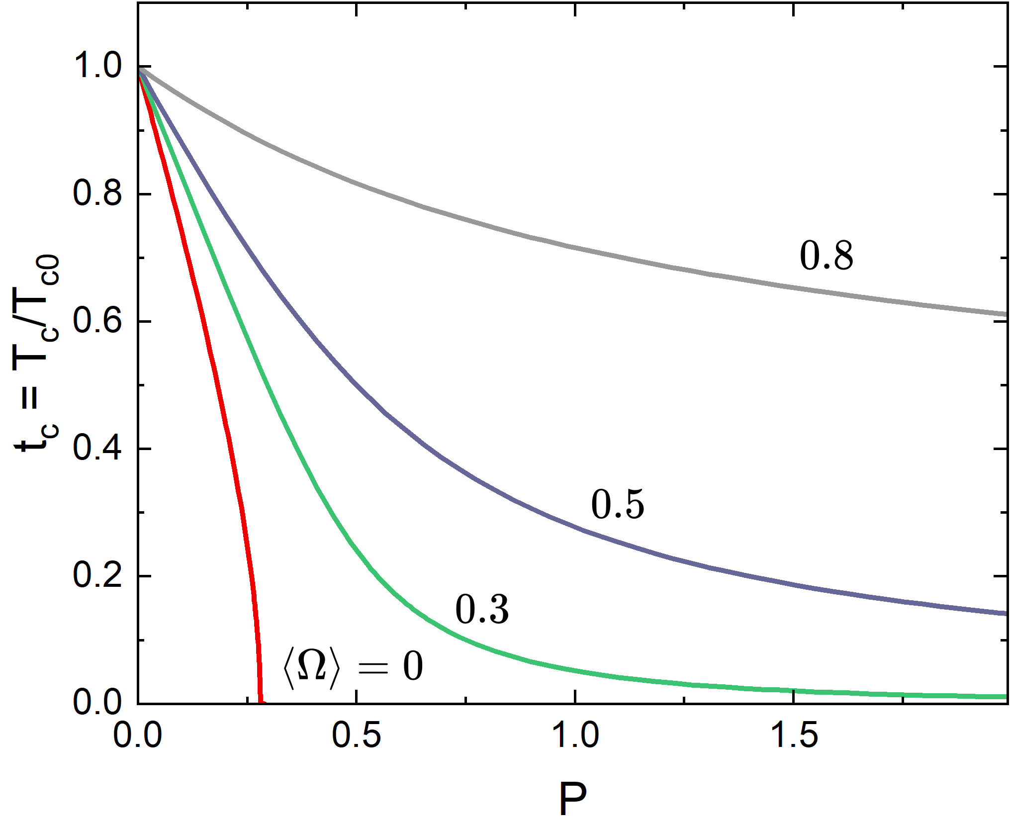
Figure 1: (Color online) $t_{c}=T_{c}/T_{c0}$ vs scattering parameter $P$ for $\langle\Omega\rangle=0.8,0.5,0.3,0$ in top-down order. Note that for d-wave $\langle\Omega\rangle=0$ and $T_{c}$ turns zero at the critical scattering $P_{crit}=1/2e^{\gamma}=0.2807$.

Clearly, $T_{c}=T_{c0}$ for the isotropic order parameter with $\Omega=1$ and arbitrary scattering rate $P$ as well as for the clean limit and any anisotropic $\Omega$. For the d-wave $\langle\Omega\rangle=0$ and we have the standard Abrikosov-Gor’kov result [15] so that the transport scattering in d-wave affects $T_{c}$ as the pair-breaking scattering in isotropic materials does.

II Linearized Ginzburg-Landau equations

Thus, according to Eq. (3), the slope of $H_{c2}$ at $T_{c}$ is determined by the coherence length which enters linearized GL equation for the order parameter $\Psi$,

$$-(\xi^{2})_{ik}\Pi_{i}\Pi_{k}\Psi=\Psi$$ (8)

with the tensor of squared coherence length $(\xi^{2})_{ik}$; ${\bm{\Pi}}=\nabla+2\pi i{\bm{A}}/\phi_{0}$, $\bm{A}$ is the vector potential and $\phi_{0}$ is the flux quantum. For arbitrary $\Omega$ and any Fermi surface in presence of transport scattering, A. Pokrovsky and V. Pokrovsky [8] evaluated the tensor

$$(\xi^{2})_{ik}=\zeta_{ik}/a\,.$$ (9)

Here, (in our notation)

$$a=\frac{T_{c}-T}{T_{c}}\left[1+(1-\langle\Omega\rangle^{2})\psi^{\prime}\left(\frac{P/t_{c}+1}{2}\right)\right]\,.$$ (10)

The tensor $\hat{\zeta}$ is given by

$$\zeta_{ik} = \frac{\hbar^{2}}{16\pi^{2}T_{c}^{2}}\Big{[}h_{3,0}\langle\Omega^{2}v_{i}v_{k}\rangle$$ (11)

$$+ \frac{P}{t_{c}}h_{3,1}\langle\Omega v_{i}v_{k}\rangle\langle\Omega\rangle+\frac{P^{2}}{4t_{c}^{2}}h_{3,2}\langle v_{i}v_{k}\rangle\langle\Omega\rangle^{2}\Big{]}\,.$$

The quantities $h_{\mu,\nu}$ are functions of $x=P/2t_{c}$ defined as

$$h_{\mu,\nu}(x)=\sum_{n=0}^{\infty}(n+1/2+x)^{-\mu}(n+1/2)^{-\nu}\,,$$ (12)

so that

$$h_{3,0} = -\frac{1}{2}\psi^{\prime\prime}\left(\frac{1}{2}+x\right)\,,$$

$$h_{3,1} = \frac{1}{x^{3}}\Big{[}\psi\left(\frac{1}{2}+x\right)-\psi\left(\frac{1}{2}\right)-x\psi^{\prime}\left(\frac{1}{2}+x\right)$$

$$+ \frac{x^{2}}{2}\psi^{\prime\prime}\left(\frac{1}{2}+x\right)\Big{]}\,,$$

$$h_{3,2} = \frac{1}{2x^{4}}\Big{\{}\pi^{2}x-6\left[\psi\left(\frac{1}{2}+x\right)-\psi\left(\frac{1}{2}\right)\right]$$ (13)

$$+ 4x\psi^{\prime}\left(\frac{1}{2}+x\right)-x^{2}\psi^{\prime\prime}\left(\frac{1}{2}+x\right)\Big{\}}.$$

It is straightforward to see that for the isotropic order parameter with $\Omega=1$ on the Fermi sphere these formulas reduce to the BCS form

$$\xi^{2}=\frac{7\zeta(3)}{48\pi^{2}T_{c}^{2}\delta t}\chi(P)\,,\quad\delta t=1-\frac{T}{T_{c}}\,,$$ (14)

with the Gor’kov function

$$\chi(P)=\frac{1}{7\zeta(3)}\sum_{n=0}^{\infty}\frac{1}{(n+1/2+P)(n+1/2)^{2}}\,.$$ (15)

This limit can also be checked by comparison with $H_{c2}$ slopes at $T_{c}$ given by Helfand and Werthamer [11].

It is worth noting that for the clean limit $x=P/2t_{c}\to 0$, and $h_{3,0}\to 7\zeta(3)$, $h_{3,1}\to\pi^{4}/6$, and $h_{3,2}\to 31\zeta(5)$. This means that in this limit, only the first term on RHS of Eq. (11) survives in agreement with [9]. In the opposite limit $x=P/2t_{c}\gg 1$, the last term in Eq. (11) dominates [8] as is seen in Fig. 2 (however, this limit does not apply for the d-wave since both the second and the third terms in Eq. (11) are zeroes due to $\langle\Omega\rangle=0$).

II.1 General order parameter

In he general case we obtain for the slope of $H_{c2}$ along the $c$ axis of a uniaxial material

$$\frac{\partial H_{c2}}{\partial T}\Big{|}_{T_{c}}=-\frac{8\pi\phi_{0}T_{c0}}{\hbar^{2}}\frac{t_{c}\left[1+(1-\langle\Omega\rangle^{2})\psi^{\prime}\left(\frac{1+P/t_{c}}{2}\right)\right]}{h_{3,0}\langle\Omega^{2}v_{a}^{2}\rangle+2(P/2t_{c})h_{3,1}\langle\Omega\rangle\langle\Omega v_{a}^{2}\rangle+(P/2t_{c})^{2}h_{3,2}\langle\Omega\rangle^{2}\langle v_{a}^{2}\rangle}\,.\qquad$$ (16)

Here, all coefficients $h_{\mu,\nu}(x)$ are taken at $x=P/2t_{c}$.

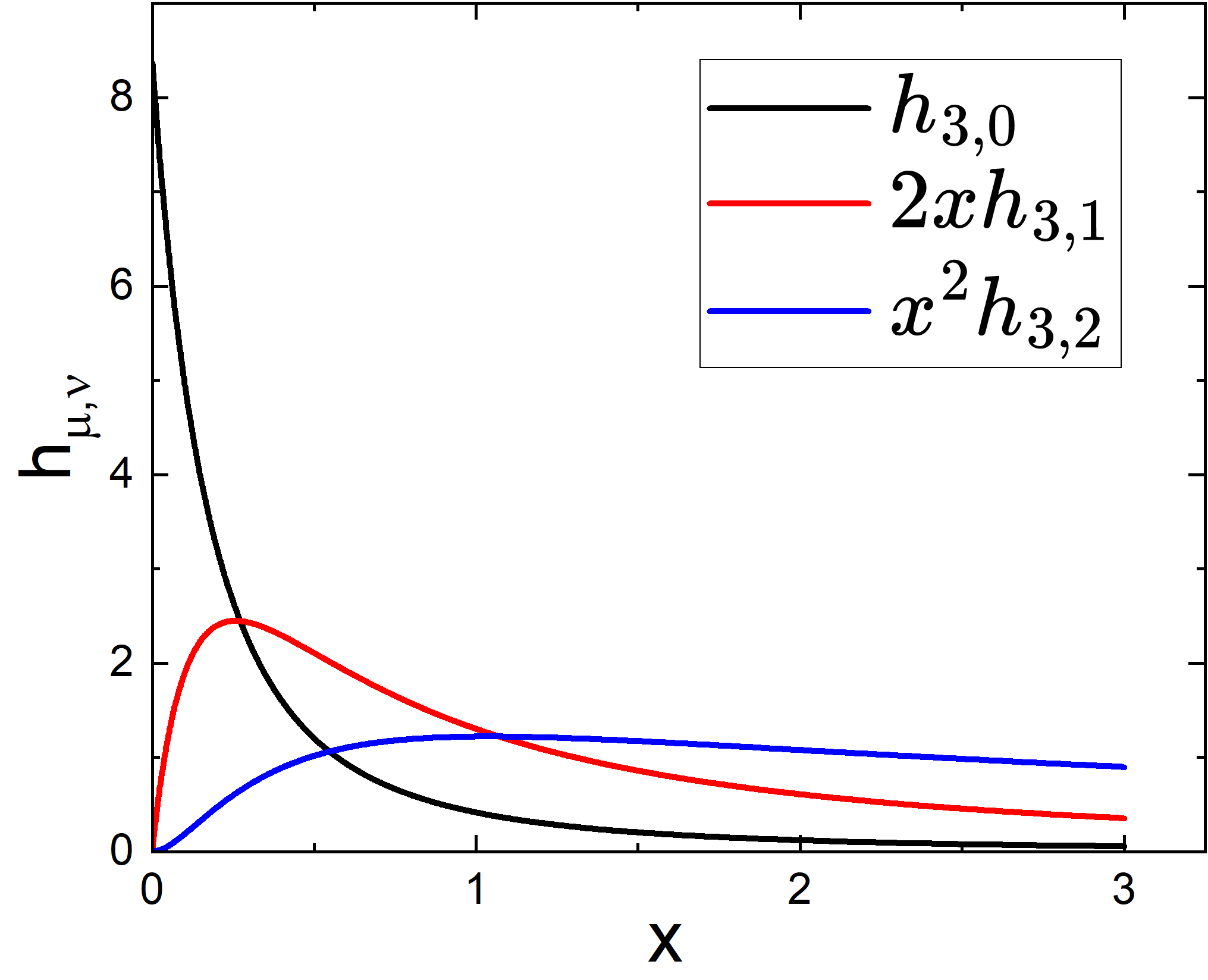
Figure 2: (Color online) The coefficients $h_{3,0}(x)$, $2xh_{3,1}(x)$, and $x^{2}h_{3,2}(x)$ vs $x$.

Since the Fermi velocity is not a constant at anisotropic Fermi surfaces, we normalize velocities on some value $v_{0}$ for which we choose [12]

$$v_{0}^{3}=2E_{F}^{2}/\pi^{2}\hbar^{3}N(0)\,,$$ (17)

where $E_{F}$ is the Fermi energy and $N(0)$ is the total density of states at the Fermi level per spin. One easily verifies that $v_{0}=v_{F}$ for the isotropic case.

The slope expression (16) remains the same except a changed pre-factor

$$-\frac{8\pi\phi_{0}T_{c0}}{\hbar^{2}}\to-\frac{8\pi\phi_{0}T_{c0}}{\hbar^{2}v_{0}^{2}}\,,$$ (18)

and the velocity $v_{a}$ is now dimensionless (although we leave for it the same notation).

II.2 d-wave

The case of the d-wave symmetry of the order parameter with $\langle\Omega\rangle=0$ is relatively simple. We have the coherence length relevant for $H_{c2}$ along $c$ axis of a uniaxial crystal:

$$\xi_{aa}^{2} = \frac{\zeta_{aa}}{a}=\frac{\hbar^{2}\langle\Omega^{2}v_{a}^{2}\rangle h_{3,0}}{16\pi^{2}T_{c}^{2}\left[1+\psi^{\prime}(P/2t_{c}+1/2)\right]\delta t}.$$ (19)

For a Fermi cylinder, with $\Omega=\sqrt{2}\cos 2\varphi$, the average $\langle\Omega^{2}v_{a}^{2}\rangle=v^{2}/2$. Hence,

$$\xi_{aa}^{2}=-\frac{\hbar^{2}v^{2}\,\psi^{\prime\prime}(P/2t_{c}+1/2)}{64\pi^{2}T_{c}^{2}\left[1+\psi^{\prime}(P/2t_{c}+1/2)\right]\delta t}.$$ (20)

and we obtain:

$$\frac{dH_{c2,c}}{dT}\Big{|}_{T_{c}}=\frac{32\pi\phi_{0}T_{c0}}{\hbar^{2}v^{2}}\,t_{c}\frac{1+\psi^{\prime}(P/2t_{c}+1/2)}{\psi^{\prime\prime}(P/2t_{c}+1/2)}.$$ (21)

For numerical work it is convenient to use the reduced slope

$$S=-\frac{dh_{c2}}{dt}\Big{|}_{t_{c}}=-\frac{\hbar^{2}v^{2}}{8\pi\phi_{0}T_{c}}\frac{dH_{c2}}{dT}\Big{|}_{T_{c}}\,.$$ (22)

While the actual slope $\left.\partial H_{c2}/\partial T\right|_{T_{c}}$ is negative, we are interested in its magnitude and use a positive quantity as given by Eq. (22).

The behavior of the slope as a function of $P$ according to this result is shown in Fig. 3. As is known, the maximum scattering parameter $P$ for which the d-wave superconductivity survives is $P_{{\rm{crit}}}=1/2e^{\gamma}=0.28$ (the double of the critical value for the spin-flip magnetic scattering [15]). Hence, similar to materials with magnetic scatterers [16], the slope $\partial H_{c2}/\partial T$ at $T_{c}$ for d-wave decreases with increasing transport scattering. It is worth noting that this behavior changes to increase near $P\approx 0.91\,P_{{\rm{crit}}}=0.25$; this estimate coincides with that given by Abrikosov and Gor’kov for the low bound of the gapless state. This suggests that d-wave materials can also be gapless if the transport scattering parameter lays in the interval $0.25<P<0.28$. Thus, $S(P)$ dependence might be a macroscopic manifestation of the gapless superconductivity in impure d-wave materials, the speculation worth of further study.

Figure 4 shows the slopes of Fig. 3 plotted vs the critical temperate $t_{c}(P)$.

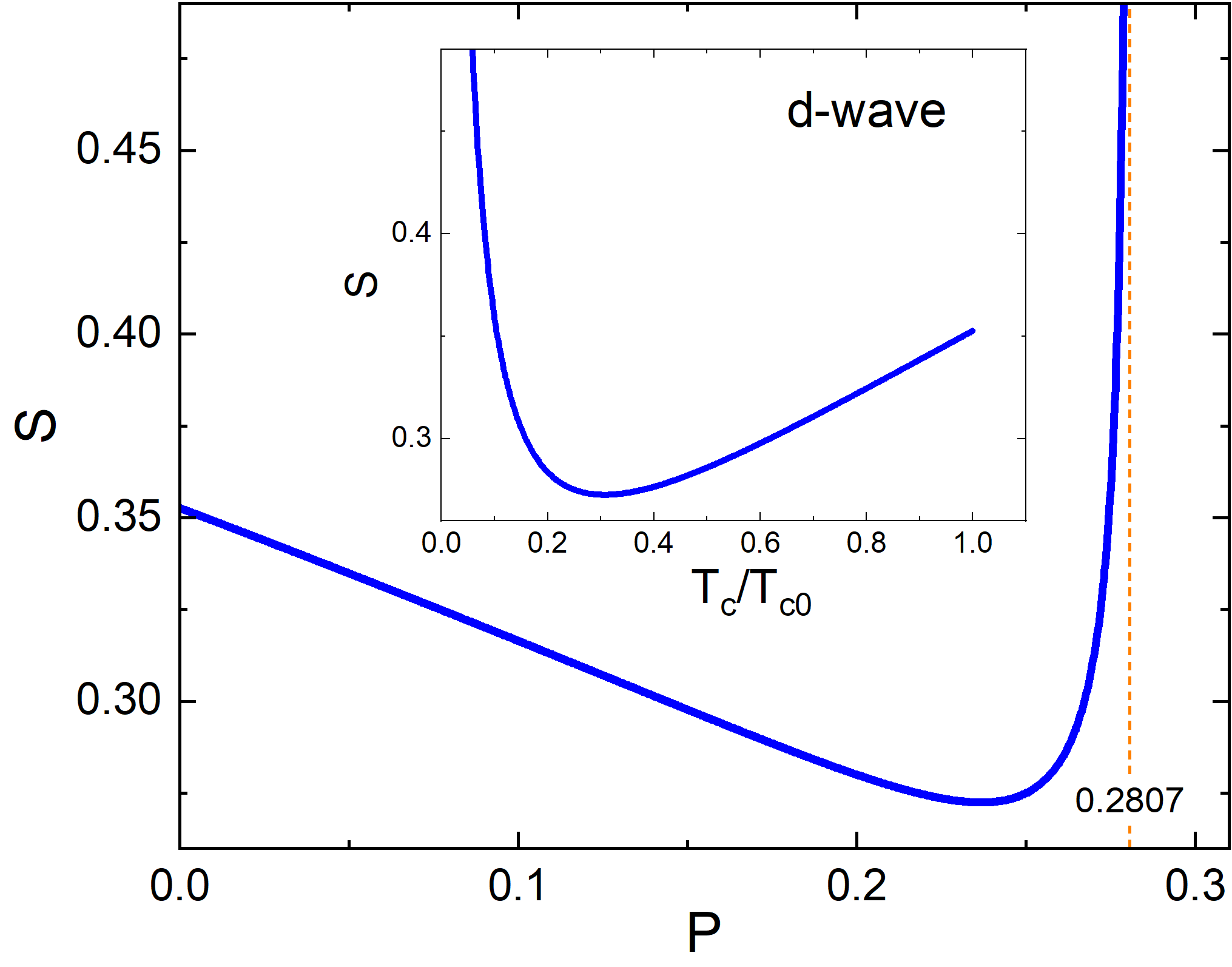
Figure 3: (Color online) The slope $S=\partial h_{c2}/\partial h$ at $t_{c}$ according to Eq. (22) vs $P$ for a d-wave material. Inset: the same slopes vs $t_{c}=T_{c}/T_{c0}$.

II.3 $\bm{s+d}$

Obviously the major interest in the community is to determine whether the easily accessible measurements of the $H_{c2}$ slope near $T_{c}$, may provide some insight into the structure of the order parameter. Here we examine the simplest case of a $s+d$ state where order parameter is the isotropic s-wave in one limit and a standard 2D $d-$wave in the other. Keeping in mind the normalization, $\langle\Omega^{2}\rangle=1,$ a convenient order parameter can be written as:

$$\Omega=\sqrt{1-r^{2}/2}+r\cos(2\varphi)$$ (23)

If $r=0$, $\Omega=1$ and when $r=\sqrt{2}$, $\Omega=\sqrt{2}\cos(2\varphi)$ which are the required limiting cases. We choose this order parameter not because it may describe any particular real material, rather we intend to check whether or not there is a connection between the microscopic anisotropy of the order parameter and the macroscopic dependence $S(P)$ of slopes of $H_{c2}$ on the degree of disorder $P$.

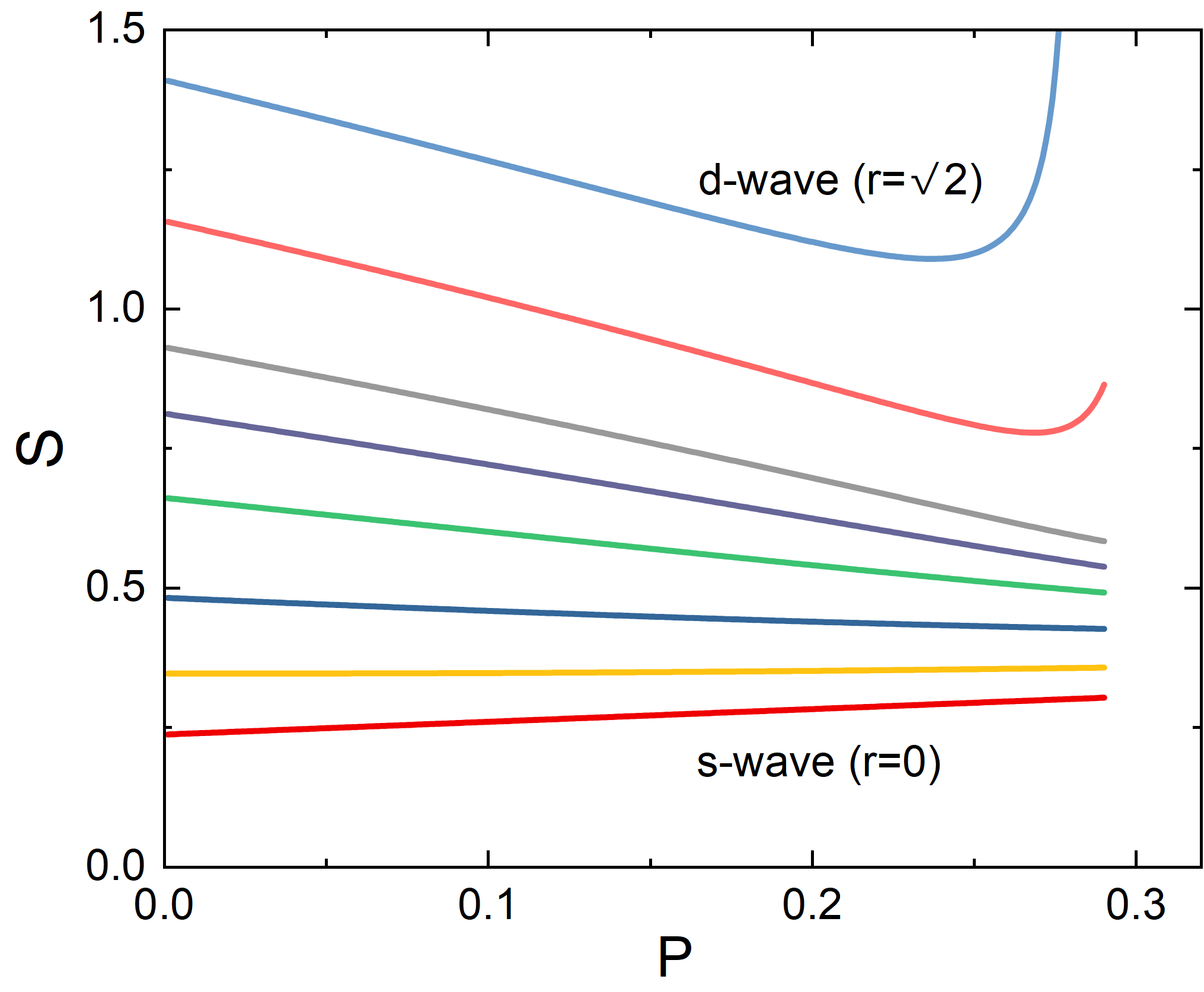
Figure 4: (Color online) $S(P)$ according to Eqs. (22) and (16) for a set of parameter $r=0,0.75,1,1.2,1.3,1.35,1.4$ and $\sqrt{2}$. The approach to a gapless regime is characterized by an upturn starting with $P\approx 0.25$ for a $d$-wave order parameter with $r=\sqrt{2}$. The calculations were performed for a cylindrical Fermi surface.

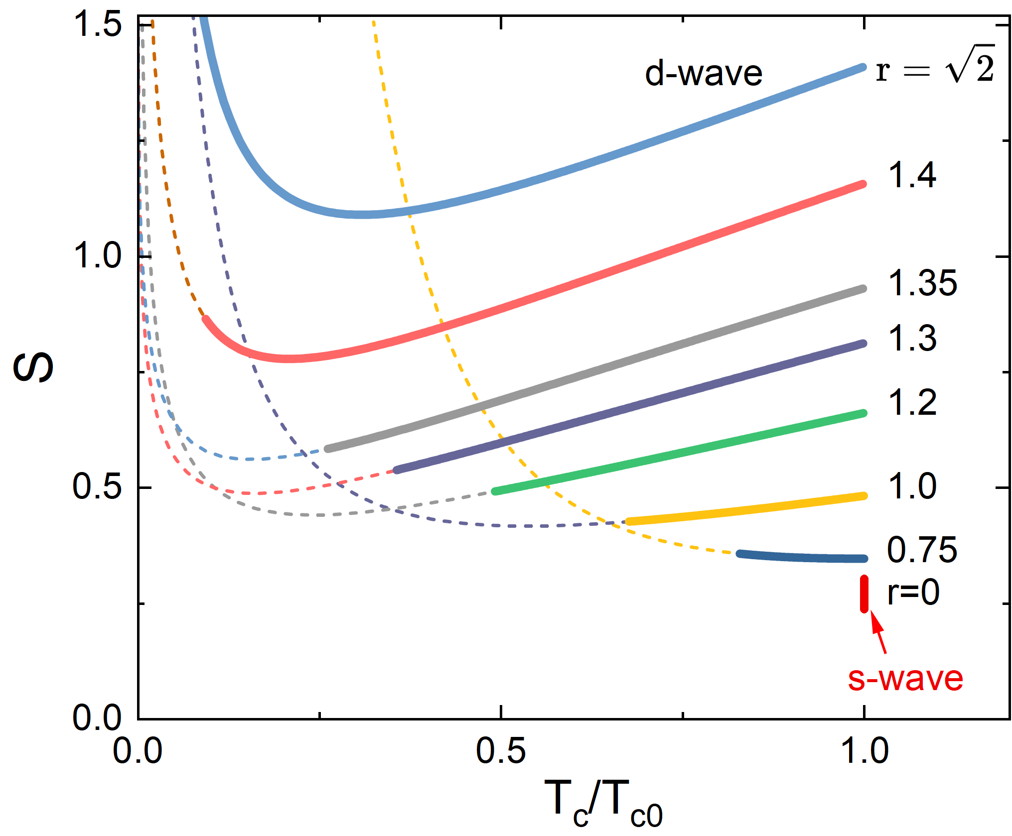
Figure 5: (Color online) Solid lines are the slopes $S$ for the same values of the scattering parameters $P$ as in Fig. 4, but plotted versus the transition temperature $t_{c}(P)$. Dashed continuations are for $P>0.28$ for which the pure d-wave phase does not exist. In the pure $s$-wave for which $t_{c}=1$, $S(P)$ does not depend on $P$ and shown by a vertical red line.

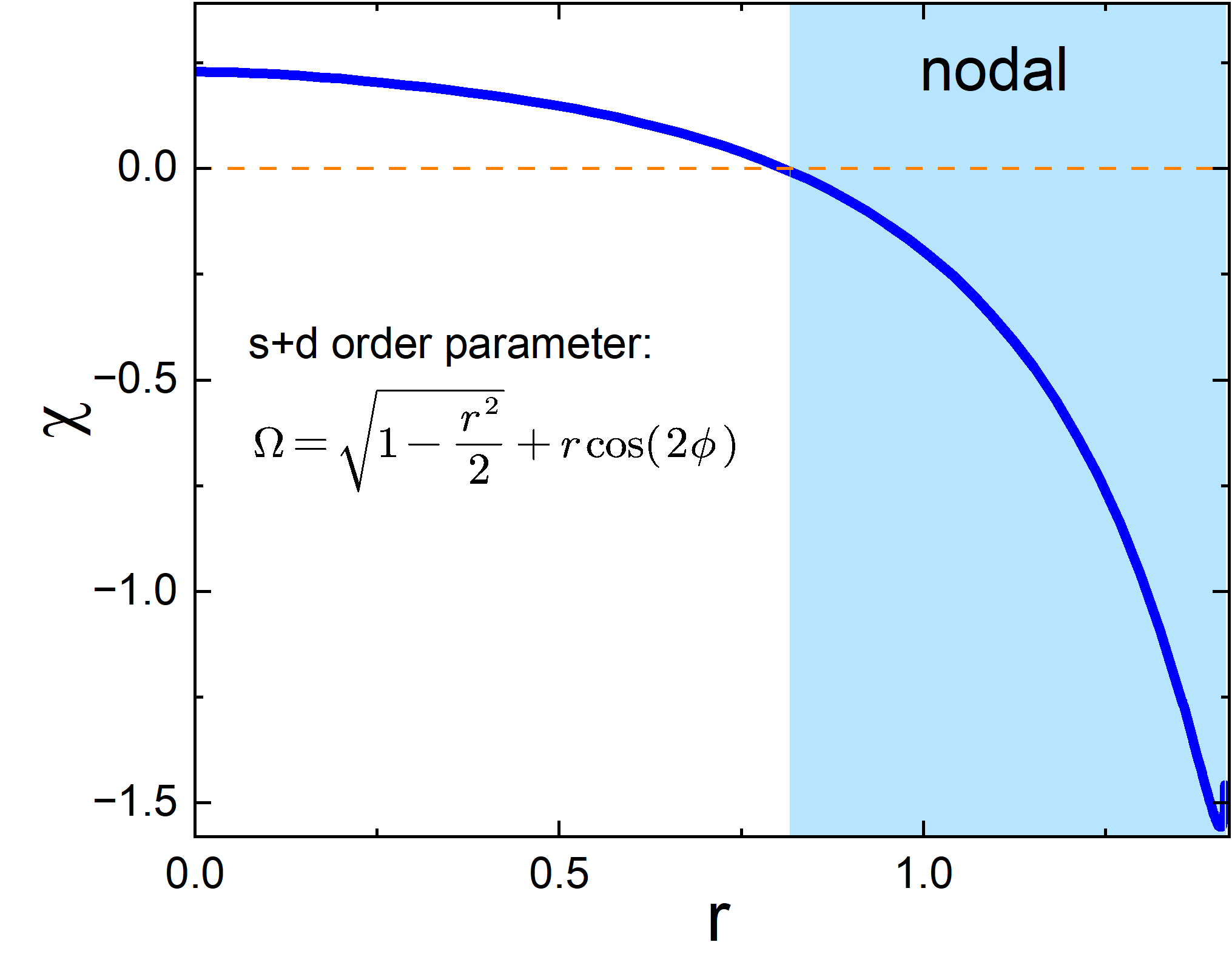
Figure 6: (Color online) The rate of change of the slope $S(P)$ defined as $\chi=S(0.11)-S(0.01))/0.1$, evaluated for different values of the $r$-coefficient. Nodal behavior starts at $r=\sqrt{2/3}\approx 0.817$. Apparently, this coincides with the rate of slope change becoming negative.

Figure 4 shows $S(P)$ calculated with the help of Eqs. (16), (22), plotted for a few coefficients $r$ of the $\Omega$ function, Eq. (23). At $r=0$ the order parameter is the isotropic $s$-wave, whereas at $r=\sqrt{2}$ it is a two-dimensional d-wave order parameter. The calculations were performed for a cylindrical Fermi surface keeping in mind possible applications of this work to high-$T_{c}$ cuprates. Figure 4 shows that the slopes $S(P)$ for purely d-wave are (a) non-monotonic and decrease with increasing $P$ up to about $P=0.25$ following by divergence when $P\to 0.28$, as we have seen in Fig. 3. With increasing fraction of s-wave, however, the negative slope of $S(P)$ for small and intermediate $P$ weakens and turns to positive nearly linear increase of $S$. To gain a further insight, we plot $S(P)$ versus $t_{c}$ in Fig. 5.

Since the overall behavior of the slopes $S(P)$ depends on fractions of $s$ and $d$ phases, we consider the relative difference $\chi=S(0.11)-S(0.01))/0.1$ which characterizes this behavior, i.e. increase for $\chi>0$ and decrease for $\chi<0$. Figure 6 shows this difference plotted versus coefficient $r$ of the order parameter, Eq. (23). A straightforward algebra shows that the order parameter is nodeless (anisotropic $s$) for $r<\sqrt{2/3}\approx 0.82$ and has four line nodes for $r>\sqrt{2/3}$. Remarkably, Fig. 6 shows that the rate of slope change $\chi$ becomes negative as soon as the nodes appear. In other words, if one would measure $\left|S\right|=|\partial H_{c2}/\partial T|_{T_{c}}|$ as a function of non-magnetic disorder, the increasing $S$ would indicate nodeless superconductivity, whereas the slope decrease can be considered as evidence for the nodes presence.

III Discussion

We have applied the GL theory developed by S. Pokrovsky and V. Pokrovsky [8] for anisotropic materials in the presence of non-magnetic scattering to evaluate slopes $\partial H_{c2}/\partial T|_{T_{c}}$ for d-wave superconductors and for the case of mixed $s+d$ symmetry. For the d-wave, we find that for weak and intermediate scattering rates $P=\hbar/2\pi T_{c0}\tau$, the slopes $S=-\partial H_{c2}/\partial T|_{T_{c}}$ are suppressed, similar to the situation of the magnetic pair-breaking disorder and opposite to the transport scattering enhancement of slopes $S(P)$ for the $s$-wave. One example of such a behavior is in studies of slopes in YBaCuO by Antonov et al. [17].

Unexpectedly however, if the scattering rate approaches the critical value $P_{crit}=0.28$ for which $T_{c}\to 0$, the slopes increase starting with $P\approx 0.25$ to diverge at $P_{crit}$. The value $0.25\approx 0.9$ of $P_{crit}$, the fraction found by Abrikosov and Gor’kov for the low bound of the gapless domain in standard $s$-wave materials with magnetic impurities [15]. This analogy suggests strongly that in d-wave with non-magnetic disorder close to the maximum disorder possible we are dealing with a kind of “gapless” state. In our view, this speculation deserves careful examination.

The slopes at $T_{c}$ are the easiest thing one can measure after a new superconductor is discovered. It has been done in-situ even for room-temperature materials under extremely high pressures within diamond pressure cells. If indeed, the easily done macroscopic measurement of slopes at $T_{c}$ may provide even partial information on the microscopic symmetry of the order parameter, this would be a worthy thing to do.

Thinking along these lines, we have examined the mixed $s+d$ order parameter $\Omega(r)=\sqrt{1-r^{2}/2}+r\cos(2\varphi)$ such that $\Omega(0)$ corresponds to the pure isotropic $s$-wave and $\Omega(\sqrt{2})$ is the pure $d$. We find the remarkable one-to-one correspondence between presence or absence of nodes and decrease or increase of the $H_{c2}$ slopes at $T_{c}$. Practically, this is a highly useful observation, notwithstanding our oversimplified model.

There are various ways to introduce point-like uniform disorder into superconductors. Perhaps the most promising and controllable are irradiation with neutrons or electrons, see e.g. [3] and [7]. To our knowledge, the slope $S$ in a nodal superconductor BaFe₂(As,P)₂ is decreasing up to large amounts of disorder [7].

Hence, one of our major results is a novel experimentally-simple way to distinguish between nodeless and nodal superconductivity. One has to examine the rate of change of the slopes in samples of the same chemical composition but with different amount of non-magnetic disorder. Such disorder can be induced by ion implantation [18, 17], electron [2], proton [19], neutron [3, 20], or gamma [21] and even alpha particle irradiation [22]. If it decreases, the system is likely nodal. If not, it is not.

A word of caution. It is quite possible that complex multi-band materials will not follow our simple scheme, employing the generally accepted factorization of temperature and angular variations of the order parameter. It is also possible that other types of order parameters, say triplet, will not follow either. However, our analysis is based on universal Ginzburg-Landau theory and, hopefully, our conclusions may turn out robust.

- [1] S. Tokuta and A. Yamamoto, Enhanced Upper Critical Field in Co-Doped Ba122 Superconductors by Lattice Defect Tuning, APL Mater. 7, 111107 (2019).
- [2] in preparation for submission. Experimental investigation of the slope in BaK122 of different compositions.
- [3] A. E. Karkin, T. Wolf, B. N. Goshchitskii, Superconducting properties of (Ba,K)Fe2As2 single crystals disordered with fast neutron irradiation. J. Phys.: Cond. Mat. 26, 275702 (2014), doi:10.1088/0953-8984/26/27/275702.
- [4] K. Hashimoto, K. Cho, T. Shibauchi, S. Kasahara, Y. Mizukami, R. Katsumata, Y. Tsuruhara, T. Terashima, H. Ikeda, M. A. Tanatar, H. Kitano, N. Salovich, R. W. Giannetta, P. Walmsley, A. Carrington, R. Prozorov, and Y. Matsuda, A Sharp Peak of the Zero-Temperature Penetration Depth at Optimal Composition in BaFe2(AsPx)2, Science (80) 336, 1554 (2012).
- [5] A. I. Posazhennikova and M. V. Sadovski, The Ginzburg-Landau expansion and the slope of the upper critical field in disordered superconductors, Pis’ma Zh. Eksp. Teor. Fiz. 63, 347 (1996).
- [6] A. I. Posazhennikova and M. V. Sadovski, The Ginzburg-Landau expansion and the slope of the upper critical field in superconductors with anisotropic normal-impurity scattering, Zh. Eksp. Teor. Fiz 112, 2124 (1997).
- [7] A significant suppression of and of the slope of the upper critical field was observed in line-nodal iron pnictide, BaFe2(As,P)2. [Private communication].
- [8] S. V. Pokrovsky, V. L. Pokrovsky,Density of states and order parameter in dirty anisotropic superconductors, Phys. Rev. B 54, 13275 (1996).
- [9] D. Markowitz and L. P. Kadanoff, Effect of Impurities upon Critical Temperature of Anisotropic Superconductors, Phys. Rev. 131, 563 (1963).
- [10] L. P. Gor’kov and T. K. Melik-Barkhudarov, Microscopic Derivation of the Ginzburg-Landau Equations for an Anisotropic Superconductor, Soviet Phys. JETP 18, 1031 (1964).
- [11] E. Helfand and N.R. Werthamer, Temperature and Purity Dependence of the Superconducting Critical Field, . II, Phys. Rev. 147, 288 (1966).
- [12] V. G. Kogan and R. Prozorov, Orbital Upper Critical Field and Its Anisotropy of Clean One- and Two-Band Superconductors, Rep. Prog. Phys. 75, 114502 (2012).
- [13] L. A. Openov, Combined effect of nonmagnetic and magnetic scatterers on the critical temperatures of superconductors with different anisotropies of the gap, JETP Lett. 66, 661 (1997).
- [14] V. G. Kogan, Pair breaking in iron pnictides, Phys. Rev. B 80, 214532 (2009).
- [15] A. A. Abrikosov and L. P. Gor’kov, Contribution to the theory of superconducting alloys with paramagnetic impurities, Zh. Eksp. Teor. Fiz. 39, 1781 (1060) [Sov. Phys. JETP 12, 1243 (1961)].
- [16] V. G. Kogan, R. Prozorov, Orbital upper critical field of type-II superconductors with pair breaking, Phys. Rev. B88, 024503 (2013).
- [17] A. Antonov V, A. Ikonnikov V, D. Masterov V, A. N. Mikhaylov, S. Morozov V, Y. N. Nozdrin, S. A. Pavlov, A. E. Parafin, D. Tetel’baum I, S. S. Ustavschikov, V. K. Vasiliev, P. A. Yunin, D. A. Savinov, Critical-field slope reduction and upward curvature of the phase-transition lines of thin disordered superconducting YBa2Cu3O7-x films in strong magnetic fields, Physica C - Superconductivity and its Applications 568 (2020), doi:10.1016/j.physc.2019.1353581.
- [18] R. H. T. Wilke, S. L. Bud’ko, P. C. Canfield, D. K. Finnemore, R. J. Suplinskas, S. T. Hannahs, Systematic Effects of Carbon Doping on the Superconducting Properties of MgB2. Phys. Rev. Lett. 92, 217003 (2004).
- [19] J. Kim, N. Haberkorn, M. J. Graf, I. Usov, F. Ronning, L. Civale, E. Nazaretski, G. F. Chen, W. Yu, J. D. Thompson, R. Movshovich, Magnetic penetration-depth measurements of a suppressed superfluid density of superconducting Ca0.5Na0.5Fe2As2 single crystals by proton irradiation. Phys. Rev. B 86, 144509 (2012), doi:10.1103/PhysRevB.86.144509.
- [20] R. H. T. Wilke, S. L. Bud’ko, P. C. Canfield, J. Farmer, S. T. Hannahs, Systematic study of the superconducting and normal-state properties of neutron-irradiated MgB2, Phys. Rev. B 73, 134512 (2006).
- [21] A. A. E.-S. El-Hamalawy, M. M. El-Zaidia, E. A. G. E. A. Ghali, The Effects of Gamma-Radiation on the High Tc superconductors ErBa2Cu3O7-d, Jap. J. Appl. Phys. 31, 3529 (1992).
- [22] C. Tarantini, K. Iida, N. Sumiya, M. Chihara, T. Hatano, H. Ikuta, R. K. Singh, N. Newman, D. C. Larbalestier, Effect of alpha-particle irradiation on a NdFeAs(O,F) thin film, Supercon. Sci. Tech. 31, 034002 (2018), doi:10.1088/1361-6668/aaa821.