Conditionally Strongly Log-Concave Generative Models

Abstract

There is a growing gap between the impressive results of deep image generative models and classical algorithms that offer theoretical guarantees. The former suffer from mode collapse or memorization issues, limiting their application to scientific data. The latter require restrictive assumptions such as log-concavity to escape the curse of dimensionality. We partially bridge this gap by introducing conditionally strongly log-concave (CSLC) models, which factorize the data distribution into a product of conditional probability distributions that are strongly log-concave. This factorization is obtained with orthogonal projectors adapted to the data distribution. It leads to efficient parameter estimation and sampling algorithms, with theoretical guarantees, although the data distribution is not globally log-concave. We show that several challenging multiscale processes are conditionally log-concave using wavelet packet orthogonal projectors. Numerical results are shown for physical fields such as the $\varphi^{4}$ model and weak lensing convergence maps with higher resolution than in previous works.

1 Introduction

Generative modeling requires the ability to estimate an accurate model of a probability distribution from a training dataset, as well as the ability to efficiently sample from this model. Any such procedure necessarily introduces errors, due to limited expressivity of the model class, learning errors of selecting the best model within that class, and sampling errors due to limited computational resources. For high-dimensional data, it is highly challenging to control all errors with polynomial-time algorithms. Overcoming the curse of dimensionality requires exploiting structural properties of the probability distribution. For instance, theoretical guarantees can be obtained with restrictive assumptions of log-concavity, or with low-dimensional parameterized models. In contrast, recent deep-learning-based approaches such as diffusion models (Ramesh et al., 2022; Saharia et al., 2022; Rombach et al., 2022) have obtained impressive results for distributions which do not satisfy these assumptions. Unfortunately, in such cases, theoretical guarantees are lacking, and diffusion models have been found to memorize their training data (Carlini et al., 2023; Somepalli et al., 2022), which is inappropriate for scientific applications. The disparity between these two approaches highlights the need for models which combine theoretical guarantees with sufficient expressive power. This paper contributes to this objective by defining the class of conditionally strongly log-concave distributions. We show that it is sufficiently rich to model the probability distributions of complex multiscale physical fields, and that such models can be sampled with fast algorithms with provable guarantees.

Sampling and learning guarantees.

While the theory for sampling log-concave distributions is well-developed (Chewi, 2023), simultaneous learning and sampling guarantees for general non-log-concave distributions are less common. Block et al. (2020) establish a fast mixing rate of multiscale Langevin dynamics under a manifold hypothesis. Koehler et al. (2022) studies the asymptotic efficiency of score-matching compared to maximum-likelihood estimation under a global log-Sobolev inequality, which is not quantitative beyond globally log-concave distributions. Chen et al. (2022b, a) establish polynomial sampling guarantees for a reverse score-based diffusion, given a sufficiently accurate estimate of the time-dependent score. Sriperumbudur et al. (2013); Sutherland et al. (2018); Domingo-Enrich et al. (2021) study density estimation with energy-based models under different infinite-dimensional parametrizations of the energy. They use various metrics including score-matching to establish statistical guarantees that avoid the curse of dimensionality, under strong smoothness or sparsity assumptions of the target distribution. Finally, Balasubramanian et al. (2022) derive sampling guarantees in Fisher divergence of Langevin Monte-Carlo beyond log-concave distributions. While these hold under a general class of target distribution, such Fisher guarantees are much weaker than Kullback-Leibler guarantees. Bridging this gap requires some structural assumptions on the distribution.

Multiscale generative models.

Images include structures at all scales, and several generative models have relied on decompositions with wavelet transforms (Yu et al., 2020; Gal et al., 2021). More recently, Marchand et al. (2022) established a connection between the renormalization group in physics and a conditional decomposition of the probability distribution of wavelet coefficients across scales. These models rely on maximum likelihood estimations with iterated Metropolis sampling, which leads to a high computational complexity. They have also been used with score matching (Guth et al., 2022; Kadkhodaie et al., 2023) in the context of score-based diffusion models (Song et al., 2021), which suffer from memorisation issues.

Conditionally strongly log-concave distributions.

We consider probability distributions whose Gibbs energy is dominated by quadratic interactions,

$$p(x)=\frac{1}{Z}e^{-E(x)}~{}~{}\text{with }E(x)=\frac{1}{2}x^{\mathrm{T}}Kx+V(x).$$

The matrix $K$ is positive symmetric and $V$ is a non-quadratic potential. If $V$ is non-convex, then $p$ is a priori not log-concave. However, the Hessian of $E$ may be dominated by the large eigenvalues of $K$, whose corresponding eigenvectors define directions in which $p$ is log-concave. For multiscale stationary distributions, $K$ is a convolution whose eigenvalues have a power-law growth at high frequencies. As a result, the conditional distribution of high frequencies given lower frequencies may be log-concave.

Section 2 introduces factorizations of probability distributions into products of conditional distributions with arbitrary hierarchical projectors. If the projectors are adapted to obtain strongly log-concave factors, we prove that maximum likelihood estimation can be replaced by score matching, which is computationally more efficient. The MALA sampling algorithm also has a fast convergence due to the conditional log-concavity. Section 3 describes a class of multiscale physical processes that admit conditionally strongly log-concave (CSLC) decompositions with wavelet packet projections. This class includes the $\varphi^{4}$ model studied in statistical physics. These results thus provide an approach to provably avoid the numerical instabilities at phase transitions observed in such models. We then show in Section 4 that wavelet packet CSLC decompositions provide accurate models of cosmological weak lensing images, synthesized as test data for the Euclid outer-space telescope mission (Laureijs et al., 2011).

The main contributions of the paper are:

• The definition of general CSLC models, which provide learning guarantees by score matching and sampling convergence bounds with MALA.

• CSLC models of multiscale physical fields using wavelet packet projectors. We show that $\varphi^{4}$ and weak lensing both satisfy the CSLC property, which leads to efficient and accurate generative modeling.

The code to reproduce our numerical experiments is available at https://github.com/Elempereur/WCRG.

2 Conditionally Strongly Log-Concave Models

Section 2.1 introduces conditionally strongly log-concave models, by factorizing the probability density into conditional probabilities. For these models, Sections 2.2 and 2.3 give upper bounds on learning errors with score matching algorithms, and Section 2.4 on sampling errors with a Metropolis-Adjusted Langevin Algorithm (MALA). Proofs of the mathematical results can be found in Appendix E.

2.1 Conditional Factorization and Log-Concavity

We introduce a probability factorization based on orthogonal projections on progressively smaller-dimensional spaces. The projections are adapted to define strongly log-concave conditional distributions.

Orthogonal factorization.

Let $x\in\mathbb{R}^{d}$. A probability distribution $p(x)$ can be decomposed into a product of autoregressive conditional probabilities

$$p(x)=p(x[1])\prod_{i=2}^{d}p(x[i]\,|\,x[1],\dots,x[i-1]).$$ (1)

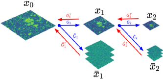
However, more general factorizations can be obtained by considering blocks of variables in an orthogonal basis. We initialize the decomposition with $x_{0}=x$. For $j=1$ to $J$, we recursively split $x_{j-1}$ in two orthogonal projections:

$$x_{j}=G_{j}x_{j-1}\text{ and }\bar{x}_{j}=\bar{G}_{j}x_{j-1},$$

where $G_{j}$ and $\bar{G}_{j}$ are unitary operators such that $G_{j}^{\mathrm{T}}G_{j}+\bar{G}_{j}^{\mathrm{T}}\bar{G}_{j}=\mathrm{Id}$. It follows that

$$x_{j-1}=G_{j}^{\mathrm{T}}x_{j}+\bar{G}_{j}^{\mathrm{T}}\bar{x}_{j}.$$ (2)

Let $d_{j}=\text{dim}(x_{j})$ and $\bar{d}_{j}=\text{dim}(\bar{x}_{j})$, then $d_{j-1}=d_{j}+\bar{d}_{j}$.

Since the decomposition is orthogonal, for any probability distribution $p$ we have

$$p(x_{j-1})=p(x_{j},\bar{x}_{j})=p(x_{j})p(\bar{x}_{j}|x_{j}).$$

Cascading this decomposition $J$ times gives

$$p(x)=p(x_{J})\prod_{j=1}^{J}p(\bar{x}_{j}|x_{j}),$$ (3)

which generalizes the autoregressive factorization (1). The properties of the factors $p(\bar{x}_{j}|x_{j})$ depend on the choice of the orthogonal projectors $G_{j}$ and $\bar{G}_{j}$, as we shall see below.

Model learning and sampling.

A parametric model $p_{\theta}(x)$ of $p(x)$ can be defined from Equation 3 by computing parametric models of $p(x_{J})$ and each $p(\bar{x}_{j}|x_{j})$:

$$p_{\theta}(x)=p_{\theta_{J}}(x_{J})\prod_{j=1}^{J}p_{\bar{\theta}_{j}}(\bar{x}_{j}|x_{j}),$$ (4)

with $\theta=(\theta_{J},\bar{\theta}_{j})_{j\geq J}$.

Learning this model then amounts to optimizing the parameters $\theta_{J},(\bar{\theta}_{j})_{j}$ from available data, so that the resulting distributions are close to the target. We measure the associated learning errors with the Kullback-Leibler divergences $\epsilon^{L}_{J}=\mathrm{KL}_{x_{J}}(p(x_{J})\,\|\,p_{\theta_{J}}(x_{J}))$ and

$$\bar{\epsilon}^{L}_{j}=\mathbb{E}_{x_{j}}\mathopen{}\mathclose{{}\left[\mathrm{KL}_{\bar{x}_{j}}(p(\bar{x}_{j}|x_{j})\,\|\,p_{\bar{\theta}_{j}}(\bar{x}_{j}|x_{j}))}\right],\ j\leq J.$$

Once the parameters have been estimated, we sample from $p_{\theta}$ as follows. We first compute a sample $x_{J}$ of $p_{\theta_{J}}$. The sampling introduces an error, which we measure with $\epsilon^{S}_{J}=\mathrm{KL}_{x_{J}}(\hat{p}_{\theta_{J}}(x_{J})\,\|\,p_{\theta_{J}}(x_{J}))$, where $\hat{p}_{\theta_{J}}$ is the law of the samples returned by the algorithm. For each $j\leq J$, given the sampled $x_{j}$, we compute a sample $\bar{x}_{j}$ of $p_{\bar{\theta}_{j}}(\bar{x}_{j}|x_{j})$ and recover $x_{j-1}$ with Equation 2, up to $j=1$, where it computes $x=x_{0}$. Let $\hat{p}_{\bar{\theta}_{j}}$ be the law of computed samples $\bar{x}_{j}$. It also introduces an error

$$\bar{\epsilon}^{S}_{j}=\mathbb{E}_{x_{j}}\mathopen{}\mathclose{{}\left[\mathrm{KL}_{\bar{x}_{j}}(\hat{p}_{\bar{\theta}_{j}}(\bar{x}_{j}|x_{j})\,\|\,p_{\bar{\theta}_{j}}(\bar{x}_{j}|x_{j}))}\right],\ j\leq J.$$

Let $\hat{p}$ be the (joint) law of the computed samples $x$. The following proposition relates the total variation distance $\mathrm{TV}(\hat{p},p)$ with the learning and sampling errors for each $j$.

Proposition 2.1 (Error decomposition).

$$\mathrm{TV}(\hat{p},p)\leq\frac{1}{\sqrt{2}}\mathopen{}\mathclose{{}\left(\sqrt{\epsilon^{L}_{J}+\sum_{j=1}^{J}\bar{\epsilon}^{L}_{j}}+\sqrt{\epsilon^{S}_{J}+\sum_{j=1}^{J}\bar{\epsilon}^{S}_{j}}}\right).$$

The overall error depends on the sum of learning and sampling errors for each conditional probability distribution. Therefore, to control the total error, we need sufficient conditions ensuring that each of these sources of error is small. We introduce CSLC models for this purpose.

Conditional strong log-concavity.

We recall that a distribution $p$ is strongly log-concave (SLC) if there exists $\beta[p]\geq\alpha[p]>0$ such that

$$\alpha[p]\mathrm{Id}\preceq-\nabla_{x}^{2}\log p(x)\preceq\beta[p]\mathrm{Id},\ \forall x.$$ (5)

Definition 2.1.

We say that $p(x)=p(x_{J})\prod_{j=1}^{J}p(\bar{x}_{j}|x_{j})$ is conditionally strongly log-concave (CSLC) if each $p(\bar{x}_{j}|x_{j})$ is strongly log-concave in $\bar{x}_{j}$ for all $x_{j}$.

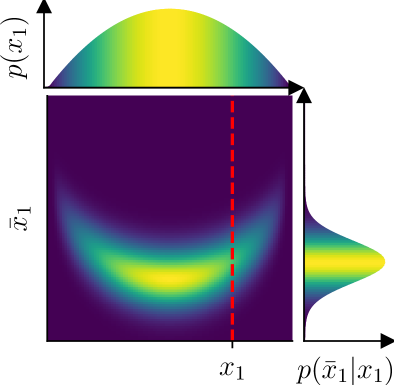
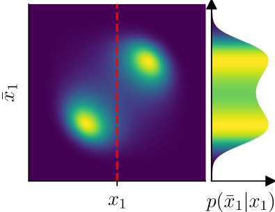
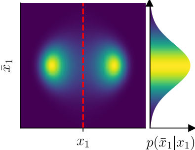
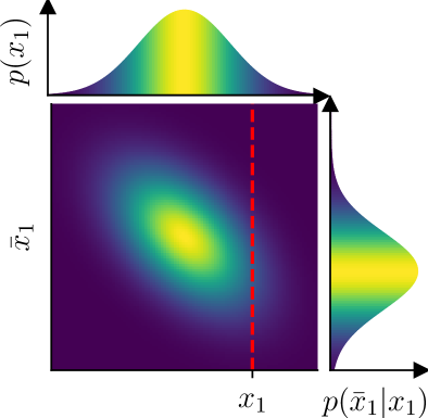
Conditional log-concavity is a weaker condition than (joint) log-concavity. If $p(x)$ is log-concave, then it has a convex support. On the other hand, conditional log-concavity only constraints slices (through conditioning) and projections (through marginalization) of the support of $p(x)$. Figure 1 illustrates that a jointly log-concave distribution is conditionally log-concave (and $p(x_{J})$ is furthermore log-concave), but the converse is not true. Conditional log-concavity also depends on the choice of the orthogonal projections $G_{j}$ and $\bar{G}_{j}$ which need to be adapted to the data. A major issue is to identify projectors that define a CSLC decomposition, if it exists. We show in Section 3 that this can be achieved for a class of physical fields with wavelet packet projectors.

Figure 1: A globally log-concave distribution is conditionally log-concave (top left), but the converse is not true (top right): a non-convex support can have convex vertical slices (and horizontal projection). Conditional log-concavity also depends on the choice of orthogonal projectors: a distribution can fail to be conditionally log-concave in the canonical basis (bottom left) but be conditionally log-concave after a rotation of $45$ degrees (bottom right).

The following subsections provide bounds on the learning and sampling errors $\bar{\epsilon}^{L}_{j}$ and $\bar{\epsilon}^{S}_{j}$ for CSLC models. To simplify notations, in the following we drop the index $j$ and replace $p_{\bar{\theta}_{j}}(\bar{x}_{j}|x_{j})$ with $p_{\bar{\theta}}(\bar{x}|x)$. We shall suppose that the dimension $d_{J}=\dim(x_{J})$ is sufficiently small so that $x_{J}$ can be modeled and generated with any standard algorithm with small errors $\epsilon^{L}_{J}$ and $\epsilon^{S}_{J}$ ($d_{J}=1$ in our numerical experiments).

2.2 Learning Guarantees with Score Matching

Fitting probabilistic models $p_{\bar{\theta}}(\bar{x}|x)$ by directly minimizing the $\mathrm{KL}$ errors $\bar{\epsilon}^{L}$ is computationally challenging because of intractable normalization constants. Strong log-concavity enables efficient yet accurate learning via a tight relaxation to score matching.

There exist several frameworks to fit a parametric probabilistic model to the data, most notably the maximum-likelihood estimator of a general energy-based model ${p}_{\bar{\theta}}(\bar{x}|x)=Z_{\bar{\theta}}^{-1}(x)e^{-\bar{E}_{\bar{\theta}}(x,\bar{x})}$, where $\bar{E}_{\bar{\theta}}$ is an arbitrary parametric class. This is computationally expensive due to the need to estimate the gradients of the normalization constants $-\nabla_{\bar{\theta}}\log Z_{\bar{\theta}}=\mathbb{E}_{{p}_{\bar{\theta}}}[\nabla_{\bar{\theta}}\bar{E}_{\bar{\theta}}]$ during training, which requires the ability to sample from $p_{\bar{\theta}}(\bar{x}|x)$. An appealing alternative which has enjoyed recent popularity is score matching (Hyvärinen & Dayan, 2005), which instead minimizes the Fisher Divergence $\mathrm{FI}$:

$$\ell(\bar{\theta}) =\mathbb{E}_{x}\mathopen{}\mathclose{{}\left[\frac{1}{2}\mathrm{FI}_{\bar{x}}({p}(\bar{x}|x)\,\|\,{p}_{\bar{\theta}}(\bar{x}|x))}\right]$$

$$=\mathbb{E}_{x,\bar{x}}\mathopen{}\mathclose{{}\left[\frac{1}{2}\|{-\nabla_{\bar{x}}\log p(\bar{x}|x)}-\nabla_{\bar{x}}\bar{E}_{\bar{\theta}}(x,\bar{x})\|^{2}}\right].$$

With a change of variables we obtain

$$\ell(\bar{\theta})=\mathbb{E}_{x,\bar{x}}\mathopen{}\mathclose{{}\left[\frac{1}{2}\|\nabla_{\bar{x}}\bar{E}_{\bar{\theta}}\|^{2}-\Delta_{\bar{x}}\bar{E}_{\bar{\theta}}}\right]+\mathrm{cst},$$ (6)

showing that $\ell({\bar{\theta}})$ can be minimized from available samples without estimating normalizing constants or sampling from $p_{\bar{\theta}}$. Indeed, given i.i.d. samples $\{(\bar{x}^{1},x^{1}),\dots,(\bar{x}^{n},x^{n})\}$ from $p(\bar{x},x)$, the empirical risk $\hat{\ell}(\bar{\theta})$ associated with score matching on $p(\bar{x}|x)$ is given by

$$\hbox{}\!\!\!\hat{\ell}({\bar{\theta}}) =\frac{1}{n}\sum_{i=1}^{n}\mathopen{}\mathclose{{}\left(\frac{1}{2}\|\nabla_{\bar{x}}\bar{E}_{\bar{\theta}}({x}^{i},\bar{x}^{i})\|^{2}-\Delta_{\bar{x}}\bar{E}_{\bar{\theta}}({x}^{i},\bar{x}^{i})}\right).$$ (7)

The score-matching objective avoids the computational barriers associated with normalization and sampling in high-dimensions, at the expense of defining a weaker metric than the KL divergence. This weakening of the metric is quantified by the log-Sobolev constant $\rho[p]$ associated with ${p}$. It is the largest $\rho>0$ such that $\mathrm{KL}(q\,\|\,{p})\leq\frac{1}{2\rho}\mathrm{FI}(q\,\|\,{p})$ for any $q$. Learning via score matching can therefore be seen as a relaxation of maximum-likelihood training, whose tightness is controlled by the log-Sobolev constant of the hypothesis class (Koehler et al., 2022). This constant can be exponentially small for general multimodal distributions, making this relaxation too weak. A crucial exception, however, is given by SLC distributions (or small perturbations of them), as shown by the Bakry-Emery criterion (Bakry et al., 2014, Definition 1.16.1): if $\alpha[p_{{{\bar{\theta}}}}(\bar{x}|x)]\geq\bar{\alpha}>0$ for all $x$, or equivalently if $\nabla^{2}_{\bar{x}}\bar{E}_{\bar{\theta}}\succeq\bar{\alpha}\mathrm{Id}$ for all $x,\bar{x}$, then $\rho[p_{{{\bar{\theta}}}}(\bar{x}|x)]\geq\bar{\alpha}$ for all $x$, and therefore

$$\bar{\epsilon}^{L}\leq\frac{1}{\bar{\alpha}}\ell(\bar{\theta}).$$ (8)

We remark that while Equation 8 does not make explicit CSLC assumptions on the reference distribution $p$, a consistent learning model implies that the conditional distribution $p(\bar{x}|x)$ is arbitrarily well approximated (in $\mathrm{KL}$ divergence) with SLC distributions—thus justifying the structural CSLC assumption on the target.

2.3 Score Matching with Exponential Families

In numerical applications, one cannot minimize the true score-matching loss $\ell$ as only a finite amount of data is available. We now show that a similar control as Equation 8 can be obtained for the empirical loss minimizer, whenever prior information enables us to define low-dimensional exponential models for $p_{\bar{\theta}}(\bar{x}|x)$ with good accuracy. It also provides a control on the critical parameter $\bar{\alpha}$, addressing the optimization and statistical errors.

We consider a linear model $\bar{E}_{\bar{\theta}}(x,\bar{x})={\bar{\theta}}^{\mathrm{T}}\bar{\Phi}(x,\bar{x})$ with a fixed potential vector $\bar{\Phi}(x,\bar{x})\in\mathbb{R}^{m}$ ($m$ is thus the number of parameters), and the corresponding minimization of the (conditional) score matching objective in Equation 7. Thanks to this linear parameterization, it becomes a convex quadratic form $\hat{\ell}({\bar{\theta}})=\frac{1}{2}{\bar{\theta}}^{\mathrm{T}}\hat{H}{\bar{\theta}}-{\bar{\theta}}^{\mathrm{T}}\hat{g}$, with

$$\hat{H} =\frac{1}{n}\sum_{i=1}^{n}{\nabla_{\bar{x}}\bar{\Phi}(x^{i},\bar{x}^{i})\nabla_{\bar{x}}\bar{\Phi}(x^{i},\bar{x}^{i})^{\mathrm{T}}}\in{\mathbb{R}}^{m\times m},$$

$$\hat{g} =\frac{1}{n}\sum_{i=1}^{n}{\Delta_{\bar{x}}\bar{\Phi}(x^{i},\bar{x}^{i})}\in{\mathbb{R}}^{m}.$$

It can be minimized in closed-form by inverting the Hessian matrix: ${\hat{\bar{\theta}}}=\hat{H}^{-1}\hat{g}$. As discussed, the sampling and learning guarantees of the model critically rely on the CSLC property, which is ensured as long as ${\hat{\bar{\theta}}}\in\Theta_{\bar{\alpha}}:=\{{\bar{\theta}}\,|\,\nabla_{\bar{x}}^{2}\bar{E}_{\bar{\theta}}(x,\bar{x})\succeq\bar{\alpha}\mathrm{Id},\ \forall\,(x,\bar{x})\}$ with $\bar{\alpha}>0$.

The following theorem leverages the finite-dimensional linear structure of the score-matching problem to establish fast non-asymptotic rates of convergence, controlling the excess risk in $\mathrm{KL}$ divergence.

Theorem 2.1 (Excess risk for CSLC exponential models).

Let ${\bar{\theta}}^{\star}=\arg\min\ell({\bar{\theta}})$ and $\hat{\bar{\theta}}=\arg\min\hat{\ell}(\bar{\theta})$. Assume:

1. $\bar{\theta}^{\star}\in\Theta_{\bar{\alpha}}$ for some $\bar{\alpha}>0$,

2. ${H}=\mathbb{E}\mathopen{}\mathclose{{}\left[\nabla_{\bar{x}}\bar{\Phi}\nabla_{\bar{x}}\bar{\Phi}^{\mathrm{T}}}\right]\succeq\eta\mathrm{Id}$ with $\eta>0$,

3. the sufficient statistics $\bar{\Phi}$ satisfy moment conditions E.2, regularity conditions E.3, and $\nabla\bar{\Phi}_{k}(x,\bar{x})$ is $M_{\bar{\Phi}}$-Lipschitz for any $k\leq m$ and all $x$ (see Appendix E).

Then when $n>m$, the empirical risk minimizer $\hat{\bar{\theta}}$ satisfies

$$\hat{\bar{\theta}}\in\Theta_{\hat{\bar{\alpha}}}\ \text{with }\mathbb{E}_{(\bar{x}^{i},x^{i})}\mathopen{}\mathclose{{}\left[\hat{\bar{\alpha}}}\right]\geq\bar{\alpha}-O\mathopen{}\mathclose{{}\left(\eta^{-1}\sqrt{\frac{m}{n}}}\right),$$ (9)

and, for $t\ll\sqrt{m}\ell(\bar{\theta}^{\star})$,

$$\bar{\epsilon}^{L}\leq\frac{\ell({\bar{\theta}}^{\star})}{\bar{\alpha}}(1+t)$$ (10)

with probability greater than $1-\exp\mathopen{}\mathclose{{}\left\{-O(n\log(tn/\sqrt{m}))}\right\}$ over the draw of the training data. The constants in $O(\cdot)$ only depend on moment and regularity properties of $\bar{\Phi}$.

The theorem provides learning guarantees for the empirical risk minimizer $\hat{\bar{\theta}}$ (compare Equations 8 and 10), and hinges on three key properties: the ability of the exponential family to approximate the true conditionals at each block (i) with small Fisher approximation error $\ell({\bar{\theta}}^{\star})$, (ii) with a sufficiently large strong log-concavity parameter $\bar{\alpha}$, and (iii) with a well-conditioned kernel $H$. In numerical applications, the number of parameters $m$ should be small enough to control the learning error for finite number of samples $n$, and to be able to compute and invert the Hessian matrix $\hat{H}$. We will define in Section 3 low-dimensional models that can approximate a wide range of multiscale physical fields.

The proof uses concentration of the empirical covariance $\hat{H}$, and combines both upper and lower tail probability bounds (Mourtada, 2022; Vershynin, 2012) to bound the expectation, similarly as known results for least-squares (Mourtada, 2022; Hsu et al., 2012). The statistical properties of score matching under exponential families have been studied in the infinite-dimensional setting by Sriperumbudur et al. (2013); Sutherland et al. (2018), where kernel ridge estimators achieve non-parametric rates $n^{-s}$, $s<1$. Compared to these, as an intermediate result, we achieve the optimal rate in $\mathrm{FI}$ divergence in $n^{-1}$ directly with the ridgeless estimator (Equation 36). The key assumption is (i), namely that the optimal model in the exponential family is SLC. Since our structural assumption on the target $p$ is precisely that its conditionals are SLC, it is reasonable to expect this to be generally true. For instance, this is the case if the model is well specified ($p=p_{\bar{\theta}^{\star}}$).

2.4 Sampling Guarantees with MALA

We illustrate the efficient sampling properties of CSLC distributions by focusing on a reference sampler given by the Metropolis-Adjusted Langevin Algorithm (MALA) with algorithmic warm-start, which enjoys well-understood convergence properties in this case:

Proposition 2.2 (MALA Sampling, Altschuler & Chewi (2023, Theorem 5.1)).

Suppose that $\bar{\alpha}\mathrm{Id}\preceq\nabla^{2}_{\bar{x}}\bar{E}_{\bar{\theta}}(\bar{x}|x)\preceq\bar{\beta}\mathrm{Id}$ for all $\bar{x},x$, and let $\bar{d}=\mathrm{dim}(\bar{x})$. Then $N$ steps of MALA produce a sample $\bar{x}$ with conditional law $\hat{p}_{\bar{\theta}}(\bar{x}|x)$ satisfying

$$\bar{\epsilon}^{S}\leq\exp\mathopen{}\mathclose{{}\left(-O\mathopen{}\mathclose{{}\left(\sqrt{\frac{N}{\sqrt{\bar{d}}\bar{\beta}/\bar{\alpha}}}}\right)}\right).$$

MALA can thus be used to sample from CSLC distributions with an exponential convergence, whose mixing time $\widetilde{O}(\sqrt{\bar{d}}\bar{\beta}/\bar{\alpha})$ is sublinear in the dimension $\bar{d}$ and linear in the condition number $\bar{\beta}/\bar{\alpha}$ of the Hessian $\nabla^{2}_{\bar{x}}\bar{E}_{\bar{\theta}}$. We also note that similar guarantees will hold for other high-precision Metropolis-Hastings samplers, such as Hamilton Monte-Carlo. Together, Propositions 2.1 and 2.2 and Theorem 2.1 imply a control on the total accumulated error for CSLC exponential models.

3 Wavelet Packet Conditional Log-Concavity

The CSLC property depends on the choice of the projectors $(\bar{G}_{j},G_{j})$ which need to be adapted to the data. We show that for a class of stationary multiscale physical processes, CSLC models can be obtained with wavelet packet projectors. These models exploit the dominating quadratic interactions at high frequencies by splitting the frequency domain in sufficiently narrow bands. It reveals a powerful mathematical structure in this class of complex distributions.

3.1 Energies with Scalar Potentials

In the following, $x\in{\mathbb{R}}^{d}$ is a $\sqrt{d}\times\sqrt{d}$ image or two-dimensional field. We denote $x[i]$ the value of $x$ at pixel or location $i$. An important class of stationary probability distributions $p(x)=Z^{-1}e^{-E(x)}$ are defined in physics from an energy composed of a two-point interaction term $K$ plus a potential that is a sum of scalar potentials $v$:

$$E(x)=\frac{1}{2}x^{\mathrm{T}}Kx+\sum_{i}v(x[i]).$$ (11)

The matrix $K$ is a positive symmetric convolution operator. Equation 11 generalizes both zero-mean Gaussian processes (if $v=0$ then $K$ is the inverse covariance) and distributions with i.i.d. components (if $K=0$ then $v$ is the negative log-density of the pixel values). The energy Hessian is given by

$$\nabla^{2}_{x}E(x)=K+\operatorname{diag}\mathopen{}\mathclose{{}\left(v^{\prime\prime}(x[i])}\right)_{i}.$$ (12)

If $v^{\prime\prime}(t)<0$ for some $t\in{\mathbb{R}}$ then we may get negative eigenvalues for some $x$, in which case the energy is not convex.

Equation 11 provides models of a wide class of physical phenomena (Marchand et al., 2022), including ferromagnetism. An important example is the $\varphi^{4}$ energy in physics, which is a non-convex energy allowing to study phase transitions and explain the nature of numerical instabilities (Zinn-Justin, 2021). It has a kinetic energy term defined by $K=-\beta\Delta$ where $\Delta$ is a discrete Laplacian that enforces spatial regularity, and its scalar potential is $v(t)=t^{4}-(1+2\beta)t^{2}$. It has a double-well shape which pushes the values of each $x[i]$ towards $+1$ and $-1$, and is thus non-convex. $\beta$ is an inverse temperature parameter. In the thermodynamic limit $d\to\infty$ of infinite system size, the $\varphi^{4}$ energy has a phase transition at $\beta_{c}\approx 0.68$ (Kaupužs et al., 2016). At small temperature ($\beta\geq\beta_{c}$), the local interactions in the energy give rise to long-range dependencies. Gibbs sampling then “critically slows down” (Podgornik, 1996; Sethna, 2021) due to these long-range dependencies.

Fast sampling can nevertheless be obtained by exploiting conditional strong log-concavity. Assume that there exists $\gamma>0$ such that $v^{\prime\prime}(t)\geq-\gamma$ for all $t\in{\mathbb{R}}$. It then follows that $\nabla^{2}_{x}E\succeq K-\gamma\mathrm{Id}$. We can thus obtain a convex energy by restricting $K$ over a subspace where its eigenvalues are larger than $\gamma$. The convolution $K$ is diagonalized by the Fourier transform, with positive eigenvalues that we write $\hat{K}(\omega)$ at all frequencies $\omega$. The value $\hat{K}(\omega)$ typically increases when the frequency modulus $|\omega|$ increases. A convex energy is then obtained with a projector over a space of high-frequency images, as shown in the following proposition.

Proposition 3.1 (Conditional log-concavity of scalar potential energies).

Consider the energy defined in Equation 11 and assume that $-\gamma\leq v^{\prime\prime}\leq\delta$ for some $\gamma,\delta>0$ and that $\hat{K}(\omega)=\lambda|\omega|^{\eta}$ for some $\eta>0$. Let $\bar{G}_{1}$ be an orthogonal projector over a space of signals whose Fourier transform have a support included over frequencies $\omega$ such that $|\omega|\geq|\omega_{0}|$ with $|\omega_{0}|>(\gamma/\lambda)^{1/\eta}$. Then the conditional probability $p(\bar{x}_{1}|x_{1})$ is strongly log-concave for all $x_{1}$.

The proof is in Appendix F and relies on a direct calculation of the Hessian of the conditional energy. This proposition proves that we obtain a strongly log-concave conditional distribution $p(\bar{x}_{1}|x_{1})$ with a sufficiently high-frequency filter $\bar{G}_{1}$. It is illustrated in the bottom row of Figure 1 on a simplified two-dimensional example inspired from the $\varphi^{4}$ energy. The distribution has two modes $x=(1,1)$ and $x=(-1,-1)$, and the Fourier coefficients are computed with a $45$ degrees rotation: $x_{1}=(x[1]+x[2])/\sqrt{2}$ and $\bar{x}_{1}=(x[2]-x[1])/\sqrt{2}$, which leads to a log-concave conditional distribution.

Multiscale physical fields with scalar potential energies (11) are often self-similar over scales, in the sense that lower-frequency fields $x_{j}$ can also be described with an energy in the form of Equation 11, with different parameters (Wilson, 1971). This explains why Proposition 3.1 can be iterated to obtain a CSLC decomposition. For $\varphi^{4}$ energies, the range of $\bar{G}_{1}$ is non-empty as soon as $\beta\geq\frac{1}{2}$, which includes the critical temperature $\beta_{c}\approx 0.68$ (though $\delta=\infty$). At the critical temperature, $x_{1}$ is further described by the same parameters $K$ and $v$ as $x$, so that a complete CSLC decomposition is obtained by iteratively selecting projectors $\bar{G}_{j}$ which isolate the highest frequencies of $x_{j-1}$.

Proposition 3.1 can be extended to general energies

$$E(x)=\frac{1}{2}x^{\mathrm{T}}Kx+V(x),$$

by assuming that the Hessian $\nabla^{2}V(x)$ is bounded above and below. Conditional log-concavity may then be found by exploiting dominating quadratic energy terms with a PCA of $K$. We believe that this general principle may hold beyond the case of scalar potential energies (11) considered here.

3.2 Wavelet Packets and Renormalization Group

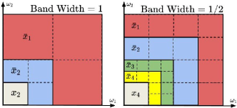
We now define wavelet packet projectors $G_{j}$ and $\bar{G}_{j}$, which are orthogonal projectors on localized zones of the Fourier plane. They are computed by convolutions with conjugate mirror filters and subsamplings (Coifman et al., 1992), described in Appendix A. These filters perform a recursive split of the frequency plane illustrated in Figure 2.

The wavelet packet $\bar{G}_{j}$ is a projector on a high-frequency domain, whereas $G_{j}$ is a projection on the remaining lower-frequency domain. An orthogonal wavelet transform is a particular example, which decomposes the Fourier plane into annuli of about one octave bandwidth, as shown in the top left and bottom panels of Figure 2. However, it may not be sufficiently well localized in the Fourier domain to obtain strictly convex energies. The frequency localization is improved by refining this split, as illustrated on the top right panel of Figure 2. Each $\bar{G}_{j}$ then performs a projection over a frequency annulus whose bandwidth is a half octave. Wavelet packets can adjust the frequency bandwidth to $2^{-{M+1}}$ octave for any integer $M\geq 1$. It allows reducing the support of $\bar{G}_{j}$, which is necessary to obtain a CSLC decomposition according to Proposition 3.1.

Figure 2: Top: frequency localization of the decomposition $(x_{J},\bar{x}_{J},\dots,\bar{x}_{1})$ with wavelet packet projectors of $1$ (left) and $1/2$ (right) octave bandwidths. Bottom: iterative decomposition of $x=x_{0}$ with $(\bar{G}_{j},G_{j})$ implementing a wavelet packet transformation over $J=2$ layers of $1$ octave bandwidth.

3.3 Multiscale Scalar Potentials

The probability distribution $p(x)$ is approximated by $p_{\theta}(x)=p_{\theta_{J}}(x_{J})\prod_{j=1}^{J}p_{\bar{\theta}_{j}}(\bar{x}_{j}|x_{j})$, where each $x_{j}$ and $\bar{x}_{j}$ are computed with wavelet packet projectors $G_{j}$ and $\bar{G}_{j}$. We introduce a parameterization of $p_{\bar{\theta}_{j}}$ with scalar potential energies, following Marchand et al. (2022). We shall suppose that the dimension $d_{J}=\mathrm{dim}(x_{J})$ is sufficiently small so that $p(x_{J})$ may be approximated with any standard algorithm ($d_{J}=1$ in our numerical experiments).

The self-similarity property of multiscale fields with scalar energies motivates the definition of each $p_{\bar{\theta}_{j}}(\bar{x}_{j}|x_{j})$ with an interaction energy

$$\bar{E}_{\bar{\theta}_{j}}(x_{j},\bar{x}_{j}) =\frac{1}{2}\bar{x}_{j}^{\mathrm{T}}\bar{K}_{j}\bar{x}_{j}+\bar{x}_{j}^{\mathrm{T}}\bar{K}^{\prime}_{j}x_{j}+\sum_{i}\bar{v}_{j}(x_{j-1}[i])$$

$$=\bar{\theta}_{j}^{T}\bar{\Phi}_{j}(x_{j},\bar{x}_{j}),$$ (13)

which derives from the fact that $p(x_{j-1})$ defines an energy of the form (11) (Marchand et al., 2022). $\bar{\Phi}_{j}$ captures the interaction terms and performs a parametrized approximation of $\bar{v}_{j}$, defined in Section B.1.

The parameters $\bar{\theta}_{j}$ are estimated from samples by inverting the empirical score matching Hessian as in Section 2.3. We generate samples from the resulting distribution $p_{\theta}$ by sampling from $p_{\theta_{J}}$ and then iteratively from each $p_{\bar{\theta}_{j}}$ with MALA. The learning and sampling algorithms are summarized in Section B.2. Additionally, Appendix D explains that a parameterized model of the global energy (11), which is crucial for scientific applications, can be recovered with free-energy score matching.

4 Numerical Results

This section demonstrates that a wavelet packet decomposition of $\varphi^{4}$ scalar fields and weak-lensing cosmological fields defines strongly log-concave conditional distributions. It allows efficient learning and sampling algorithms, and leads to higher-resolution generations than in previous works.

4.1 $\varphi^{4}$ Scalar Potential Energy

We learn a wavelet packet model of $\varphi^{4}$ scalar fields at different temperatures, using the decomposition and models presented in Section 3. The wavelet packet exploits the conditionally strongly log-concave property of $\varphi^{4}$ scalar fields (Proposition 3.1) to obtain a small error in the generated samples, as shown in Section 2. We first verify qualitatively and quantitatively that this error is small.

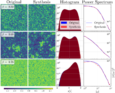
We evaluate the wavelet packet model at three different temperatures, which have different statistical properties: $\beta=0.50$, the “disorganized” state, $\beta=0.68\approx\beta_{c}$ the critical point, and $\beta=0.76$ the “organized” state. The computational efficiency of our approach enables generating high-resolution $128\times 128$ images, as opposed to $32\times 32$ in Marchand et al. (2022). Indeed, learning the model parameters for $64\times 64$ images with score matching takes seconds on GPU, whereas doing the same with maximum likelihood takes hours on CPU (as sequential MCMC steps are not easily parallelized). The generated samples are shown in Figure 3 and are qualitatively indistinguishable from the training data. The experimental setting is detailed in Appendix C.

A distribution $p(x)$ having a scalar potential energy (11) is a maximum-entropy distribution constrained by second-order moments and hence by the power spectrum, and by the marginal distribution of all $x[i]$. These statistics specify the matrix $K$ and the scalar potential $v(t).$ Our model $p_{\theta}$ also has a scalar potential energy in this case. To guarantee that $p_{\theta}=p$, it is thus sufficient to show that they have the same power spectrum and same marginal distributions. We perform a quantitative validation of generated samples by comparing their marginal densities and Fourier spectrum with the training data. Figure 3 shows that these statistics are well recovered by our model.

Figure 3: Comparison between training and generated samples for $\varphi^{4}$ energies. In columns: training samples, generated samples, histograms of marginal distributions $p(x[i])$ and power spectrum. In rows: disorganized state $\beta=0.50$, critical point $\beta=0.68\approx\beta_{c}$, and organized state $\beta=0.76$.

4.2 Conditional Log-Concavity

We numerically verify that $\varphi^{4}$ at critical temperature is CSLC (Definition 2.1), with appropriate wavelet packet projectors. It amounts to verifying that the eigenvalues of the conditional Hessian $\nabla^{2}_{\bar{x_{j}}}\bar{E}_{\bar{\theta}_{j}}(x_{j},\bar{x}_{j})$ are positive for all $x_{j}$ and $\bar{x}_{j}$. We can restrict $x_{j}$ to typical samples from $p(x_{j})$. However, it is important that the Hessian be positive even for $\bar{x}_{j}$ outside of the support of $p(\bar{x}_{j}|x_{j})$. Indeed, negative eigenvalues occur at local directional maxima of the energy, rather than minima which would correspond to most likely samples. We thus evaluate the Hessian at $\bar{x}_{j}=0$, which is expected to be such an adversarial point.

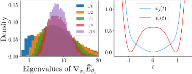
Figure 4 shows distributions of eigenvalues of $\nabla^{2}_{\bar{x}_{j}}\bar{E}_{\bar{\theta}_{j}}$ for decompositions $(\bar{G}_{j},G_{j})$ of various frequency bandwidths. It shows that the smallest eigenvalues become larger and eventually cross zero as the frequency bandwidth of $\bar{G}_{j}$ becomes narrower, as predicted by Proposition 3.1. Furthermore, the condition number of the Hessian becomes smaller as eigenvalues concentrate towards their mean.

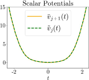
As shown in Equation 12, both the quadratic part $K$ and the scalar potential $v$ contribute to the Hessian. As a way to visualize both contributions, we define the equivalent scalar potential $v^{0}$ as $v^{0}(t)=v(t)+\frac{\operatorname{Tr}(K)}{2d}t^{2}$. It corresponds to extracting the mean quadratic value $\operatorname{Tr}(K)/2d\,\mathopen{}\mathclose{{}\left\lVert x}\right\rVert^{2}$ from the quadratic part and reinterpreting it as a scalar potential. This allows visualizing the average energy on a pixel value when neglecting spatial correlations. The right panel of Figure 4 compares these equivalent scalar potentials for the energy $E_{j}$ of $x_{j}$ and the conditional energy $\bar{E}_{j}$. It shows that the non-convex double-well potential in the global energy becomes convex after the conditioning. It verifies Proposition 3.1, as the mean quadratic value becomes larger when we restrict $K$ to a subspace of high-frequency signals.

Figure 4: Conditional strong log-concavity of $\varphi^{4}$ at critical temperature. All scales $j$ yield similar results. Left: distribution of eigenvalues of $\nabla^{2}_{\bar{x}_{j}}\bar{E}_{\bar{\theta}_{j}}$ for different frequency bandwidths ($j=1$ is shown). Right: equivalent scalar potentials $v_{j}$ and $\bar{v}_{j}$ ($j=3$ is shown).

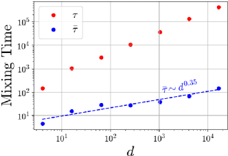
We also verify the sampling efficiency predicted by Proposition 2.2. As we cannot evaluate the $\mathrm{KL}$ divergences $\bar{\epsilon}_{j}^{S}$, we rather compute the decorrelation mixing time $\bar{\tau}$, a measure of the number of steps of conditional MALA to reach a given fixed error threshold averaged over all scales $j$. The precise definition is given in Section C.3. We compare it with the decorrelation mixing time $\tau$ of MALA on the non-convex global energy $E$.

Sampling maps of size $\sqrt{d}\times\sqrt{d}$ from the global $\varphi^{4}$ energy $E$ at the critical temperature requires a number of steps $\tau\sim d^{1.0}$ (Zinn-Justin, 2021). This phenomena is known as critical slowing down (Podgornik, 1996; Sethna, 2021), a consequence of long-range correlations. We numerically show that our algorithm does not suffer from it. Figure 5 indeed demonstrates an empirical scaling $\bar{\tau}\sim d^{0.35}$. Note that this is not directly comparable with Proposition 2.2 as the decorrelation mixing time defines a different convergence rate than the $\mathrm{KL}$ mixing time.

Figure 5: Mixing times for direct ($\tau$) and conditional ($\bar{\tau}$) sampling for $\varphi^{4}$ at critical temperature.

4.3 Application to Cosmological Data

We now apply our algorithm to generate high-resolution weak lensing convergence maps (Bartelmann & Schneider, 2001; Kilbinger, 2015) with an explicit probability model. Weak lensing convergence maps measure the bending of light near large gravitational masses on two-dimensional slices of the universe. We used simulated convergence maps computed by the Columbia lensing group (Zorrilla Matilla et al., 2016; Gupta et al., 2018) as training data. They simulate the next generation outer-space telescope Euclid of the European Space Agency (Laureijs et al., 2011), which will be launched in 2023 to accurately determine the large scale geometry of the universe governed by dark matter. Estimating the probability distribution of such maps is therefore an outstanding problem (Marchand et al., 2022). We demonstrate that the CSLC property is surprisingly verified in this real-world example, and can be used to efficiently model and generate these complex fields.

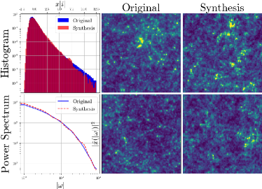
We use the same models and algorithms as for the $\varphi^{4}$ energy. The experimental setting is detailed in Appendix C. Figure 6 shows that our generated samples are visually highly similar to the training data. Quantitatively, they have nearly the same power spectrum. The marginal distribution of all $x[i]$ are also nearly the same, with a long tail corresponding to high amplitude peaks, which are typically difficult to reproduce. As opposed to microcanonical simulations with moment-matching algorithms (Cheng & Ménard, 2021), we compute an explicit probability distribution model, which is exponential. As a maximum-entropy model, it has a higher entropy than the true distribution, and therefore does not suffer from lack of diversity. By relying on the CSLC property, we can use the fast score-matching algorithm and compute $128\times 128$ images, at four times the $32\times 32$ resolution than with a maximum-likelihood algorithm used in Marchand et al. (2022).

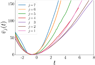
Figure 7 shows the equivalent scalar potentials of the conditional energies at all scales, which are all convex and thus verify the CSLC property of weak lensing model. It demonstrates that this property can be used to efficiently model and generate high-resolution complex data.

Figure 6: Comparison between training and generated samples for weak-lensing maps. Upper left: histograms of marginal distributions $p(x[i])$. Lower left: power spectrum. Center: training samples. Right: generated samples.

Figure 7: Equivalent scalar potentials $\bar{v}_{j}$ at each scale $j$ for weak-lensing maps (normalized for viewing purposes).

5 Discussion

We introduced conditionally strongly log-concave (CSLC) models and proved that they lead to efficient learning with score matching and sampling with MALA, while controlling errors. These models rely on iterated orthogonal projections of the data that are adapted to its distribution. We showed mathematically and numerically that complex multiscale physical fields satisfy the CSLC property with wavelet packet projectors. The argument is general and relies on the presence of a quadratic (kinetic) energy term which ensures strong log-concavity at high-frequencies. It provides high-quality and efficient generation of high-resolution fields even when the underlying distribution is unknown. The CSLC property guarantees diverse generations without memorization issues, which is critical in scientific applications.

CSLC models can be extended by introducing latent variables. The guarantees of Section 2 extend to the case where the data is a marginal of a CSLC distribution. A notable example is a score-based diffusion model, for which the data $x=x_{0}$ is a marginal of a higher-dimensional process $(x_{t})_{t}$ whose conditionals $p(x_{t-\delta}|x_{t})$ are approximately Gaussian white when $\delta$ is small, thus introducing a tradeoff between the number of terms in the CSLC decomposition and the condition number of its factors. Score diffusion is a generic transformation, but it assumes that the score $\nabla_{x_{t}}\log p(x_{t})$ can be estimated with deep networks at any $t\geq 0$ (Song et al., 2021; Ho et al., 2020). For high-resolution images, the score estimation often uses conditional multiscale decompositions with or without wavelet transforms (Saharia et al., 2021; Ho et al., 2022; Dhariwal & Nichol, 2021; Guth et al., 2022). Understanding the log-concavity properties of natural image distributions under such transformations is a promising research avenue to understand the effectiveness of score-based diffusion models.

[sections] [sections]l1

Appendix A Definition of Wavelet Packet Projectors

The fast wavelet transform (Mallat, 1989) splits a signal in frequency into two orthogonal coarser signals, using two orthogonal conjugate mirror filters $g$ and $\bar{g}$.

We review the construction of such filters in Section A.1. A description of the fast wavelet transform is then given in Section A.2. Finally, we define in Section A.3 the wavelet packet (Coifman et al., 1992) projectors $({G}_{j},\bar{G}_{j})$ used in the numerical section 3.

A.1 Conjugate Mirror Filters

Conjugate mirror filters $g$ and $\bar{g}$ satisfy the following orthogonal and reconstruction conditions:

$$\begin{array}[]{ll}g^{\mathrm{T}}\bar{g}=\bar{g}^{\mathrm{T}}g=0,\\ g^{\mathrm{T}}g+\bar{g}^{\mathrm{T}}\bar{g}=\mathrm{Id}.\end{array}$$ (14)

In one dimension, the conditions (14) are satisfied (Mallat, 1989) by discrete filters $(g(n))_{n\in\mathbb{Z}},(\bar{g}(n))_{n\in\mathbb{Z}}$ whose Fourier transforms $\hat{g}(\omega)=\sum_{n}g(n)e^{-in\omega}$ and $\hat{\bar{g}}(\omega)=\sum_{n}g(n)e^{-in\omega}$ satisfy

$$\begin{array}[]{ll}|\hat{g}(\omega)|^{2}+|\hat{g}(\omega+\pi)|^{2}=2,\\ \hat{g}(0)=\sqrt{2},\\ \hat{\bar{g}}(\omega)=e^{-i\omega}\hat{g}(\omega+\pi).\par\end{array}$$ (15)

We first design a low-frequency filter $g$ such that $\hat{g}(\omega)$ satisfies (15), and then compute $\bar{g}$ with

$$\begin{array}[]{ll}\bar{g}(n)=(-1)^{1-n}g(1-n).\end{array}$$ (16)

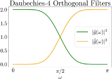
The choice of a particular low pass filter $g$ is a trade-off between a good localization in space and a good localization in the Fourier frequency domain. Choosing a perfect low-pass filter $g(\omega)=\mathds{1}_{\omega\in[-\pi/2,\pi/2]}$ leads to Shannon wavelets, which are well localized in the frequency domain but have a slow decay in space. On the opposite, a Haar wavelet filter $g(n)=\sqrt{2}\,\mathds{1}_{n\in\{0,1\}}$ has a small support in space but is poorly localized in frequency. Daubechies filters (Daubechies, 1992) provide a good joint localization both in the spatial and Fourier domains. The Daubechies-$4$ wavelet is shown in Figure 8.

Figure 8: Fourier transform of Daubechies-4 orthogonal filters $\hat{g}(\omega)$ (in green) and $\hat{\bar{g}}(\omega)$ (in orange).

In two dimensions (for images), wavelet filters which satisfy the orthogonality conditions in (14) can be defined as separable products of the one-dimensional filters $g$ and $\bar{g}$ (Mallat, 2009), applied on each coordinate. It defines one low-pass filter $g_{2}$ and $3$ high-pass filters $\bar{g}_{2}=(\bar{g}_{2}^{k})_{1\leq k\leq 3}$:

$$\begin{array}[]{c}g_{2}(n_{1},n_{2})=g(n_{1})g(n_{2}),\\ \bar{g}_{2}^{1}(n_{1},n_{2})=g(n_{1})\bar{g}(n_{2}),\\ \bar{g}_{2}^{2}(n_{1},n_{2})=\bar{g}(n_{1})g(n_{2}),\\ \bar{g}_{2}^{3}(n_{1},n_{2})=\bar{g}(n_{1})\bar{g}(n_{2}).\end{array}$$ (17)

For simplicity we shall write $g$ and $\bar{g}$ the filters $g_{2}$ and $\bar{g}_{2}$. $\bar{g}$ outputs the concatenation of the 3 filters $\bar{g}_{2}^{k}$.

A.2 Orthogonal Frequency Decomposition

We introduce the orthogonal decomposition of a signal $x_{j-1}$ with the low pass filter $g$ and the high pass filter $\bar{g}$, followed by a sub-sampling. It outputs $(x_{j},\bar{x}_{j})$, which has the same dimension as $x_{j-1}$, defined in one dimension by

$$\begin{array}[]{ll}x_{j}[p]=\sum\limits_{n\in\mathbb{R}^{2}}g[n-2p]x_{j-1}[n],\\ \bar{x}_{j}[p]=\sum\limits_{n\in\mathbb{R}^{2}}\bar{g}[n-2p]x_{j-1}[n].\end{array}$$ (18)

The inverse transformation is

$$\begin{array}[]{l}x_{j}[p]=\sum\limits_{n\in\mathbb{R}^{2}}g[p-2n]x_{j+1}[n]+\sum\limits_{n\in\mathbb{R}^{2}}\bar{g}[p-2n]\bar{x}_{j+1}[n].\end{array}$$ (19)

The orthogonal frequency decomposition in two dimensions is defined similarly. It decomposes a signal $x$ of size $\sqrt{d}\times\sqrt{d}$ into a low frequency signal and $3$ high frequency signals, each of size $\frac{\sqrt{d}}{2}\times\frac{\sqrt{d}}{2}$.

A.3 Wavelet Packet Projectors

An orthogonal frequency decomposition projects a signal into high and low frequency domains. In order to refine the decomposition (by separating different frequency bands), wavelet packets projectors are obtained by cascading this orthogonal frequency decomposition.

The usual fast wavelet transform starts from a signal $\bar{x}_{0}$ of dimension $d$, decomposes it into a low-frequency $x_{1}$ and a high frequency $\bar{x}_{1}$, and then iterates this decomposition on the low-frequency $x_{1}$ only. It iteratively decomposes $x_{j-1}$ into the lower frequencies $x_{j}$ and the high-frequencies $\bar{x}_{j}$. The resulting orthogonal wavelet coefficients are $(\bar{x}_{j},x_{J})_{1\leq j\leq J}$. The resulting decomposition remains of dimension $d$.

To obtain a finer frequency decomposition, we use the $M$-band wavelet transform (Mallat, 2009), a particular case of wavelet packets (Coifman et al., 1992). It first applies the fast wavelet transform to the signal, and obtains $(\bar{x}_{j},x_{J})_{1\leq j\leq J}$. Each high-frequency output $\bar{x}_{j}$ undergoes an orthogonal decomposition using $g$ and $\bar{g}$. Then both outputs of the decomposition are again decomposed, and so on, $(M-1)$-times. The coefficients are then sorted according to their frequency support, and also labeled as $(\bar{x}_{j},x_{J})_{1\leq j\leq J^{\prime}}$, with $J^{\prime}=J2^{M-1}$, also referred to as $J$ in the main text.

The wavelet packet decomposition corresponds to first decomposing the frequency domain dyadically into octaves, and then each dyadic frequency band is further decomposed into $2^{M-1}$ frequency annuli. We say this decomposition corresponds to a $1/2^{M-1}$ octave bandwidth. Precisely, if $j=j^{\prime}2^{M-1}+r$, then $\bar{x}_{j}$ has a frequency support over an annulus in the frequency domain, with frequencies with modulus of order $2^{-j^{\prime}}\pi(1-{2^{-M+1}}(r-1/2))$. A two-dimensional visualization of the frequency domain can be found in Figure 2, for $M=1$ and $M=2$, corresponding to $1$ and $1/2$ octave bandwidths.

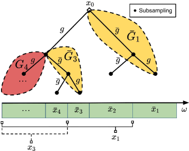
Figure 9 shows the iterative use of $g$ and $\bar{g}$ used to obtain the decomposition, in one dimension, for $M=2$. Note that the filters $\bar{g}$ and $g$ successively play the role of low- and high-pass filters because of the subsampling (Mallat, 2009).

We now introduce the corresponding orthogonal projectors $G_{j}$ and $\bar{G}_{j}$, defined such that

$$\begin{array}[]{ll}\bar{x}_{j}=\bar{G}_{j}x_{j-1},\\ x_{j}=G_{j}x_{j-1},\par\end{array}$$ (20)

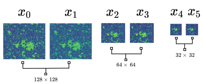
where the $(\bar{x}_{j})_{j}$, sorted in frequency, have been obtained trough the $M$-band wavelet transform, as described above, and $x_{j}$ refers to the signal reconstructed using $(x_{J},\bar{x}_{j^{\prime}})_{j^{\prime}\geq j+1}$. Let us emphasize that the image $x_{j-1}$ is reconstructed from $x_{j}$ and the higher frequencies $\bar{x}_{j}$, and defined on a spatial grid which is either the same as $x_{j}$ or twice larger. For $M=2$, Figure 10 shows that $x_{0}$ and $x_{1}$ are defined on the same grid, although $x_{1}$ has a lower-frequency support. Similarly $x_{2}$ and $x_{3}$ are both represented on the same grid, which is twice smaller, and so on.

The orthogonal projectors satisfy $G_{j}^{\mathrm{T}}G_{j}+\bar{G}_{j}^{\mathrm{T}}\bar{G}_{j}=\mathrm{Id}$. We then have the following inverse formula:

$$\begin{array}[]{l}x_{j-1}=G_{j}^{\mathrm{T}}x_{j}+\bar{G}_{j}^{\mathrm{T}}\bar{x_{j}}.\end{array}$$ (21)

This decomposition using $G_{j}$ and $\bar{G}_{j}$ recursively splits the signal in frequencies, from high to low frequencies.

Figure 9: In one dimension, a wavelet packet transform is obtain by cascading filterings and subsamplings with the filters $g$ and $\bar{g}$ along a binary splitting tree which outputs $x_{J}$ and $\bar{x}_{j}$ for $j\geq J$.

Figure 10: Low-frequency maps $x_{j}$ for $M=2$ for a $\varphi^{4}$ realization.

Appendix B Score Matching and MALA Algorithms for CSLC Exponential Families

B.1 Multiscale Energies

This section introduces the explicit parametrization of the energies $\bar{E}_{\bar{\theta}_{j}}$ and $E_{\theta_{J}}$.

The conditional energies $\bar{E}_{\bar{\theta}_{j}}(x_{j},\bar{x}_{j})$ are defined with a bilinear term which represents the interaction between $x_{j}$ and $\bar{x}_{j}$ and a scalar potential:

$$\bar{E}_{\bar{\theta}_{j}}(x_{j},\bar{x}_{j})=\frac{1}{2}\bar{x}_{j}^{\mathrm{T}}\bar{K}_{j}\bar{x}_{j}+\sum\limits_{l>j}\bar{x}_{j}^{\mathrm{T}}\bar{K}^{\prime}_{l,j}\bar{x}_{j+l}+\sum_{i}\bar{v}_{j}(x_{j-1}[i]),$$ (22)

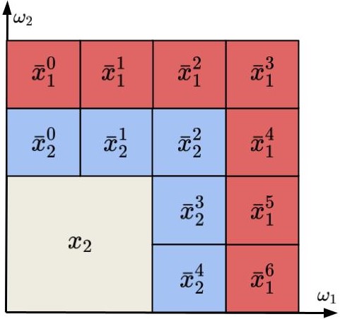
with $x_{j-1}=\bar{G}_{j}^{\mathrm{T}}\bar{x}_{j}+G_{j}^{\mathrm{T}}x_{j}.$ Equation 22 is an equivalent reparametrization of Equation 13. Considering $(\bar{x}_{l})_{l>j}$ instead of $x_{j}$ allows fixing some coefficients of the $\bar{K}^{\prime}_{l,j}$ to zero instead of learning them. First, we set $\bar{K}^{\prime}_{l,j}=0$ if $\bar{x}_{j}$ and $\bar{x}_{j+l}$ are not defined on the same spatial grid. In the sequel, sums over $l$ only refer to theses terms, which differ depending on the wavelet decomposition. We enforce spatial stationarity by averaging the bilinear interaction terms across space. We further kept only the non-negligible terms which correspond to neighboring frequencies and neighboring spatial locations. As displayed in Figure 11, $\bar{x}_{j}$ is composed of sub-bands $\bar{x}_{j}^{k}$. We kept the interaction terms $\bar{x}_{j}^{k}[i]\bar{x}_{j+l}^{k+\delta k}[i+\delta i]$ for $l\in\{0,1\}$, $\delta k\in\{0,1\}$, and $\delta i\in\{0,1,2,3,4\}^{2}$, which correspond to local interactions in both space and frequency.

Figure 11: Sub-bands of $\bar{x}_{j}$ for a wavelet packet decomposition with a half-octave bandwidth.

The scalar potential $\bar{v}_{j}(t)$ is decomposed on a family of predefined functions $\rho_{k,j}(t)$:

$$\bar{v}_{j}(t)=\sum\limits_{k}\bar{\alpha}_{k,j}\,{\rho}_{k,j}(t).$$ (23)

${\rho}_{j,k}$ is defined in order to expand the scalar potential $\bar{v}_{j}$ which captures the marginal distributions of the $x_{j-1}[i]$, which do not depend on $i$ due to stationarity. We divide this marginal into $N$ quantiles. Each ${\rho}_{k,j}$ is chosen to be a regular bump function having a finite support on the $k$-th quantile. This parametrization performs a pre-conditioning of the score matching Hessian.

Let $\rho$ be a bump function with a support in $[-{1}/{2},{1}/{2}]$. For each $j$, let $a_{j,k}$ and $l_{j,k}$ be respectively the center and width of the $k$-th quantile of the marginal distribution of $\bar{x}_{j}$, we define

$${\rho}_{k,j}(t)=\,l_{k}\sqrt{N}\,\rho\mathopen{}\mathclose{{}\left(\frac{t-a_{j,k}}{l_{j,k}}}\right),$$ (24)

with the condition

$$\mathopen{}\mathclose{{}\left\lVert\rho^{\prime}}\right\rVert_{2}^{2}=\frac{1}{\mathopen{}\mathclose{{}\left\lVert\bar{G}_{j}}\right\rVert_{2}^{2}},$$ (25)

in order to balance the magnitude of the scalar potentials with the quadratic potentials.

The potential vector is thus

$$\bar{\Phi}_{j}(x_{j},\bar{x}_{j})=\mathopen{}\mathclose{{}\left(\sum\limits_{i}\bar{x}_{j}^{k}[i]\bar{x}_{j+l}^{k+\delta k}[i+\delta_{i}],\sum\limits_{i}\rho_{k^{\prime},j}(x_{j-1}[i])}\right)_{0\leq l\leq 1,0\leq\delta k\leq 1,0\leq\delta_{i}\leq 4,1\leq k^{\prime}\leq N}.$$ (26)

Similarly, we define $E_{\theta_{J}}$ as the sum of a quadratic energy and a scalar potential:

$${E}_{{\theta}_{J}}(x_{J})=\frac{1}{2}x_{J}^{\mathrm{T}}K_{J}x_{J}+\sum_{i}v_{J}(x_{J}[i]).$$ (27)

The bilinear interaction terms are averaged across space to enforce stationarity. The scalar potential $v_{J}(t)$ is also decomposed over a family of predefined functions $\rho_{k,J}(t)$:

$$v_{J}(t)=\sum\limits_{k}\alpha_{k,J}\,\rho_{k,J}(t),$$ (28)

defined similarly as above. This yields a potential vector

$$\Phi_{J}(x_{J})=\mathopen{}\mathclose{{}\left(\sum_{i}x_{J}[i]x_{J}[i+\delta_{i}],\rho_{k,J}(x_{J})}\right)_{0\leq\delta i\leq 4,1\leq k\leq N},$$ (29)

leading to

$${E}_{{\theta}_{J}}(x_{J})=\theta_{J}^{\mathrm{T}}\Phi_{J}(x_{J}),$$ (30)

with $\theta_{J}=(K_{J},\alpha_{k,J})_{k}$.

B.2 Pseudocode

The procedure to learn the parameters $(\bar{\theta}_{j})_{j}$ of the conditional energies $\bar{E}_{\bar{\theta}_{j}}(x_{j},\bar{x}_{j})$ by score matching is detailed in Algorithm 1. The procedure to generate samples from the distribution $p_{\theta}(x)$ with MALA is detailed in Algorithm 2.

Algorithm 1 Score matching for exponential families with CSLC distributions

0:  Training samples $(x^{i})_{1\leq i\leq n}$.

  Initialize $x^{i}_{0}=x^{i}$ for $1\leq i\leq n$.

  for $j=1$ to $J$ do

     Decompose $x_{j}^{i}\leftarrow G_{j}x_{j-1}^{i}$ and $\bar{x}_{j}^{i}\leftarrow\bar{G}_{j}x_{j-1}^{i}$ for $1\leq i\leq n$.

     Compute the score matching quadratic term ${H}_{j}\leftarrow\frac{1}{n}\sum_{i=1}^{n}{\nabla_{\bar{x}_{j}}\bar{\Phi}_{j}(x^{i}_{j},\bar{x}^{i}_{j})\nabla_{\bar{x}_{j}}\bar{\Phi}_{j}(x^{i}_{j},\bar{x}^{i}_{j})^{\mathrm{T}}}\in{\mathbb{R}}^{m\times m}$.

     Compute the score matching linear term ${g}_{j}\leftarrow\frac{1}{n}\sum_{i=1}^{n}{\Delta_{\bar{x}_{j}}\bar{\Phi}_{j}(x^{i}_{j},\bar{x}^{i}_{j})}\in{\mathbb{R}}^{m}$.

     Set $\bar{\theta}_{j}\leftarrow H_{j}^{-1}g_{j}$.

  end for

  return  Model parameters $(\bar{\theta}_{j})_{j}$.

Algorithm 2 MALA sampling from CSLC distributions

0:  Model parameters $(\bar{\theta}_{j})_{j}$, an initial sample $x_{J}$ from $p(x_{J})$, step sizes $(\delta_{j})_{j}$, number of steps $(T_{j})_{j}$.

  for $j=J$ to $1$ do

     Initialize $\bar{x}_{j,0}=0$.

     for $t=1$ to $T_{j}$ do

        Sample $\bar{y}_{j,t}\sim\mathcal{N}\mathopen{}\mathclose{{}\left(\bar{x}_{j,t-1}-\delta_{j}\nabla_{\bar{x}_{j}}\bar{E}_{\bar{\theta}_{j}}(x_{j},\bar{x}_{j,t-1}),2\delta_{j}\mathrm{Id}}\right)$.

        Set $a=\mathopen{}\mathclose{{}\left\lVert\nabla_{\bar{x}_{j}}\bar{E}_{\bar{\theta}_{j}}(x_{j},\bar{y}_{j,t}))}\right\rVert^{2}+\mathopen{}\mathclose{{}\left\lVert\nabla_{\bar{x}_{j}}\bar{E}_{\bar{\theta}_{j}}(x_{j},\bar{x}_{j,t-1}))}\right\rVert^{2}$.

        Set $b=\mathopen{}\mathclose{{}\left\langle\bar{y}_{j,t}-\bar{x}_{j,t-1},\nabla_{\bar{x}_{j}}\bar{E}_{\bar{\theta}_{j}}(x_{j},\bar{y}_{j,t})-\nabla_{\bar{x}_{j}}\bar{E}_{\bar{\theta}_{j}}(x_{j},\bar{x}_{j,t-1})}\right\rangle$.

        Set $c=\bar{E}_{\bar{\theta}_{j}}(x_{j},\bar{y}_{j,t})-\bar{E}_{\bar{\theta}_{j}}(x_{j},\bar{x}_{j,t-1})$.

        Compute acceptance probability $p=\exp\mathopen{}\mathclose{{}\left(-\frac{\delta_{j}}{4}a+\frac{1}{2}b-c}\right)$.

        Set $\bar{x}_{j,t}=\bar{y}_{j,t}$ with probability $p$ and $\bar{x}_{j,t}=\bar{x}_{j,t-1}$ with probability $1-p$.

     end for

     Reconstruct $x_{j-1}=G_{j}^{\mathrm{T}}x_{j}+\bar{G}_{j}^{\mathrm{T}}\bar{x}_{j,T_{j}}$.

  end for

  return  a sample $x_{0}$ from $\hat{p}_{\theta}(x)$.

Appendix C Experimental Details

C.1 Datasets

Simulations of $\mathbf{\varphi^{4}}$.

We used samples from the $\varphi^{4}$ model generated using a classical MCMC algorithm, for 3 different temperatures, at the critical temperature $\beta_{c}\approx 0.68$, above the critical temperature at $\beta=0.50<\beta_{c}$, and below the critical temperature at $\beta=0.76>\beta_{c}$. For $\beta=0.76$, we break the symmetry and only generate samples with positive mean. For each temperature, we generate $10^{4}$ images of size $128\times 128$.

Weak lensing.

We used down-sampled versions of the simulated convergence maps from the Columbia Lensing Group (http://columbialensing.org/; Zorrilla Matilla et al., 2016; Gupta et al., 2018). Each map, originally of size $1024\times 1024$, is downsampled twice with local averaging. We then extract random patches of size $128\times 128$.

To pre-process the data, we subtract the minimum of the pixel values over the entire dataset, and then take the square root. This process is reversed after generating samples. We also do not consider the outliers (less than $1\%$ of the dataset) with pixels above a certain cutoff, in order to reduce the extent of the tail and attenuate weak lensing peaks. Our dataset is made of $\simeq 4\times 10^{3}$ images.

C.2 Experimental Setup

Wavelet filter.

We used the Daubechies-4 wavelet (Daubechies, 1992), see the filter in Figure 8.

Wavelet packets.

We implemented wavelet packets in PyTorch, inspired from the PyWavelets software (Lee et al., 2019). The source code is available at https://github.com/Elempereur/WCRG.

Score matching.

We pre-condition the score matching Hessian $H_{j}$ by normalizing its diagonal before computing $H_{j}^{-1}g_{j}$ in Algorithm 1. After this normalization, we obtain condition numbers $\kappa_{\bar{\theta}_{j}}$ which satisfy $\kappa_{\bar{\theta}_{j}}\leq 2\times 10^{3}$ at all $j$.

Sampling.

The MALA step sizes $\delta_{j}$ are adjusted to obtain an optimal acceptance rate of $\approx 0.57$. Depending on the scale $j$, the stationary distribution is reached in $T_{j}\approx 20$–$400$ iterations from a white noise initialization. We used a qualitative stopping criterion according to the quality of the matching of the histograms and power spectrum.

C.3 Mixing Times in MALA

Sampling from $p_{\theta}$ requires sampling from $p_{\theta_{J}}$, and then conditionally sampling from $p_{\bar{\theta}_{j}}(\bar{x}_{j}|x_{j})$. This last step is performed with a Markov chain whose stationary distribution is $p_{\bar{\theta}_{j}}(\bar{x}_{j}|x_{j})$ for a given $x_{j}$. It generates successive samples $\bar{x}_{j}(t)$ where $t$ is the the step number in the Markov chain.

We introduce the conditional auto-correlation function:

$$A_{j}(t)=\frac{\mathbb{E}\mathopen{}\mathclose{{}\left[\mathopen{}\mathclose{{}\left(\bar{x}_{j}(t)-\mathbb{E}[\bar{x}_{j}\,|\,x_{j}]}\right)\mathopen{}\mathclose{{}\left(\bar{x}_{j}(0)-\mathbb{E}[\bar{x}_{j}\,|\,x_{j}]}\right)}\right]}{\mathbb{E}[\delta\bar{x}_{j}^{2}]}.$$

The expected value $\mathbb{E}$ is taken with respect to both $x_{j}$ and the sampled $\bar{x}_{j}$. $A_{j}(t)$ has an exponential decay. Let $\bar{\tau}_{j}$ be the mixing time defined as the time it takes for the Markov chain to generate two independent samples:

$$A_{j}(t)\approx A_{j}(0)\exp\mathopen{}\mathclose{{}\left(-\frac{t}{\bar{\tau}_{j}}}\right).$$

$\bar{\tau}_{j}$ is computed by regressing $\log(A_{j}(t))$ over $t$.

Each iteration of MALA with $p_{\bar{\theta}_{j}}(\bar{x}_{j}\mid x_{j})$ computes a gradient of size $\bar{d}_{j}$. In order to estimate the real computational cost of the sampling of $p_{\theta}$, we average $\bar{\tau}_{j}$ proportionally to the dimension $\bar{d}_{j}$:

$$\bar{\tau}=\sum\limits_{j=1}^{J}\frac{{\bar{d}_{j}}}{d}\bar{\tau}_{j}+{\tau}_{J}\frac{d_{J}}{d},$$

where $d$ is the dimension of $x$.

Appendix D Energy Estimation with Free-Energy Modeling

This section explains how to recover an explicit parametrization of the negative log-likelihood $-\log p_{\theta}$ from the parameterized energies $\bar{E}_{\bar{\theta}_{j}}$. We introduce a parameterization of the normalization constant of the Gibbs energies for each $j$ and describe an efficient score-matching algorithm to learn the parameters. This leads to a decomposition of the negative log-likelihood $-\log p_{\theta}$ over scales.

D.1 Free-Energy Score Matching

From the decomposition

$$p_{\theta}(x)=p_{\theta_{J}}(x_{J})\prod_{j=1}^{J}p_{\bar{\theta}_{j}}(\bar{x}_{j}|x_{j}),$$

we obtain

$$-\log p_{\theta}(x)=E_{\theta_{J}}(x_{J})+\sum_{j=1}^{J}\mathopen{}\mathclose{{}\left(\bar{E}_{\bar{\theta}_{j}}(x_{j},\bar{x}_{j})+\log\bar{Z}_{\bar{\theta}_{j}}(x_{j})}\right)+\mathrm{cst},$$ (31)

where $\bar{Z}_{\bar{\theta}_{j}}(x_{j})$ is the normalization constant for $\bar{E}_{\bar{\theta}_{j}}(x_{j},\bar{x}_{j})$. To retrieve the global negative log-likelihood $-\log p_{\theta}(x)$, we thus compute an approximation of $-\log\bar{Z}_{\bar{\theta}_{j}}(x_{j})$ with a parametric family $F_{\tilde{\theta}_{j}}$.

The parameters $\tilde{\theta}_{j}$ of the approximation of the normalizing factors $\bar{Z}_{\tilde{\theta}_{j}}$ can be learned in a manner similar to denoising score matching. Indeed, using the identity

$$-\nabla_{x_{j}}\log\bar{Z}_{\bar{\theta}_{j}}(x_{j})=\mathbb{E}\mathopen{}\mathclose{{}\left[\nabla_{x_{j}}\bar{E}_{\bar{\theta}_{j}}(x_{j},\bar{x}_{j})\,|\,x_{j}}\right],$$

which can be proven by a direct computation of the gradient, the parameters $\tilde{\theta}_{j}$ can be estimated by minimizing

$$\tilde{\ell}_{j}(\tilde{\theta}_{j})=\mathbb{E}\mathopen{}\mathclose{{}\left[\mathopen{}\mathclose{{}\left\lVert\nabla_{x_{j}}F_{\tilde{\theta}_{j}}-\nabla_{x_{j}}\bar{E}_{\bar{\theta}_{j}}}\right\rVert^{2}}\right].$$ (32)

For an exponential model $F_{\tilde{\theta}_{j}}=\tilde{\theta}_{j}^{\mathrm{T}}\tilde{\Phi}_{j}$ with a fixed potential vector $\tilde{\Phi}_{j}$, Equation 32 is quadratic in $\tilde{\theta}$ and admits a closed-form solution:

$$\tilde{\theta}_{j}=\mathbb{E}\mathopen{}\mathclose{{}\left[\nabla_{x_{j}}\tilde{\Phi}_{j}\nabla_{x_{j}}\tilde{\Phi}_{j}^{\mathrm{T}}}\right]^{-1}\mathbb{E}\mathopen{}\mathclose{{}\left[\nabla_{x_{j}}\tilde{\Phi}_{j}\nabla_{x_{j}}\bar{E}_{\bar{\theta}_{j}}}\right].$$

We finally obtain the energy decomposition

$$-\log p_{\theta}(x)=E_{\theta_{J}}(x_{J})+\sum_{j=1}^{J}\mathopen{}\mathclose{{}\left(\bar{E}_{\bar{\theta}_{j}}(x_{j},\bar{x}_{j})-F_{\tilde{\theta}_{j}}(x_{j})}\right)+\mathrm{cst}.$$ (33)

This score-based method is much faster and simpler to implement than likelihood-based methods such as the thermodynamic integration of Marchand et al. (2022), which requires generation of many samples while varying the parameters $\bar{\theta}_{j}$ of the conditional energy $\bar{E}_{\bar{\theta}_{j}}$.

D.2 Parameterized Free-Energy Models

The potential vector $\tilde{\Phi}_{j}$ is modeled in the class of Equation 11, following Marchand et al. (2022) and similarly to Section B.1:

$$F_{\tilde{\theta}_{j}}(x_{j}) =\frac{1}{2}x_{j}^{\mathrm{T}}\tilde{K}_{j}x_{j}+\tilde{V}_{j}(x_{j})+\sum\limits_{i}\tilde{v}_{j}(x_{j}[i])$$

$$\tilde{v}_{j}(t) =\sum\limits_{k}\tilde{\alpha}_{j,k}\tilde{\rho}_{j,k}(t),$$

which gives $\tilde{\theta}_{j}=(\tilde{K}_{j},\tilde{\alpha}_{j,k})_{k}$ and an associated potential vector

$$\tilde{\Phi}_{j}(x_{j})=\mathopen{}\mathclose{{}\left(\frac{1}{2}x_{j}x_{j}^{\mathrm{T}},\tilde{\rho}_{j,k}(x_{j})}\right)_{k}.$$

D.3 Multiscale Energy Decomposition

We now expand the models for the conditional energies $\bar{E}_{\bar{\theta}_{j}}$ and the so-called free energies $F_{\tilde{\theta}_{j}}$ in Equation 33. All the quadratic terms $(K_{J},\bar{K}_{j},\tilde{K}_{j})_{j}$ can be regrouped in an equivalent quadratic term $K$. We then have

$$-\log p_{\theta}(x) =\frac{1}{2}x^{\mathrm{T}}Kx+\sum\limits_{i}\mathopen{}\mathclose{{}\left[v_{J}(x_{J}[i])+\sum_{j=1}^{J}\mathopen{}\mathclose{{}\left(\bar{v}_{j}(x_{j-1}[i])-\tilde{v}_{j}(x_{j}[i])}\right)}\right]$$

$$=\frac{1}{2}x^{\mathrm{T}}Kx+\sum\limits_{i}\mathopen{}\mathclose{{}\left[\bar{v}_{1}(x_{0}[i])+\sum_{j=1}^{J}\mathopen{}\mathclose{{}\left(\bar{v}_{j+1}(x_{j}[i])-\tilde{v}_{j}(x_{j}[i])}\right)}\right],$$

with $\bar{v}_{J+1}=v_{J}$. This defines multiscale scalar potentials $V_{j}$:

$$\begin{array}[]{l}V_{j}=\bar{v}_{j+1}-\tilde{v}_{j},\\ V_{0}=\bar{v}_{1},\end{array}$$

such that we have the global negative log-likelihood or energy function:

$$-\log p_{\theta}(x)=\frac{1}{2}x^{\mathrm{T}}Kx+\sum_{j=0}^{J}\sum_{i}V_{j}(x_{j}[i]).$$

For $\varphi^{4}$ at critical temperature, as derived in (Marchand et al., 2022), the only non-zero scalar potential will be $V_{0}$. The other $V_{j}$ potentials are zero, up to a quadratic term.

As a numerical test, Figure 12 verifies that on $\varphi^{4}$ at critical temperature, $\bar{v}_{j+1}$ and $\tilde{v}_{j}$ indeed cancel out so that $V_{j}=0$ for $j>0$. In order to ensure that the quadratic difference mentioned above vanishes, we subtract to $\tilde{v}_{j}$ the quadratic interpolation of $\tilde{v}_{j}-\bar{v}_{j+1}$.

Figure 12: For $\varphi^{4}$ at $\beta_{c}$, the conditional potentials $\bar{v}_{j+1}$ and free-energy potential $\tilde{v}_{j}$ cancel out. Only $j=1$ is shown, other scales show similar behavior.

Appendix E Proofs of Section 2

E.1 Proof of Proposition 2.1

See 2.1

Proof.

We use the following decomposition of KL divergence in terms of conditional distributions:

Lemma E.1.

Let $p(x)=p(x_{J})\prod_{j=1}^{J}p(\bar{x}_{j}|x_{j})$ and $q(x)=q(x_{J})\prod_{j}q(\bar{x}_{j}|x_{j})$. We have $\mathrm{KL}(p\,\|\,q)=\sum_{j}\mathbb{E}_{x_{j}\sim p}\mathrm{KL}(p(\cdot|x_{j})\,\|\,q(\cdot|x_{j}))~{}.$

Using Lemma E.1 we obtain that $\mathrm{KL}(p\,\|\,p_{\theta})=\epsilon_{J}^{L}+\sum_{j}\bar{\epsilon}^{L}_{j}$ and $\mathrm{KL}(\hat{p}\,\|\,p_{\theta})=\epsilon_{J}^{S}+\sum_{j}\bar{\epsilon}^{L}Sj$. We conclude with the Pinsker inequality

$$\mathrm{TV}(\hat{p},p)\leq\mathrm{TV}(\hat{p},p_{\theta})+\mathrm{TV}({p}_{\theta},p)\leq\frac{1}{\sqrt{2}}\mathopen{}\mathclose{{}\left(\sqrt{\mathrm{KL}(p\,\|\,p_{\theta})}+\sqrt{\mathrm{KL}(\hat{p}\,\|\,p_{\theta})}}\right)~{}.$$

∎

Proof of Lemma E.1.

We proceed by induction over $J$. Observe that $\log p(x)=\log p(\bar{x}_{1}|x_{1})+\log p(x_{1})$, so

$$\mathrm{KL}(p\,\|\,q) =\mathbb{E}_{p}[\log(p)-\log(q)]$$

$$=\mathbb{E}_{p}[\log p(x_{1})-\log q(x_{1})]+$$

$$\mathbb{E}_{x_{1}\sim p(x_{1})}\mathbb{E}_{\bar{x}_{1}\sim p(\bar{x}_{1}|x_{1})}[\log p(\bar{x}_{1}|x_{1})-\log q(\bar{x}_{1}|x_{1})]$$

$$=\mathrm{KL}(p(x_{1})\,\|\,q(x_{1}))$$

$$+\mathbb{E}_{x_{1}\sim p(x_{1})}\mathrm{KL}(p(\cdot|x_{1})\,\|\,q(\cdot|x_{1}))~{}.$$

The first term $\mathrm{KL}(p(x_{1})\,\|\,q(x_{1}))$ now involves $J-1$ factors, and hence we can apply the induction step to conclude. ∎

E.2 Proof of Theorem 2.1

We will use a general concentration result of the empirical covariance for general distributions with mild moment assumptions (Vershynin, 2018), as well as anticoncentration properties of the random design (Mourtada, 2022). Together, they provide enough control on the probability tails so that the inverse covariance concentrates to the precision matrix in expectation.

Assumption E.1.

Let $X\in\mathbb{R}^{m\times d}$ be a random matrix. Assume that there exists $K\geq 1$ such that $\|X\|_{F}\leq K\mathbb{E}[\|X\|_{F}^{2}]^{1/2}$ almost surely.

Theorem E.1 (General Covariance Estimation with High Probability, (Vershynin, 2018, Theorem 5.6.1, Ex 5.6.4)).

Let $X\in\mathbb{R}^{m\times d}$ be a random matrix satisfying assumption E.1. Let $\Sigma=\mathbb{E}[XX^{\top}]$, and for any $n$ let $\hat{\Sigma}_{n}=\frac{1}{n}\sum_{i}X_{i}X_{i}^{\top}$ be the sample covariance matrix, where $X_{i}$ are $n$ iid copies of $X$. There exists an absolute constant $C$ such that for any $\delta>0$, it holds

$$\|\hat{\Sigma}_{n}-\Sigma\|\leq C\mathopen{}\mathclose{{}\left(\sqrt{\frac{K^{2}m(\log(m)+\log(2/\delta))}{n}}+\frac{K^{2}m(\log(m)+\log(2/\delta))}{n}}\right)\|\Sigma\|$$ (34)

with probability at least $1-\delta$.

Assumption E.2 (Moment Condition).

Assume that there exists $K_{X}$ and $K_{Y}$ such that $X:=(\nabla_{\bar{x}}\bar{\Phi}_{k}(\bar{x},x))_{k\leq m}\in\mathbb{R}^{m\times d}$, and $Y=(\Delta_{\bar{x}}\bar{\Phi}_{k}(\bar{x},x))_{k\leq m}\in\mathbb{R}^{m}$ satisfy Assumption E.1 with constants $K_{X}$ and $K_{Y}$ respectively, where $(\bar{x},x)\sim p(\bar{x},x)$.

Assumption E.3 (Anticoncentration Condition, (Mourtada, 2022, Assumption 1)).

The random matrix $X=(\nabla_{\bar{x}}\bar{\Phi}_{k}(\bar{x},x))_{k\leq m}\in\mathbb{R}^{m\times d}$ satisfies the following: there exists constants $C\geq 1$ and $\nu\in(0,1]$ such that for every $\theta\in\mathbb{R}^{m}\setminus\{0\}$ and $t>0$, $\mathbb{P}(\theta^{\top}{X}{X}^{\top}\theta\leq t^{2}\theta^{\top}\mathbb{E}[XX^{\top}]\theta)\leq(Ct)^{\nu}$.

Theorem E.2 ((Mourtada, 2022, Corollary 3)).

Let $X\in\mathbb{R}^{m\times d}$ be a random matrix satisfying Assumption E.3 and such that $\mathbb{E}[\|X\|_{F}^{2}]<\infty$, with $\Sigma=\mathbb{E}[XX^{\top}]$. Then, if $m/n\leq\nu/6$, for every $t\in(0,1)$, the empirical covariance matrix $\hat{\Sigma}_{n}$ obtained from an iid sample of size $n$ satisfies

$$\hat{\Sigma}_{n}\succeq t\Sigma$$

with probability with probability greater than $1-(\tilde{C}t)^{\nu n/6}$, where $\tilde{C}$ only depends on $C$ and $\nu$ in Assumption E.3.

Theorem E.3 (Excess risk for CSLC exponential models, Theorem 2.1 restated).

Let ${\bar{\theta}}^{\star}=\arg\min\ell({\bar{\theta}})$ and $\hat{\bar{\theta}}=\arg\min\hat{\ell}(\bar{\theta})$. Assume:

1. $\bar{\theta}^{\star}\in\Theta_{\bar{\alpha}}$ for some ${\bar{\alpha}}>0$,

2. ${H}=\mathbb{E}\mathopen{}\mathclose{{}\left[\nabla_{\bar{x}}\bar{\Phi}\nabla_{\bar{x}}\bar{\Phi}^{\mathrm{T}}}\right]\succeq\eta\mathrm{Id}$ with $\eta>0$,

3. the sufficient statistics $\bar{\Phi}$ satisfy moment conditions E.2, regularity conditions E.3, and $\nabla\bar{\Phi}_{k}(x,\bar{x})$ is $M_{\bar{\Phi}}$-Lipschitz for any $k\leq m$ and all $x$.

Then when $n>m$, the empirical risk minimizer $\hat{\bar{\theta}}$ satisfies:

$$\hat{\bar{\theta}}\in\Theta_{\hat{{\bar{\alpha}}}}\ \text{with }\mathbb{E}_{(\bar{x}^{i},x^{i})}\mathopen{}\mathclose{{}\left[\hat{{\bar{\alpha}}}}\right]\geq{\bar{\alpha}}-O\mathopen{}\mathclose{{}\left(\eta^{-1}\sqrt{\frac{m}{n}}}\right),$$ (35)

$$\mathbb{E}_{(\bar{x}^{i},x^{i})}\mathopen{}\mathclose{{}\left[\ell(\hat{\bar{\theta}})}\right]\leq\mathopen{}\mathclose{{}\left[\ell({\bar{\theta}}^{\star})+O\mathopen{}\mathclose{{}\left(\kappa(H)\eta^{-1}\frac{m}{n}}\right)}\right],$$ (36)

and, for $t\ll\sqrt{m}\ell(\bar{\theta}^{\star})$,

$$\bar{\epsilon}^{L}\leq\frac{\ell({\bar{\theta}}^{\star})}{{\bar{\alpha}}}(1+t)$$ (37)

with probability greater than $1-\exp\mathopen{}\mathclose{{}\left\{-O(n\log(tn/\sqrt{m}))}\right\}$ over the draw of the training data. The constants in $O(\cdot)$ only depend on moment and regularity properties of $\bar{\Phi}$.

Proof.

We can rewrite the score-matching population risk in terms of a joint distribution $(X,Y)\in\mathbb{R}^{m\times d}\times\mathbb{R}^{m}$:

$$\min_{\theta}\ell(\theta)=\mathbb{E}_{(X,Y)}\mathopen{}\mathclose{{}\left[\frac{1}{2}\theta^{\top}XX^{\top}\theta-\theta^{\top}Y}\right]=\frac{1}{2}\theta^{\top}H\theta-\theta^{\top}g~{},$$

where $H=\mathbb{E}[XX^{\top}]$ and $g=\mathbb{E}[Y]$. The empirical objective is the quadratic form

$$\min_{\theta}\frac{1}{2}\theta^{\top}\hat{H}\theta-\theta^{\top}\hat{g}~{},$$ (38)

with $\hat{H}=\frac{1}{n}\sum_{i=1}^{n}X_{i}X_{i}^{\top}$ and $\hat{g}=\frac{1}{n}\sum_{i}Y_{i}$.

We want to control the expected excess risk $\mathbb{E}\ell(\hat{\theta})-\ell(\theta^{*})$ and the norm $\|\hat{\theta}-\theta^{*}\|$ , where

$$\hat{\theta}=\hat{H}^{-1}\hat{g}~{},~{}\theta^{*}=H^{-1}g~{}.$$

Since $\ell(\theta)$ is quadratic and $\theta^{*}$ is its global minimum, observe that

$$\ell(\theta)-\ell(\theta^{*}) =\nabla_{\theta}\ell(\theta^{*})^{\top}(\theta-\theta^{*})+\frac{1}{2}(\theta-\theta^{*})^{\top}\nabla_{\theta}^{2}\ell(\theta^{*})(\theta-\theta^{*})$$

$$=\frac{1}{2}(\theta-\theta^{*})^{\top}H(\theta-\theta^{*})~{},$$ (39)

which shows that the excess risk can be bounded from the mean-squared error $\mathbb{E}\|\hat{\theta}-\theta^{*}\|^{2}$ with

$$\mathbb{E}\ell(\hat{\theta})-\ell(\theta^{*})\leq\frac{\|H\|}{2}\mathbb{E}\|\hat{\theta}-\theta^{*}\|^{2}~{}.$$ (40)

Let $\upsilon:=\hat{g}-g$ and $\Upsilon=\hat{H}^{-1}-{H}^{-1}$. By definition, we have

$$\hat{\theta}-\theta^{*}=\hat{H}^{-1}(g+\upsilon)-H^{-1}g=\Upsilon g+\hat{H}^{-1}\upsilon~{},$$ (41)

so

$$\mathbb{E}\|\hat{\theta}-\theta^{*}\|^{2}\leq 2(\mathbb{E}\|\Upsilon\|^{2})\|g\|^{2}+2\mathbb{E}\|\hat{H}^{-1}\upsilon\|^{2}~{}.$$ (42)

Let us begin with the first term in the RHS of (42), involving $\Upsilon$. We claim that there exists $C_{0}$, only depending on the assumption parameters in E.2 and E.3, such that

$$\mathbb{E}\|\Upsilon\|^{2}\leq C_{0}\frac{\|H^{-2}\|}{n}+O\mathopen{}\mathclose{{}\left(\frac{m^{3}}{n^{2}}}\right)~{}.$$ (43)

The main technical ingredient is to exploit upper and lower tail bounds of $\hat{H}=\hat{H}_{n}$ to establish a control on expectation, via the following Lemma.

Lemma E.2 (From tail bounds to Expectation).

Suppose the empirical covariance $\hat{\Sigma}_{n}$ satisfies the following lower and upper tail bounds:

$$\hat{\Sigma}_{n}\preceq(1+s)\Sigma ~{}\text{ with probability greater than }~{}1-\eta_{n}(s)~{},s\geq 0,$$

$$\hat{\Sigma}_{n}\succeq(1-t)\Sigma ~{}\text{ with probability greater than }~{}1-\delta_{n}(t)~{},\,t\in(0,1)~{}.$$ (44)

Then

$$\mathbb{E}\|\hat{\Sigma}_{n}^{-1}-\Sigma^{-1}\| \leq \|\Sigma^{-1}\|\mathopen{}\mathclose{{}\left(\int_{0}^{\infty}\delta_{n}\mathopen{}\mathclose{{}\left(\frac{\beta}{1+\beta}}\right)d\beta+\int_{0}^{1}\eta_{n}\mathopen{}\mathclose{{}\left(\frac{\beta}{1-\beta}}\right)d\beta}\right)~{},$$ (45)

$$\mathbb{E}\|\hat{\Sigma}_{n}^{-1}-\Sigma^{-1}\|^{2} \leq \|\Sigma^{-1}\|^{2}\mathopen{}\mathclose{{}\left(\int_{0}^{\infty}\beta\delta_{n}\mathopen{}\mathclose{{}\left(\frac{\beta}{1+\beta}}\right)d\beta+\int_{0}^{1}\beta\eta_{n}\mathopen{}\mathclose{{}\left(\frac{\beta}{1-\beta}}\right)d\beta}\right)~{}.$$ (46)

Thanks to assumptions E.3 and E.1, the tail bounds of Theorems E.1 and E.2 apply, yielding

$$\delta_{n}(t)=\min((\tilde{C}(1-t))^{\nu n/6},2m\exp(-n^{2}t^{2}/Cm))~{},~{}\eta_{n}(s)=2m\exp(-n^{2}s^{2}/Cm)~{}.$$ (47)

We now apply Lemma E.2 with these values. Let us first address the term $\eta_{n}$. We have

$$\eta_{n}(\beta/(1-\beta))=2m\exp(-n^{2}\beta^{2}(1-\beta)^{-2}/(Cm))~{},$$

and hence

$$\int_{0}^{1}\beta\eta_{n}(\beta/(1-\beta))d\beta =2m\int_{0}^{1}\beta\exp(-n^{2}\beta^{2}(1-\beta)^{-2}/(Cm))d\beta$$

$$\leq 2m\int_{0}^{1}\beta\exp(-n^{2}\beta^{2}/(Cm))d\beta$$

$$\leq 2m\sqrt{\pi}\frac{\sqrt{Cm/2}}{n}\mathbb{E}_{Z\sim\mathcal{N}(0,Cm/(2n^{2}))}[|Z|]$$ (48)

$$\leq\widetilde{C}\frac{m^{3}}{n^{2}}~{}.$$ (49)

Let us now study the term in $\delta_{n}$. For any $\beta^{*}$ we have

$$\int_{0}^{\infty}\beta\delta_{n}(\beta(1+\beta)^{-1})d\beta \leq 2m\int_{0}^{\beta^{*}}\beta\exp(-n^{2}\beta^{2}(1+\beta)^{-2}/(Cm))d\beta+\int_{\beta^{*}}^{\infty}\beta(\tilde{C}(1+\beta)^{-1})^{\nu n/6}d\beta~{},$$

$$\leq 2m\int_{0}^{\beta^{*}}\beta\exp(-n^{2}\beta^{2}(1+\beta^{*})^{-2}/(Cm))d\beta+\frac{\tilde{C}^{\nu n/6}}{\nu n/6-2}(1+\beta^{*})^{-\nu n/6+2}$$

$$\leq 2\sqrt{\pi}C(1+\beta^{*})^{2}\frac{m^{3}}{n^{2}}+\frac{\tilde{C}^{\nu n/6}}{\nu n/6-2}(1+\beta^{*})^{-\nu n/6+2}~{}.$$

Picking $\beta^{*}=\tilde{C}$ above gives

$$\int_{0}^{\infty}\beta\delta_{n}(\beta(1+\beta)^{-1})d\beta\leq\frac{\bar{C}}{n}+O\mathopen{}\mathclose{{}\left(\frac{m^{3}}{n^{2}}}\right)~{},$$ (50)

where $\bar{C}$ only depends on $\nu,C,\tilde{C}$. From (E.2) and (50) we conclude that

$$\mathbb{E}\|\hat{H}_{n}^{-1}-H^{-1}\|^{2}=O\mathopen{}\mathclose{{}\left(\frac{\|H^{-2}\|}{n}}\right)~{},$$ (51)

proving (43).

Let us now bound the second term in the RHS of (42). We have

$$\|\hat{H}^{-1}\upsilon\|^{2}\leq\|\hat{H}^{-2}\|\|\upsilon\|^{2}~{},$$

so by Cauchy-Schwartz we obtain

$$\mathbb{E}[\|\hat{H}^{-1}\upsilon\|^{2}]\leq\mathopen{}\mathclose{{}\left(\mathbb{E}[\|\hat{H}^{-4}\|]}\right)^{1/2}\mathopen{}\mathclose{{}\left(\mathbb{E}[\|\upsilon\|^{4}]}\right)^{1/2}~{}.$$ (52)

By assumption, we have

$$\mathopen{}\mathclose{{}\left(\mathbb{E}[\|\upsilon\|^{4}]}\right)^{1/2}\leq K_{Y}\mathbb{E}[\|\upsilon\|^{2}]=\frac{K_{Y}}{n}\mathbb{E}[\|Y\|^{2}]~{}.$$ (53)

Finally, we use the following lemma, showing that $\mathbb{E}[\|\hat{H}^{-4}\|]$ is bounded.

Lemma E.3 (Finite Second and Fourth Moments of $\hat{H}^{-1}$).

Assume $n>24/\nu$. Then

$$\mathbb{E}[\|\hat{H}^{-2}\|]\leq\tilde{C}_{2}\|H^{-1}\|^{2}~{}\text{and }~{}\mathbb{E}[\|\hat{H}^{-4}\|]\leq\tilde{C}_{4}\|H^{-1}\|^{4}~{}.$$ (54)

From (52), (53) and (54) we obtain

$$\mathbb{E}[\|\hat{H}^{-1}\upsilon\|^{2}]\leq\frac{\xi\sqrt{\tilde{C}_{4}}\|H^{-1}\|^{2}\mathbb{E}[\|Y\|^{2}]}{n}~{},$$ (55)

which, together with (43) yields

$$\mathbb{E}\|\hat{\theta}-\theta^{*}\|^{2}\leq O\mathopen{}\mathclose{{}\left(\frac{\|H^{-1}\|^{2}(\|\mathbb{E}[Y]\|^{2}+K_{Y}\mathbb{E}[\|Y\|^{2}])}{n}}\right)~{},$$ (56)

and therefore

$$\mathbb{E}\ell(\hat{\theta})-\ell(\theta^{*})\leq O\mathopen{}\mathclose{{}\left(\frac{\kappa\|H^{-1}\|(\|\mathbb{E}[Y]\|^{2}+K_{Y}\mathbb{E}[\|Y\|^{2}])}{n}}\right)~{},$$ (57)

proving (36) as claimed.

Let us now control $\hat{{\bar{\alpha}}}$ such that $\hat{\theta}\in\Theta_{\hat{{\bar{\alpha}}}}$. From $\log p_{\theta}(\bar{x}|x)=\theta^{\top}\bar{\Phi}(x,\bar{x})$ we directly obtain

$$\nabla^{2}\log p_{\hat{\theta}}(\bar{x}|x)=\nabla^{2}\log p_{{\theta^{*}}}(\bar{x}|x)+\sum_{k=1}^{m}(\hat{\theta}_{k}-\theta^{*}_{k})\nabla^{2}\bar{\Phi}_{k}(\bar{x}|x)~{},$$

and thus, for any $(\bar{x},x)$,

$$\|\nabla^{2}\log p_{\hat{\theta}}(\bar{x}|x)-\nabla^{2}\log p_{{\theta^{*}}}(\bar{x}|x)\| \leq\sum_{k}|\hat{\theta}_{k}-\theta^{*}_{k}|\|\nabla^{2}\bar{\Phi}_{k}(\bar{x}|x)\|$$

$$\leq\|\hat{\theta}-\theta^{*}\|\|\nabla^{2}\bar{\Phi}(\bar{x}|x)\|~{},$$

$$\leq\|\hat{\theta}-\theta^{*}\|\sqrt{m}M_{\bar{\Phi}}~{},$$ (58)

where $\|\nabla^{2}\bar{\Phi}(\bar{x}|x)\|^{2}:=\sum_{k=1}^{m}\|\nabla^{2}\bar{\Phi}_{k}(\bar{x}|x)\|^{2}$, and $M_{\bar{\Phi}}=\max_{k}\sup_{x,\bar{x}}\|\nabla^{2}\bar{\Phi}_{k}(\bar{x}|x)\|<\infty$ by assumption (ii). It follows from (E.2) that

$$\inf_{(\bar{x},x)}\lambda_{\text{min}}(\nabla^{2}\log p_{\hat{\theta}}(\bar{x},x))\geq{\bar{\alpha}}-\|\hat{\theta}-\theta^{*}\|\sqrt{m}M_{\bar{\Phi}}~{}.$$ (59)

We will now use tail probability bounds for the norm $\|\hat{\theta}-\theta^{*}\|$, captured in the following lemma:

Lemma E.4 (Tail bounds for $\|\hat{\theta}-\theta^{*}\|$).

We have

$$\mathbb{P}(\|\hat{\theta}-\theta^{*}\|>t)\leq f_{n}(t/\|H^{-1}\|),$$ (60)

with

$$f_{n}(s) \leq\min\mathopen{}\mathclose{{}\left[2m\exp\mathopen{}\mathclose{{}\left(-n^{2}\frac{\mathopen{}\mathclose{{}\left(s/(2\|g\|)}\right)^{2}}{(1+\mathopen{}\mathclose{{}\left(s/(2\|g\|)}\right))^{2}Cm}}\right),(\tilde{C}(2C_{Y})s^{-1})^{\nu n/6}}\right]+$$ (61)

$$+2m\exp(-n^{2}\mathopen{}\mathclose{{}\left(s/(2\|g\|)}\right)^{2}/Cm)+\mathopen{}\mathclose{{}\left(\frac{C_{0}}{s\sqrt{n}}}\right)^{\nu n/6}~{},$$ (62)

where $\tilde{C},C,C_{Y},\|g\|,\nu$ are constants from Assumptions E.3, E.2. Moreover, for $s\ll 1$, we have

$$f_{n}(s)=\exp(-O(n(\log n+\log s)))$$ (64)

From (E.2) and (59) we obtain

$$\mathbb{E}_{x}\mathrm{KL}(p\,\|\,p_{\hat{\theta}}) \leq\frac{1}{2\hat{{\bar{\alpha}}}}\mathopen{}\mathclose{{}\left(\ell(\theta^{*})+\|\hat{\theta}-\theta^{*}\|^{2}\|H\|}\right)$$

$$\leq\frac{\ell(\theta^{*})+\|\hat{\theta}-\theta^{*}\|^{2}\|H\|}{{\bar{\alpha}}-\|\hat{\theta}-\theta^{*}\|\sqrt{m}M_{\bar{\Phi}}}~{},$$

and therefore

$$\mathbb{P}\mathopen{}\mathclose{{}\left[\bar{\epsilon}^{L}\leq\frac{\ell(\theta^{*})}{{\bar{\alpha}}}\mathopen{}\mathclose{{}\left(1+\frac{bt+\ell(\theta^{*})^{-1}\|H\|t^{2}}{{\bar{\alpha}}-bt}}\right)}\right] \geq\mathbb{P}[\|\hat{\theta}-\theta^{*}\|\leq t]$$

$$\geq 1-f_{n}(t/\|H^{-1}\|)~{},$$

where $b=\sqrt{m}M_{\bar{\Phi}}$. As a result, for $t\ll\sqrt{m}M_{\Phi}\ell^{\star}\|H\|^{-1}$ we have

$$\mathbb{P}\mathopen{}\mathclose{{}\left[\bar{\epsilon}^{L}\leq\frac{\ell(\theta^{*})}{{\bar{\alpha}}}\mathopen{}\mathclose{{}\left(1+t\frac{b}{{\bar{\alpha}}}}\right)}\right] \geq 1-4m\exp\mathopen{}\mathclose{{}\left(-\frac{Cn^{2}t^{2}}{m\|H^{-1}\|^{2}}}\right)+\mathopen{}\mathclose{{}\left(\frac{C_{0}\|H^{-1}\|}{t\sqrt{n}}}\right)^{\nu n/6}$$ (65)

$$=1-\exp(-O(n(\log t+\log n-\log\sqrt{m})))~{},$$ (66)

proving (37).

Finally, let us prove (35). From (41) we have

$$\|\hat{\theta}-\theta^{*}\|\leq\|\Upsilon\|\|g\|+\|\hat{H}^{-1}\|\|\upsilon\|~{}.$$ (67)

The same argument leading to (51) can be now applied to the first moment $\mathbb{E}\|\Upsilon\|$, yielding

$$\int_{0}^{1}\eta_{n}(\beta/(1-\beta))d\beta =2m\int_{0}^{1}\exp(-n^{2}\beta^{2}(1-\beta)^{-2}/(Cm))d\beta$$

$$\leq 2m\int_{0}^{1}\exp(-n^{2}\beta^{2}/(Cm))d\beta$$

$$\leq\sqrt{2\pi C}\frac{m^{3/2}}{n}~{},\text{ and }$$ (68)

$$\int_{0}^{\infty}\delta_{n}(\beta(1+\beta)^{-1})d\beta \leq 2m\int_{0}^{\beta^{*}}\exp(-n^{2}\beta^{2}(1+\beta)^{-2}/(Cm))d\beta+\int_{\beta^{*}}^{\infty}(\tilde{C}(1+\beta)^{-1})^{\nu n/6}d\beta~{},$$

$$\leq 2m\int_{0}^{\beta^{*}}\exp(-n^{2}\beta^{2}(1+\beta^{*})^{-2}/(Cm))d\beta+\frac{\tilde{C}^{\nu n/6}}{\nu n/6-1}(1+\beta^{*})^{-\nu n/6+1}$$

$$\leq 2\sqrt{\pi}\sqrt{C}(1+\beta^{*})\frac{m^{3/2}}{n}+\frac{\tilde{C}^{\nu n/6}}{\nu n/6-1}(1+\beta^{*})^{-\nu n/6+1}~{}.$$

Picking again $\beta^{*}=\tilde{C}$ above gives

$$\int_{0}^{\infty}\delta_{n}(\beta(1+\beta)^{-1})d\beta\leq\frac{\bar{C}m^{3/2}}{n}~{},$$ (69)

and therefore

$$\mathbb{E}\|\Upsilon\|=O\mathopen{}\mathclose{{}\left(\frac{\|H^{-1}m^{3/2}\|}{n}}\right)~{}.$$ (70)

From (67), using (70) and again Cauchy-Schwartz, we obtain

$$\mathbb{E}\|\hat{\theta}-\theta^{*}\| \leq\mathbb{E}[\|\Upsilon\|]\|g\|+\frac{\sqrt{\mathbb{E}[\|\hat{H}^{-2}\|]\mathbb{E}[\|Y\|^{2}]}}{\sqrt{n}}$$

$$=O\mathopen{}\mathclose{{}\left(\|H^{-1}\|\sqrt{\frac{\mathbb{E}[\|Y\|^{2}]}{n}}}\right)~{},$$ (71)

proving (35).

∎

Proof of Lemma E.2.

Using a crude union bound, we have

$$(1-t)\Sigma\preceq\hat{\Sigma}_{n}\preceq(1+s)\Sigma$$ (72)

with probability greater than $1-\delta_{n}(t)-\eta_{n}(s)$. Under the event (72), we equivalently have

$$(1+s)^{-1}\Sigma^{-1}\preceq\hat{\Sigma}_{n}^{-1}\preceq(1-t)^{-1}\Sigma^{-1}~{},$$

and hence

$$\|\hat{\Sigma}_{n}^{-1}-\Sigma^{-1}\|\leq\|\Sigma^{-1}\|\max(|1-(1+s)^{-1}|,|1-(1-t)^{-1}|)~{}.$$

Denoting $Z=\|\hat{\Sigma}_{n}^{-1}-\Sigma^{-1}\|$, we thus have

$$\mathbb{P}(Z\leq\|\Sigma^{-1}\|\beta) \geq\mathbb{P}\mathopen{}\mathclose{{}\left((1-t_{\beta})\Sigma\preceq\hat{\Sigma}_{n}\preceq(1+s_{\beta})\Sigma}\right)$$ (73)

$$\geq 1-\delta_{n}(t_{\beta})-\eta_{n}(s_{\beta})~{},$$ (74)

where $s_{\beta},t_{\beta}$ are defined such that

$$|1-(1+s_{\beta})^{-1}|=\beta~{},~{}|1-(1-t_{\beta})^{-1}|=\beta~{}.$$

We thus obtain $s_{\beta}=\frac{\beta}{1-\beta}$ for $\beta\in(0,1)$, and $t_{\beta}=\frac{\beta}{1+\beta}$ for $\beta\in(0,\infty)$. For a non-negative random variable $Z$ with c.d.f. $F(\beta)=\mathbb{P}(Z\leq\beta)$ we have

$$\mathbb{E}Z^{2}=\int_{0}^{\infty}\beta^{2}F^{\prime}(\beta)d\beta=\int_{0}^{\infty}\beta(1-F(\beta))d\beta~{},$$

and therefore

$$\mathbb{E}Z^{2} =\int_{0}^{\infty}\beta(1-F(\beta))d\beta$$

$$=\|\Sigma^{-2}\|\int_{0}^{\infty}\beta(1-F(\|\Sigma\|^{-1}\beta))d\beta$$

$$\leq\|\Sigma^{-2}\|\mathopen{}\mathclose{{}\left(\int_{0}^{\infty}\beta\delta_{n}(\beta/(1+\beta))d\beta+\int_{0}^{1}\beta\eta_{n}(\beta/(1-\beta))d\beta}\right)~{}.$$

∎

Proof of Lemma E.3.

By directly applying Theorem E.2, we have

$$\mathbb{P}(\|\hat{H}_{n}^{-1}\|\leq t^{-1}\|H^{-1}\|)\geq 1-(\tilde{C}t)^{\nu n/6}~{}.$$ (75)

If $F(\beta)=\mathbb{P}(\|\hat{H}_{n}^{-1}\|\leq\beta)$, it follows that

$$\mathbb{E}[\|\hat{H}^{-4}\|] =\int_{0}^{\infty}\beta^{4}F^{\prime}(\beta)d\beta=4\int_{0}^{\infty}\beta^{3}(1-F(\beta))d\beta$$

$$\leq 4\int_{0}^{\infty}\beta^{3}\min(1,(\tilde{C}\|H^{-1}\|\beta^{-1})^{\nu n/6})d\beta$$

$$=4\|H^{-1}\|^{4}\tilde{C}^{4}\int_{0}^{\infty}\min(1,\beta^{3-\nu n/6})d\beta$$

$$=\tilde{C}_{4}\|H^{-1}\|^{4}~{},$$

where we used $\nu n/6>4$ in the last step. The second moment is treated analogously. ∎

Proof of Lemma E.4.

As we argued previously, from (41) we have that

$$\|\hat{\theta}-\theta^{*}\|\leq\|\Upsilon\|\|g\|+\|\hat{H}^{-1}\|\|\upsilon\|~{}.$$

We will use tail bounds for $\|\Upsilon\|$, $\|\hat{H}^{-1}\|$ and $\|\upsilon\|$ and combine them with a crude union bound to yield the desired tail control. Recall from eq (73) that

$$\mathbb{P}(\|\Upsilon\|\leq\|H^{-1}\|t)\geq 1-\gamma_{n}(t)~{},$$ (76)

where

$$\gamma_{n}(t)=\begin{cases}\delta_{n}\mathopen{}\mathclose{{}\left(\frac{t}{1+t}}\right)+\eta_{n}\mathopen{}\mathclose{{}\left(\frac{t}{1-t}}\right)~{},&\text{ if }t\leq 1\,,\\ \delta_{n}\mathopen{}\mathclose{{}\left(\frac{t}{1+t}}\right)&\text{ otherwise,}\end{cases}$$ (77)

with

$$\delta_{n}(s)=\min((\tilde{C}(1-s))^{\nu n/6},2m\exp(-n^{2}s^{2}/Cm))~{},~{}\eta_{n}(s)=2m\exp(-n^{2}s^{2}/Cm)~{}.$$ (78)

We also obtained in (75)

$$\mathbb{P}(\|\hat{H}_{n}^{-1}\|\leq t\|H^{-1}\|)\geq 1-\tilde{\gamma}_{n}(t)~{},$$ (79)

with

$$\tilde{\gamma}_{n}(t)=\min(1,(\tilde{C}t^{-1})^{\nu n/6})~{},$$ (80)

and by Assumption E.2 we know that $\|\upsilon\|\leq\frac{K_{Y}\sqrt{\mathbb{E}[\|Y\|^{2}]}}{\sqrt{n}}$ almost surely. Therefore, via a union bound we obtain

$$\mathbb{P}(\|\hat{\theta}-\theta^{*}\|\leq\|H^{-1}\|t) \geq\mathbb{P}\mathopen{}\mathclose{{}\left[\max\mathopen{}\mathclose{{}\left(\|\Upsilon\|\|g\|,\|\hat{H}^{-1}\|K_{Y}\sqrt{\mathbb{E}[\|Y\|^{2}]/n}}\right)\leq\|H^{-1}\|t/2}\right]$$ (81)

$$\geq 1-\gamma_{n}(t/(2\|g\|))-\tilde{\gamma}_{n}(\sqrt{n}t/(2C_{Y}))~{},$$ (82)

and hence $\mathbb{P}(\|\hat{\theta}-\theta^{*}\|>s)\leq f_{n}\mathopen{}\mathclose{{}\left(\frac{s}{\|H^{-1}\|}}\right)$ with

$$f_{n}(s) =\gamma_{n}\mathopen{}\mathclose{{}\left(s/(2\|\|g\|)}\right)+\tilde{\gamma}_{n}\mathopen{}\mathclose{{}\left(\sqrt{n}s/(2C_{Y})}\right)~{}.$$

Finally, we verify that

$$f_{n}(s) =\gamma_{n}\mathopen{}\mathclose{{}\left(s/(2\|g\|)}\right)+\min(1,(\tilde{C}(2C_{Y})s^{-1}n^{-1/2})^{\nu n/6})$$

$$=\gamma_{n}\mathopen{}\mathclose{{}\left(s/(2\|g\|)}\right)+\mathopen{}\mathclose{{}\left(\frac{C_{0}}{s\sqrt{n}}}\right)^{\nu n/6}$$

$$\leq\min\mathopen{}\mathclose{{}\left[2m\exp\mathopen{}\mathclose{{}\left(-n^{2}\frac{\mathopen{}\mathclose{{}\left(s/(2\|g\|)}\right)^{2}}{(1+\mathopen{}\mathclose{{}\left(s/(2\|g\|)}\right))^{2}Cm}}\right),(\tilde{C}(2C_{Y})s^{-1})^{\nu n/6}}\right]+$$

$$+2m\exp(-n^{2}\mathopen{}\mathclose{{}\left(s/(2\|g\|)}\right)^{2}/Cm)+\mathopen{}\mathclose{{}\left(\frac{C_{0}}{s\sqrt{n}}}\right)^{\nu n/6}$$

$$=\min\mathopen{}\mathclose{{}\left[\exp\mathopen{}\mathclose{{}\left(-\frac{n^{2}C_{1}^{2}s^{2}}{(1+C_{1}s)^{2}Cm}+\log(2m)}\right),(C_{0}s^{-1})^{\nu n/6}}\right]+\exp\mathopen{}\mathclose{{}\left(-\frac{n^{2}C_{1}^{2}s^{2}}{Cm}+\log(2m)}\right)+\mathopen{}\mathclose{{}\left(\frac{C_{0}}{s\sqrt{n}}}\right)^{\nu n/6}~{}.$$

Finally, we verify that if $\log s\ll 1$, the last term dominates as $n$ increases, showing (64).

∎

Appendix F Proof of Proposition 3.1

We directly compute the Hessian

$$-\nabla^{2}_{\bar{x}_{1}}\log p(\bar{x}_{1}|x_{1}) =-\bar{G}_{1}\nabla^{2}_{x}\log p(x)\bar{G}_{1}^{\mathrm{T}}$$

$$=\bar{G}_{1}\mathopen{}\mathclose{{}\left(K-\mathrm{diag}\mathopen{}\mathclose{{}\left((v^{\prime\prime}(x[i]))}\right)_{i}}\right)\bar{G}_{1}^{\mathrm{T}},$$

where we have used

$$p(\bar{x}_{1}|x_{1}) =\frac{p(x)}{p(x_{1})}.$$

Both terms in the Hessian can now be bounded from below. The assumption on the range of $\bar{G}_{1}$ implies that

$$\bar{G}_{1}K\bar{G}_{1}^{\mathrm{T}}\succeq\lambda|\omega_{0}|^{\eta}\mathrm{Id},$$

and the assumption on $v^{\prime\prime}$ implies that

$$\bar{G}_{1}\mathrm{diag}\mathopen{}\mathclose{{}\left((v^{\prime\prime}(x[i]))}\right)_{i}\bar{G}_{1}^{\mathrm{T}}\succeq-\gamma\bar{G}_{1}\bar{G}_{1}^{\mathrm{T}}=-\gamma\mathrm{Id},$$

where we have used the fact that $\bar{G}_{1}$ is an orthogonal projector.

Combining the two then gives

$$-\nabla^{2}_{\bar{x}_{1}}\log p(\bar{x}_{1}|x_{1}) \succeq\mathopen{}\mathclose{{}\left(\lambda|\omega_{0}|^{\eta}-\gamma}\right)\mathrm{Id},$$

and the assumption on $|\omega_{0}|$ guarantees that $\lambda|\omega_{0}|^{\eta}-\gamma>0$. Similarly, the assumption $v^{\prime\prime}\leq\delta$ implies that

$$-\nabla^{2}_{\bar{x}_{1}}\log p(\bar{x}_{1}|x_{1}) \preceq\mathopen{}\mathclose{{}\left(\lambda\Omega^{\eta}+\delta}\right)\mathrm{Id},$$

where $\Omega=\sup|\omega|$ is the maximum frequency, which concludes the proof.

References

• Altschuler & Chewi (2023) Altschuler, J. M. and Chewi, S. Faster high-accuracy log-concave sampling via algorithmic warm starts. arXiv preprint arXiv:2302.10249, 2023.
• Bakry et al. (2014) Bakry, D., Gentil, I., Ledoux, M., et al. Analysis and geometry of Markov diffusion operators, volume 103. Springer, 2014.
• Balasubramanian et al. (2022) Balasubramanian, K., Chewi, S., Erdogdu, M. A., Salim, A., and Zhang, S. Towards a theory of non-log-concave sampling: first-order stationarity guarantees for langevin monte carlo. In Conference on Learning Theory, pp.  2896–2923. PMLR, 2022.
• Bartelmann & Schneider (2001) Bartelmann, M. and Schneider, P. Weak gravitational lensing. Physics Reports, 340:291–472, 2001. ISSN 0370-1573. doi: 10.1016/S0370-1573(00)00082-X. URL https://doi.org/10.1016/S0370-1573(00)00082-X.
• Block et al. (2020) Block, A., Mroueh, Y., Rakhlin, A., and Ross, J. Fast mixing of multi-scale langevin dynamics under the manifold hypothesis. arXiv preprint arXiv:2006.11166, 2020.
• Carlini et al. (2023) Carlini, N., Hayes, J., Nasr, M., Jagielski, M., Sehwag, V., Tramèr, F., Balle, B., Ippolito, D., and Wallace, E. Extracting training data from diffusion models. arXiv preprint arXiv:2301.13188, 2023.
• Chen et al. (2022a) Chen, H., Lee, H., and Lu, J. Improved analysis of score-based generative modeling: User-friendly bounds under minimal smoothness assumptions. arXiv preprint arXiv:2211.01916, 2022a.
• Chen et al. (2022b) Chen, S., Chewi, S., Li, J., Li, Y., Salim, A., and Zhang, A. R. Sampling is as easy as learning the score: theory for diffusion models with minimal data assumptions. arXiv preprint arXiv:2209.11215, 2022b.
• Cheng & Ménard (2021) Cheng, S. and Ménard, B. Weak lensing scattering transform: dark energy and neutrino mass sensitivity. Monthly Notices of the Royal Astronomical Society, 507(1):1012–1020, 07 2021. ISSN 0035-8711. doi: 10.1093/mnras/stab2102. URL https://doi.org/10.1093/mnras/stab2102.
• Chewi (2023) Chewi, S. Log-Concave Sampling. draft, 2023.
• Coifman et al. (1992) Coifman, R. R., Meyer, Y., and Wickerhauser, V. Wavelet analysis and signal processing. In In Wavelets and their applications. Citeseer, 1992.
• Daubechies (1992) Daubechies, I. Ten Lectures on Wavelets. Society for Industrial and Applied Mathematics, 1992. doi: 10.1137/1.9781611970104. URL https://epubs.siam.org/doi/abs/10.1137/1.9781611970104.
• Dhariwal & Nichol (2021) Dhariwal, P. and Nichol, A. Diffusion models beat GAN on image synthesis. arXiv preprint arXiv:2105.05233, 2021.
• Domingo-Enrich et al. (2021) Domingo-Enrich, C., Bietti, A., Vanden-Eijnden, E., and Bruna, J. On energy-based models with overparametrized shallow neural networks. In International Conference on Machine Learning, pp. 2771–2782. PMLR, 2021.
• Gal et al. (2021) Gal, R., Hochberg, D. C., Bermano, A., and Cohen-Or, D. Swagan: A style-based wavelet-driven generative model. ACM Transactions on Graphics (TOG), 40(4):1–11, 2021.
• Gupta et al. (2018) Gupta, A., Matilla, J. M. Z., Hsu, D., and Haiman, Z. Non-gaussian information from weak lensing data via deep learning. Phys. Rev. D, 97:103515, May 2018. doi: 10.1103/PhysRevD.97.103515. URL https://link.aps.org/doi/10.1103/PhysRevD.97.103515.
• Guth et al. (2022) Guth, F., Coste, S., De Bortoli, V., and Mallat, S. Wavelet score-based generative modeling. In Advances in Neural Information Processing Systems, 2022.
• Ho et al. (2020) Ho, J., Jain, A., and Abbeel, P. Denoising diffusion probabilistic models. Advances in Neural Information Processing Systems, 33:6840–6851, 2020.
• Ho et al. (2022) Ho, J., Saharia, C., Chan, W., Fleet, D. J., Norouzi, M., and Salimans, T. Cascaded diffusion models for high fidelity image generation. Journal of Machine Learning Research, 23(47):1–33, 2022.
• Hsu et al. (2012) Hsu, D., Kakade, S. M., and Zhang, T. Random design analysis of ridge regression. In Conference on learning theory, pp.  9–1. JMLR Workshop and Conference Proceedings, 2012.
• Hyvärinen & Dayan (2005) Hyvärinen, A. and Dayan, P. Estimation of non-normalized statistical models by score matching. Journal of Machine Learning Research, 6(4), 2005.
• Kadkhodaie et al. (2023) Kadkhodaie, Z., Guth, F., Mallat, S., and Simoncelli, E. P. Learning multi-scale local conditional probability models of images. In International Conference on Learning Representations, volume 11, 2023.
• Kaupužs et al. (2016) Kaupužs, J., Melnik, R. V. N., and Rimšāns, J. Corrections to finite-size scaling in the φ4superscript𝜑4\varphi^{4} model on square lattices. International Journal of Modern Physics C, 27(09):1650108, 2016. doi: 10.1142/S0129183116501084. URL https://doi.org/10.1142/S0129183116501084.
• Kilbinger (2015) Kilbinger, M. Cosmology with cosmic shear observations: a review. Reports on Progress in Physics, 78(8):086901, jul 2015. doi: 10.1088/0034-4885/78/8/086901. URL https://dx.doi.org/10.1088/0034-4885/78/8/086901.
• Koehler et al. (2022) Koehler, F., Heckett, A., and Risteski, A. Statistical efficiency of score matching: The view from isoperimetry. arXiv preprint arXiv:2210.00726, 2022.
• Laureijs et al. (2011) Laureijs, R., Amiaux, J., Arduini, S., Augueres, J.-L., Brinchmann, J., Cole, R., Cropper, M., Dabin, C., Duvet, L., Ealet, A., et al. Euclid definition study report. arXiv preprint arXiv:1110.3193, 2011.
• Lee et al. (2019) Lee, G. R., Gommers, R., Waselewski, F., Wohlfahrt, K., and O’Leary, A. Pywavelets: A python package for wavelet analysis. Journal of Open Source Software, 4(36):1237, 2019. doi: 10.21105/joss.01237. URL https://doi.org/10.21105/joss.01237.
• Mallat (1989) Mallat, S. A theory for multiresolution signal decomposition: The wavelet representation. IEEE Trans. Pattern Anal. Mach. Intell., 11:674–693, 1989.
• Mallat (2009) Mallat, S. A wavelet tour of signal processing. Academic Press, third edition edition, 2009.
• Marchand et al. (2022) Marchand, T., Ozawa, M., Biroli, G., and Mallat, S. Wavelet conditional renormalization group. arXiv preprint arXiv:2207.04941, 2022.
• Mourtada (2022) Mourtada, J. Exact minimax risk for linear least squares, and the lower tail of sample covariance matrices. The Annals of Statistics, 50(4):2157–2178, 2022.
• Podgornik (1996) Podgornik, R. Principles of condensed matter physics. p. m. chaikin and t. c. lubensky, cambridge university press, cambridge, england, 1995. Journal of Statistical Physics, 83:1263–1265, 06 1996. doi: 10.1007/BF02179565.
• Ramesh et al. (2022) Ramesh, A., Dhariwal, P., Nichol, A., Chu, C., and Chen, M. Hierarchical Text-Conditional Image Generation with CLIP Latents. arXiv e-prints, art. arXiv:2204.06125, April 2022.
• Rombach et al. (2022) Rombach, R., Blattmann, A., Lorenz, D., Esser, P., and Ommer, B. High-resolution image synthesis with latent diffusion models. In Proceedings of the IEEE/CVF Conference on Computer Vision and Pattern Recognition, pp.  10684–10695, 2022.
• Saharia et al. (2021) Saharia, C., Ho, J., Chan, W., Salimans, T., Fleet, D. J., and Norouzi, M. Image super-resolution via iterative refinement. arXiv preprint arXiv:2104.07636, 2021.
• Saharia et al. (2022) Saharia, C., Chan, W., Saxena, S., Li, L., Whang, J., Denton, E., Ghasemipour, S. K. S., Ayan, B. K., Mahdavi, S. S., Lopes, R. G., et al. Photorealistic text-to-image diffusion models with deep language understanding. arXiv preprint arXiv:2205.11487, 2022.
• Sethna (2021) Sethna, J. P. Statistical Mechanics: Entropy, Order Parameters, and Complexity, volume 14. Oxford University Press, USA, 2021.
• Somepalli et al. (2022) Somepalli, G., Singla, V., Goldblum, M., Geiping, J., and Goldstein, T. Diffusion art or digital forgery? investigating data replication in diffusion models. arXiv preprint arXiv:2212.03860, 2022.
• Song et al. (2021) Song, Y., Sohl-Dickstein, J., Kingma, D. P., Kumar, A., Ermon, S., and Poole, B. Score-based generative modeling through stochastic differential equations. In International Conference on Learning Representations, 2021.
• Sriperumbudur et al. (2013) Sriperumbudur, B., Fukumizu, K., Gretton, A., Hyvärinen, A., and Kumar, R. Density estimation in infinite dimensional exponential families. arXiv preprint arXiv:1312.3516, 2013.
• Sutherland et al. (2018) Sutherland, D. J., Strathmann, H., Arbel, M., and Gretton, A. Efficient and principled score estimation with nyström kernel exponential families. In International Conference on Artificial Intelligence and Statistics, pp.  652–660. PMLR, 2018.
• Vershynin (2012) Vershynin, R. How close is the sample covariance matrix to the actual covariance matrix? Journal of Theoretical Probability, 25(3):655–686, 2012.
• Vershynin (2018) Vershynin, R. High-dimensional probability: An introduction with applications in data science, volume 47. Cambridge university press, 2018.
• Wilson (1971) Wilson, K. G. Renormalization group and critical phenomena. ii. phase-space cell analysis of critical behavior. Physical Review B, 4(9):3184, 1971.
• Yu et al. (2020) Yu, J. J., Derpanis, K. G., and Brubaker, M. A. Wavelet flow: Fast training of high resolution normalizing flows. Advances in Neural Information Processing Systems, 33:6184–6196, 2020.
• Zinn-Justin (2021) Zinn-Justin, J. Quantum Field Theory and Critical Phenomena: Fifth Edition. Oxford University Press, 04 2021. ISBN 9780198834625. doi: 10.1093/oso/9780198834625.001.0001. URL https://doi.org/10.1093/oso/9780198834625.001.0001.
• Zorrilla Matilla et al. (2016) Zorrilla Matilla, J. M., Haiman, Z., Hsu, D., Gupta, A., and Petri, A. Do dark matter halos explain lensing peaks? Phys. Rev. D, 94:083506, Oct 2016. doi: 10.1103/PhysRevD.94.083506. URL https://link.aps.org/doi/10.1103/PhysRevD.94.083506.
\appendixpage\startcontents
[sections] \printcontents[sections]l1