Inconsistency, Instability, and Generalization Gap of Deep Neural Network Training
Abstract
As deep neural networks are highly expressive, it is important to find solutions with small generalization gap (the difference between the performance on the training data and unseen data). Focusing on the stochastic nature of training, we first present a theoretical analysis in which the bound of generalization gap depends on what we call inconsistency and instability of model outputs, which can be estimated on unlabeled data. Our empirical study based on this analysis shows that instability and inconsistency are strongly predictive of generalization gap in various settings. In particular, our finding indicates that inconsistency is a more reliable indicator of generalization gap than the sharpness of the loss landscape. Furthermore, we show that algorithmic reduction of inconsistency leads to superior performance. The results also provide a theoretical basis for existing methods such as co-distillation and ensemble.
1 Introduction
As deep neural networks are highly expressive, the generalization gap (the difference between the performance on the training data and unseen data) can be a serious issue. There has been intensive effort to improve generalization, concerning, for example, network architectures [15, 11], the training objective [10], strong data augmentation and mixing [6, 41, 39]. In particular, there has been extensive effort to understand the connection between generalization and the sharpness of the loss landscape surrounding the model [14, 20, 16, 18, 10]. [18] conducted large-scale experiments with a number of metrics and found that the sharpness-based metrics predicted the generalization gap best. [10] has shown that the sharpness measured by the maximum loss difference around the model (-sharpness) correlates well to the generalization gap, which justifies their proposed method sharpness-aware minimization (SAM), designed to reduce the -sharpness.
This paper studies generalization gap from a different perspective. Noting that the standard procedure for neural network training is stochastic so that a different instance leads to a different model, we first present a theoretical analysis in which the bound of generalization gap depends on inconsistency and instability of model outputs, conceptually described as follows. Let be a stochastic training procedure, e.g., minimization of the cross-entropy loss by stochastic gradient descent (SGD) starting from random initialization with a certain combination of hyperparameters. It can be regarded as a random function that maps a set of labeled training data as its input to model parameter as its output. We say procedure has high inconsistency of model outputs if the predictions made by the models trained with using the same training data are very different from one another in expectation over the underlying (but unknown) data distribution. We also say has high instability of model outputs if different sampling of training data changes the expected predictions a lot over the underlying data distribution. Although both quantities are discrepancies of model outputs, the sources of the discrepancies are different. The term stability comes from the related concept in the literature [4, 31]. Inconsistency is related to the disagreement metric studied in [27, 17, 22], but there are crucial differences between them, as shown later. Both inconsistency and instability of model outputs can be estimated on unlabeled data.
Our high-level goal is to find the essential property of models that generalize well; such an insight would be useful for improving training algorithms. With this goal, we empirically studied the connection of inconsistency and instability with the generalization gap. As our bound also depends on a property of model parameter distributions (for which we have theoretical insight but which we cannot easily estimate), we first experimented to find the condition under which inconsistency and instability of model outputs are highly correlated to generalization gap. The found condition – low randomness in the final state – is consistent with the theory, and it covers practically useful settings. We also found that when this condition is met, inconsistency alone is almost as predictive as inconsistency and instability combined. This is a practical advantage since estimation of instability requires multiple training sets and estimation of inconsistency does not. We thus focused on inconsistency, which enabled the use of full-size training data, and studied inconsistency in comparison with sharpness in the context of algorithmic reduction of these two quantities. We observed that while both sharpness reduction and inconsistency reduction lead to better generalization, there are a number of cases where inconsistency and generalization gap are reduced and yet sharpness remains relatively high. We view it as an indication that inconsistency has a stronger (and perhaps more essential) connection with generalization gap than sharpness.
Our contributions are as follows.
-
•
We develop a theory that relates generalization gap to instability and inconsistency of model outputs, which can be estimated on unlabeled data.
-
•
Empirically, we show that instability and inconsistency are strongly predictive of generalization gap in various settings.
-
•
We show that algorithmic encouragement of consistency reduces inconsistency and improves performance, which can lead to further improvement of the state of the art performance.
-
•
Our results provide a theoretical basis for existing methods such as co-distillation and ensemble.
2 Theory
The theorem below quantifies generalization gap by three quantities: inconsistency of model outputs, instability of model outputs, and information-theoretic instability of model parameter distributions.
Notation
Let be the output of model on data point in the form of probability estimates (e.g., obtained by applying softmax). We use the upright bold font for probability distributions. Let be a random variable representing a labeled data point (data point and label ) with a given unknown distribution . Let be a random variable representing iid training data of size drawn from . Let be the distribution of model parameters resulting from applying a (typically stochastic) training procedure to training set .
Inconsistency, instability, and information-theoretic instability
Inconsistency of model outputs (‘’ for consistency) of training procedure represents the discrepancy of outputs among the models trained on the same training data:
| (Inconsistency of model outputs) |
The source of inconsistency could be the random initialization, sampling of mini-batches, randomized data augmentation, and so forth.
To define instability of model outputs, let be the expected outputs (for data point ) of the models trained by procedure on training data : . Instability of model outputs (‘’ for stability) of procedure represents how much the expected prediction would change with change of training data:
| (Instability of model outputs) |
Finally, the instability of model parameter distributions is the mutual information between the random variable , which represents the model parameters produced by procedure , and the random variable , which represents training data. quantifies the dependency of the model parameters on the training data, which is also called information theoretic (in)stability in [38]:
| (Instability of model parameter distributions) |
The second equality follows from the well-known relation of the mutual information to the KL divergence. The rightmost expression might be more intuitive, which essentially represents how much the model parameter distribution would change with change of training data.
Note that inconsistency and instability of model outputs can be estimated on unlabeled data. cannot be easily estimated as it involves distributions over the entire model parameter space; however, we have theoretical insight from its definition. (More precisely, it is possible to estimate by sampling in theory, but practically, it is not quite possible to make a reasonably good estimate of for deep neural networks with a reasonably small amount of computation.)
Theorem 2.1.
Using the definitions above, we consider a Lipschitz loss function that satisfies where and are probability estimates and is the Lipschitz constant. Let , which is an increasing function. Let . Let be test loss: . Let be empirical loss on : . Then for a given training procedure , we have
The theorem indicates that the upper bound of generalization gap depends on the three quantities, instability of two types and inconsistency, described above. As a sanity check, note that right after random initialization, generalization gap of the left-hand side is zero, and and in the right-hand side are also zero, which makes the right-hand side zero as . Also note that this analysis is meant for stochastic training procedures. If is a deterministic function of and not constant, the mutual information would become large while , which would make the bound loose.
Intuitively, when training procedure is more random, model parameter distributions are likely to be flatter (less concentrated) and less dependent on the sampling of training data , and so is lower. However, high randomness would raise inconsistency of the model outputs , which would raise . Thus, the theorem indicates that there should be a trade-off with respect to the randomness of the training procedure.
The style of this general bound follows from the recent information theoretical generalization analyses of stochastic machine learning algorithms [38, 30, 28] that employ as a complexity measure, and such results generally hold in expectation. However, unlike the previous studies, we obtained a more refined Bernstein-style generalization result. Moreover, we explicitly incorporate inconsistency and instability of model outputs into our bound and show that smaller inconsistency and smaller instability lead to a smaller generalization bound on the right-hand side. In particular, if is relatively small so that we have , then setting and using for , we obtain a simpler bound
Relation to disagreement
It was empirically shown in [27, 17] that with models trained to zero training error, disagreement (in terms of classification decision) of identically trained models is approximately equal to test error. When measured for the models that share training data, disagreement is closely related to inconsistency above, and it can be expressed as , where is classification decision and is the indicator function if is true and 0 otherwise. In spite of the similarity, in fact, the behavior of disagreement and inconsistency can be quite different. Disagreement is equivalent to sharpening the prediction to a one-hot vector and then taking 1-norm of the difference: . This ultimate sharpening makes inconsistency and disagreement very different when the confidence-level of is low. This means that disagreement and inconsistency would behave more differently on more complex data (such as ImageNet) on which it is harder to train models to a state of high confidence. In Figure 10 (Appendix) we show an example of how different the behavior of disagreement and inconsistency can be, with ResNet-50 trained on 10% of ImageNet.
3 Empirical study
Our empirical study consists of three parts. As the bound depends not only but also , we first seek the condition under which is predictive of generalization gap (Section 3.1). Noting that, when the found condition is met, inconsistency alone is as predictive of generalization gap as , Section 3.2 focuses on inconsistency and shows that inconsistency is predictive of generalization gap in a variety of realistic settings that use full-size training sets. Finally, Section 3.3 reports on the practical benefit of encouraging low inconsistency in algorithmic design. The details for reproduction are provided in Appendix C.
Remark: Predictiveness of is relative
Note that we are interested in how well the change in matches the change in generalization gap; thus, evaluation of the relation between and generalization gap always involves multiple training procedures to observe the changes/differences. Given set of training procedures, we informally say is predictive of generalization gap for if the relative smallness/largeness of of the procedures in essentially coincides with the relative smallness/largeness of their generalization gap.
3.1 On the predictiveness of = Inconsistency + Instability
Inconsistency and instability were estimated as follows. For each training procedure (identified by a combination of hyperparameters such as the learning rate and training length), we trained models on each of disjoint training sets. That is, models were trained with each procedure . The expectation values involved in and were estimated by taking the average; in particular, the expectation over data distribution was estimated on the held-out unlabeled data disjoint from training data or test data. Disagreement was estimated similarly. was set to (4,8) for CIFAR-10/100 and (4,4) for ImageNet, and the size of each training set was set to 4K for CIFAR-10/100 and 120K (10%) for ImageNet.

CIFAR-10
CIFAR-100
ImageNet
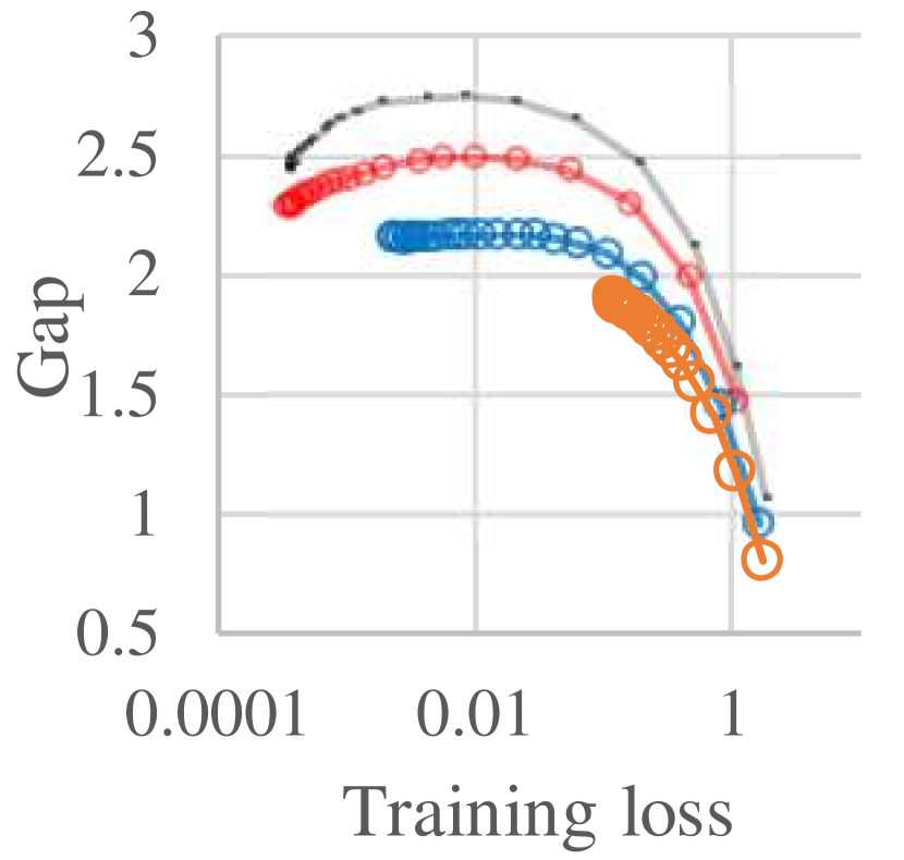
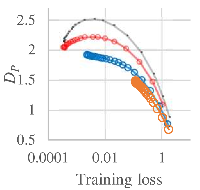
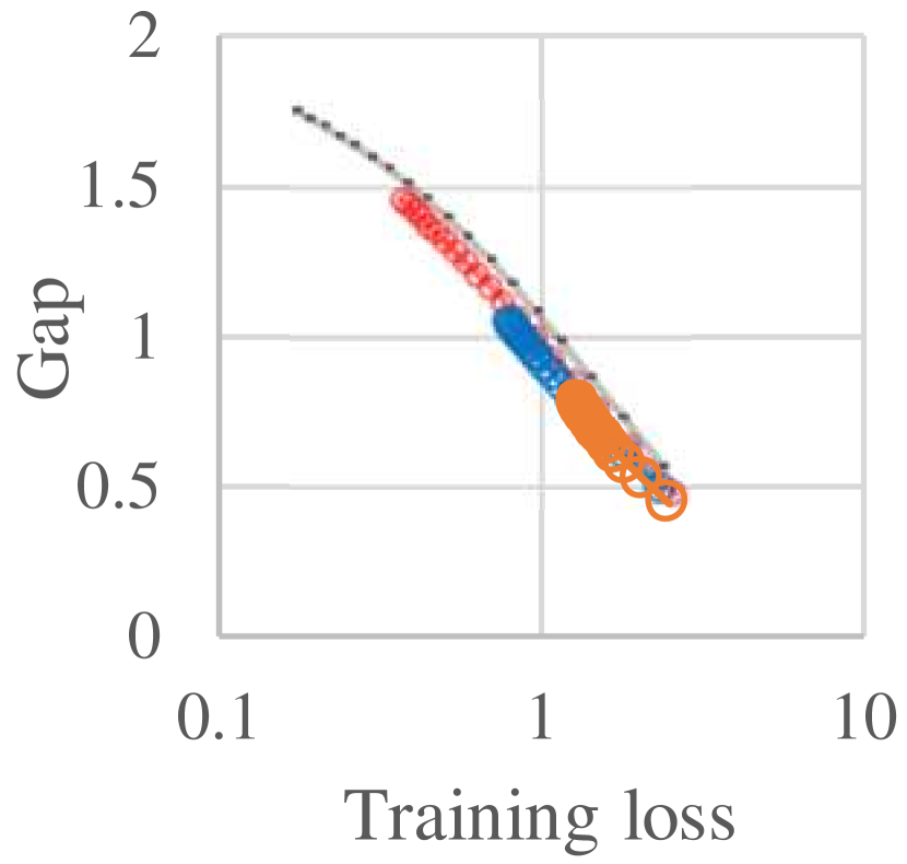
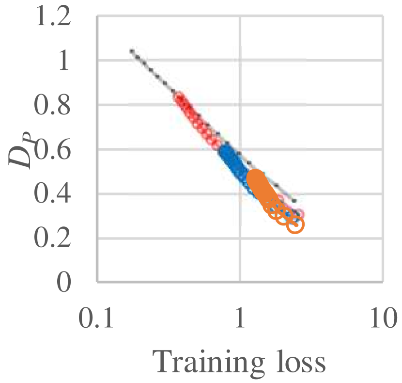
3.1.1 Results
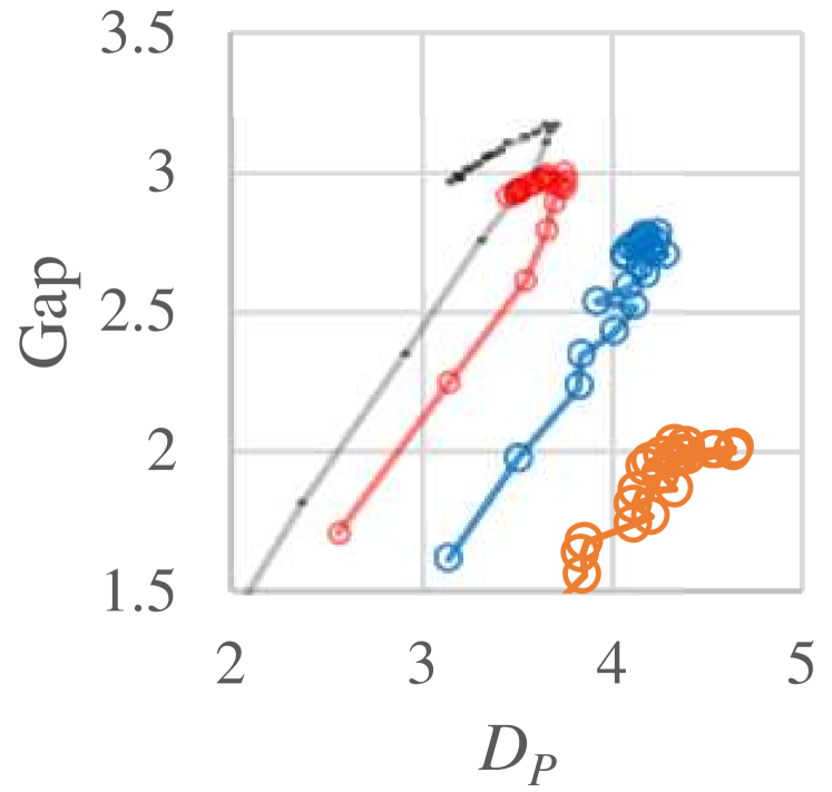
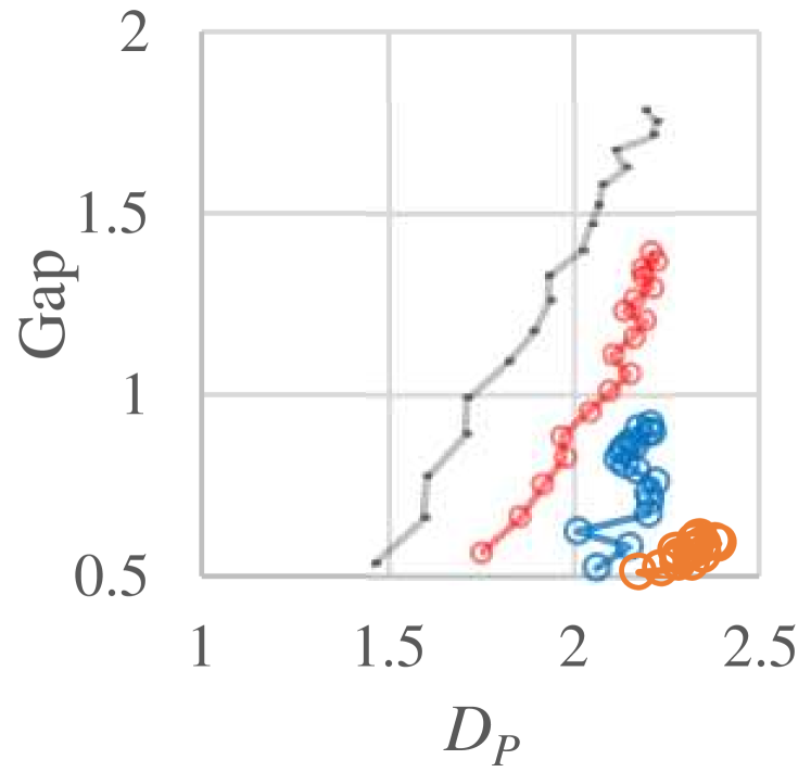
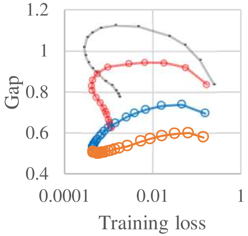
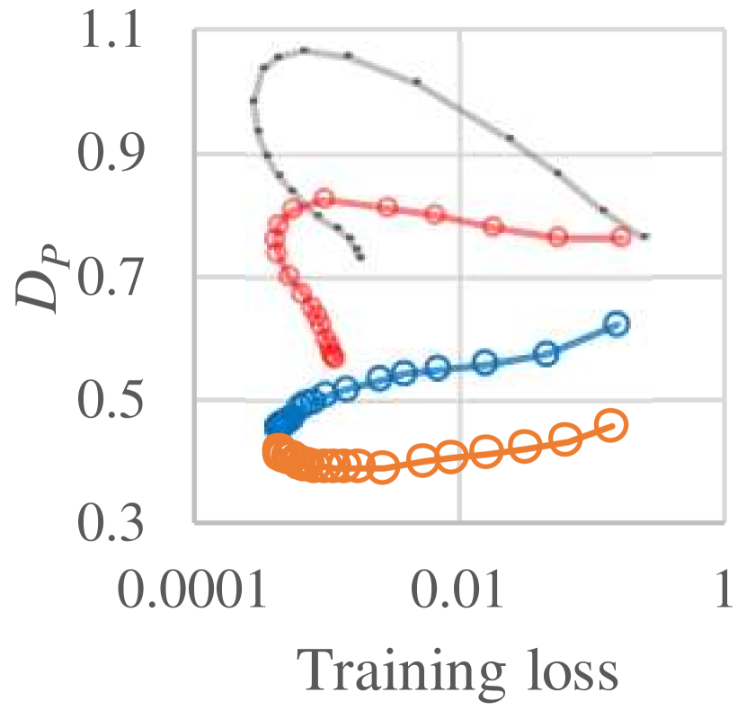
We start with the experiments that varied the learning rate and the length of training fixing anything else to see whether the change of is predictive of the change of generalization gap caused by the change of these two hyperparameters. To avoid the complex effects of learning rate decay, we trained models with SGD with a constant learning rate (constant SGD in short).
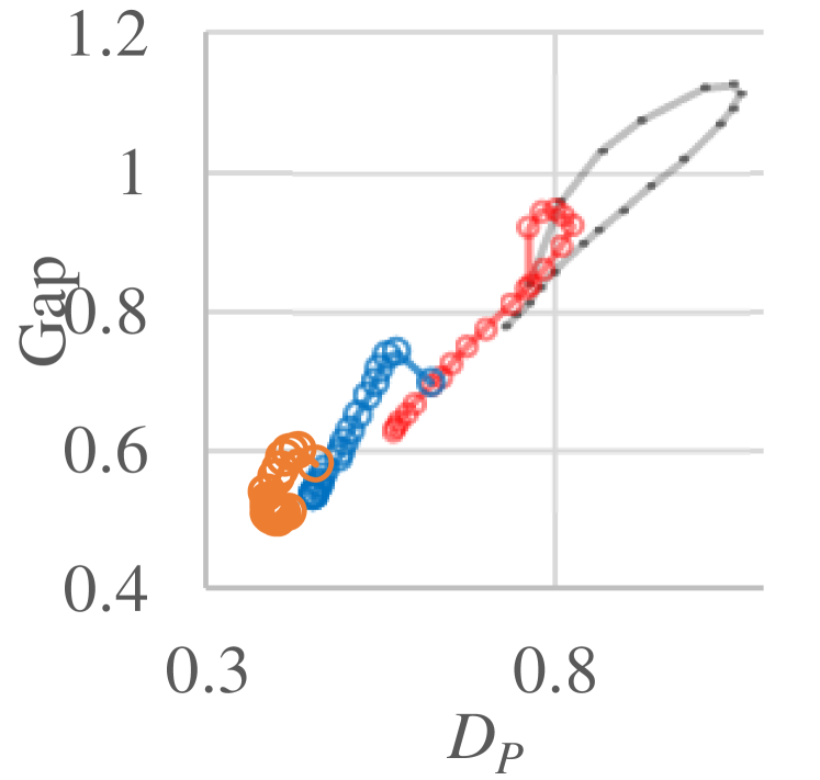
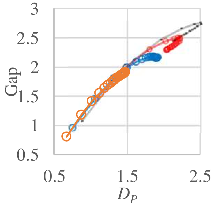
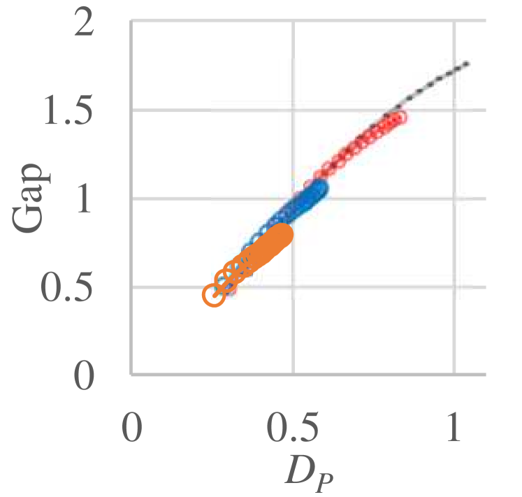
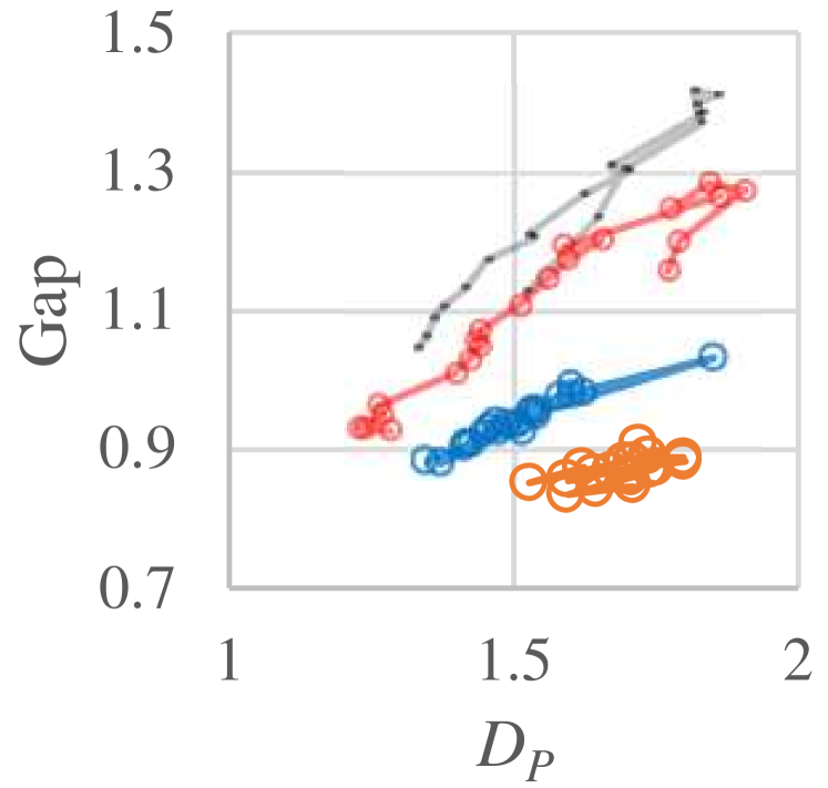
Constant SGD with iterate averaging (Fig 3,3)
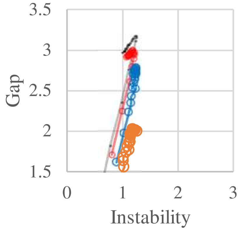
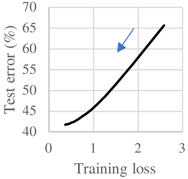
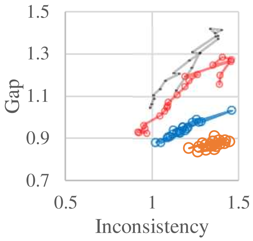
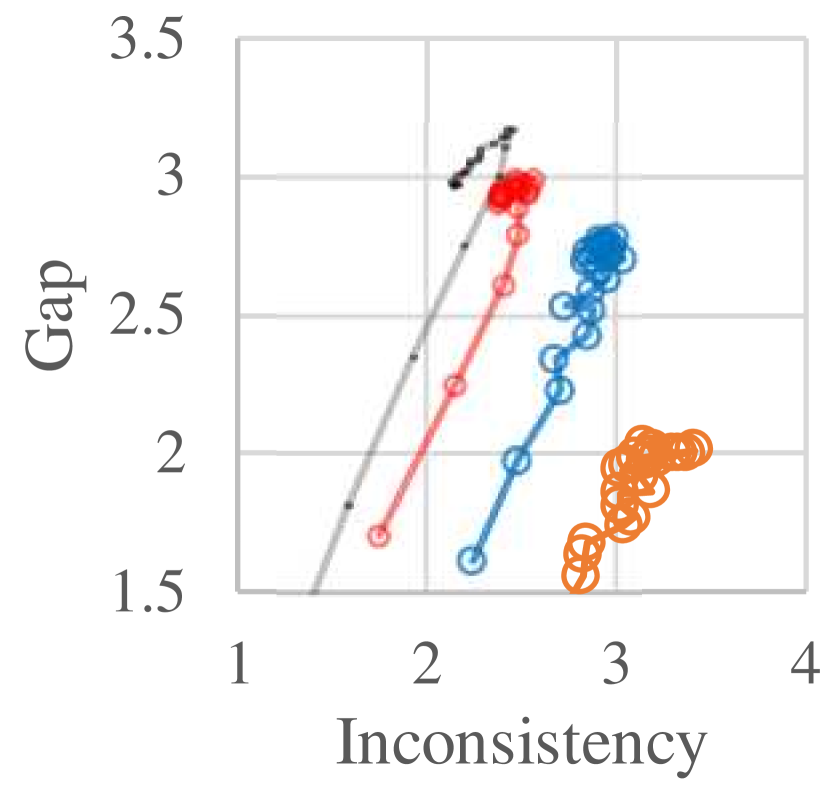
Although constant SGD could perform poorly by itself, constant SGD with iterate averaging is known to be competitive [29, 16]. Figure 3 shows (-axis) and generalization gap (-axis) of the training procedures that performed constant SGD with iterate averaging. Iterate averaging was performed by taking the exponential moving average with momentum 0.999. Each point represents a procedure (identified by the combination of the learning rate and training length), and the procedures with the same learning rate are connected by a line in the increasing order of training length. A positive correlation is observed between and generalization gap on all three datasets. Figure 3 plots generalization gap (left) and (right) on the -axis and training loss on the -axis for the same procedures as in Figure 3; observe that the up and down of is remarkably similar to the up and down of generalization gap. Also note that on CIFAR-10/100, sometimes generalization gap first goes up and then starts coming down towards the low-training-loss end of the lines (increase of training loss in some cases is due to the effects of weight decay). This ‘turning around’ of generalization gap (from going up to going down) in Figure 3 shows up as the ‘curling up’ of the upper-right end of the lines in Figure 3. It is interesting to see that and generalization gap are matching at such a detailed level.

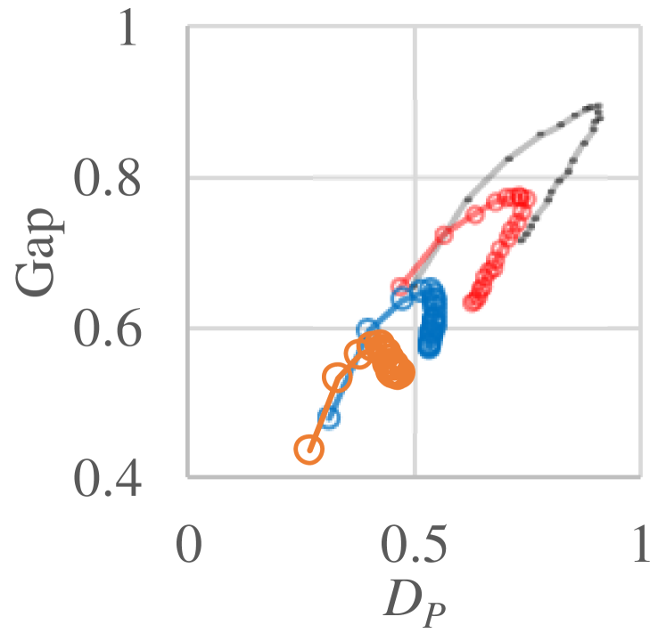
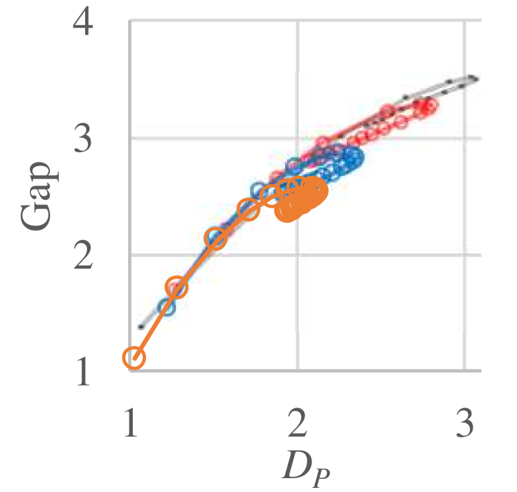
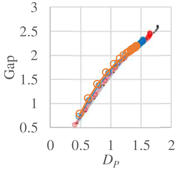
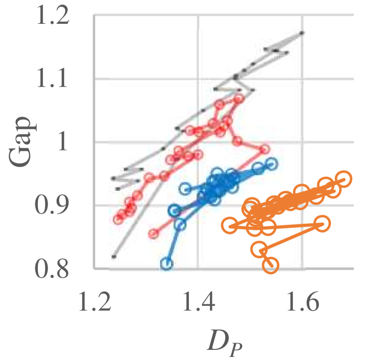
Constant SGD without iterate averaging (Fig 3,4)
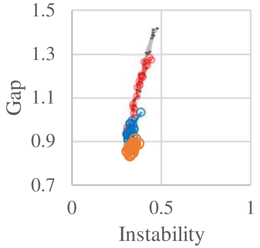
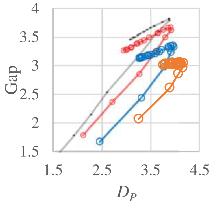
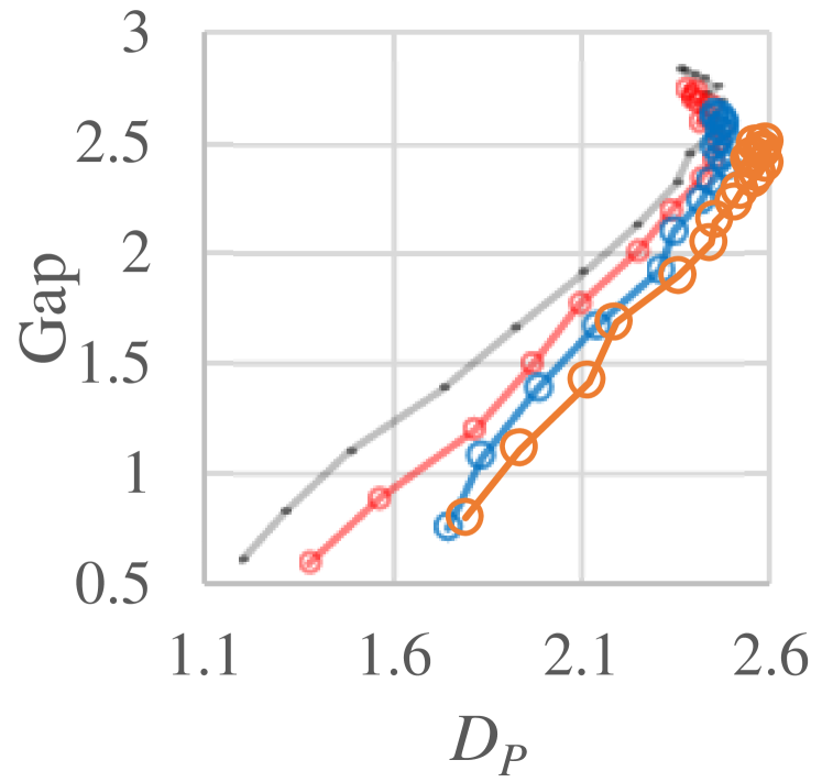
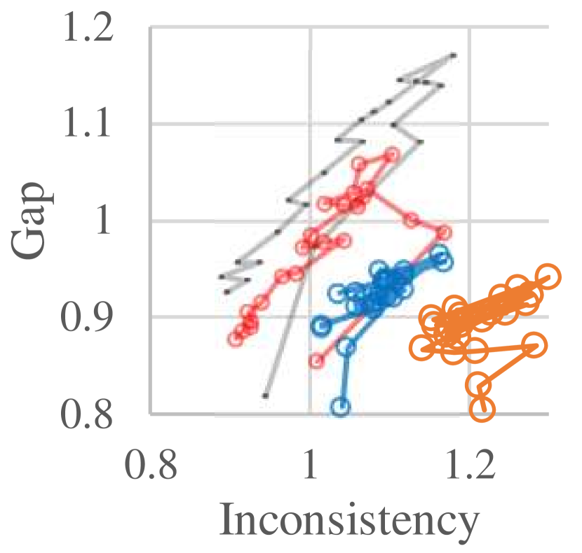
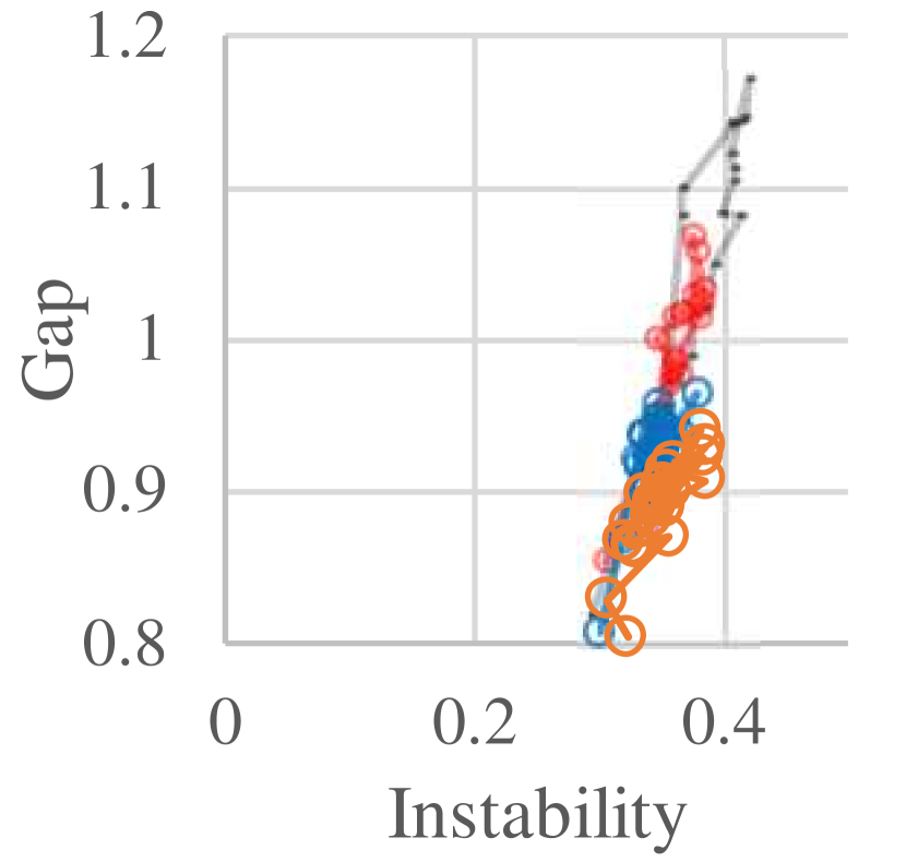
While is clearly predictive of generalization gap in the setting above, the results in Figure 3 are more complex. This figure shows (-axis) and generalization gap (-axis) for the training procedures that performed constant SGD and did not perform iterate averaging. As before, only the learning rate and training length were varied. In Figure 3, we observe that is predictive only for those which share the learning rate. For fixed generalization gap, is larger (instead of being the same) for a larger learning rate. Inspection of inconsistency and instability reveals that larger learning rates raise inconsistency although instability is mostly unaffected (see Fig 4). This is apparently the effect of high randomness/noisiness/uncertainty of the final state. As the learning rate is constant, SGD updates near the end of training bounce around the local minimum, and the random noise in the gradient of the last mini-batch has a substantial influence on the final model parameter. The influence of this noise is amplified by larger learning rates. On the other hand, is likely to be lower with higher randomness since higher randomness should make model parameter distributions flatter (less concentrated) and less dependent on the sampling of training data . This means that in this case (i.e., where the final randomness is high and varies a lot across the procedures), the interaction of and in the theoretical bound is complex, and alone could be substantially less predictive than what is indicated by the bound.
For to be predictive, final randomness should be equally low (Fig 5 (a)–(c))
Therefore, we hypothesized and empirically confirmed that for to be predictive, the degrees of final randomness/uncertainty/noisiness should be equally low, which can be achieved with either a vanishing learning rate or iterate averaging. This means that, fortunately, is mostly predictive for high-performing procedures that matter in practice.
: , : generalization gap
: Inconsistency , : generalization gap
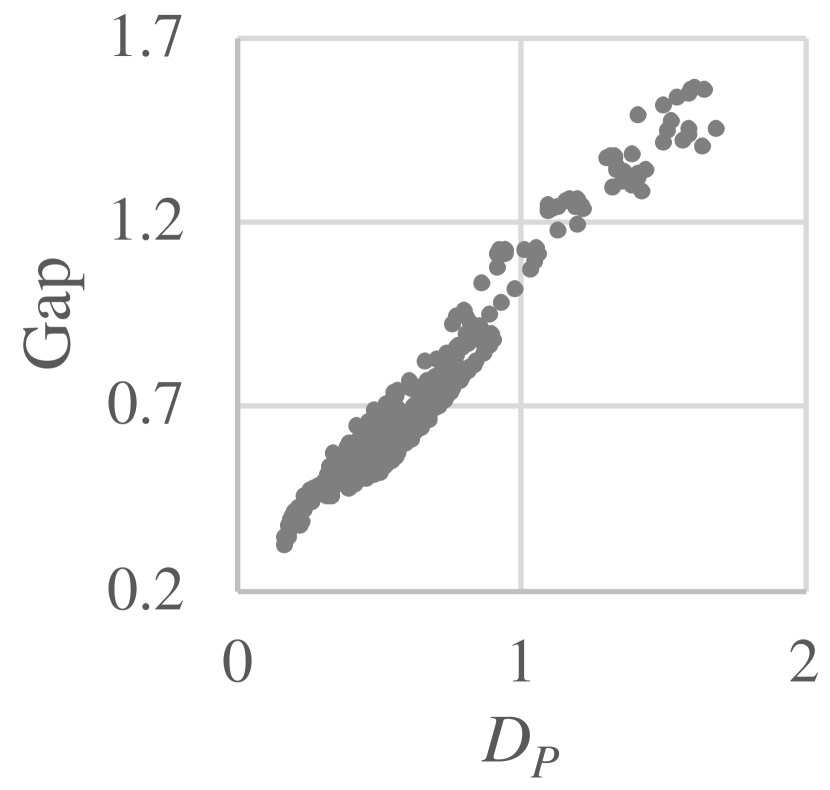
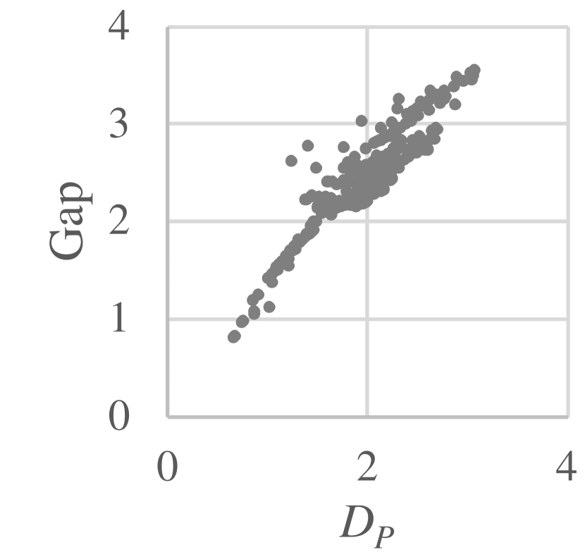
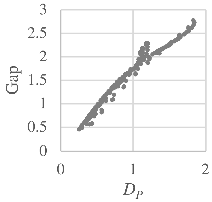
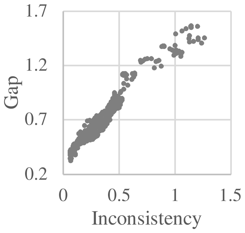
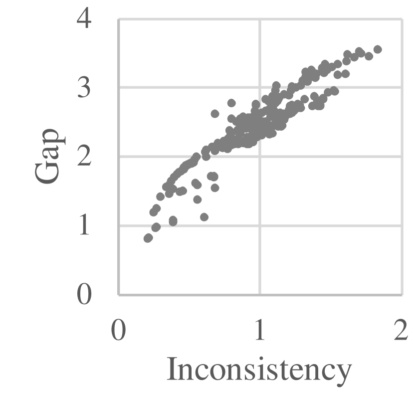
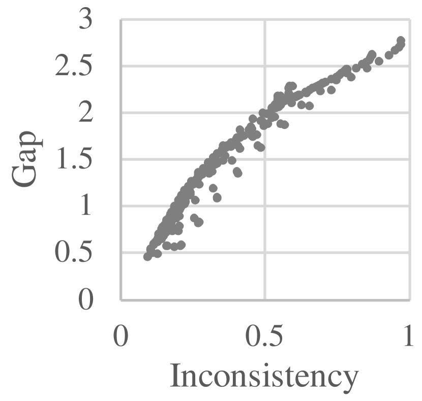
Figure 5 (a)–(c) plot (-axis) and generalization gap (-axis) for the procedures that satisfy the condition. In particular, those trained on CIFAR-10 include a wide variety of procedures that differ in network architectures, mini-batch sizes, presence/absence of data augmentation, learning rate schedules (constant or vanishing), weight decay parameters, in addition to learning rates and training lengths. A positive correlation between and generalization gap is observed on all three datasets.
Inconsistency vs. (Fig 5 (d)–(f))
Figure 5 (d)–(f) show that inconsistency is almost as predictive as when the condition of low randomness of the final states is satisfied. This is a practical advantage since unlike instability , inconsistency does not require multiple training sets for estimation.
Disagreement (Fig 7,7)
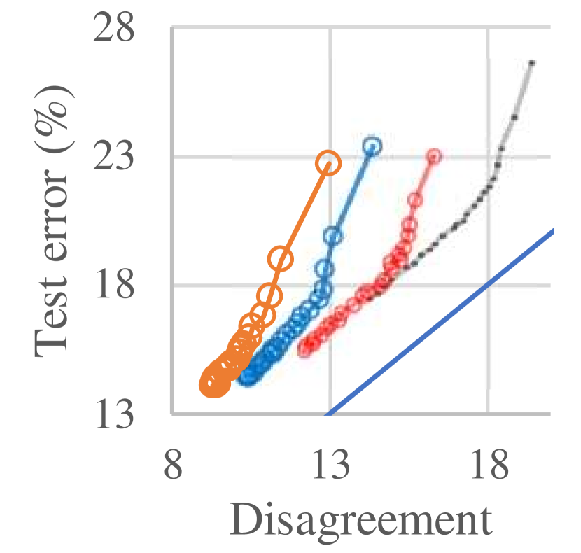
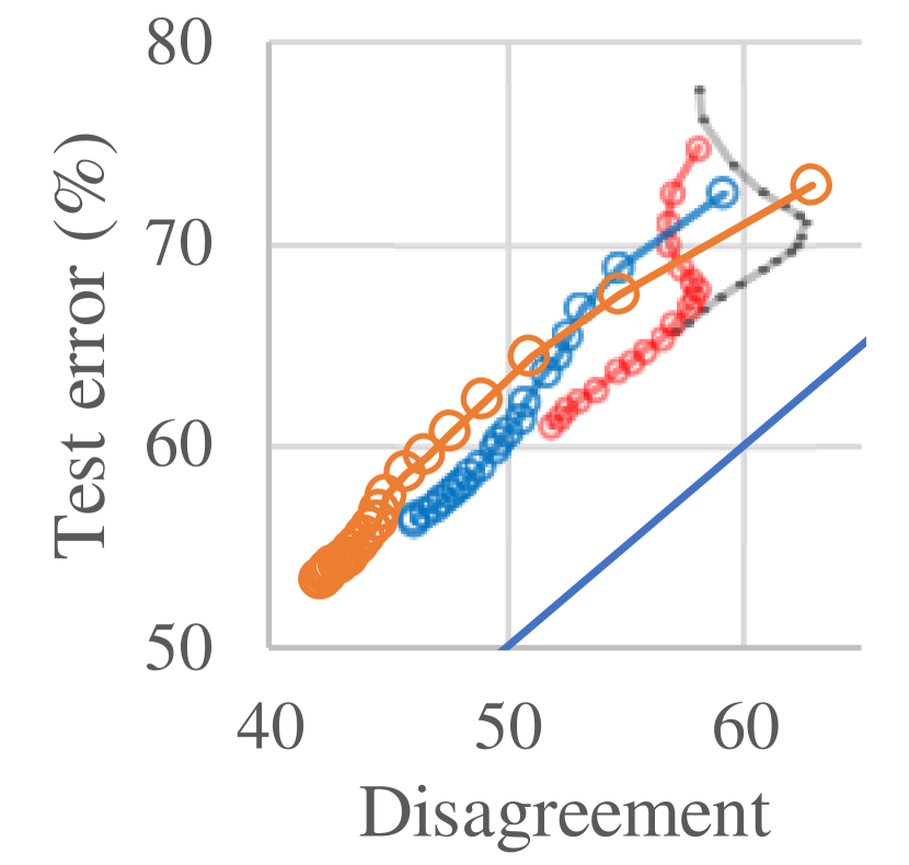
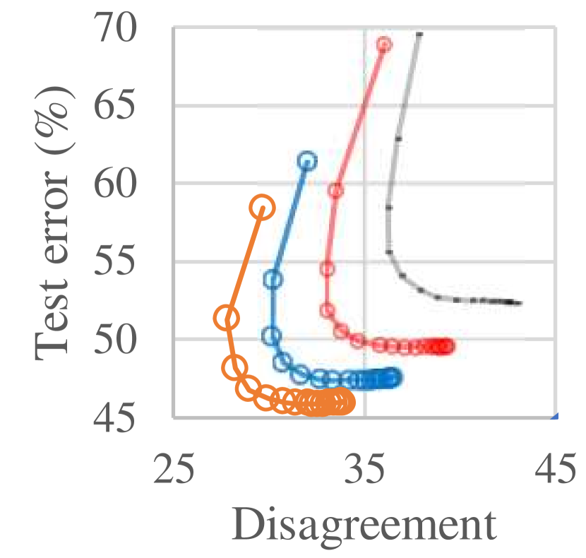
For the same procedures/models as in Figures 3 and 5, we show the relationship between disagreement and test error in Figures 7 and 7, respectively. We chose test error instead of generalization gap for the -axis since the previous finding was ‘Disagreement Test error’. The straight lines are . The relation in Fig 7 (a) and Fig 7 (a) is close to equality, but the relation appears to be more complex in the others. The procedures plotted in Fig 7 are those which satisfy the condition for to be predictive of generalization gap; thus, the results indicate that the condition for disagreement to be predictive of test error is apparently different.
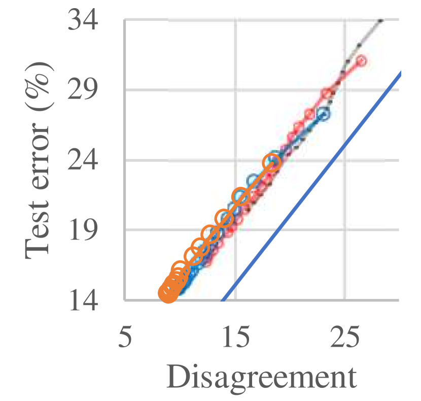
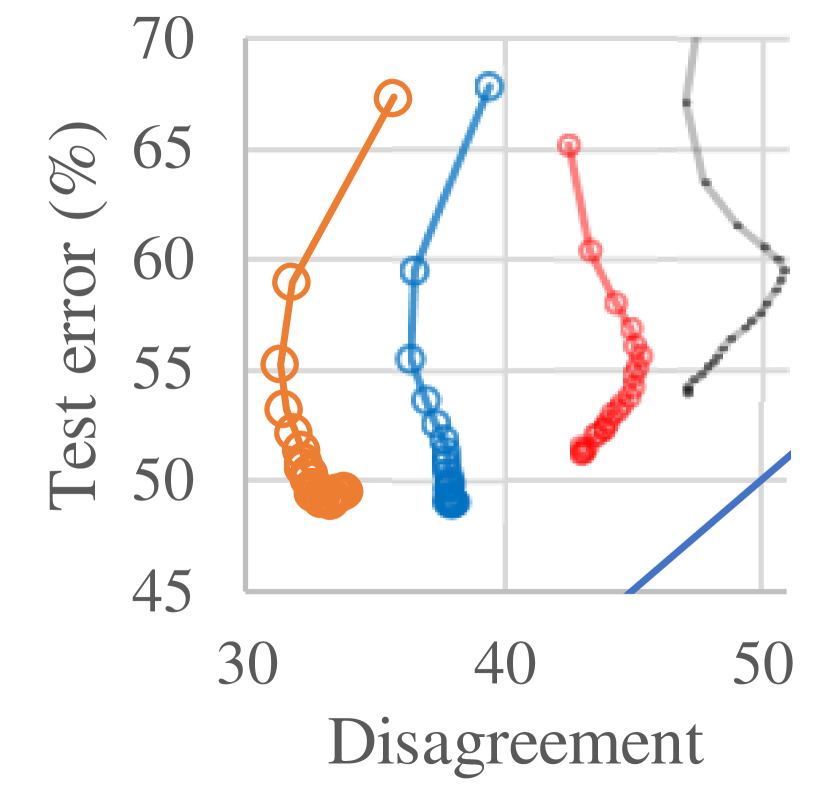
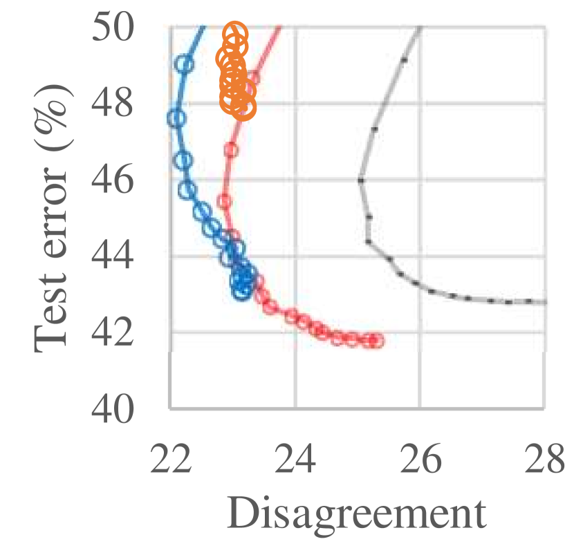
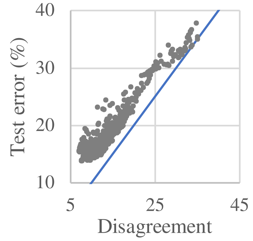
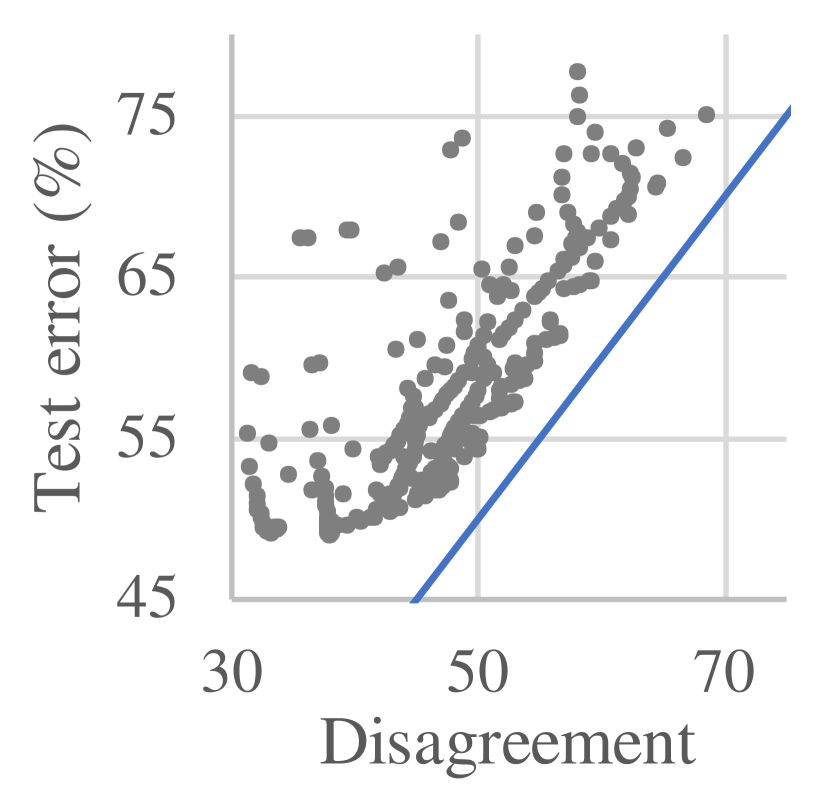
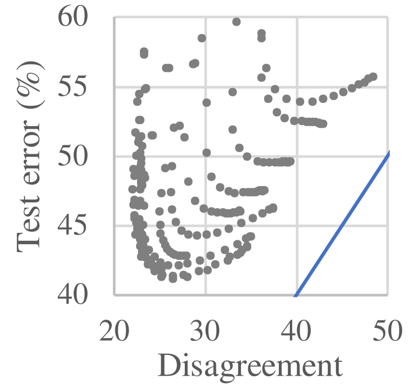
Note that while the previous empirical study of disagreement [27, 17] focused on the models with zero training error, we studied a wider range of models. Unlike CIFAR-10/100 (on which zero training error can be quickly achieved), a common practice for datasets like ImageNet is budgeted training [25] instead of training to zero error. Also note that zero training error does not necessarily lead to the best performance, which, for example, has been observed in the ImageNet experiments of this section.
3.2 On the predictiveness of inconsistency : from an algorithmic perspective
Based on the results above, this section focuses on inconsistency , which enables experiments with larger training data, and studies the behavior of inconsistency in comparison with sharpness from an algorithmic perspective.
Training objectives
Parallel to the fact that SAM seeks flatness of training loss landscape, a meta-algorithm co-distillation (named by [1], and closely related to deep mutual learning [42], summarized in Algorithm 1 in the Appendix) encourages consistency of model outputs. It simultaneously trains two (or more) models with two (or more) different random sequences while penalizing the inconsistency between the predictions of the two models. This is typically described as ‘teaching each other’, but we take a different view of consistency encouragement. Note that the penalty term merely ‘encourages’ low inconsistency. Since inconsistency by definition depends on the unknown data distribution, it cannot be directly minimized by training. The situation is similar to minimizing loss on the training data with the hope that loss will be small on unseen data. We analyzed the models that were trained with one of the following training objectives (shown with the abbreviations used below):
-
•
‘Standard’: the standard cross-entropy loss.
-
•
‘Consist.’: the standard loss with encouragement of consistency.
-
•
‘Flat.’: the SAM objective, which encourages flatness.
-
•
‘Consist+Flat’: encouraging both consistency and flatness. Coupling two instances of SAM training with the inconsistency penalty term.
Cases
We experimented with ten combinations (cases) of dataset, network architecture, and training scenario. Within each case, we fixed the basic settings (e.g., weight decay, learning rate) to the ones known to perform well from the previous studies, and only varied the training objectives so that for each case we had at least four stochastic training procedures distinguished by the four training objectives (for some cases, we had more than four due to testing multiple values of for SAM). We obtained four models (trained with four different random sequences) per training procedure. Tables 2 and 2 show the datasets and network architectures we used, respectively. Note that as a result of adopting high-performing settings, all the cases satisfy the condition of low final randomness.
| Name | #class | #train | #dev | #test | |
|---|---|---|---|---|---|
| provided | used | ||||
| ImageNet [7] | 1000 | 1.28M | 1.27M | 10K | 50K |
| Food101 [3] | 101 | 75750 | 70700 | 5050 | 25250 |
| Dogs [21] | 120 | 12000 | 10800 | 1200 | 8580 |
| Cars [23] | 196 | 8144 | 7144 | 1000 | 8041 |
| CIFAR-10 [24] | 10 | 50000 | 4000 | 5000 | 10000 |
| MNLI [36] | 3 | 392702 | 382902 | 9800 | 9815 |
| QNLI [36] | 2 | 104743 | 99243 | 5500 | 5463 |
3.2.1 Results
As in the previous section, we quantify the generalization gap by the difference of test loss from training loss (note that the loss is the cross-entropy loss; the inconsistency penalty or anything else is not included); the inconsistency values were again measured on the held-out unseen unlabeled data, disjoint from both training data and test data. Two types of sharpness values were measured, 1-sharpness (per-example loss difference in the adversarial direction) of [10] and the magnitude of the loss Hessian (measured by the largest eigenvalue), which represent the sharpness of training loss landscape and have been shown to correlate to generalization performance [10].

Food101 ViT-B16, from scratch
MNLI, fine-tuning of RoBERTa-base


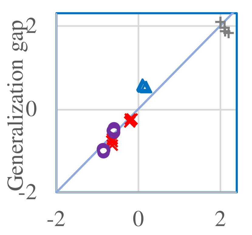
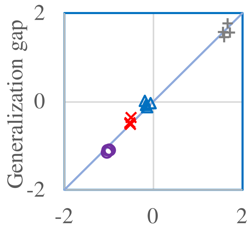
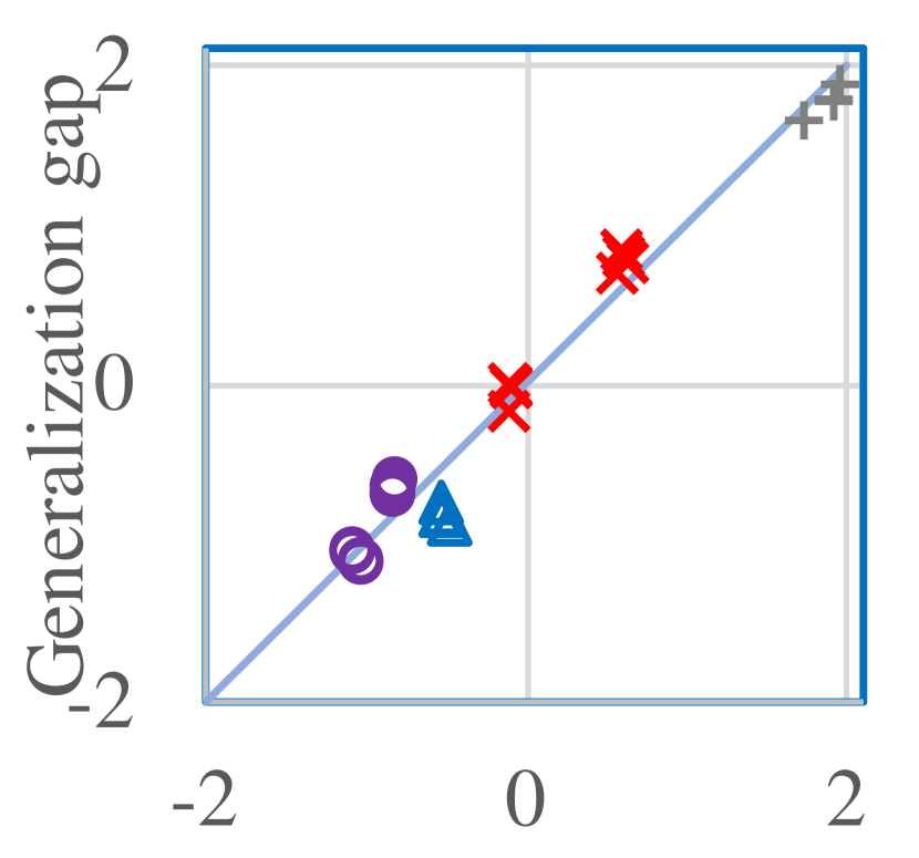
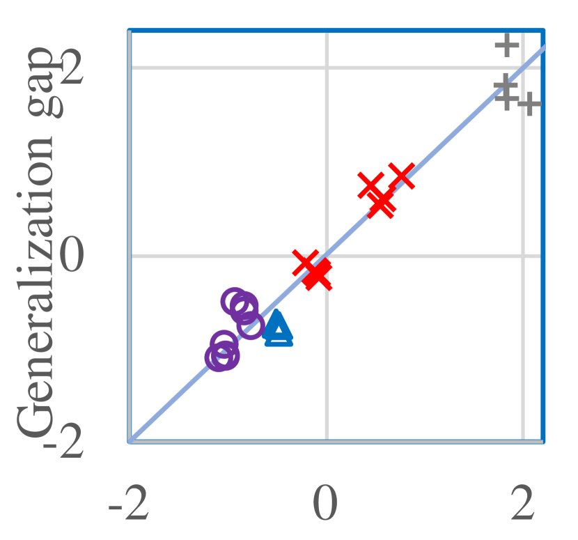
Inconsistency correlates to generalization gap (Figure 8)
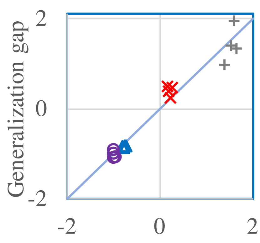
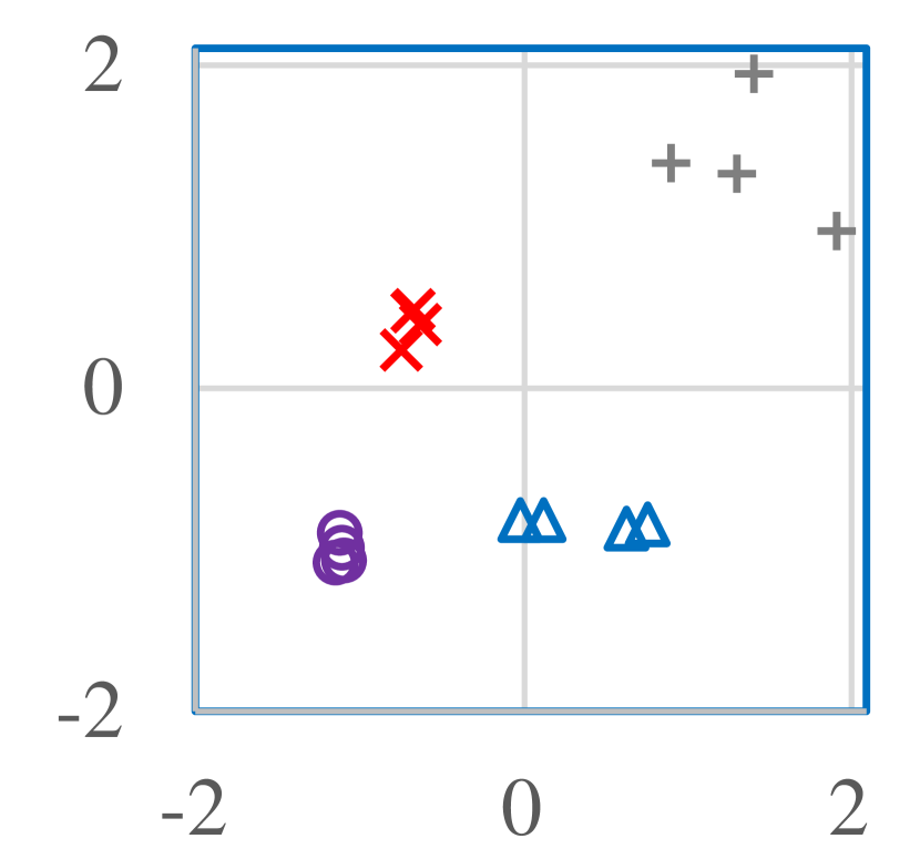
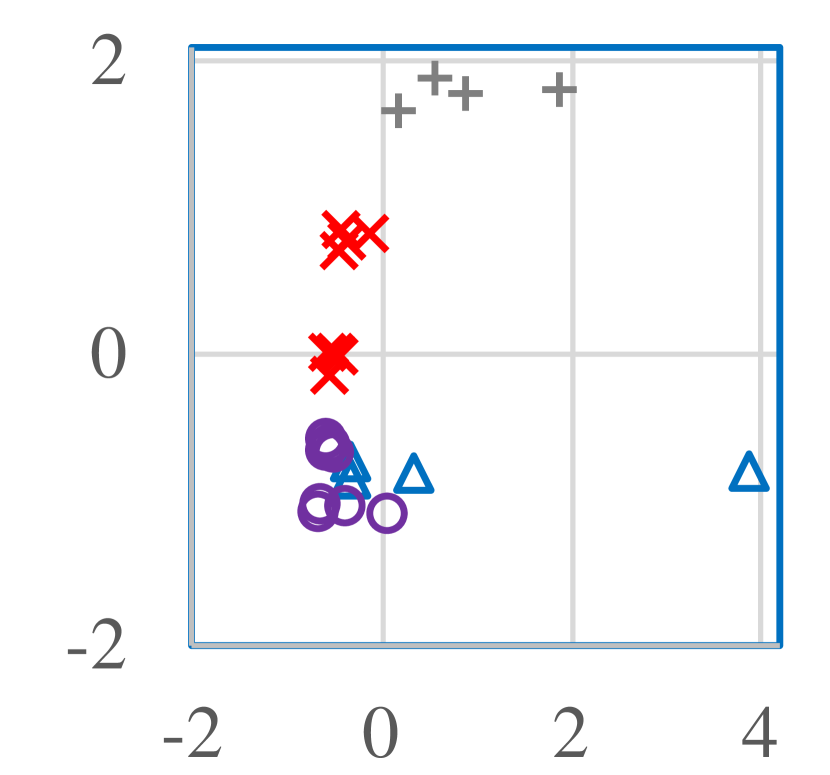
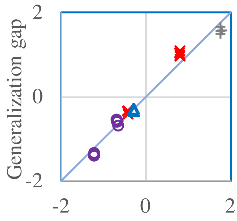
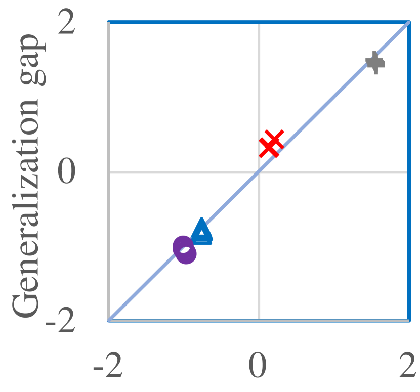
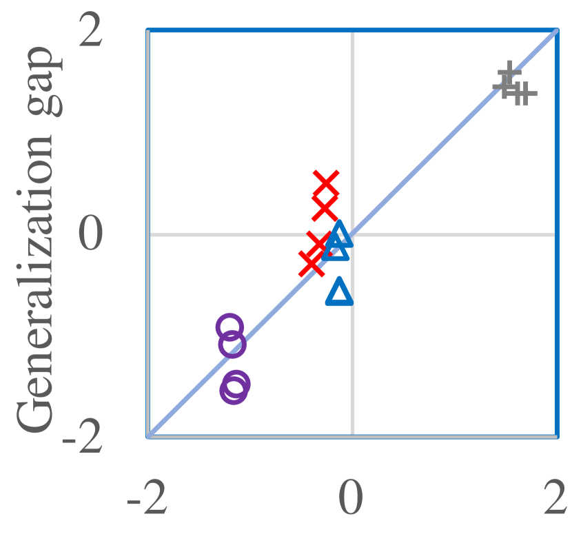
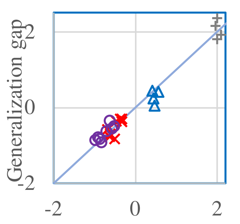
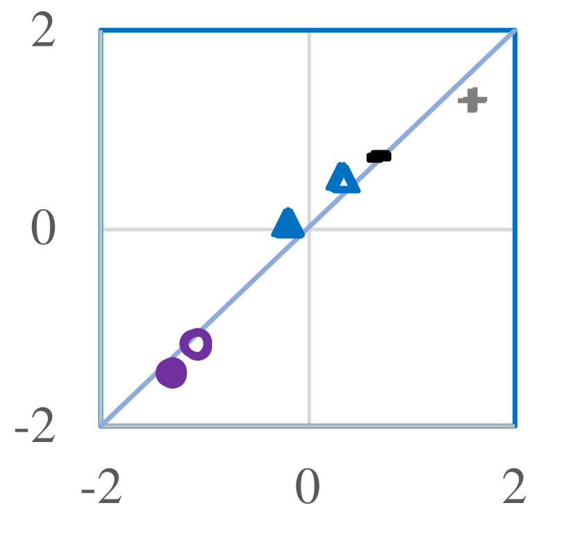
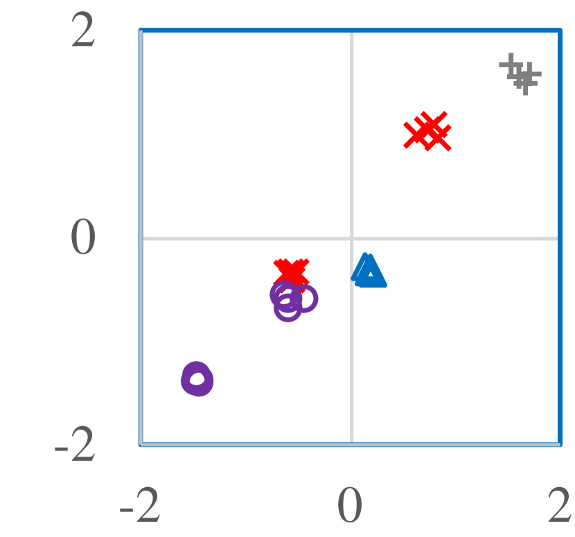
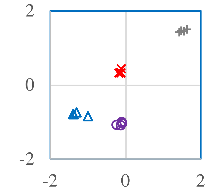
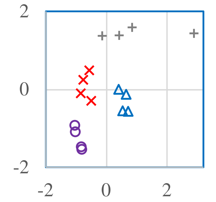
Figure 8 shows inconsistency or sharpness values (-axis) and the generalization gap (-axis). Each point in the figures represents a model; i.e., in this section, we show model-wise quantities (instead of procedure-wise), simulating the model selection setting. (Model-wise inconsistency for model trained on with procedure is .) All quantities are standardized so that the mean is zero and the standard deviation is 1. In the figures, we distinguish the four training objectives. In Figure 8 (b) and (c), we confirm, by comparing the ‘Flat.’ models () with the baseline standard models (), that encouragement of flatness (by SAM) indeed reduces sharpness (-axis) as well as the generalization gap (-axis). This serves as a sanity check of our setup.
We observe in Figure 8 that inconsistency shows a clear positive correlation with the generalization gap, but the correlation of sharpness with generalization gap is less clear (e.g., in (b)–(c), the generalization gap of the ‘Consist.’ models () is much smaller than that of the ‘Flat.’ models (), but their sharpness is larger). This is a general trend observed across multiple network architectures (ResNet, Transformers, MLP-Mixer, and so on), multiple datasets (images and texts), and multiple training scenarios (from scratch, fine-tuning, and distillation); the Appendix provides the figures for all 10 cases. Moreover, we found that while both sharpness reduction and inconsistency reduction lead to better generalization, in a number of cases inconsistency and generalization gap are reduced and yet sharpness remains relatively high. We view this phenomenon as an indication that inconsistency has a stronger (and perhaps more essential) connection with generalization gap than sharpness.
Inconsistency is more predictive of generalization gap than sharpness (Table 3)
Motivated by the linearity observed in the figure above, we define a linear predictor of the generalization gap that takes the inconsistency or sharpness value as input. We measure the predictive power of the metrics through the prediction performance of this linear predictor trained with least square minimization. To make the inconsistency and sharpness values comparable, we standardize them and also generalization gap. For each case, we evaluated the metrics by performing the leave-one-out cross validation on the given set of models (i.e., perform least squares using all models but one and evaluate the obtained linear predictor on the left-out model; do this times for models and take the average). The results in Table 3 show that inconsistency outperforms sharpness, and the superiority still generally holds even when sharpness is given an ‘unfair’ advantage of additional labeled data.
| Case# | 1 | 2 | 3 | 4 | 5 | 6 | 7 | 8 | 9 | 10 |
|---|---|---|---|---|---|---|---|---|---|---|
| Dataset | ImageNet | Food101 | C10 | Dog | Car | Mnli | Qnli | Food | ||
| Training scenario | From scratch | Fine-tuning | Distill. | |||||||
| Inconsistency | 0.13 | 0.10 | 0.17 | 0.27 | 0.15 | 0.09 | 0.19 | 0.15 | 0.18 | 0.19 |
| 1-sharpness | 0.21 | 0.48 | 0.75 | 0.74 | 0.84 | 0.34 | 0.24 | 0.58 | 0.98 | 0.75 |
| Hessian | 0.50 | 1.00 | 0.77 | 0.72 | 0.78 | 0.70 | 0.68 | 0.59 | 0.87 | 0.59 |
| Giving the sharpness metrics an ‘unfair’ advantage by providing additional labels: | ||||||||||
| 1-sharpness of dev. loss | 0.14 | 0.64 | 0.47 | 0.40 | 0.72 | 0.22 | 0.14 | 0.36 | 0.37 | 0.62 |
| Hessian of dev. loss | 0.45 | 0.82 | 0.58 | 0.75 | 0.13 | 0.27 | 0.15 | 0.91 | 0.81 | 0.89 |
3.3 Practical impact: algorithmic consequences
The results above suggest a strong connection of inconsistency of model outputs with generalization, which also suggests the importance of seeking consistency in the algorithmic design. To confirm this point, we first experimented with two methods (ensemble and distillation) and found that in both, encouraging low inconsistency in every stage led to the best test error. Note that in this section we report test error instead of generalization gap in order to show the practical impact.
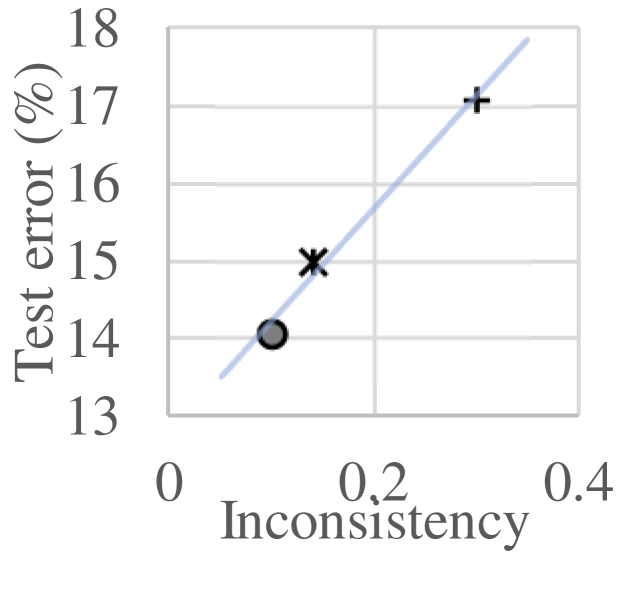

(a) Ensemble reduces inconsistency (-axis) and test error (-axis). Non-ensemble (baseline), Ensemble of standard models, Ensemble of the models trained with consistency encouragement. RN18 on Food101.
(b) Test error (-axis) and inconsistency of distilled models (-axis). Without unlabeled data. No distillation, △ Standard distillation, Consistency encouragement for the student, Consistency encouragement for both the student and teacher. The best performance is obtained when consistency is encouraged for both the teacher and student. Food101. Student: RN18, Teacher: RN18 (left), RN50 (middle), and fine-tuning of ImageNet-trained ENB0 (right). In both (a) and (b), the average of 4 models is shown; see Appendix for the standard deviations.
Ensemble (Fig 9 (a))
Figure 9 (a) shows that, compared with non-ensemble models (), ensemble models (averaging logits of two models) reduce both inconsistency (-axis) and test error (-axis). It is intuitive that averaging the logits would cancel out the dependency on (or particularities of) the individual random sequences inherent in each single model; thus, outputs of ensemble models are expected to become similar and so consistent (as empirically observed). Moreover, we presume that reduction of inconsistency is the mechanism that enables ensemble to achieve better generalization. The best test error was achieved when the ensemble was made by two models trained with consistency encouragement ( in Fig 9 (a)).
Distillation (Fig 9 (b))
We experimented with distillation [13] with encouragement of consistency for the teacher model and/or the student model. Figure 9 (b) shows the test error (-axis) and the inconsistency (-axis). The standard model () serves as the baseline. The knowledge level of teachers increases from left to right, and within each graph, when/whether to encourage consistency differs from the point to point. The main finding here is that at all the knowledge levels of the teacher, both inconsistency and test error go down as the pursuit of consistency becomes more extensive; in each graph, the points for the distilled models form a nearly straight line. (The line appears to shift away from the baseline () as the amount of external knowledge of the teacher increases. We conjecture this could be due to the change in .) While distillation alone reduces inconsistency and test error, the best results are obtained by encouraging consistency at every stage of training (i.e., training both the teacher and student with consistency encouragement). The results underscore the importance of inconsistency reduction for better performance.
On the pursuit of the state of the art (Table 5,5)
We show two examples of obtaining further improvement of state-of-the-art results by adding consistency encouragement. The first example is semi-supervised learning with CIFAR-10. Table 5 shows that the performance of a state-of-the-art semi-supervised method can be further improved by encouraging consistency between two training instances of this method on the unlabeled data (Algorithm 2 in the Appendix). The second example is transfer learning. We fine-tuned a public ImageNet-trained EfficientNet with a more focused dataset Food101. Table 5 shows that encouraging consistency between two instances of SAM training improved test error. These examples demonstrate the importance of consistency encouragement in the pursuit of the state of the art performance.
| Methods | Error (%) | |
| Copied | MixMatch [2] | 6.42 |
| from [32] | UDA [37] | 4.88 |
| FixMatch [32] | 4.26 | |
| Our results | FixMatch | 4.25±0.15 |
| UDA (no sharpening) | 4.33±0.10 | |
| UDA + ‘Consist.’ | 3.95±0.12 | |
| RandAugment [6] was used for UDA and FixMatch. | ||
| Methods | Error (%) | |
| Previous | EN-B4 [33] | 8.5 |
| results | EN-B7 [10] | 7.17 |
| EN-B7 SAM [10] | 7.02 | |
| Our results | EN-B4 SAM | 6.00±0.05 |
| EN-B4 SAM + ‘Consist.’ | 5.77±0.04 | |
| The improvement over EN-B7 SAM of [10] is due to the difference in the basic setting; see Appendix. | ||
4 Limitations and discussion
Theorem 2.1 assumes a bounded loss though the standard loss for classification is the cross-entropy loss, which is unbounded. This assumption can be removed by extending the theorem to a more complex analysis with other moderate assumptions. We, however, chose to present the simpler and so more intuitive analysis with a bounded loss. As noted above, this theorem is intended for stochastic training procedures. The bound may not be useful for deterministic procedures, and this characteristics is not unique to our analysis but shared by the previous information-theoretic analysis of stochastic machine learning algorithms [38, 30, 28].
We acknowledge that due to resource constraints, there was a limitation to the diversity of the training procedures we empirically analyzed. In particular, our study of inconsistency and instability in Section 3.1 started with simpler cases of constant learning rate SGD and later included the cases of learning rate decay (Figure 5); consequently, the types of the training procedures studied in Section 3.1 were skewed towards the constant learning rate SGD. The models analyzed in Figure 5 were less diverse with CIFAR-100 and ImageNet than with CIFAR-10, as noted above, and again this asymmetry was due to the resource constraints. On the other hand, the models analyzed in this work are in a sense more diverse than the previous empirical studies [27, 17] of the disagreement metric (related to our inconsistency), which were restricted to the models with near zero train error.
In Section 3.2, we studied inconsistency from the algorithmic perspective in comparison with the sharpness metrics. We chose sharpness for comparison due to its known correlation to generalization performance and the existence of the algorithm (SAM) to reduce it. We acknowledge that there can be other metrics that are predictive of generalization gap.
Although the correlation of the disagreement metric with generalization gap is relatively poor in the settings of Section 3.1 (e.g., Figure 10), it is plausible that disagreement can be as predictive of generalization gap as inconsistency in some settings, for example, when the confidence level of predictions is sufficiently high since in that case, Theorem 2.1 should provide a theoretical basis also for disagreement though indirectly (details are provided in Appendix D.3). Moreover, for improving stochastic training of deep neural networks, it would be useful to understand the connection between generalization performance and discrepancies of model outputs in general (whether instability, inconsistency, disagreement, or something else), and we hope that this work contributes to pushing forward in this direction.
5 Conclusion
We presented a theory that relates generalization gap to instability and inconsistency of model outputs, which can be estimated on unlabeled data, and empirically showed that they are strongly predictive of generalization gap in various settings. In particular, inconsistency was shown to be a more reliable indicator of generalization gap than commonly used local flatness. We showed that algorithmic encouragement of consistency reduces inconsistency as well as test error, which can lead to further improvement of the state of art performance. Finally, our results provide a theoretical basis for existing methods such as co-distillation and ensemble.
References
- [1] Rohan Anil, Gabriel Pereyra, Alexandre Passos, Robert Ormandi, George E. Dahl, and Geoffrey E. Hinton. Large scale distributed neural network training through online distillation. In International Conference on Learning Representations (ICLR), 2018.
- [2] David Berthelot, Nicholas Carlini, Ian Goodfellow, Nicolas Papernot, Avital Oliver, and Colin Raffel. MixMatch: A holistic approach to semi-supervised learning. In Proceedings of the 36th International Conference on Machine Learning (ICML), 2019.
- [3] Lukas Bossard, Matthieu Guillaumin, and Luc Van Gool. Food-101 – mining discriminative components with random forests. In European Conference on Computer Vision, 2014.
- [4] Olivier Bousquet and André Elisseef. Stability and generalization. Journal of Machine Learning Research, 2:499–526, 2002.
- [5] Xiangning Chen, Cho-Jui Hsieh, and Boqing Gong. When vision transformers outperform resnets without pre-training or strong data augmentations. In International Conference on Learning Representations (ICLR), 2022.
- [6] Ekin D. Cubuk, Barret Zoph, Jonathon Shlens, and Quoc V. Le. RandAugment: Practical automated data augmentation with a reduced search space. In Advances in Neural Information Processing Systems 33 (NeurIPS 2020), 2020.
- [7] Jia Deng, Wei Dong, Richard Socher, Li-Jia Li, Kai Li, and Li Fei-Fei. ImageNet: A large-scale hierarchical image database. In Proceedings of the IEEE Conference on Computer Vision and Pattern Recognition (CVPR), 2009.
- [8] Terrance DeVries and Graham W. Taylor. Improved regularization of convolutional neural networks with cutout. arXiv:1708.04552, 2017.
- [9] Alexey Dosovitskiy, Lucas Beyer, Alexander Kolesnikov, Dirk Weissenborn, Xiaohua Zhai, Thomas Unterthiner, Mostafa Dehghani, Matthias Minderer, Georg Heigold, Sylvain Gelly, Jakob Uszkoreit, and Neil Houlsby. An image is worth 16x16 words: Transformers for image recognition at scale. In International Conference on Learning Representations (ICLR), 2021.
- [10] Pierre Foret, Ariel Kleiner, Hossein Mobahi, and Behnam Neyshabur. Sharpness-aware minimization for efficiently improving generalization. In International Conference on Learning Representations (ICLR), 2021.
- [11] Xavier Gastaldi. Shake-shake regularization. arXiv:1705.07485, 2017.
- [12] Kaiming He, Xiangyu Zhang, Shaoqing Ren, and Jian Sun. Deep residual learning for image recognition. In Proceedings of the IEEE Conference on Computer Vision and Pattern Recognition (CVPR), 2016.
- [13] Geoffrey Hinton, Oriol Vinyals, and Jeff Dean. Distilling the knowledge in a neural network. In Proceedings of Deep Learning and Representation Learning Workshop: NIPS 2014, 2014.
- [14] Sepp Hochreiter and Jürgen Schmidhuber. Flat minima. Neural Computation, 9:1–42, 1997.
- [15] Gao Huang, Yu Sun, Zhuang Liu, Daniel Sedra, and Kilian Weinberger. Deep networks with stochastic depth. In Proceedings of European Conference on Computer Vision (ECCV), 2016.
- [16] Pavel Izmailov, Dmitrii Podoprikhin, Timur Garipov, Dmitry Vetrov, and Andrew Gordon Wilson. Averaging weights leads to wider optima and better generalization. In Proceedings of the Conference on Uncertainty in Artificial Intelligence (UAI), 2018.
- [17] Yiding Jiang, Vaishnavh Nagarajan, Christina Baek, and J. Zico Kolter. Assessing generalization of SGD via disagreement. In International Conference on Learning Representations (ICLR), 2022.
- [18] Yiding Jiang, Behnam Neyshabur, Hossein Mobahi, Dilip Krishnan, and Samy Bengio. Fantastic generalization measures and where to find them. In International Conference on Learning Representations (ICLR), 2020.
- [19] Rie Johnson and Tong Zhang. Guided learning of nonconvex models through successive functional gradient optimization. In Proceedings of the 37th International Conference on Machine Learning (ICML), 2020.
- [20] Nitish Shirish Keskar, Dheevatsa Mudigere, Jorge Nocedal, Mikhail Smelyanskiy, and Ping Tak Peter Tang. On large-batch training for deep learning: Generalization gap and sharp minima. In International Conference on Learning Representations (ICLR), 2017.
- [21] Aditya Khosla, Nityananda Jayadevaprakash, Bangpeng Yao, and Li Fei-Fei. Novel dataset for fine-grained image categorization. In First Workshop on Fine-Grained Visual Categorization, IEEE Conference on Computer Vision and Pattern Recognition (CVPR), 2011.
- [22] Andreas Kirsch and Yarin Gal. A note on “Assessing generalization of SGD via disagreement”. Transactions on Machine Learning Research, 2022.
- [23] Jonathan Krause, Michael Stark, Jia Deng, and Li Fei-Fei. 3D object representations for fine-grained categorization. In 4th International IEEE Workshop on 3D Representation and Recognition (3dRR-13), Sydney, Australia, 2013.
- [24] Alex Krizhevsky. Learning multiple layers of features from tiny images. Technical report, 2009.
- [25] Mengtian Li, Ersin Yumer, and Deva Ramanan. Budgeted training: Rethinking deep neural network training under resource constraints. In International Conference on Learning Representations (ICLR), 2020.
- [26] Yinhan Liu, Myle Ott, Naman Goyal, Jingfei Du, Mandar Joshi, Danqi Chen, Omer Levy, Mike Lewis, Luke Zettlemoyer, and Veselin Stoyanov. RoBERTa: A robustly optimized BERT pretraining approach. arXiv:1907.11692, 2019.
- [27] Preetum Nakkiran and Yamini Bansal. Distributional generalization: A new kind of generalization. arXiv:2009.08092, 2020.
- [28] Gergely Neu, Gintare Karolina Dziugaite, Mahdi Haghifam, and Daniel M Roy. Information-theoretic generalization bounds for stochastic gradient descent. In Conference on Learning Theory, pages 3526–3545. PMLR, 2021.
- [29] Gergely Neu and Lorenzo Rosasco. Iterate averaging as regularization for stochastic gradient descent. In Proceedings of Conference on Learning Theory (COLT), 2018.
- [30] Daniel Russo and James Zou. How much does your data exploration overfit? Controlling bias via information usage. IEEE Transactions on Information Theory, 66(1):302–323, 2019.
- [31] Shai Shalev-Shwartz, Ohad Shamir, Nathan Srebro, and Karthik Sridharan. Learnability, stability and uniform convergence. Journal of Machine Learning Research, 11:2635–2670, 2010.
- [32] Kihyuk Sohn, David Berthelot, Chun-Liang Li, Zizhao Zhang, Nicholas Carlini, Ekin D. Cubuk, Alex Kurakin, Han Zhang, and Colin Raffel. FixMatch: Simplifying semi-supervised learning with consistency and confidence. In Advances in Neural Information Processing Systems 33 (NeurIPS 2020), 2020.
- [33] Mingxing Tan and Quoc V. Le. Efficientnet: Rethinking model scaling for convolutional neural networks. In Proceedings of the 36th International Conference on Machine Learning (ICML), 2019.
- [34] Antti Tarvainen and Harri Valpola. Mean teachers are better role models: Weight-averaged consistency targets improve semi-supervised deep learning results. In Advances in Neural Information Processing Systems 30 (NIPS 2017), 2017.
- [35] Ilya Tolstikhin, Neil Houlsby, Alexander Kolesnikov, Lucas Beyer, Xiaohua Zhai, Thomas Unterthiner, Jessica Yung, Andreas Steiner, Daniel Keysers, Jakob Uszkoreit, and Alexey Dosovitskiy Mario Lucic. MLP-Mixer: An all-MLP architecture for vision. In Advances in Neural Information Processing Systems 34 (NeurIPS 2021), 2021.
- [36] Alex Wang, Amanpreet Singh, Julian Michael, Felix Hill, Omer Levy, and Samuel R. Bowman. GLUE: A multi-task benchmark and analysis platform for natural language understanding. In International Conference on Learning Representations (ICLR), 2019.
- [37] Qizhe Xie, Zihang Dai, Eduard Hovy, Minh-Thang Luong, and Quoc V. Le. Unsupervised data augmentation for consistency training. In International Conference on Learning Representations (ICLR), 2020.
- [38] Aolin Xu and Maxim Raginsky. Information-theoretic analysis of generalization capability of learning algorithms. In Advances in Neural Information Processing Systems 30 (NIPS 2017), 2017.
- [39] Sangdoo Yun, Dongyoon Han, Seong Joon Oh, Sanghyuk Chun, Junsuk Choe, and Youngjoon Yoo. CutMix: Regularization strategy to train strong classifiers with localizable features. In Proceedings of International Conference on Computer Vision (ICCV), 2019.
- [40] Sergey Zagoruyko and Nikos Komodakis. Wide residual networks. In Proceedings of the British Machine Vision Conference (BMVC), 2016.
- [41] Hongyi Zhang, Moustapha Cisse, Yann N. Dauphin, and David Lopez-Paz. mixup: Beyond empirical risk minimization. In International Conference on Learning Representations (ICLR), 2018.
- [42] Ying Zhang, Tao Xiang, Timothy M. Hospedales, and Huchuan Lu. Deep mutual learning. In Proceedings of the IEEE Conference on Computer Vision and Pattern Recognition (CVPR), 2018.
Appendix
Appendix A Proof of Theorem 2.1
As in the main paper, let be a random variable representing a labeled data point (data point and label ) with distribution . Let be a random variable representing iid training data of size drawn from .
We have the following lemma.
Lemma A.1.
Given an arbitrary model parameter distribution , let
then
Proof.
Let be a model parameter distribution such that
We have
The first inequality takes over all probability distributions of model parameters. The first equality can be verified using the definition of the KL divergence. The second equality follows from the fact that the supreme is attained by . The last equality uses the fact that for are iid samples drawn from . The desired bound follows from Jensen’s inequality and the convexity of . ∎
Proof of Theorem 2.1.
Using the notation of Lemma A.1, we have
| (1) |
The first inequality uses . The second inequality uses the fact that is increasing in and . The third inequality uses the Lipschitz assumption of the loss function.
We also have the following from the triangle inequality of norms, Jensen’s inequality, the relationship between the 1-norm and the total variation distance of distributions, and Pinsker’s inequality.
| (2) |
Using (1), (2), and Lemma A.1, we obtain
| (3) |
Set so that we have
| (4) |
Also note that in cancels out since is iid samples of , and so using the notation for the test loss and empirical loss defined in Theorem 2.1, we have
| (5) |
Appendix B Additional figures
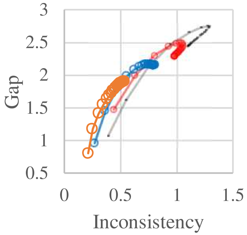
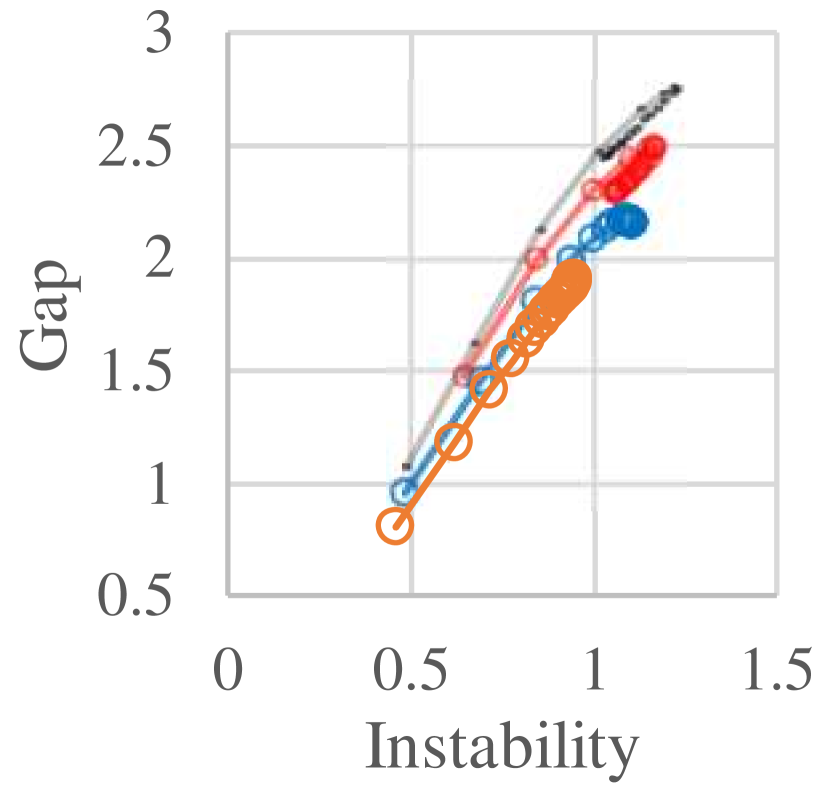
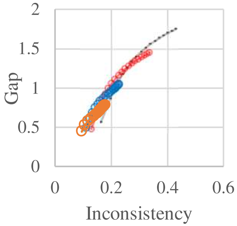
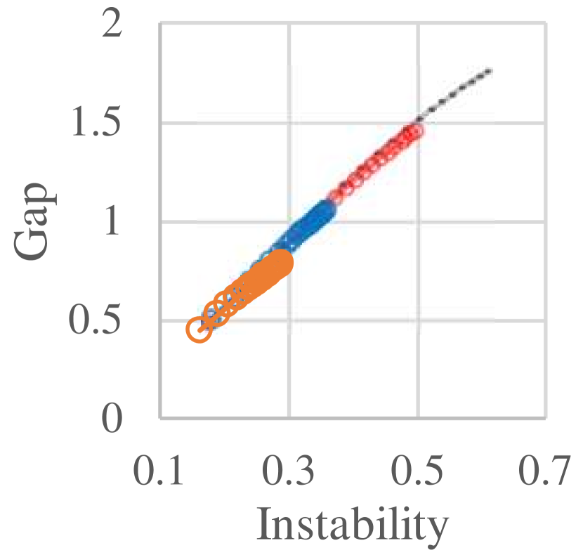
Figure 10 supplements ‘Relation to disagreement’ at the end of Section 2. It shows an example where the behavior of inconsistency is different from disagreement. Training was done on 10% of ImageNet with the seed procedure (tuned to perform well) with training length variations described in Table 9 below. Essentially, in this example, inconsistency goes up like generalization gap, and disagreement goes down like test error and goes up in the end, as training becomes longer.
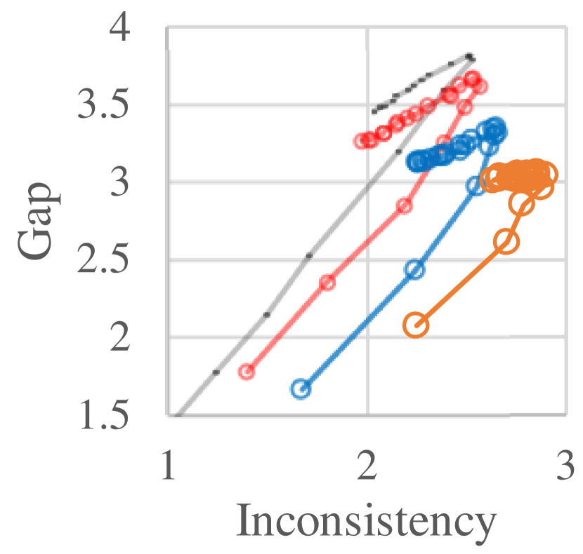
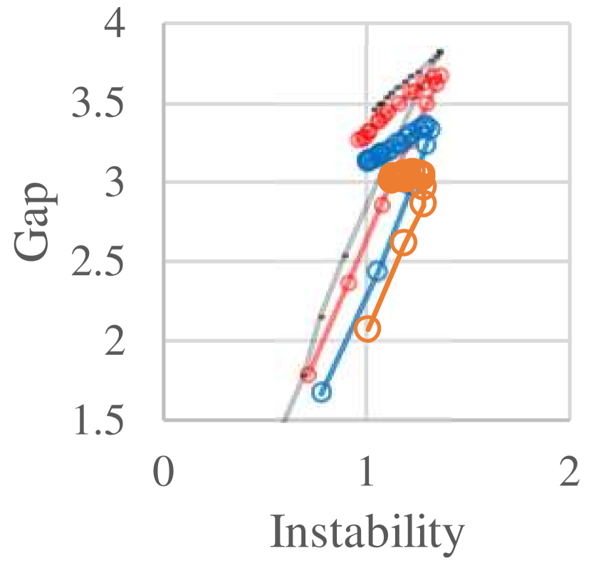
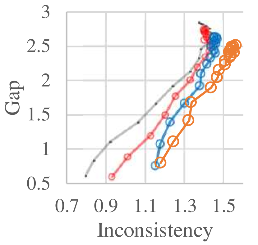
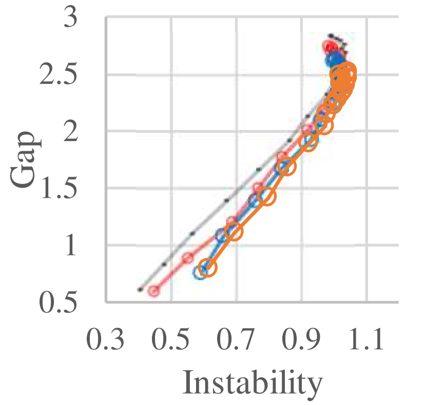
Figure 12 supplements Figure 4 in Section 3.1. It shows inconsistency and instability of model outputs of the models trained with SGD with constant learning rates without iterate averaging. In this setting of high final randomness, larger learning rates make inconsistency larger while instability is mostly unaffected. By contrast, Figure 12 shows that when final randomness is low (due to iterate averaging in this case), both inconsistency and instability are predictive of generalization gap both within and across the learning rates.
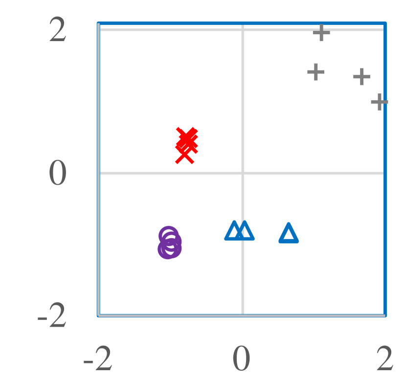
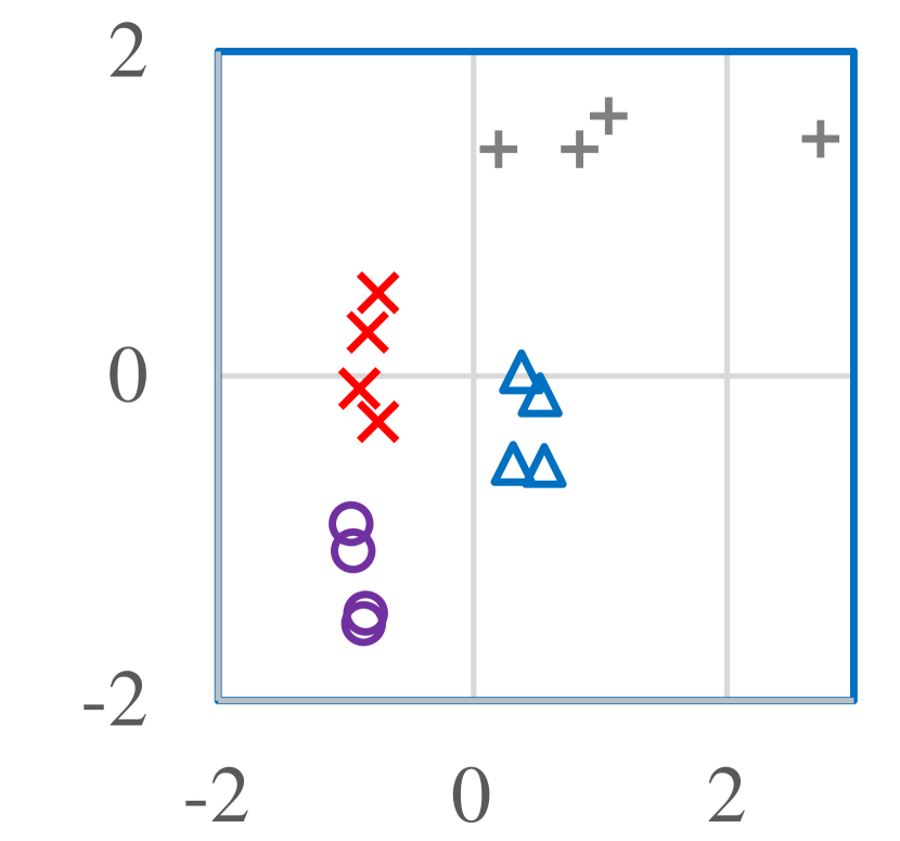
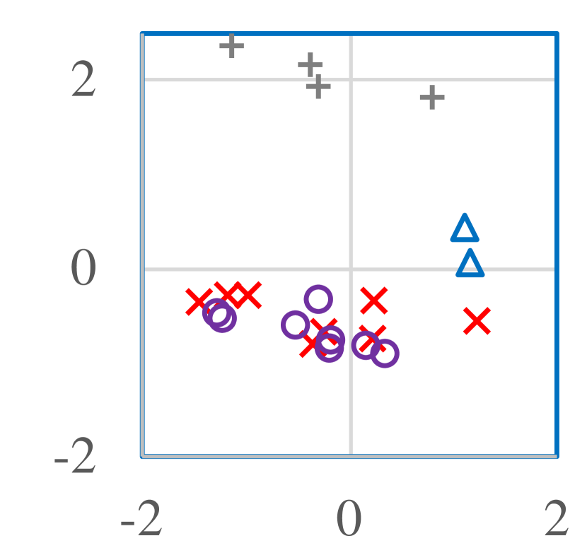
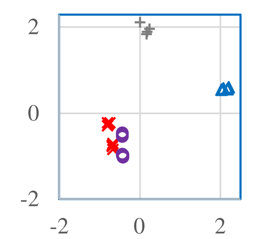
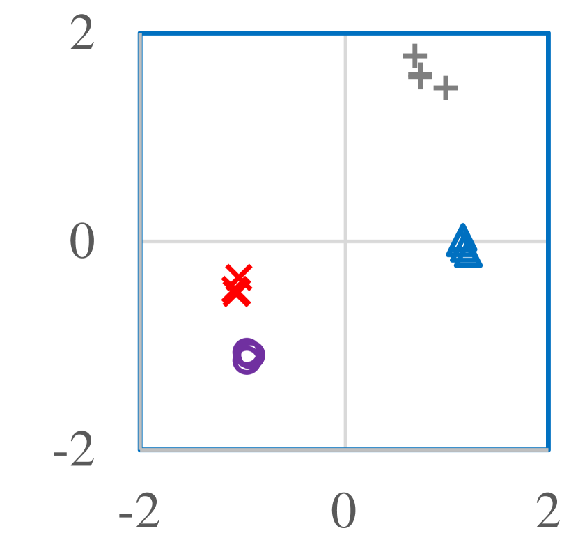
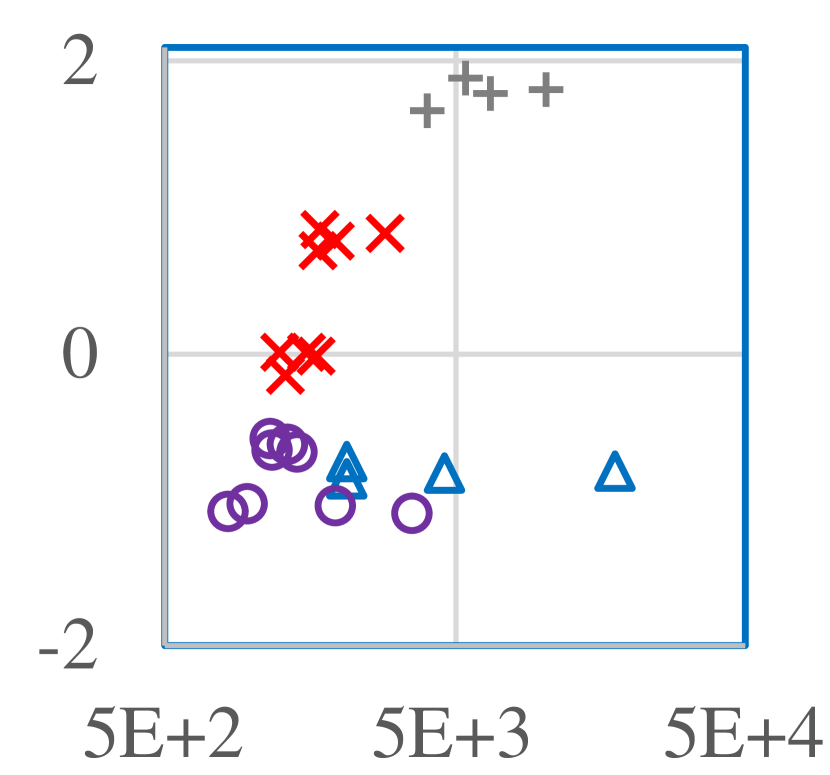
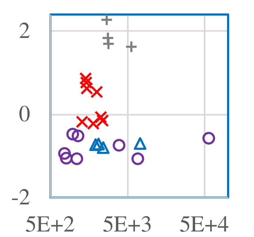
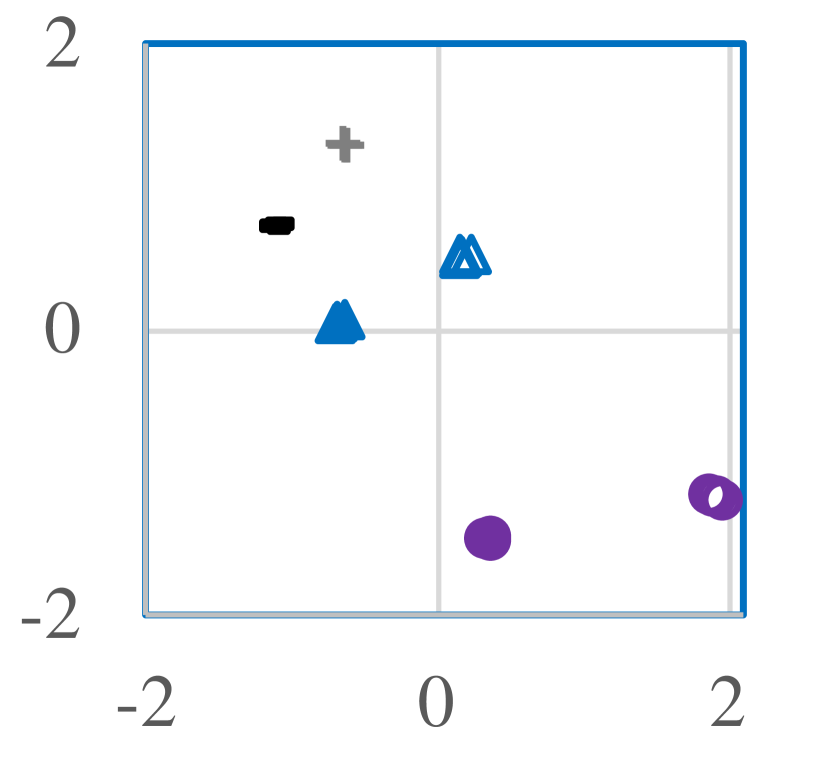
Figure 15–15 supplement Figure 8 in Section 3.2. These figures show the relation of inconsistency and sharpness to generalization gap. Note that each graph has at least 16 points, and some of them (typically for the models trained with the same procedure) are overlapping. Inconsistency shows a stronger correlation with generalization gap than sharpness does.
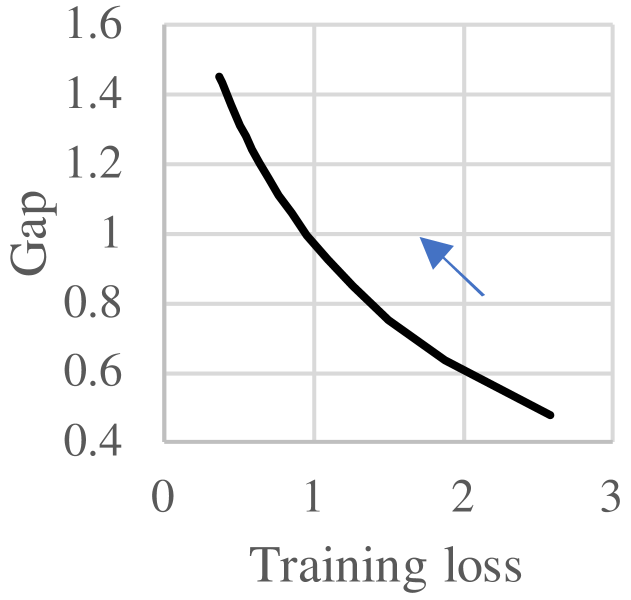
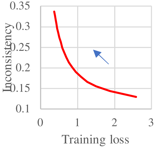
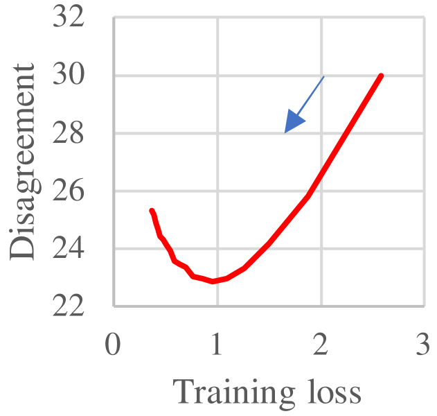

CIFAR-10
CIFAR-100
ImageNet

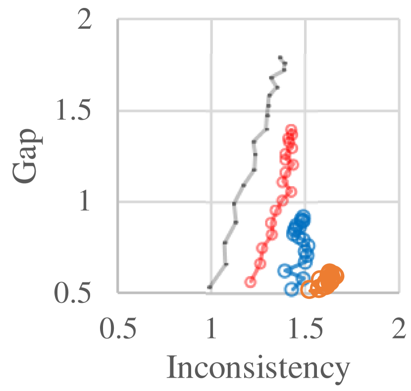
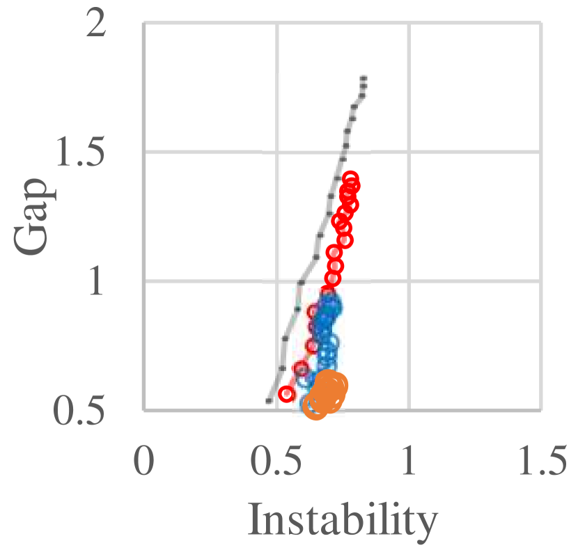
CIFAR-10
CIFAR-100
ImageNet
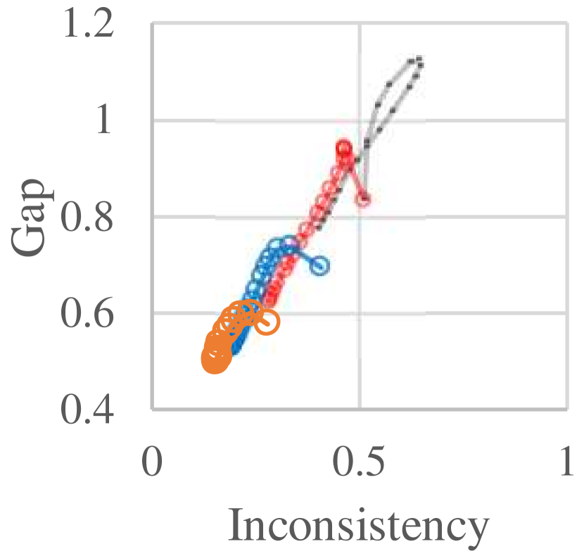
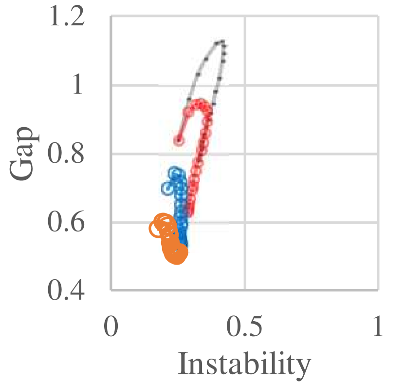
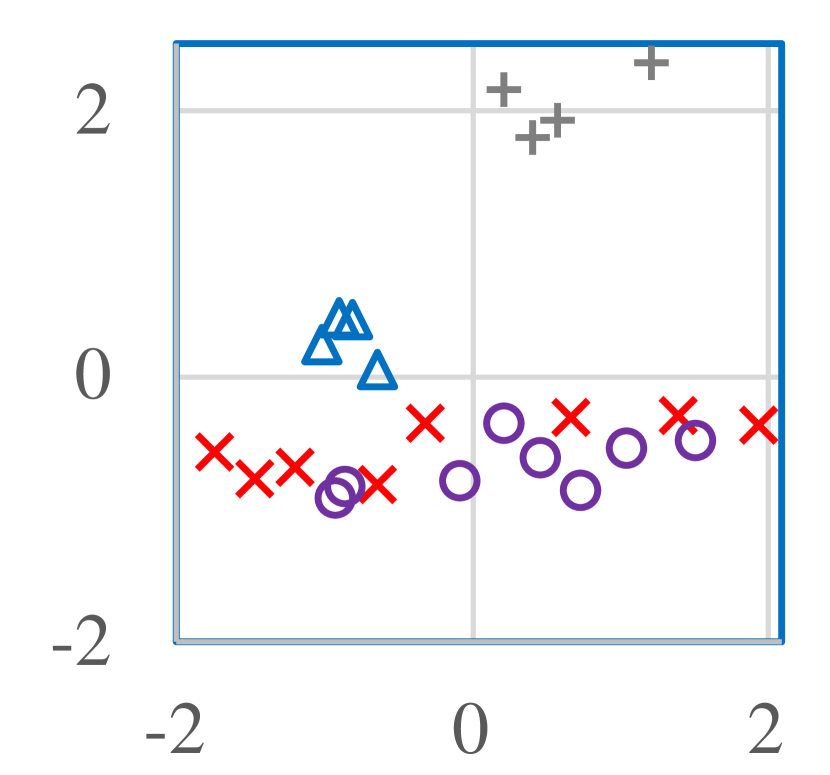
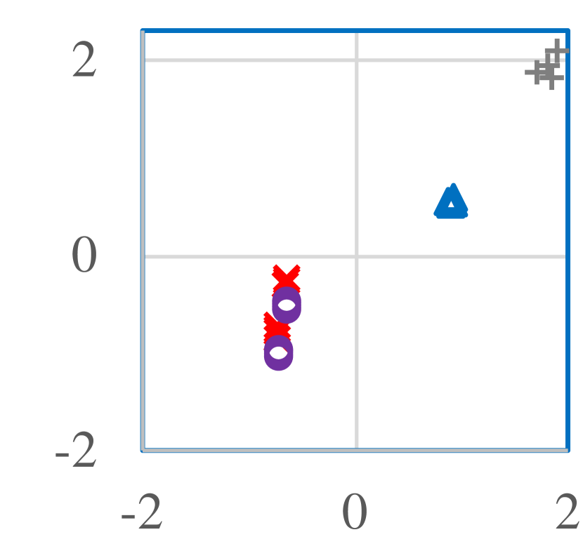
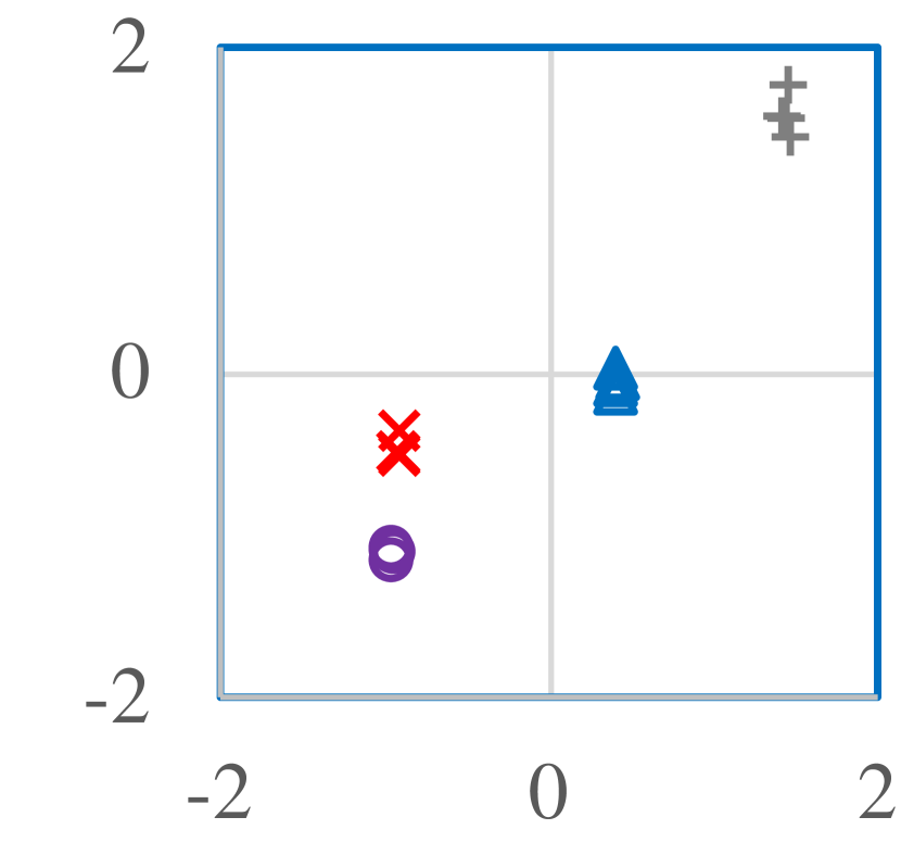
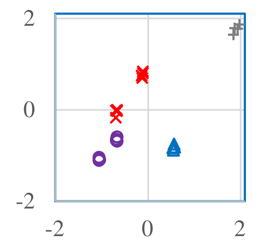
Legend for Case#10 (distillation) △ Teacher standard standard Consist. Consist. Consist+Flat Consist+Flat Student standard Consist. standard Consist. standard Consist.



Appendix C Experimental details
All the experiments were done using GPUs (A100 or older).
C.1 Details of the experiments in Section 3.1
The goal of the experiments reported in Section 3.1 was to find whether/how the predictiveness of is affected by the diversity of the training procedures in comparison. To achieve this goal, we chose the training procedures to experiment with in the following four steps.
-
1.
Choose a network architecture and the size of training set. First, for each dataset, we chose a network architecture and the size of the training set. The training set was required to be smaller than the official set so that disjoint training sets can be obtained for estimating instability. For the network architecture, we chose relatively small residual nets (WRN-28-2 for CIFAR-10/100 and ResNet-50 for ImageNet) to reduce the computational burden.
-
2.
Choose a seed procedure. Next, for each dataset, we chose a procedure that performs reasonably well with the chosen network architecture and the size of training data, and we call this procedure a seed procedure. This was done by referring to the previous studies [32, 10] and performing some tuning on the development data considering that the training data is smaller than in [32, 10]. This step was for making sure to include high-performing (and so practically interesting) procedures in our empirical study.
-
3.
Make core procedures from the seed procedure. For each dataset, we made core procedures from the seed procedure by varying the learning rate, training length, and the presence/absence of iterate averaging. Table 9 shows the resulting core procedures.
- 4.
More precisely, { 25, 50, …, 250, 300, …, 500, 600, …, 1000, 1200, …, 2000 } so that the interval gradually increased from 25 to 200. After training, a few procedures with very high training loss were excluded from the analysis. The cut-off was 0.3 (CIFAR-10), 2.0 (CIFAR-100), and 3.0 (ImageNet), reflecting the number of classes (10, 100, and 1000).
The choice of the constant scheduling is for starting the empirical study with simpler cases by avoiding the complex effects of decaying learning rates, as mentioned in the main paper; also, we found that in these settings, constant learning rates rival the cosine scheduling as long as iterate averaging is performed.
| CIFAR-10/100 | ImageNet | |
| Network | WRN-28-2 | ResNet-50 |
| Training data size | 4K | 120K |
| Learning rate | {0.005, 0.01, 0.025∗, 0.05} | {1/64, 1/32, 1/16∗, 1/8} |
| Weight decay | 2e-3 | 1e-3 |
| Schedule | Constant | Constant |
| Iterate averaging | {EMA∗, None} | {EMA∗, None} |
| Epochs | { 25, …, 1000∗, …, 2000 } | {10, 20, …, 200∗} |
| Mini-batch size | 64 | 512 |
| Data augmentation | Standard+Cutout | Standard |
| Label smoothing | – | 0.1 |
| CIFAR-10 | CIFAR-100 | ImageNet | |
| Network | WRN-16-4 | – | – |
| Weight decay | 5e-4 | – | 1e-4 |
| Schedule | Cosine | Cosine | Cosine |
| Mini-batch size | 256 | 256 | – |
| Data augmentation | None | – | – |
| CIFAR-10 | CIFAR-100 | ImageNet | |
| Network | WRN-28-2 | ResNet-50 | |
| Training data size | 4K | 120K | |
| Weight decay | 2e-3 | 1e-3 | |
| Schedule | Constant | Constant | |
| Mini-batch size | 256 | 64 | 512 |
| Data augmentation | Standard+Cutout | Standard | |
| Label smoothing | – | 0.1 | |
| CIFAR-10 | CIFAR-100 | ImageNet | |
| Weight decay | 5e-4 | 2e-3 | 1e-4 |
| Mini-batch size | 64 | 256 | 512 |
Note that after training, a few procedures with very high training loss were excluded from the analysis (see Table 9 for the cut-off). Right after the model parameter initialization, inconsistency is obviously not predictive of generalization gap since it is non-zero merely reflecting the initial randomness while generalization gap is zero. Similar effects of initial randomness are expected in the initial phase of training; however, these near random models are not of practical interest. Therefore, we excluded from our analysis.
C.1.1 SGD with constant learning rates (Figures 3–4 and 7)
In Section 3.1, we first focused on the effects of varying learning rates and training lengths while fixing anything else, with the training procedures that use a constant learning rate with or without iterate averaging. We analyzed all the subsets of the procedures that met this condition, and reported the common trend. That is, when the learning rate is constant, with iterate averaging, is predictive of generalization gap within and across the learning rates, and without iterate averaging, is predictive of generalization gap only for the procedures that share the learning rate; moreover, without iterate averaging, larger learning rates cause to overestimate generalization gap by larger amounts. Figures 3–4 and 7 show one particular subset for each dataset, and Table 9 shows the values of the attributes fixed in these subsets. To demonstrate the generality of the finding, we show the corresponding figures for one more subset for each dataset in Figures 19–19. The values of the fixed attributes in these subsets are shown in Table 9.

CIFAR-10
CIFAR-100
ImageNet
C.1.2 Procedures with low final randomness (Figures 5 and 7)
The procedures shown in Figures 5 and 7 are subsets (three subsets for three datasets) of all the procedures (the core procedures in Table 9 times the attribute changes in Table 9). The subsets consist of the procedures with either iterate averaging or a vanishing learning rate (i.e., going to zero) so that they meet the condition of low final randomness. These subsets include those with the cosine learning rate schedule. With the cosine schedule, we were interested in not only letting the learning rate go to zero but also stopping the training before the learning rate reaches zero and setting the final model to be the iterate averaging (EMA) at that point, which is well known to be useful (e.g., [32]). Therefore, we trained the models with the cosine schedule for { 250, 500, 1000, 2000 } epochs (CIFAR-10/100) or 200 epochs (ImageNet), and saved the iterate averaging of the models with the interval of one tenth (CIFAR-10/100) or one twentieth (ImageNet) of the entire epochs.
C.2 Details of the experiments in Section 3.2
Section 3.2 studied inconsistency in comparison with sharpness in the settings where these two quantities are reduced by algorithms. The training algorithm with consistency encouragement (co-distillation) is summarized in Algorithm 1. These experiments were designed to study
-
•
practical models trained on full-size training data, and
-
•
diverse models resulting from diverse training settings,
in the situation where algorithms are compared after basic tuning is done, rather than the hyperparameter tuning-like situation in Section 3.1.
C.2.1 Training of the models
| Training type | From scratch | Fine-tuning | Distillation | |||
|---|---|---|---|---|---|---|
| Dataset | ImageNet | Food101 | CIFAR10 | Cars / Dogs | Food101 | |
| Network | ResNet50 | ViT | ViT / Mixer | WRN28-2 | EN-B0 | ResNet-18 |
| Batch size | 512 | 4096 | 512 | 64 | 256 | 512 |
| Epochs | 100 | 300 | 200 / 100 | – | – | 400 |
| Update steps | – | – | – | 500K | 4K / 2K | – |
| Warmup steps | 0 | 10K | 0 | 0 | 0 | 0 |
| Learning rate | 0.125 | 3e-3 | 3e-3 | 0.03 | 0.1 | 0.125 |
| Schedule | Cosine | Linear/Cosine | Cosine | Constant | Cosine | |
| Optimizer | Momentum | AdamW | AdamW | Momentum | Momentum | Momentum |
| Weight decay | 1e-4 | 0.3 | 0.3 | 5e-4 | 1e-5 | 1e-3 |
| Label smooth | 0.1 | 0 | 0.1 | 0 | 0 | 0 |
| Iterate averaging | – | – | – | EMA | EMA | – |
| Gradient clipping | – | 1.0 | 1.0 | – | 20.0 | – |
| Data augment | Standard | Cutout | Standard | |||
| Reference | [10] | [5] | [5] | [10],[32] | [10],[33] | [10] |
| Case# | 1 | 2 | 3 / 4 | 5 | 6 / 7 | 10 |
| ‘Momentum’: SGD with Nesterov momentum 0.9. | ||||||
| Initial learning rate | 1e-5 |
|---|---|
| Learning rate schedule | Linear from to 0.6 |
| Epochs | 4 |
| Batch size | 32 |
| Optimizer | AdamW (=0.9, =0.98, =1e-6) |
| Weight decay | 0.1 |
| Iterate averaging | EMA with momentum 0.999 |
This section describes the experiments for producing the models used in Section 3.2.
Basic settings
Within each of the 10 cases, we used the same basic setting for all, and these shared basic settings were adopted/adapted from the previous studies when possible. Tables 10 and 11 describe the basic settings and the previous studies that were referred to. Some changes to the previous settings were made for efficiency in our computing environment (no TPU); e.g., for Case#1, we changed the batch size from 4096 to 512 and accordingly the learning rate from 1 to 0.125. When adapting the previous settings to new datasets, minimal tuning was done for obtaining reasonable performance, e.g., for Cases#3 and 4, we changed batch size from 4096 to 512 and kept the learning rate without change as it performed better.
For CIFAR-10, following [32], we let the learning rate decay to instead of 0 and set the final model to the EMA of the models with momentum 0.999. For Cases#6–7 (fine-tuning), we used a constant learning rate and used the EMA of the models with momentum 0.999 as the final model, which we found produced reasonable performance with faster training. Cases#6–7 fine-tuned the publicly available EfficientNet-B0111 https://github.com/google-research/sam pretrained with ImageNet by [33]. The dropout rate was set to 0.1 for Case#3, and the stochastic depth drop rate was set to 0.1 for Case#4. The teacher models for Case#10 (distillation) were ensembles of ResNet-18 trained with label smoothing 0.1 for 200 epochs with the same basic setting as the student models (Table 10) otherwise.
For CIFAR-10, the standard data augmentation (shift and horizontal flip) and Cutout [8] were applied. For the other image datasets, only the standard data augmentation (random crop with distortion and random horizontal flip) was applied; the resolution was 224224.
Hyperparameters for SAM
| Case# | 1 | 2 | 3 | 4 | 5 | 6 | 7 | 8,9 | 10 |
| -sharpness | 128 | 256 | 32 | 32 | 32 | 16 | 16 | 2 | 128 |
| 0.05,0.1 | 0.05 | 0.1 | 0.1 | 0.1,0.2 | 0.1,0.2 | 0.1 | 0.005,0.01 | 0.1 |
There are two values that affect the performance of SAM, for -sharpness and the diameter of the neighborhood . Their values are shown in Table 12. [10] found that smaller performs better. However, a smaller can be less efficient as it can reduce the degree of parallelism, depending on the hardware configuration. We made no greater than the reference study in most cases, but for practical feasibility we made it larger for Case#2. was either set according to the reference when possible or chosen on the development data otherwise, from {0.05, 0.1, 0.2} for images and from {0.002, 0.005, 0.01, 0.02, 0.05, 0.1} for texts. For some cases (typically those with less computational burden), we trained the models for one additional value of to have more data points.
Hyperparameters for the inconsistency penalty term
The weight of the inconsistency penalty term for encouraging consistency was fixed to 1.
Number of the models
For each training procedure (identified by the training objective within each case), we obtained 4 models trained with 4 distinct random sequences. Cases#1–9 consisted of either 4 or 6 procedures depending on the number of the values chosen for for SAM. Case#10 (distillation) consisted of 6 procedures222 Although the number of all possible combinations is 16, considering the balance with other cases, we chose to experiment with the following: teacher { ‘Standard’, ‘Consist.’, ‘Consist+Flat’} student { ‘Standard’, ‘Consist.’} , resulting from combining the choice of the training objectives for the teacher and the choice for the student. In total, we had 52 procedures and 208 models.
C.2.2 Estimation of the model-wise inconsistency and sharpness in Section 3.2
When the expectation over the training set was estimated, for a large training set such as ImageNet, 20K data points were sampled for this purpose. As described above, we had 4 models for each of the training procedures. For the procedure without encouragement of low inconsistency, the expectation of the divergence of each model was estimated by taking the average of the divergence from the three other models. As for the procedure with encouragement of low inconsistency, the four models were obtained from two runs as each run produced two models, and so when averaging for estimating inconsistency, we excluded the divergence between the models from the same run due to their dependency.
1-sharpness requires (the diameter of the local region) as input. We set it to the best value for SAM.
C.3 Details of the experiments in Sections 3.3
The optimizer was SGD with Nesterov momentum 0.9.
| Training method | Test error(%) | inconsistency | |
|---|---|---|---|
| Non-ensemble | 17.09±0.20 | 0.30±0.001 | |
| Ensemble of standard models | 14.99±0.05 | 0.14±0.001 | |
| Ensembles of Consist. models | 14.07±0.08 | 0.10±0.001 | |
C.3.1 Ensemble experiments (Figure 9 (a))
The models used in the ensemble experiments were ResNet-18 trained for 200 epochs with label smoothing 0.1 with the basic setting of Case#10 in Table 10 otherwise. Table 13 shows the standard deviation of the values presented in Figure 9 (a). The ensembles also served as the teachers in the distillation experiments.
C.3.2 Distillation experiments (Figure 9 (b))
The student models were ResNet-18 trained for 200 epochs with the basic setting of Case#10 of Table 10 otherwise. The teachers for Figure 9(b) (left) were ResNet-18 ensemble models trained as described in C.3.1. The teachers for Figure 9(b) (middle) were ResNet-50 ensemble models trained similarly. The teachers for Figure 9(b) (right) were EfficientNet-B0 models obtained by fine-tuning the public ImageNet-trained model (footnote 1); fine-tuning was done with encouragement of consistency and flatness (with =0.1) with batch size 512, weight decay 1e-5, the initial learning rate 0.1 with cosign scheduling, gradient clipping 20, and 20K updates. Table 14 shows the standard deviations of the values plotted in Figure 9 (b).
| Test error (%) | inconsistency | |||||
| left | middle | right | left | middle | right | |
| 17.09±0.20 | 0.30±0.001 | |||||
| △ | 15.74±0.09 | 14.95±0.17 | 14.61±0.14 | 0.19±0.001 | 0.21±0.001 | 0.22±0.002 |
| 14.99±0.07 | 14.28±0.11 | 13.89±0.08 | 0.14±0.001 | 0.15±0.001 | 0.14±0.002 | |
| 14.41±0.05 | 13.63±0.09 | 13.06±0.06 | 0.10±0.001 | 0.12±0.001 | 0.08±0.001 | |
C.3.3 Semi-supervised experiments reported in Table 5
The unlabeled data experiments reported in Table 5 used our modification of Algorithm 1, taylored for use of unlabeled data, and it is summarized in Algorithm 2. It differs from Algorithm 1 in two ways. First, to compute the inconsistency penalty term, the model output is compared with that of the exponential moving average (EMA) of the other model, reminiscent of Mean Teacher [34]. The output of the EMA model during the training typically has higher confidence (or lower entropy) than the model itself, and so taking the KL divergence against EMA of the other model serves the purpose of sharpening the pseudo labels and reducing the entropy on unlabeled data. Second, we adopted the masked divergence from Unsupervised Data Augmentation (UDA) [37], which masks (i.e., ignores) the unlabeled instances for which the confidence level of the other model is less than threshold. These changes are effective in the semi-supervised setting (but not in the supervised setting) for preventing the models from getting stuck in a high-entropy region.
In the experiments reported in Table 5, we penalized inconsistency between the model outputs of two training instances of Unsupervised Data Augmentation (UDA) [37], using Algorithm 2, by replacing loss with the UDA objective. The UDA objective penalizes discrepancies between the model outputs for two different data representations (a strongly augmented one and a weakly augmented one) on the unlabeled data (the UDA penalty). The inconsistency penalty term of Algorithm 2 also uses unlabeled data, and for this purpose, we used a strongly augmented unlabeled batch sampled independently of those for the UDA penalty. UDA ‘sharpens’ the model output on the weakly augmented data by scaling the logits, which serves as pseudo labels for unlabeled data, and the degree of sharpening is a tuning parameter. However, we tested UDA without sharpening and obtained better performance on the development data (held-out 5K data points) than reported in [32], and so we decided to use UDA without sharpening for our UDA+‘Consist.’ experiments. We obtained test error 3.95% on the average of 5 independent runs, which is better than 4.33% of UDA alone and 4.25% of FixMatch. Note that each of the 5 runs used a different fold of 4K examples as was done in the previous studies.
Following [32], we used labeled batch size 64, weight decay 5e-4, and updated the weights 500K times with the cosine learning rate schedule decaying from 0.03 to 0.20.03. We set the final model to the average of the last 5% iterates (i.e., the last 25K snapshots of model parameters). We used these same basic settings for all (UDA, FixMatch, and UDA+‘Consist.’). The unlabeled batch size for testing UDA and FixMatch was 647, as in [32]. For computing each of the two penalty terms for UDA+‘Consist.’, we set the unlabeled batch size to 644, which is approximately one half of that for UDA and FixMatch. We made it one half so that the total number of unlabeled data points used by each model (644 for the UDA penalty plus 644 for the inconsistency penalty) becomes similar to that of UDA or FixMatch. RandAugment with the same modification as described in the FixMatch study was used as strong augmentation, and the standard data augmentation (shift and flip) was used as weak augmentation. The threshold for masking was set to 0.5 for both the UDA penalty and the inconsistency penalty and the weights of the both penalties were set to 1. Note that we fixed the weights of penalties to 1, and only tuned the threshold for masking by selecting from on the development data (5K examples).
C.3.4 Fine-tuning experiments in Table 5
The EfficientNet-B4 (EN-B4) fine-tuning experiments reported in Table 5 were done with weight decay 1e-5 (following [10]), batch size 256 and number of updates 20K following the previous studies. We set the learning rate to 0.1 and performed gradient clipping with size 20 to deal with a sudden surge of the gradient size. The diameter of the local region for SAM was chosen from based on the performance of SAM on the development data, and the same chosen value 0.2 was used for both SAM and SAM+‘Consist.’ Following the EN-B7 experiments of [10], the value for -sharpness was set to 16. Since SAM+‘Consist.’ is approximately twice as expensive as SAM as a result of training two models, we also tested SAM with 40K updates (20K2) and found that it did not improve performance. We note that our baseline EN-B4 SAM performance is better than the EN-B7 SAM performance of [10]. This is due to the difference in the basic setting. In [10], EN-B7 was fine-tuned with a larger batch size 1024 with a smaller learning rate 0.016 while the batch normalization statistics was fixed to the pre-trained statistics. Our basic setting allowed a model to go farther away from the initial pre-trained model. Also note that we experimented with smaller EN-B4 instead of EN-B7 due to resource constraints.
| (a) No restriction on training loss | ||||||||||||
|---|---|---|---|---|---|---|---|---|---|---|---|---|
| CIFAR-10 | CIFAR-100 | ImageNet | ||||||||||
| =0 | =0 | =0 | ||||||||||
| Correlation to generalization gap (‘test loss - training loss’) | ||||||||||||
| Inconsist. | 0.23±.01 | 0.38±.01 | 0.60±.05 | 0.69±.01 | 0.51±.01 | 0.55±.01 | 0.68±.06 | 0.81±.01 | 0.75±.01 | 0.75±.01 | 0.73±.17 | 0.92±.00 |
| Disagree. | 0.14±.01 | 0.26±.01 | 0.54±.05 | 0.58±.01 | 0.11±.01 | 0.11±.01 | 0.48±.06 | 0.39±.01 | 0.11±.01 | 0.16±.01 | 0.53±.07 | 0.47±.01 |
| Random | 0.00±.00 | 0.00±.00 | -0.02±.04 | 0.01±.03 | 0.00±.00 | 0.00±.00 | -0.01±.07 | 0.02±.02 | 0.00±.00 | 0.01±.00 | -0.00±.11 | -0.04±.08 |
| Canonical | 0.01±.00 | 0.10±.00 | 0.32±.03 | 0.37±.01 | 0.00±.00 | 0.09±.00 | 0.14±.05 | 0.36±.01 | 0.00±.00 | 0.07±.00 | 0.36±.05 | 0.32±.00 |
| Correlation to test error | ||||||||||||
| Inconsist. | 0.08±.01 | 0.16±.01 | 0.51±.04 | 0.46±.01 | 0.00±.00 | 0.01±.00 | 0.33±.01 | 0.14±.01 | 0.03±.00 | 0.03±.00 | 0.20±.03 | -0.20±.00 |
| Disagree. | 0.31±.01 | 0.37±.00 | 0.58±.05 | 0.68±.00 | 0.19±.01 | 0.31±.02 | 0.57±.05 | 0.63±.01 | 0.04±.00 | 0.05±.00 | 0.30±.07 | 0.25±.01 |
| Random | 0.00±.00 | 0.00±.00 | 0.02±.03 | 0.00±.01 | 0.00±.00 | 0.00±.00 | -0.05±.07 | -0.00±.04 | 0.00±.00 | 0.00±.00 | -0.07±.08 | 0.01±.04 |
| Canonical | 0.01±.00 | 0.03±.00 | 0.15±.02 | 0.20±.01 | 0.00±.00 | 0.19±.01 | 0.31±.15 | 0.49±.01 | 0.00±.00 | 0.03±.00 | 0.08±.03 | 0.18±.00 |
| Correlation to ‘test error - training error’ | ||||||||||||
| Inconsist. | 0.11±.00 | 0.25±.01 | 0.53±.04 | 0.57±.01 | 0.41±.01 | 0.48±.01 | 0.60±.02 | 0.77±.01 | 0.73±.01 | 0.73±.00 | 0.91±.03 | 0.91±.00 |
| Disagree. | 0.16±.01 | 0.28±.01 | 0.54±.07 | 0.60±.01 | 0.12±.01 | 0.12±.01 | 0.45±.05 | 0.40±.01 | 0.12±.01 | 0.16±.01 | 0.52±.06 | 0.46±.01 |
| Random | 0.00±.00 | 0.00±.00 | 0.03±.04 | 0.00±.02 | 0.00±.00 | 0.00±.00 | 0.01±.07 | -0.01±.03 | 0.00±.00 | 0.00±.00 | 0.06±.17 | -0.03±.07 |
| Canonical | 0.01±.00 | 0.07±.00 | 0.31±.06 | 0.31±.01 | 0.00±.00 | 0.09±.00 | 0.21±.09 | 0.35±.01 | 0.00±.00 | 0.07±.00 | 0.24±.02 | 0.32±.00 |
| (b) Excluding the models with very high training loss, as described in Appendix C.1 and Table 9. | ||||||||||||
| CIFAR-10 | CIFAR-100 | ImageNet | ||||||||||
| =0 | =0 | =0 | ||||||||||
| Correlation to generalization gap (‘test loss - training loss’) | ||||||||||||
| Inconsist. | 0.37±.01 | 0.57±.01 | 0.64±.05 | 0.83±.01 | 0.47±.01 | 0.52±.01 | 0.68±.07 | 0.79±.01 | 0.74±.01 | 0.75±.01 | 0.74±.16 | 0.92±.00 |
| Disagree. | 0.34±.02 | 0.53±.02 | 0.61±.05 | 0.80±.02 | 0.26±.03 | 0.33±.01 | 0.60±.05 | 0.65±.01 | 0.24±.02 | 0.33±.02 | 0.61±.07 | 0.65±.01 |
| Random | 0.00±.00 | 0.00±.00 | -0.01±.05 | -0.00±.03 | 0.00±.00 | 0.00±.00 | 0.06±.06 | -0.01±.03 | 0.00±.00 | 0.00±.00 | -0.10±.07 | -0.05±.07 |
| Canonical | 0.02±.00 | 0.15±.00 | 0.28±.04 | 0.44±.01 | 0.00±.00 | 0.21±.01 | 0.23±.06 | 0.52±.01 | 0.00±.00 | 0.10±.00 | 0.46±.16 | 0.38±.00 |
| Correlation to test error | ||||||||||||
| Inconsist. | 0.10±.00 | 0.18±.01 | 0.51±.04 | 0.49±.01 | 0.01±.00 | 0.10±.01 | 0.42±.00 | 0.36±.02 | 0.01±.00 | 0.01±.00 | 0.21±.02 | -0.10±.00 |
| Disagree. | 0.27±.00 | 0.33±.01 | 0.57±.06 | 0.65±.00 | 0.15±.01 | 0.27±.01 | 0.56±.05 | 0.59±.01 | 0.02±.00 | 0.02±.00 | 0.25±.07 | 0.16±.01 |
| Random | 0.00±.00 | 0.00±.00 | 0.03±.03 | 0.01±.02 | 0.00±.00 | 0.00±.00 | 0.04±.07 | 0.02±.02 | 0.00±.00 | 0.00±.00 | 0.04±.10 | 0.01±.06 |
| Canonical | 0.01±.00 | 0.03±.00 | 0.14±.02 | 0.21±.01 | 0.00±.00 | 0.20±.01 | 0.25±.14 | 0.51±.01 | 0.00±.00 | 0.02±.00 | 0.41±.03 | 0.19±.00 |
| Correlation to ‘test error - training error’ | ||||||||||||
| Inconsist. | 0.19±.01 | 0.37±.01 | 0.57±.04 | 0.69±.01 | 0.35±.01 | 0.44±.01 | 0.60±.02 | 0.74±.01 | 0.72±.01 | 0.73±.00 | 0.93±.03 | 0.91±.00 |
| Disagree. | 0.35±.02 | 0.52±.02 | 0.60±.06 | 0.80±.01 | 0.30±.03 | 0.35±.01 | 0.57±.05 | 0.67±.01 | 0.25±.02 | 0.32±.01 | 0.61±.06 | 0.64±.01 |
| Random | 0.00±.00 | 0.00±.00 | 0.01±.06 | -0.02±.01 | 0.00±.00 | 0.00±.00 | -0.01±.08 | 0.01±.03 | 0.00±.00 | 0.00±.00 | -0.02±.09 | -0.06±.06 |
| Canonical | 0.01±.00 | 0.10±.00 | 0.29±.03 | 0.36±.01 | 0.00±.00 | 0.20±.01 | 0.23±.06 | 0.50±.01 | 0.00±.00 | 0.11±.00 | 0.65±.03 | 0.38±.00 |
| (c) Excluding the models with high training loss more aggressively with smaller cut-off values (one half of (b)) | ||||||||||||
| CIFAR-10 | CIFAR-100 | ImageNet | ||||||||||
| =0 | =0 | =0 | ||||||||||
| Correlation to generalization gap (‘test loss - training loss’) | ||||||||||||
| Inconsist. | 0.36±.01 | 0.57±.01 | 0.65±.05 | 0.82±.01 | 0.44±.01 | 0.50±.01 | 0.69±.06 | 0.78±.01 | 0.77±.01 | 0.79±.01 | 0.74±.16 | 0.93±.00 |
| Disagree. | 0.39±.01 | 0.57±.01 | 0.62±.05 | 0.82±.01 | 0.31±.02 | 0.43±.01 | 0.65±.05 | 0.73±.01 | 0.43±.01 | 0.53±.01 | 0.69±.06 | 0.80±.01 |
| Random | 0.00±.00 | 0.00±.00 | 0.02±.03 | 0.00±.02 | 0.00±.00 | 0.00±.00 | 0.03±.11 | 0.04±.02 | 0.00±.00 | 0.00±.00 | -0.05±.12 | -0.02±.03 |
| Canonical | 0.02±.00 | 0.14±.00 | 0.36±.04 | 0.44±.01 | 0.00±.00 | 0.27±.01 | 0.23±.06 | 0.60±.01 | 0.00±.00 | 0.13±.00 | 0.44±.09 | 0.42±.00 |
| Correlation to test error | ||||||||||||
| Inconsist. | 0.12±.01 | 0.21±.01 | 0.53±.04 | 0.53±.01 | 0.04±.00 | 0.19±.01 | 0.48±.00 | 0.50±.02 | 0.01±.00 | 0.01±.00 | 0.31±.02 | 0.13±.00 |
| Disagree. | 0.27±.00 | 0.35±.01 | 0.58±.06 | 0.66±.01 | 0.19±.02 | 0.34±.01 | 0.58±.06 | 0.65±.01 | 0.05±.00 | 0.05±.00 | 0.27±.08 | 0.25±.00 |
| Random | 0.00±.00 | 0.00±.00 | -0.01±.03 | 0.01±.03 | 0.00±.00 | 0.00±.00 | 0.01±.11 | 0.01±.04 | 0.00±.00 | 0.00±.00 | -0.01±.15 | -0.01±.01 |
| Canonical | 0.01±.00 | 0.03±.00 | 0.25±.03 | 0.22±.01 | 0.00±.00 | 0.24±.01 | 0.25±.03 | 0.56±.01 | 0.00±.00 | 0.06±.00 | 0.20±.10 | 0.29±.01 |
| Correlation to ‘test error - training error’ | ||||||||||||
| Inconsist. | 0.18±.01 | 0.37±.01 | 0.58±.04 | 0.68±.01 | 0.30±.01 | 0.42±.01 | 0.61±.02 | 0.72±.01 | 0.72±.01 | 0.76±.00 | 0.93±.03 | 0.92±.00 |
| Disagree. | 0.37±.01 | 0.54±.01 | 0.61±.06 | 0.80±.01 | 0.37±.03 | 0.46±.01 | 0.63±.05 | 0.75±.01 | 0.44±.01 | 0.52±.01 | 0.69±.06 | 0.79±.01 |
| Random | 0.00±.00 | 0.00±.00 | 0.01±.05 | 0.02±.02 | 0.00±.00 | 0.00±.00 | 0.00±.04 | 0.02±.03 | 0.00±.00 | 0.00±.00 | -0.05±.18 | -0.04±.04 |
| Canonical | 0.01±.00 | 0.09±.00 | 0.28±.04 | 0.35±.01 | 0.00±.00 | 0.26±.01 | 0.24±.02 | 0.58±.01 | 0.00±.00 | 0.14±.00 | 0.42±.09 | 0.44±.00 |
Appendix D Additional information
D.1 Additional correlation analyses using the framework of Jiang et al. (2020)
This section reports on the additional correlation analysis using the rigorous framework of Jiang et al. (2020) [18] and shows that the results are consistent with the results in the main paper and the previous work. The analysis uses correlation metrics proposed by [18], which seek to mitigate the effect of what [18] calls spurious correlations that do not reflect causal relationships with generalization. For completeness, we briefly describe below these metrics, and [18] should be referred to for more details and justification.
Notation
In this section, we write for a training procedure (or equivalently, a combination of hyperparameters including the network architecture, the data augmentation method, and so forth). Let be the generalization gap of , and let be the quantity of interest such as inconsistency or disagreement.
Ranking-based
Let be the set of the corresponding pairs of generalization gap and the quantity of interest to be considered: . Then the standard Kendall’s ranking coefficient of can be expressed as:
[18] defines granulated Kendall’s coefficient as:
| (6) |
where is the -th hyperparameter so that , is the set of all possible values for the -th hyperparameter, and .
Mutual information-based
Define , and similarly define . Let be a random variable representing the values of the hyperparameter types in (e.g., = { learning rate, batch size }). Then , the conditional mutual information between and given the set of hyperparameter types, and the conditional entropy can be expressed as follows.
Dividing by for normalization and restricting the size of for enabling computation, [18] defines the metric as:
| (7) |
Results (Tables 15–16)
In Table 15, we show the average and standard deviation of the correlation scores of model-wise quantities (for one model per training procedure), following [18]. The model-wise inconsistency for model trained on with procedure is , and was fixed here; similarly, model-wise disagreement is where is the classification decision of model on data point . The average and standard deviation were computed over 4 independent runs that used 4 distinct subsamples of training sets as training data and distinct random seeds for model parameter initialization, data mini-batching, and so forth.
Table 15 compares inconsistency and disagreement in terms of their correlations with the generalization gap (test loss minus training loss as defined in the main paper), test error, and test error minus training error. The training procedures analyzed here are the procedures that achieve low final randomness by either a vanishing learning rate or iterate averaging as in Figure 5. Tables (a), (b), and (c) differ in the models included in the analysis. As noted in Appendix C.1, since near-random models in the initial phase of training are not of practical interest, procedures with very high training loss were excluded from the analysis in the main paper. Similarly, Table 15-(b) excludes the models with high training loss using the same cut-off values as used in the main paper, and (c) does this with smaller (and therefore more aggressive) cut-off values (one half of (b)), and (a) does not exclude any model. Consequently, the average training loss is the highest in (a) and lowest in (c).
Let us first review Table 15-(a). The results show that inconsistency correlates well to generalization gap (test loss minus training loss) as suggested by our theorem, and disagreement correlates well to test error as suggested by the theorem of the original disagreement study [17]. Regarding ‘test error minus training error’ (last 4 rows): on CIFAR-10, training error is relatively small and so it approaches test error, which explains why disagreement correlates well to it; on the other datasets, ‘test error minus training error’ is more related to ‘test loss minus training loss’, which explains why inconsistency correlates well to it. The standard deviations are relatively small, and so the results are solid. (The standard deviation of tends to be higher than the others for all quantities including the baseline ‘Random’, and this is due to the combination of the macro averaging-like nature of and the smallness of for some ’s, independent of the nature of inconsistency or disagreement.)
The overall trend of Table 15-(b) and (c) is similar to (a). That is, inconsistency correlates well to generalization gap (test loss minus training loss) while disagreement correlates well to test error, consistent with the results in the main paper and the original disagreement study. Comparing (a), (b), and (c), we also note that as we exclude the models with high training loss more aggressively (i.e., going from (a) to (c)), the correlation of disagreement to generalization gap (relative to that of inconsistency) improves and approaches that of inconsistency. For example, on CIFAR-100, the ratio of for (disagreement, generalization gap) with respect to for (inconsistency, generalization gap) improves from (a) 0.11/0.51=22% to (b) 0.26/0.47=55% to (c) 0.31/0.44=70%. With these models, empirically, high training loss roughly corresponds to the low confidence-level on unseen data, and so this observation is consistent with the theoretical insight that when the confidence-level on unseen data is high, disagreement should correlate to generalization gap as well as inconsistency, which is discussed in more detail in Appendix D.3.
| CIFAR-10 | CIFAR-100 | ImageNet | ||||||||||
| MI-based | Ranking | MI-based | Ranking | MI-based | Ranking | |||||||
| =0 | =0 | =0 | ||||||||||
| 0.38 | 0.59 | 0.71 | 0.83 | 0.49 | 0.53 | 0.80 | 0.80 | 0.75 | 0.75 | 0.59 | 0.92 | |
| 0.38 | 0.59 | 0.80 | 0.84 | 0.42 | 0.47 | 0.75 | 0.76 | 0.81 | 0.81 | 0.60 | 0.94 | |
D.2 Training error
Tables 18 and 18 show the training error values (the average, minimum, median, and the maximum) associated with the empirical results reported in Section 3.1 and 3.2, respectively.
| Case#1 | Case#2 | Case#3 | Case#4 | Case#5 | |||||||||||||||
|---|---|---|---|---|---|---|---|---|---|---|---|---|---|---|---|---|---|---|---|
| 10.0 | 8.8 | 10.1 | 11.6 | 4.5 | 2.1 | 4.5 | 6.7 | 0.06 | 0.02 | 0.04 | 0.17 | 0.04 | 0.01 | 0.03 | 0.11 | 0.0 | 0.0 | 0.0 | 0.0 |
| Case#6 | Case#7 | Case#8 | Case#9 | Case#10 | |||||||||||||||
| 0.7 | 0.3 | 0.8 | 1.1 | 0.1 | 0.1 | 0.1 | 0.2 | 4.8 | 3.9 | 4.9 | 5.5 | 2.7 | 1.9 | 2.9 | 3.3 | 2.8 | 0.5 | 1.8 | 6.5 |
D.3 More on inconsistency and disagreement
Inconsistency takes how strongly the models disagree on each data point into account while disagreement ignores it. That is, the information disagreement receives on each data point is binary (whether the classification decisions of two models agree or disagree) while the information inconsistency receives is continuous and more complex. On the one hand, this means that inconsistency could use information ignored by disagreement and thus it could behave quite differently from disagreement as seen in our empirical study. On the other hand, it should be useful also to consider the situation where inconsistency and disagreement are highly correlated since in this case our theoretical results can be regarded as providing a theoretical basis for the correlation of not only inconsistency but also disagreement with generalization gap though indirectly.
To simplify the discussion towards this end, let us introduce a slight variation of Theorem 2.1, which uses 1-norm instead of the KL-divergence since disagreement is related to 1-norm as noted in Section 2.
Proposition D.1 (1-norm variant of Theorem 2.1).
Sketch of proof.
Now suppose that with the models of interest, the confidence level of model outputs is always high so that the highest probability estimate is always near 1, i.e., for any model of interest, we have for a positive constant such that on any unseen data point . Let be the classification decision of on data point as in Section 2: . Then it is easy to show that we have
| (8) |
Disagreement measured for shared training data can be expressed as
| (9) |
Comparing (9) with the definition of above and considering (8), it is clear that under this high-confidence condition, disagreement (9) and 1-norm inconsistency should be highly correlated; therefore, under this condition, Proposition D.1 suggests the relation of disagreement (measured for shared training data) to generalization gap indirectly through .
While this paper focused on the KL-divergence-based inconsistency motivated by the use of the KL-divergence by the existing algorithm for encouraging consistency, the proposition above suggests that 1-norm-based inconsistency might also be useful. We have conducted limited experiments in this regard and observed mixed results. In the settings of Appendix D.1, the correlation scores of 1-norm inconsistency with respect to generalization gap are generally either similar or slightly better, which is promising. As for consistency encouragement during training, we have not seen a clear advantage of using 1-norm inconsistency penalty over using the KL-divergence inconsistency penalty as is done in this paper, and more experiments would be required to understand its advantage/disadvantage.
In our view, however, for the purpose of encouraging consistency during training, KL-divergence inconsistency studied in this paper is more desirable than 1-norm inconsistency in at least three ways. First, minimization of the KL-divergence inconsistency penalty is equivalent to minimization of the standard cross-entropy loss with soft labels provided by the other model; therefore, with the KL-divergence penalty, the training objective can be regarded as a weighted average of two cross-entropy loss terms, which are in the same range (while 1-norm inconsistency is not). This makes tuning of the weight for the penalty more intuitive and easier. Second, optimization of the standard cross-entropy loss term with the KL-divergence inconsistency penalty has an interpretation of functional gradient optimization, as shown in [19]. The last (but not least) point is that optimization may be easier with KL-divergence inconsistency, which is smooth, than with 1-norm inconsistency, which is not smooth.
Related to the last point, disagreement, which involves in the definition, cannot be easily integrated into the training objective, and this is a crucial difference between inconsistency and disagreement from the algorithmic viewpoint.
Finally, we believe that for improving deep neural network training, it is useful to study the connection between generalization and discrepancies of model outputs in general including instability, inconsistency, and disagreement, and we hope that this work contributes to progress in this direction.