Pareto Front Identification with Regret Minimization

Wonyoung Kim
Department of Industrial Engineering
Columbia University
wk2389@columbia.edu
&Garud Iyengar
Department of Industrial Engineering
Columbia University
garud@ieor.columbia.edu
Assaf Zeevi
Graduate School of Business
Columbia University
assaf@gsb.columbia.edu
Abstract

We consider Pareto front identification for linear bandits (PFILin) where the goal is to identify a set of arms whose reward vectors are not dominated by any of the others when the mean reward vector is a linear function of the context. PFILin includes the best arm identification problem and multi-objective active learning as special cases. The sample complexity of our proposed algorithm is $\tilde{O}(d/\Delta^{2})$, where $d$ is the dimension of contexts and $\Delta$ is a measure of problem complexity. Our sample complexity is optimal up to a logarithmic factor. A novel feature of our algorithm is that it uses the contexts of all actions. In addition to efficiently identifying the Pareto front, our algorithm also guarantees $\tilde{O}(\sqrt{d/t})$ bound for instantaneous Pareto regret when the number of samples is larger than $\Omega(d\log dL)$ for $L$ dimensional vector rewards. By using the contexts of all arms, our proposed algorithm simultaneously provides efficient Pareto front identification and regret minimization. Numerical experiments demonstrate that the proposed algorithm successfully identifies the Pareto front while minimizing the regret.

1 Introduction

In Pareto front identification problem, each action or arm has a multidimensional reward vector and the goal is identify the maximal set of arms whose mean reward vectors are not dominated by other arms. This problem arises in a number of fields, e.g. drug trials, healthcare, and e-commerce, where each action has multiple attributes. For example, a drug has associated with its efficacy and a number of different side effects that might be dependent on patient characteristics. In e-commerce, the reward (customer feedback) of an arm (product) includes durability, design, and price.

The typical approach for multi-objective rewards is to create a scalar objective by either taking a weighted combination of all the characteristics (Roijers etΒ al., 2017, 2018; Wanigasekara etΒ al., 2019), or optimizing one characteristic while imposing constraints on the rest (Agrawal and Devanur, 2016; Kim etΒ al., 2023a). This approach requires a new optimization problem if either the weights or the constraints change. It is well known that the optimal actions for any choice of the weights or constraints lie on the Pareto front. Thus, identifying the Pareto front allows us to identify the entire set of actions that are not dominated by others.

The existing literature on Pareto front identificationΒ (PFI) have either focused on the non-contextual multi-armed banditΒ (MAB) settingΒ (Auer etΒ al., 2016) or the setting where the rewards are distributed according to a multivariate Gaussian distribution with the mean given by an unknown function of contextsΒ (Zuluaga etΒ al., 2016). Extension to the linear bandits with general distributions is yet to be studied. Although there is a literature on single-objective best arm identification (BAI) in linear banditsΒ (Soare etΒ al., 2014), the extension to the multi-objective Pareto front identification has not explored. In this paper, we address this gap by introducing the problem of PFI in the linear bandit setting where the mean rewards are linear function of the contextΒ  (PFILin). This problem generalizes both PFI in multi-armed bandits and the best arm identification in linear bandits.

Current algorithms for PFI and BAI in linear bandits do not consider the instantaneous regret incurred during the learning process. This regret is particularly relevant for application such that drug trials and e-commerce where learning occurs by subjecting real patients and customers to potentially sub-optimal actions. In our work, we use techniques from the missing data literature to β€œfill” in the rewards for the unselected arms and utilize all contexts to construct a better Gram matrix for estimating rewards than one that only uses selected contexts. We also adapt randomized regularization techniques by adding artificial noise to some contexts to improve the generalization of the estimator. These methods ensure that we can simultaneously select arms to minimize regret and construct an optimal design for estimating rewards after pure exploration rounds where the number of these rounds is independent of the required accuracy for the Pareto front.

Our main contributions are as follows:

  1. (i)

    We introduce Pareto front identification for linear bandits (PFILin) that generalizes both the BAI problems and PFI for multi-armed bandits.

  2. (ii)

    We develop a novel estimator that leverages techniques from the missing data literature to impute rewards for unselected arms and use all contexts at all decision epochs $t$. Our new estimator ensures $\tilde{O}(\sqrt{d/t})$ ($d=$context dimension) convergence rate for reward vector for all arms, regardless of the particular arm chosen until round $t$. The latter property is extremely important to control regret.

  3. (iii)

    We propose a novel algorithm PFIwR with a PFIΒ sample complexity that is optimal up to logarithmic factors, and additionally, guarantees an $\tilde{O}(\sqrt{d/t})$ Pareto regret after a gap-independent $O(d\log dL)$ exploration rounds for $L$ dimensional rewards.

  4. (iv)

    Our experimental results show that the proposed estimator and algorithm shows superior performance on both synthetic and real dataset.

2 Related Works

The PFILin problem is a generalization of the BAI, which was introduced byΒ Even-Dar etΒ al. (2002) and studied by Soare etΒ al. (2014); Tao etΒ al. (2018) and Jedra and Proutiere (2020), to the vector rewards. Roijers etΒ al. (2017) and Roijers etΒ al. (2018) proposed algorithms for maximizing a weighted sum of reward vectors or a scalar function of reward vectors, respectively. Similarly, Wanigasekara etΒ al. (2019) developed an algorithm for finding an arm that maximizes an unknown scalar function of the reward vectors. However, these methods identify arms that maximize a given scalar function of the reward vectors, rather than identifying the entire set of Pareto optimal arms.

The algorithms for PFI in Gaussian reward settingΒ (Zuluaga etΒ al., 2016; Shah and Ghahramani, 2016) and in non-contextual multi-armed settingΒ (Auer etΒ al., 2016; Ararat and Tekin, 2023) focus on identifying the Pareto front within a certain number of samples, but they do not consider minimizing the Pareto regret in the learning phase. Lu etΒ al. (2019) proposed an algorithm that achieves a bound on Pareto regret for multi-objective contextual bandits, but it does not guarantee the identification of all arms in Pareto front. Degenne etΒ al. (2019) obtained theoretical guarantees for regret minimization and best arm identification under non-contextual single-objective rewards, and Zhong etΒ al. (2021) extended these results to multi-objective rewards. In our work, we establish bounds on both the regret and sample complexity when the reward vector is linear to contexts.

3 Pareto Front Identification for Linear Bandits

In this section, we provide the model and a lower bound of the sample complexity for PFILin. For any positive integer $N\in\mathbb{N}$, let $[N]:={1,\ldots,N}$, and for two real numbers $a,b\in\mathbb{R}$, let $a\wedge b:=\min\{a,b\}$ and $a\vee b:=\max\{a,b\}$. Given a vector $z\in\mathbb{R}^{(L)}$ and $l\in[L]$, we use $z^{(l)}$ to refer to the $l$-th entry of $z$.

At time $t$, the decision-maker observes contexts $\{X_{k,t}:k\in[K]\}$ such that $\|X_{k,t}\|_{2}\leq 1$. After pulling an arm $a_{t}\in[K]$, the decision maker observes a sample of the reward vector $Y_{a_{t},t}\in\mathbb{R}^{L}$, where $Y_{a_{t},t}^{(l)}=X_{a_{t},t}^{\top}\theta_{\star}^{(l)}+\eta_{a_{t},t}^{(l)}$, where $\{\theta_{\star}^{(l)}:l\in[L]\}$ are the unknown (but fixed) parameters. For each $t$, let $\mathcal{H}_{t}$ denote a sigma algebra generated by contexts {Xk,s:k∈[K],s∈[t]}conditional-setsubscriptπ‘‹π‘˜π‘ formulae-sequenceπ‘˜delimited-[]𝐾𝑠delimited-[]𝑑\{X_{k,s}:k\in[K],s\in[t]\}, actions {as:s∈[tβˆ’1]}conditional-setsubscriptπ‘Žπ‘ π‘ delimited-[]𝑑1\{a_{s}:s\in[t-1]\}, and rewards {Yas,s:s∈[tβˆ’1]}conditional-setsubscriptπ‘Œsubscriptπ‘Žπ‘ π‘ π‘ delimited-[]𝑑1\{Y_{a_{s},s}:s\in[t-1]\}. Given $\mathcal{H}_{t}$, for each $k\in[K]$, the error $\eta_{k,t}^{(l)}$ is mean-zero, $1$-sub-Gaussian for each $k\in[K]$. The distribution of contexts may change over time, while they share the same expected values for each arm, i.e., $\mathbb{E}\left[\left.X_{k,t}\right|\mathcal{H}_{t-1},a_{t-1},Y_{a_{t-1},t-1}\right]=x_{k}$ for all $k\in[K]$ and $t\geq 1$. Thus the expected value of the reward is

$$y_{k}^{(l)}:=\mathbb{E}\left[Y_{k,t}^{(l)}\right]=\mathbb{E}\left[\mathbb{E}\left[\left.X_{k,t}\right|\mathcal{H}_{t-1},a_{t-1},Y_{a_{t-1},t-1}\right]^{\top}\theta_{\star}^{(l)}\right]=x_{k}^{\top}\theta_{\star}^{(l)},$$

for all $t\geq 1$ and $l\in[L]$. In this model, we aim to identify the Pareto front from $\{y_{k}\}_{k\in[K]}$ defined as follows.

Definition 1 (Pareto Front).

For two vectors $a$, $b\in\mathbb{R}^{L}$, we define the following orders:

  1. (1)

    Weak domination: $a$ is weakly dominated by $b$, denoted by $a\preceq b$, if $a^{(l)}\leq b^{(l)}$, for all $l\in[L]$.

  2. (2)

    Domination: $a$ is dominated by $b$, denoted by $a\prec b$, if $a$ is weakly dominated by $b$ and there exists $l\in[L]$ such that $a^{(l)}<b^{(l)}$. Further, $a\nprec b$ denotes that $a$ is not dominated by $b$.

  3. (3)

    Strong domination: $a$ is strongly dominated by $b$ denoted as $a\precneqq b$ if $a^{(l)}<b^{(l)}$, for all $l\in[L]$.

An arm is Pareto optimal if it is not dominated by any other arms. The Pareto front $\mathcal{P}_{\star}$ is the set of Pareto optimal arms:

$$\mathcal{P}_{\star}:=\Big{\{}k\in[K]\Big{|}\nexists k^{\prime}:y_{k}\prec y_{k^{\prime}}\Big{\}}.$$ (1)

In order to identify the arms that belong to the Pareto front $\mathcal{P}_{\star}$, the algorithm must estimate the entire set of reward vectors $\{y_{k}\}_{k\in[K]}$. To assess the minimum level of estimation accuracy required for Pareto front identification, we define the distanceΒ Ξ”k⋆subscriptsuperscriptΞ”β‹†π‘˜\Delta^{\star}_{k} of the arm $k$ from the Pareto front. FollowingΒ Auer etΒ al. (2016), we define the degree to which armΒ j𝑗j dominates armΒ kπ‘˜k as follows:

$$m(k,j)=\min\Big{\{}\epsilon\geq 0\Big{|}\exists l\in[L]:y_{k}^{(l)}+\epsilon\geq y_{j}^{(l)}\Big{\}}=0\vee\min_{l\in[L]}\Big{(}y_{j}^{(l)}-y_{k}^{(l)}\Big{)}.$$

We have $m(k,j)>0$ if and only if $y_{k}\precneqq y_{j}$, i.e. armΒ j𝑗j strongly dominates armΒ kπ‘˜k. The distance

$$\Delta_{k}^{\star}:=\max_{k_{\star}\in\mathcal{P}_{\star}}m(k,k_{\star}).$$ (2)

is the minimum amount by which each component of the reward vector $y_{k}$ has to be increased to ensure that armΒ kπ‘˜k is Pareto optimal. The distance $\Delta_{k}^{\star}=0$ for all Pareto optimal arms. With the distance $\Delta_{k}^{\star}$, we present the success condition of PFI.

Definition 2 (PFI success condition).

For any precision $\epsilon>0$ and confidence $\delta\in(0,1)$, a PFIΒ algorithm must output a set of arms $\mathcal{P}\subseteq[K]$ such that

$$\mathcal{P}_{\star}\subseteq\mathcal{P},\;\text{ and }\;\Delta_{k}^{\star}\leq\epsilon,\text{ for all }k\in\mathcal{P}\setminus\mathcal{P}_{\star},$$ (3)

with probability at least $1-\delta$.

The first condition in (3) ensures that $\mathcal{P}$ contains $\mathcal{P}_{\star}$, whereas the second condition ensures that the set $\mathcal{P}$ only contains arms sufficiently close to the Pareto front. Let $\tau_{\epsilon,\delta}$ denote the number of samples required by algorithm to meet the success condition. Then the cumulative regret $R(\tau_{\epsilon,\delta})$ of the algorithm over the interval $[1,\tau_{\epsilon,\delta}]$ is defined as

$$R(\tau_{\epsilon,\delta}):=\sum_{t=1}^{\tau_{\epsilon,\delta}}\Delta_{a_{t}}^{\star}=\sum_{t=1}^{\tau_{\epsilon,\delta}}\max_{k^{\star}\in\mathcal{P}_{\star}}m(a_{t},k^{\star}),$$ (4)

where $a_{t}$ denotes arm selected by the Algorithm. Our goal is to establish an upper bound of the sample complexity $\tau_{\epsilon,\delta}$ while bounding Pareto regret $R(\tau_{\epsilon,\delta})$.

Next, we establish a lower bound for PFILin in terms of a problem complexity measure defined inΒ Auer etΒ al. (2016). First, consider an arm $k$ that is not Pareto optimal. If the arm $k$ is estimated with error greater than $\Delta^{\star}_{k}$, it can erroneously appear Pareto optimal, therefore, we set required accuracy $\Delta_{k}=\Delta^{\star}_{k}$. In BAI, the algorithm terminates successfully when there is only one arm left; thus, the required accuracy is Ξ”=minkβ‰ k⋆⁑ΔkΞ”subscriptπ‘˜superscriptπ‘˜β‹†subscriptΞ”π‘˜\Delta=\min_{k\neq k^{\star}}\Delta_{k}. However, in the PFI problem, several arms can be on the Pareto front, and therefore, one needs another complexity measure to identify all arms on the Pareto front. Let

$$M(k,j):=\min\left\{\epsilon\geq 0\Big{|}\forall l\in[L]:y_{k}^{(l)}\leq y_{j}^{(l)}+\epsilon\right\}=0\vee\max_{l\in[L]}\left(y_{k}^{(l)}-y_{j}^{(l)}\right),$$

denote the amount of the reward values of arm $j$ required to be increased such that $k$ would be weakly dominated by $j$. We have $M(k,j)=0$ if and only if $y_{k}\preceq y_{j}$. Consider a pair of Pareto optimal arms $k$ and $j$. The arm $k$ (resp. $j$) may appear suboptimal if it is underestimated by $M(k,j)$ (resp. $M(j,k)$). Thus, we define the accuracy $\Delta_{k}$ required to prevent misidentifying the Pareto optimal arm $k$ as a suboptimal arm is $\Delta_{k}^{+}:=\min_{k^{\prime}\in\mathcal{P}_{\star}\backslash\{k\}}\min\left\{M(k,k^{\prime}),M(k^{\prime},k)\right\}$. Thus, to identify whether an arm $k\in[K]$ is in Pareto front or not, the estimator must have error less than:

$$\Delta:=\min\Big{\{}\min_{k\notin\mathcal{P}_{\star}}\Delta_{k}^{\star},\min_{k\in\mathcal{P}_{\star}}\Delta_{k}^{+}\Big{\}}$$ (5)

We establish that the required precision $\Delta$ defined inΒ (5) characterizes the lower bound on the number of samples required to solve PFILin.

Theorem 3.1.

[A lower bound of the sample complexity for PFILin.] For $\epsilon>0$, define $\Delta_{\epsilon}:=\max\{\Delta,\epsilon\}$. For any $\delta\in(0,1)$, there exist contexts {Xk,s}k∈[K],s∈[t]subscriptsubscriptπ‘‹π‘˜π‘ formulae-sequenceπ‘˜delimited-[]𝐾𝑠delimited-[]𝑑\{X_{k,s}\}_{k\in[K],s\in[t]}, a set of noise {Ξ·k,s(l)}l∈[L],k∈[K],s∈[t]subscriptsuperscriptsubscriptπœ‚π‘˜π‘ π‘™formulae-sequence𝑙delimited-[]𝐿formulae-sequenceπ‘˜delimited-[]𝐾𝑠delimited-[]𝑑\{\eta_{k,s}^{(l)}\}_{l\in[L],k\in[K],s\in[t]}, and parameters $\{\theta_{\star}^{(l)}\}_{l\in[L]}$ such that any learning algorithm requires at least $\Omega\left(\frac{d}{\Delta_{\epsilon}^{2}}\log\frac{L}{\delta}\right)$ rounds to meet the SuccessΒ ConditionΒ (3).

The proof for lower bound is in AppendixΒ A.2 and is based on the information theoretic analysis on the estimation of $\{\theta_{\star}^{(l)}\}_{l\in[L]}$ (AppendixΒ A.1).

4 Proposed Method

In this section, we present our proposed algorithm with provable guarantees on both PFI sample complexity and regret incurred during learning. The key part of the algorithm is our novel estimator with faster convergence rate than the conventional ridge estimator.

4.1 A Novel Estimator for Pareto Front Identification

The typical learning algorithm in a contextual MAB does not observe rewards unselected arms, and therefore, discards their corresponding contexts. Hence, the algorithm has to typically sample all arms, and this creates a trade-off between minimizing regret and PFI. In contextual linear bandits, recent studies have utilized missing data techniques to impute pseudo-rewards and incorporate contexts of both selected and unselected armsΒ (Kim and Paik, 2019; Kim etΒ al., 2021, 2023b). However, the use of missing data techniques for PFI has not been explored.

For $l\in[L]$, let π’Ÿt(l):={Xk,s:k∈[K],s∈[t]}βˆͺ{Yas,s(l):s∈[t]}assignsuperscriptsubscriptπ’Ÿπ‘‘π‘™conditional-setsubscriptπ‘‹π‘˜π‘ formulae-sequenceπ‘˜delimited-[]𝐾𝑠delimited-[]𝑑conditional-setsuperscriptsubscriptπ‘Œsubscriptπ‘Žπ‘ π‘ π‘™π‘ delimited-[]𝑑\mathcal{D}_{t}^{(l)}:=\{X_{k,s}:k\in[K],s\in[t]\}\cup\{Y_{a_{s},s}^{(l)}:s\in[t]\} denote the data collected up to round $t$ that can inform the estimation of $\theta_{\star}^{(l)}$. At time $t$, we choose $\mathcal{E}_{t}\subset[t]$ with cardinality $\left|\mathcal{E}_{t}\right|$ to be specified later, and add noise to the contexts of unselected arms as follows:

X~k,s:=Xk,s+𝕀​(kβ‰ as)​𝕀​(sβˆˆβ„°t)​Uk,s,Y~k,s(l)=X~k,sβŠ€β€‹ΞΈβ‹†(l)+Ξ·k,s(l),formulae-sequenceassignsubscript~π‘‹π‘˜π‘ subscriptπ‘‹π‘˜π‘ π•€π‘˜subscriptπ‘Žπ‘ π•€π‘ subscriptℰ𝑑subscriptπ‘ˆπ‘˜π‘ superscriptsubscript~π‘Œπ‘˜π‘ π‘™superscriptsubscript~π‘‹π‘˜π‘ topsuperscriptsubscriptπœƒβ‹†π‘™superscriptsubscriptπœ‚π‘˜π‘ π‘™\tilde{X}_{k,s}:=X_{k,s}+\mathbb{I}\left(k\neq a_{s}\right)\mathbb{I}\left(s\in\mathcal{E}_{t}\right)U_{k,s},\quad\tilde{Y}_{k,s}^{(l)}=\tilde{X}_{k,s}^{\top}\theta_{\star}^{(l)}+\eta_{k,s}^{(l)}, (6)

where {Uk,s}k∈[K],sβˆˆβ„°tsubscriptsubscriptπ‘ˆπ‘˜π‘ formulae-sequenceπ‘˜delimited-[]𝐾𝑠subscriptℰ𝑑\{U_{k,s}\}_{k\in[K],s\in\mathcal{E}_{t}} are IID samples from a uniform distribution on $\{x:\left\|x\right\|_{2}\leq 1\}$. Adding noise to data diversifies the direction of contexts Xk,ssubscriptπ‘‹π‘˜π‘ X_{k,s} and improves the estimation. Bishop (1995) showed that adding noise to data is equivalent to Tikhonov regularization which improves generalization performance of the estimator.

However, we do not observe the unselected rewards Y~k,s(l)superscriptsubscript~π‘Œπ‘˜π‘ π‘™\tilde{Y}_{k,s}^{(l)} for kβ‰ atπ‘˜subscriptπ‘Žπ‘‘k\neq a_{t}. Therefore, we combine the missing data and resampling technique to construct and unbiased pseudo-rewards for the missing noisy rewards. In each round $t$, after observing the action $a_{t}$, we generate $t\times\rho_{t}$ independent samples of pseudo-actions {hs​(m):s∈[t],m∈[ρt]}conditional-setsubscriptβ„Žπ‘ π‘šformulae-sequence𝑠delimited-[]π‘‘π‘šdelimited-[]subscriptπœŒπ‘‘\{h_{s}(m):s\in[t],m\in[\rho_{t}]\} from the distribution

Ο•as,s:=p,Ο•k,s=1βˆ’pKβˆ’1​ forΒ β€‹βˆ€kβ‰ asformulae-sequenceassignsubscriptitalic-Ο•subscriptπ‘Žπ‘ π‘ π‘subscriptitalic-Ο•π‘˜π‘ 1𝑝𝐾1Β forΒ for-allπ‘˜subscriptπ‘Žπ‘ \phi_{a_{s},s}:=p,\;\quad\phi_{k,s}=\frac{1-p}{K-1}\;\text{ for }\;\forall k\neq a_{s} (7)

for some $p\in(0,1)$ and $\rho_{t}$ is to be specified later. For $s\in[t]$, Let Ns:=inf{mβ‰₯1:hs​(m)=as}assignsubscript𝑁𝑠infimumconditional-setπ‘š1subscriptβ„Žπ‘ π‘šsubscriptπ‘Žπ‘ N_{s}:=\inf\{m\geq 1:h_{s}(m)=a_{s}\} denote the number of trials until the pseudo-action hs​(m)=assubscriptβ„Žπ‘ π‘šsubscriptπ‘Žπ‘ h_{s}(m)=a_{s}. Using the distribution of the pseudo-action, we compute an inverse probability weighted (IPW) estimate $\widehat{\theta}_{t}^{IPW(l)}$ for $\theta_{\star}^{(l)}$ as follows:

ΞΈ^tI​P​W​(l)=argminθ​[βˆ‘s=1t𝕀​(Ns≀ρt)​(Y~hs​(Ns),s(l)βˆ’X~hs​(Ns),sβŠ€β€‹ΞΈ)2Ο•hs​(Ns),s+Ξ»t​‖θ‖22]superscriptsubscript^πœƒπ‘‘πΌπ‘ƒπ‘Šπ‘™subscriptargminπœƒdelimited-[]superscriptsubscript𝑠1𝑑𝕀subscript𝑁𝑠subscriptπœŒπ‘‘superscriptsuperscriptsubscript~π‘Œsubscriptβ„Žπ‘ subscript𝑁𝑠𝑠𝑙superscriptsubscript~𝑋subscriptβ„Žπ‘ subscript𝑁𝑠𝑠topπœƒ2subscriptitalic-Ο•subscriptβ„Žπ‘ subscript𝑁𝑠𝑠subscriptπœ†π‘‘superscriptsubscriptnormπœƒ22\widehat{\theta}_{t}^{IPW(l)}=\text{argmin}_{\theta}\bigg{[}\sum_{s=1}^{t}\mathbb{I}\left(N_{s}\leq\rho_{t}\right)\frac{\big{(}\tilde{Y}_{h_{s}(N_{s}),s}^{(l)}-\tilde{X}_{h_{s}(N_{s}),s}^{\top}\theta\big{)}^{2}}{\phi_{h_{s}(N_{s}),s}}+\lambda_{t}\left\|\theta\right\|_{2}^{2}\bigg{]} (8)

where $\lambda_{t}$ is the regularization parameter. For each round $s\in[t]$, we add a term to the loss only if $N_{s}\leq\rho_{t}$ where the square loss is observable because hs​(Ns)=assubscriptβ„Žπ‘ subscript𝑁𝑠subscriptπ‘Žπ‘ h_{s}(N_{s})=a_{s}. Using the IPW estimator $\widehat{\theta}_{t}^{IPW(l)}$, we construct the unbiased pseudo-reward

Y^k,s(l)​(m;ΞΈ^tI​P​W​(l)):=(𝕀​(hs​(m)=k)Ο•k,s)​Y~k,s(l)+(1βˆ’π•€β€‹(hs​(m)=k)Ο•k,s)​X~k,sβŠ€β€‹ΞΈ^tI​P​W​(l).assignsuperscriptsubscript^π‘Œπ‘˜π‘ π‘™π‘šsuperscriptsubscript^πœƒπ‘‘πΌπ‘ƒπ‘Šπ‘™π•€subscriptβ„Žπ‘ π‘šπ‘˜subscriptitalic-Ο•π‘˜π‘ superscriptsubscript~π‘Œπ‘˜π‘ π‘™1𝕀subscriptβ„Žπ‘ π‘šπ‘˜subscriptitalic-Ο•π‘˜π‘ superscriptsubscript~π‘‹π‘˜π‘ topsuperscriptsubscript^πœƒπ‘‘πΌπ‘ƒπ‘Šπ‘™\widehat{Y}_{k,s}^{(l)}(m;\widehat{\theta}_{t}^{IPW(l)}):=\left(\frac{\mathbb{I}\left(h_{s}(m)=k\right)}{\phi_{k,s}}\right)\tilde{Y}_{k,s}^{(l)}+\left(1-\frac{\mathbb{I}\left(h_{s}(m)=k\right)}{\phi_{k,s}}\right)\tilde{X}_{k,s}^{\top}\widehat{\theta}_{t}^{IPW(l)}. (9)

Note that Y^k,s(l)​(m;ΞΈ^tI​P​W​(l))superscriptsubscript^π‘Œπ‘˜π‘ π‘™π‘šsuperscriptsubscript^πœƒπ‘‘πΌπ‘ƒπ‘Šπ‘™\widehat{Y}_{k,s}^{(l)}(m;\widehat{\theta}_{t}^{IPW(l)}) is computable when hs​(m)=assubscriptβ„Žπ‘ π‘šsubscriptπ‘Žπ‘ h_{s}(m)=a_{s} because the noise sampled from Uniform distribution is only added to unselected arms, seeΒ (6). Taking conditional the expectation on both sides of Β (9) gives 𝔼​[Y^k,s(l)​(m;ΞΈ^tI​P​W​(l))|β„‹t]=X~k,sβŠ€β€‹ΞΈβ‹†(l)𝔼delimited-[]conditionalsuperscriptsubscript^π‘Œπ‘˜π‘ π‘™π‘šsuperscriptsubscript^πœƒπ‘‘πΌπ‘ƒπ‘Šπ‘™subscriptℋ𝑑superscriptsubscript~π‘‹π‘˜π‘ topsuperscriptsubscriptπœƒβ‹†π‘™\mathbb{E}[\widehat{Y}_{k,s}^{(l)}(m;\widehat{\theta}_{t}^{IPW(l)})|\mathcal{H}_{t}]=\tilde{X}_{k,s}^{\top}\theta_{\star}^{(l)} for all $m\in[\rho_{t}]$. Our proposed estimator is computed as follows:

ΞΈ^t(l)=argminθ​[βˆ‘s=1t𝕀​(Ns≀ρt)​{Y^k,s(l)​(Ns;ΞΈ^tI​P​W​(l))βˆ’X~k,sβŠ€β€‹ΞΈ}2+Ξ»t​‖θ‖22].superscriptsubscript^πœƒπ‘‘π‘™subscriptargminπœƒdelimited-[]superscriptsubscript𝑠1𝑑𝕀subscript𝑁𝑠subscriptπœŒπ‘‘superscriptsuperscriptsubscript^π‘Œπ‘˜π‘ π‘™subscript𝑁𝑠superscriptsubscript^πœƒπ‘‘πΌπ‘ƒπ‘Šπ‘™superscriptsubscript~π‘‹π‘˜π‘ topπœƒ2subscriptπœ†π‘‘superscriptsubscriptnormπœƒ22\widehat{\theta}_{t}^{(l)}=\text{argmin}_{\theta}\bigg{[}\sum_{s=1}^{t}\mathbb{I}\left(N_{s}\leq\rho_{t}\right)\big{\{}\widehat{Y}_{k,s}^{(l)}(N_{s};\widehat{\theta}_{t}^{IPW(l)})-\tilde{X}_{k,s}^{\top}\theta\big{\}}^{2}+\lambda_{t}\left\|\theta\right\|_{2}^{2}\bigg{]}. (10)

The proposed estimatorΒ (10) uses all contexts with unbiased pseudo-rewards when hs​(m)=assubscriptβ„Žπ‘ π‘šsubscriptπ‘Žπ‘ h_{s}(m)=a_{s} for $m\in[\rho_{t}]$, which occurs for all $s\in[t]$ for sufficiently large $\rho_{t}$. We obtain a self-normalized bound for the novel estimator with specified $\lambda_{t}$, $\mathcal{E}_{t}$, and $\rho_{t}$. The challenge in obtaining the bound is to handle the correlation induced between $N_{s}$ and pseudo-rewards Y^k,s(l)​(Ns;ΞΈ^tI​P​W​(l))superscriptsubscript^π‘Œπ‘˜π‘ π‘™subscript𝑁𝑠superscriptsubscript^πœƒπ‘‘πΌπ‘ƒπ‘Šπ‘™\widehat{Y}_{k,s}^{(l)}(N_{s};\widehat{\theta}_{t}^{IPW(l)}) via hs​(m)subscriptβ„Žπ‘ π‘šh_{s}(m), and this is resolved using the decoupling method introduced byΒ DeΒ la Pena and GinΓ© (2012).

Theorem 4.1.

[Self-normalized bound for the novel estimator] For any given $\delta\in(0,1)$, set $\lambda_{t}=4\log\frac{dLt^{2}}{\delta}$, $|\mathcal{E}_{t}|=\big{\lceil}\frac{32(d+2)}{1-p}\log\frac{dLt^{2}}{\delta}\big{\rceil}$, and $\rho_{t}=\lceil\log(\frac{t^{3}}{\delta})/\log(\frac{1}{p})\rceil$. Define the Gram matrix by Vt=βˆ‘s=1t𝕀​(Ns≀ρt)β€‹βˆ‘k=1KX~k,s​X~k,s⊀subscript𝑉𝑑superscriptsubscript𝑠1𝑑𝕀subscript𝑁𝑠subscriptπœŒπ‘‘superscriptsubscriptπ‘˜1𝐾subscript~π‘‹π‘˜π‘ superscriptsubscript~π‘‹π‘˜π‘ topV_{t}=\sum_{s=1}^{t}\mathbb{I}\left(N_{s}\leq\rho_{t}\right)\sum_{k=1}^{K}\tilde{X}_{k,s}\tilde{X}_{k,s}^{\top}. Then, with probability at least $1-4\delta$,

$$\left\|\widehat{\theta}_{t}^{(l)}-\theta_{\star}^{(l)}\right\|_{V_{t}}\leq 8S\sqrt{\log\frac{dLt^{2}}{\delta}}+\frac{4}{p}\sqrt{d\log\frac{L+4Lt/\lambda_{t}}{\delta}},$$ (11)

for all $l\in[L]$ and $t\geq\frac{128(d+2)}{1-p}\big{\{}1+\log\big{(}\frac{64(d+2)}{e(1-p)}\sqrt{\frac{dL}{\delta}}\big{)}\big{\}}$.

Note that the normalizing Gram matrix $V_{t}$ inΒ (11) uses the contexts for all arms instead of only the selected arms in all rounds with high probability for sufficiently large $\rho_{t}$. Previous methods for BAI in linear bandits normalized the error of the estimator by the Gram matrix At=βˆ‘s=1tXas,s​Xas,s⊀+Idsubscript𝐴𝑑superscriptsubscript𝑠1𝑑subscript𝑋subscriptπ‘Žπ‘ π‘ superscriptsubscript𝑋subscriptπ‘Žπ‘ π‘ topsubscript𝐼𝑑A_{t}=\sum_{s=1}^{t}X_{a_{s},s}X_{a_{s},s}^{\top}+I_{d} consisting of the contexts of only the selected arms, and established the following bound:

$$\left|x^{\top}(\widehat{\theta}_{t}-\theta^{\star})\right|\leq\left\|x\right\|_{A_{t}^{-1}}\left\|\widehat{\theta}_{t}-\theta^{\star}\right\|_{A_{t}}\leq\left\|x\right\|_{A_{t}^{-1}}\bigg{(}\sqrt{d\log\frac{1+t}{\delta}}+\left\|\theta^{\star}\right\|_{2}\bigg{)},$$

where $\widehat{\theta}_{t}$ is the least-square estimator for $\theta^{\star}$ using {Xas,s,Yas,s}s∈[t]subscriptsubscript𝑋subscriptπ‘Žπ‘ π‘ subscriptπ‘Œsubscriptπ‘Žπ‘ π‘ π‘ delimited-[]𝑑\{X_{a_{s},s},Y_{a_{s},s}\}_{s\in[t]}. To obtain a tight confidence bound, Soare etΒ al. (2014), Xu etΒ al. (2018) and Jedra and Proutiere (2020) proposed arm selection methods that increases the eigenvalues of the Gram matrix $A_{t}$; however, these methods do not guarantee that the chosen arms have low Pareto regret. In contrast, we use the Gram matrix $V_{t}$ whose eigenvalues are further inflated by using the contexts and pseudo-rewards of all arms and adding artificial noise. In addition, we use a novel decomposition of the error of the estimator:

|1tβ€‹βˆ‘s=1tXk,sβŠ€β€‹ΞΈ^t(l)βˆ’xkβŠ€β€‹ΞΈβ‹†(l)|1𝑑superscriptsubscript𝑠1𝑑superscriptsubscriptπ‘‹π‘˜π‘ topsuperscriptsubscript^πœƒπ‘‘π‘™superscriptsubscriptπ‘₯π‘˜topsuperscriptsubscriptπœƒβ‹†π‘™\displaystyle\left|\frac{1}{t}\sum_{s=1}^{t}X_{k,s}^{\top}\widehat{\theta}_{t}^{(l)}-x_{k}^{\top}\theta_{\star}^{(l)}\right|
≀1t​|βˆ‘s=1tX~k,sβŠ€β€‹(ΞΈ^t(l)βˆ’ΞΈβ‹†(l))|+1t​|βˆ‘s=1t(X~k,sβˆ’xk)βŠ€β€‹ΞΈβ‹†(l)|+1t​|βˆ‘s=1t(X~k,sβˆ’Xk,s)βŠ€β€‹ΞΈ^t(l)|,absent1𝑑superscriptsubscript𝑠1𝑑superscriptsubscript~π‘‹π‘˜π‘ topsuperscriptsubscript^πœƒπ‘‘π‘™superscriptsubscriptπœƒβ‹†π‘™1𝑑superscriptsubscript𝑠1𝑑superscriptsubscript~π‘‹π‘˜π‘ subscriptπ‘₯π‘˜topsuperscriptsubscriptπœƒβ‹†π‘™1𝑑superscriptsubscript𝑠1𝑑superscriptsubscript~π‘‹π‘˜π‘ subscriptπ‘‹π‘˜π‘ topsuperscriptsubscript^πœƒπ‘‘π‘™\displaystyle\leq\frac{1}{t}\left|\sum_{s=1}^{t}\tilde{X}_{k,s}^{\top}\big{(}\widehat{\theta}_{t}^{(l)}-\theta_{\star}^{(l)}\big{)}\right|+\frac{1}{t}\left|\sum_{s=1}^{t}\big{(}\tilde{X}_{k,s}-x_{k}\big{)}^{\top}\theta_{\star}^{(l)}\right|+\frac{1}{t}\left|\sum_{s=1}^{t}\!\big{(}\tilde{X}_{k,s}-X_{k,s}\big{)}^{\top}\widehat{\theta}_{t}^{(l)}\right|,
≀1t​tβ€‹βˆ‘s=1t{X~k,sβŠ€β€‹(ΞΈ^t(l)βˆ’ΞΈβ‹†(l))}2+1t​|βˆ‘s=1t(X~k,sβˆ’xk)βŠ€β€‹ΞΈβ‹†(l)|+1t​|βˆ‘s=1t(X~k,sβˆ’Xk,s)βŠ€β€‹ΞΈ^t(l)|,absent1𝑑𝑑superscriptsubscript𝑠1𝑑superscriptsuperscriptsubscript~π‘‹π‘˜π‘ topsuperscriptsubscript^πœƒπ‘‘π‘™superscriptsubscriptπœƒβ‹†π‘™21𝑑superscriptsubscript𝑠1𝑑superscriptsubscript~π‘‹π‘˜π‘ subscriptπ‘₯π‘˜topsuperscriptsubscriptπœƒβ‹†π‘™1𝑑superscriptsubscript𝑠1𝑑superscriptsubscript~π‘‹π‘˜π‘ subscriptπ‘‹π‘˜π‘ topsuperscriptsubscript^πœƒπ‘‘π‘™\displaystyle\leq\frac{1}{t}\sqrt{t\sum_{s=1}^{t}\Big{\{}\tilde{X}_{k,s}^{\top}\big{(}\widehat{\theta}_{t}^{(l)}-\theta_{\star}^{(l)}\big{)}\Big{\}}^{2}}+\frac{1}{t}\left|\sum_{s=1}^{t}\big{(}\tilde{X}_{k,s}-x_{k}\big{)}^{\top}\theta_{\star}^{(l)}\right|+\frac{1}{t}\left|\sum_{s=1}^{t}\!\big{(}\tilde{X}_{k,s}-X_{k,s}\big{)}^{\top}\widehat{\theta}_{t}^{(l)}\right|,
≀1t​‖θ^t(l)βˆ’ΞΈβ‹†(l)β€–Vt+1t​|βˆ‘s=1t(X~k,sβˆ’xk)βŠ€β€‹ΞΈβ‹†(l)|+1t​|βˆ‘s=1t(X~k,sβˆ’Xk,s)βŠ€β€‹ΞΈ^t(l)|,absent1𝑑subscriptnormsuperscriptsubscript^πœƒπ‘‘π‘™superscriptsubscriptπœƒβ‹†π‘™subscript𝑉𝑑1𝑑superscriptsubscript𝑠1𝑑superscriptsubscript~π‘‹π‘˜π‘ subscriptπ‘₯π‘˜topsuperscriptsubscriptπœƒβ‹†π‘™1𝑑superscriptsubscript𝑠1𝑑superscriptsubscript~π‘‹π‘˜π‘ subscriptπ‘‹π‘˜π‘ topsuperscriptsubscript^πœƒπ‘‘π‘™\displaystyle\leq\frac{1}{\sqrt{t}}\left\|\widehat{\theta}_{t}^{(l)}-\theta_{\star}^{(l)}\right\|_{V_{t}}+\frac{1}{t}\left|\sum_{s=1}^{t}\big{(}\tilde{X}_{k,s}-x_{k}\big{)}^{\top}\theta_{\star}^{(l)}\right|+\frac{1}{t}\left|\sum_{s=1}^{t}\!\big{(}\tilde{X}_{k,s}-X_{k,s}\big{)}^{\top}\widehat{\theta}_{t}^{(l)}\right|,

where second inequality holds by Cauchy-Schwartz inequality. The second and the third term are martingales which is bounded by $\tilde{O}(t^{1/2})$. These results allow us to establish that the reward estimates for all arms converge with the rate of $\tilde{O}(\sqrt{d/t})$ regardless of the arms chosen; and therefore, we are free to choose arms that minimize regret. Define the confidence bound

$$\beta_{t}(\delta):=\frac{1}{\sqrt{t}}\bigg{\{}8S\!\sqrt{\log\!\frac{6dLt^{2}}{\delta}}+\frac{4}{p}\!\sqrt{\!d\log\!\frac{6L+24Lt/\lambda_{t}}{\delta}}+\big{(}5\sqrt{8}S+\frac{4}{p}\!\sqrt{2d}+4\big{)}\!\sqrt{\log\!\frac{6KLt^{2}}{\delta}}\bigg{\}},$$ (12)

and we present the novel convergence result in the following theorem.

Theorem 4.2.

[Uniform error bound for mean reward] For given $\delta\in(0,1)$, set $\lambda_{t}=4\log\frac{6dLt^{2}}{\delta}$, $|\mathcal{E}_{t}|=\lceil\frac{32(d+2)}{1-p}\log\frac{6dLt^{2}}{\delta}\big{\rceil}$, and $\rho_{t}=\lceil\log\frac{6t^{3}}{\delta}/\log\frac{1}{p}\rceil$. Then with probability at least $1-\delta$,

$$\bigg{|}x_{k}^{\top}\theta_{\star}^{(l)}-\frac{1}{t}\sum_{s=1}^{t}X_{k,t}^{\top}\widehat{\theta}_{t}^{(l)}\bigg{|}\leq\beta_{t}(\delta)$$ (13)

for all $l\in[L]$, $k\in[K]$ and $t\geq\frac{128(d+2)}{1-p}\big{\{}1+\log\big{(}\frac{64(d+2)}{e(1-p)}\sqrt{\frac{6dL}{\delta}}\big{)}\big{\}}$.

TheoremΒ 4.2 establishes that the reward estimates for all $k\in[K]$ and $l\in[L]$ converge with the rate of $\tilde{O}(1/\sqrt{t})$ regardless of the arms chosen. This is possible because after $\Omega(d\log\frac{dL}{\delta})$ rounds, the unbiased pseudo-rewards defined inΒ (9) are close to the true rewards. Since we obtain a fast convergence rate for any choice of an arm, we can construct an algorithm that identifies the Pareto front while selecting the arms with low Pareto regret.

Input: accuracy parameter $\epsilon>0$, confidence $\delta>0$, sampling parameter $p\in(0,1)$.
Initialize $\mathcal{A}_{0}=[K]$, $\mathcal{P}_{0}=\emptyset$ and $\widehat{\theta}_{t}^{(1)}=\cdots=\widehat{\theta}_{t}^{(L)}=0$.
whileΒ π’œtβ‰ βˆ…subscriptπ’œπ‘‘\mathcal{A}_{t}\neq\emptysetΒ do
Β Β Β Β Β Β  /* Step 1. Arm selection */
Β Β Β Β Β Β  ifΒ t≀128​(d+2)1βˆ’p​{1+log⁑(64​(d+2)e​(1βˆ’p)​6​d​LΞ΄)}𝑑128𝑑21𝑝164𝑑2𝑒1𝑝6𝑑𝐿𝛿t\leq\frac{128(d+2)}{1-p}\bigg{\{}1+\log\big{(}\frac{64(d+2)}{e(1-p)}\sqrt{\frac{6dL}{\delta}}\big{)}\bigg{\}}Β then
Β Β Β Β Β Β Β Β Β Β Β Β  Sample $a_{t}\in\mathcal{A}_{t-1}$ randomly.
Β Β Β Β Β Β else
Β Β Β Β Β Β Β Β Β Β Β Β Pull $a_{t}\in[K]:\nexists k^{\prime}\in\mathcal{A}_{t-1}\cup\mathcal{P}_{t-1},\widehat{y}_{k,t}\prec\widehat{y}_{k^{\prime},t}\}$ which minimizes Pareto regret.
Β Β Β Β Β Β  end if
Β Β Β Β Β Β /* Step 2. Identifying Pareto arms */
Β Β Β Β Β Β  Update estimator $\{\widehat{\theta}_{t}^{(l)}\}_{l\in[L]}$ as inΒ (10).
Β Β Β Β Β Β  Set $\mathcal{C}_{t}:=\left\{k\in\mathcal{A}_{t-1}\Big{|}\forall k^{\prime}\in\mathcal{A}_{t-1}:\widehat{m}_{t}(k,k^{\prime})\leq 2\beta_{t}\right\}$.
Β Β Β Β Β Β  Set $\mathcal{P}_{t}^{(1)}:=\left\{k\in\mathcal{C}_{t}\Big{|}\forall k^{\prime}\in\mathcal{C}_{t}\backslash\{k\}:\widehat{M}_{t}^{\epsilon}(k,k^{\prime})\geq 2\beta_{t}\right\}$
Β Β Β Β Β Β  Set $\mathcal{P}_{t}^{(2)}:=\left\{k\in\mathcal{P}_{t}^{(1)}\Big{|}\forall k^{\prime}\in\mathcal{C}_{t}\backslash\mathcal{P}_{t}^{(1)}:\widehat{M}_{t}^{\epsilon}(k^{\prime},k)\geq 2\beta_{t}\right\}$.
Β Β Β Β Β Β  Update $\mathcal{P}_{t}\leftarrow\mathcal{P}_{t-1}\cup\mathcal{P}_{t}^{(2)}$, $\mathcal{A}_{t}\leftarrow\mathcal{C}_{t}\backslash\mathcal{P}_{t}^{(2)}$.
end while
Output: $\mathcal{P}_{t}$
AlgorithmΒ 1 Pareto Front Identification with Regret minimization (PFIwR).

4.2 Pareto Front Identification Algorithm for Linear Contextual Bandits

Our proposed algorithm, PFI with regret minimizationΒ (PFIwR), is displayed in AlgorithmΒ 1. Let y^k,t(l)=tβˆ’1β€‹βˆ‘s=1tXk,sβŠ€β€‹ΞΈ^t(l)superscriptsubscript^π‘¦π‘˜π‘‘π‘™superscript𝑑1superscriptsubscript𝑠1𝑑superscriptsubscriptπ‘‹π‘˜π‘ topsuperscriptsubscript^πœƒπ‘‘π‘™\widehat{y}_{k,t}^{(l)}=t^{-1}\sum_{s=1}^{t}X_{k,s}^{\top}\widehat{\theta}_{t}^{(l)} denote the estimate for reward vectors for the arms and define

$\displaystyle\widehat{m}_{t}(k,k^{\prime}):=$ $\displaystyle\min\left\{u\geq 0\Big{|}\exists l\in[L]:\widehat{y}_{k,t}^{(l)}+u\geq\widehat{y}_{k^{\prime},t}^{(l)}\right\},$
$\displaystyle\widehat{M}_{t}^{\epsilon}(k,k^{\prime}):=$ $\displaystyle\min\left\{u\geq 0\big{|}\forall l\in[L]:\widehat{y}_{k,t}^{(l)}+\epsilon\leq\widehat{y}_{k^{\prime},t}^{(l)}+u\right\}.$

PFIwR computes a set $\mathcal{C}_{t}$ by eliminating the suboptimal arms that are dominated by other arms by more than the confidence bound $2\beta_{t}$ defined inΒ (12). Then PFIwR identifies $\epsilon$-near Pareto optimal arms that are not dominated by other arms ($\mathcal{P}^{(1)}_{t}$ and $\mathcal{P}^{(2)}_{t}$). PFIwRΒ randomly samples from the set $\mathcal{A}_{t}$ of undetermined arms for $O(d\log\frac{dL}{\delta})$ rounds to ensure sufficient accuracy in the unbiased pseudo-rewards. After that the algorithm chooses arms that are estimated to be in Pareto front which minimizes regret.

While PFIwRΒ and Auer etΒ al. (2016) share the same arm elimination strategy (Step 2), the arm selection strategy (Step 1) is substantially different. Specifically, Auer etΒ al. (2016) must sample all arms in $\mathcal{A}_{t}$ at each decision point $t$ in order to decide whether they are Pareto optimal; in contrast, after $\Delta$ independent $\Omega(d\log\frac{dL}{\delta})$ rounds, PFIwRΒ only samples arms that have low regret. As proved in TheoremΒ 4.2, sampling arms with low regret does not harm the convergence rate of the estimator and identifying Pareto front. Thus, PFIwRΒ is efficient both in terms of PFI and minimizing regret.

4.3 Sample Complexity and Regret Bounds

In this section, we provide upper bounds on the number of samples required for PFI and Pareto regret.

Theorem 4.3.

[Upper bound on sample complexity] FixΒ Ο΅>0italic-Ο΅0\epsilon>0 and $\delta\in(0,1)$. Define $\Delta_{\epsilon}=\max\{\epsilon,\Delta\}$, where $\Delta$ is the required accuracy defined inΒ (5). Then stopping time $\tau_{\epsilon,\delta}$ of PFIwR is bounded as follows:

$$\tau_{\epsilon,\delta}=\Big{(}\frac{1}{p^{2}}+\frac{1}{1-p}\Big{)}\cdot O\bigg{(}\frac{d}{\Delta_{\epsilon}^{2}}\log\frac{L\max\{d,K\}}{\Delta_{\epsilon}^{2}\delta}\bigg{)}.$$

The explicit finite-sample bound for $\tau_{\epsilon,\delta}$ is in AppendixΒ A.5. The sample complexity is directly proportional to the context dimensionΒ d𝑑d and $\Delta_{\epsilon}^{-2}$, and is optimal to within a logarithm factor of the lower bound in TheoremΒ 3.1. The factor $p^{-2}+(1-p)^{-1}\nearrow\infty$, as $p\searrow 0$ or $p\nearrow 1$, and attains its minimal value for $p\approx 0.639$. When $L=1$, our result recovers the sample complexity bound for the best arm identification in linear bandits (see e.g., Soare etΒ al. (2014); Tao etΒ al. (2018)). Auer etΒ al. (2016) established an upper bound for the sample complexity related to $\Delta_{k}^{-}:=\min_{j\notin\mathcal{P}_{\star}}(M(j,k)+2\Delta^{\star}_{j})$ for $k\in\mathcal{P}_{\star}$. In contrast, our sample complexity bound does not related to $\Delta^{-}_{k}$ because

$$\min_{k\in\mathcal{P}_{\star}}\Delta_{k}^{-}=\min_{k\in\mathcal{P}_{\star}}\min_{j\notin\mathcal{P}_{\star}}\left(M(j,k)+2\Delta_{j}^{\star}\right)\geq 2\min_{j\notin\mathcal{P}_{\star}}\Delta_{j}^{\star}>\min_{j\notin\mathcal{P}_{\star}}\Delta_{j}^{\star}\geq\Delta,$$

and $\Delta_{k}^{-}$ is included in $\Delta$ defined inΒ (5).

Since PFIwR starts choosing regret minimizing arms after $\Omega(d\log\frac{dL}{\delta})$ rounds, we can bound its regret.

Theorem 4.4.

[Bounds for instantaneous and cumulative Pareto regret] For $t\geq\frac{128(d+2)}{1-p}\big{\{}1+\log\big{(}\frac{64(d+2)}{e(1-p)}\sqrt{\frac{6dL}{\delta}}\big{)}\big{\}}$, the action $a_{t}$ selected by PFIwR has a regret $\Delta_{a_{t}}^{\star}\leq 2\beta_{t-1}$, where $\beta_{t}$ is the $\tilde{O}(\sqrt{d/t})$ error bound defined in (12), with probability at least $1-\delta$. The cumulative Pareto regret of PFIwR satisfies

$$R(\tau_{\epsilon,\delta})=\frac{1}{p}\sqrt{\frac{1}{p^{2}}+\frac{1}{1-p}}\cdot O\left(\frac{d}{\Delta_{\epsilon}}\log\frac{L\cdot\max\{K,d\}}{\Delta_{\epsilon}^{2}\delta}\right).$$

The explicit expression for the finite-sample bound is in AppendixΒ A.6. To our knowledge, this is the first instantaneous regret bound for PFI and BAI that ensures the actions with high regret are not chosen very often. The cumulative regret is inversely proportional to the problem complexity measure $\Delta_{\epsilon}$, or equivalently, sublinear in the number of samples required for PFI. In terms of $d$, the regret is linear in $d$ because an additional $\sqrt{d}$ term comes from the confidence bound $\beta_{t}$.

Refer to caption
(a) Estimation error with diverse contexts across arms. The ratio of our proposed estimator to ridge estimator on 2000 samples is 0.73.
Refer to caption
(b) Estimation error with highly correlated contexts across arms. The ratio of our proposed estimator to ridge estimator on 2000 samples is 0.99.
Figure 1: Estimation error of the proposed estimator and conventional ridge estimator. The line and shade represents the average and standard deviation based on 10 independent experiments, respectively. Using contexts of all arms in our proposed estimator is more effective when the direction of the contexts are diverse.
Refer to caption
(a) Identified Pareto front.
Refer to caption
(b) Pareto regret of the proposed algorithm.
Figure 2: Identified Pareto front and Pareto regret of the proposed algorithm with $p=0.1$, $p=0.5$, and $p=0.9$. The line and shade represent the average and standard deviation based on 10 independent experiments, respectively. Too small $p$ makes algorithm use more samples than necessary, and too large $p$ make algorithm stop before the estimator converges to parameters.

5 Experiments

In this section, we report the results of our numerical results exploring the efficacy and performance of our proposed estimator and algorithm.

5.1 Consistency of the Proposed Estimator
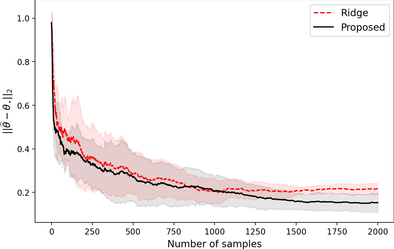
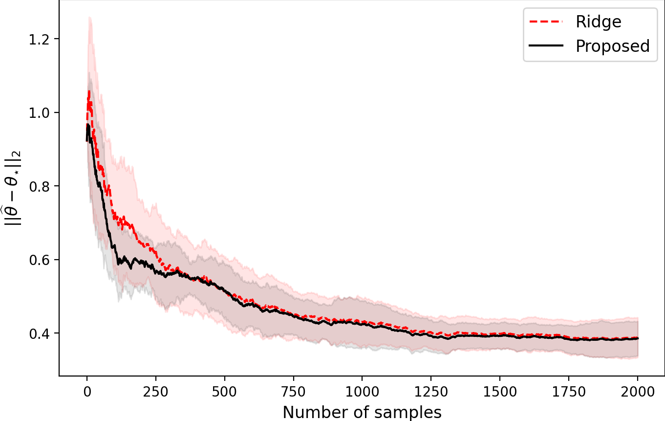
FigureΒ 1 illustrates the $\ell_{2}$ error of the proposed estimator and the ridge estimator as a function of the number of rounds $n$, for $d=10$, $K=10$, and $L=1$. In this experiment, we set the parameter $\theta_{\star}^{(1)}=\mathbf{1}_{d}/\sqrt{d}$, and the mean of contexts’ entries are generated from a Gaussian distribution $\mathcal{N}(\mathbf{0}_{K}^{\top},(1-\rho)I_{K}+\rho\mathbf{1}_{K}\mathbf{1}_{K}^{\top})$. FigureΒ 1(a) and FigureΒ 1(b) present the results of diverse contexts ($\rho=0$) and highly correlated contexts ($\rho=0.9$), respectively.

Our proposed estimator converges faster than the ridge estimator when the mean contexts are generated independently in diverse directions. However, when the mean contexts are highly correlated, the two estimators perform similarly. This is because using contexts and unbiased pseudo-rewards for all arms is more effective when the directions of the mean contexts are diverse.

5.2 Sensitivity of PFIwR to Changes in Hyperparameters
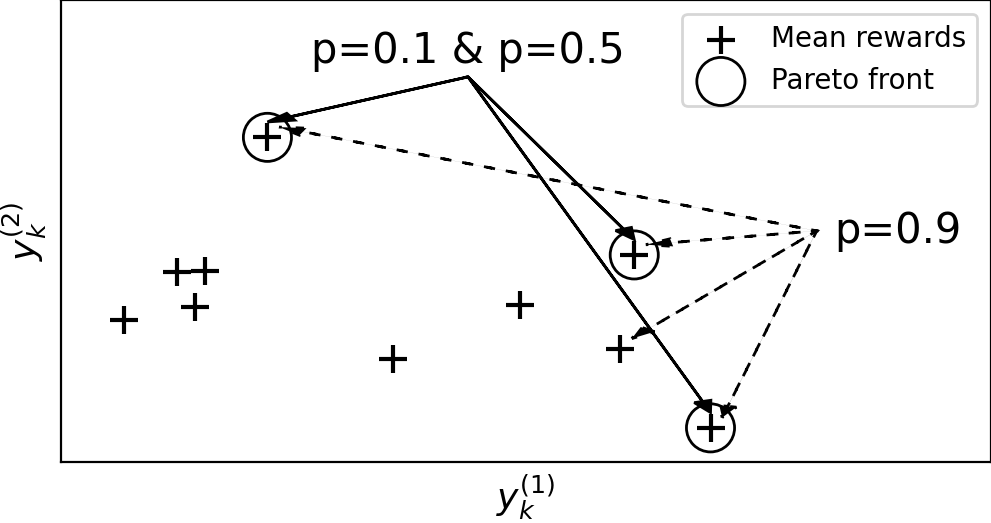
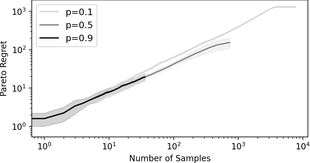
FigureΒ 2 presents the identified Pareto front (FigureΒ 2(a)) and Pareto regret (FigureΒ 2(b)) of the proposed algorithm with $\delta=0.1$ and $\epsilon=0.1$. The mean of contexts is generated in the same way as described in SectionΒ 5.1, with $L=2$ and $\rho=0.5$. Each entry of the $L=2$ parameters are randomly generated from the Uniform distribution supported on the interval $[-1,1]$. All algorithms successfully identified the Pareto fronts, except for the algorithm with $p=0.9$ which misidentifies a near optimal point as Pareto optimal. This shows that setting too large $p$ results in a too small confidence bound $\beta_{t}$, causing the algorithm to make a decision before the estimator converges to the true rewards. For too small $p$, the algorithm is conservative and requires more samples than necessary to identify Pareto fronts. When $p=0.5$, the algorithm terminates right after the Pareto regret is flat which indicates that the algorithm has found the Pareto optimal arms. Based on our results, we recommend setting $p=0.5$ when the estimator converges to be compatible with the decreasing confidence bound.

5.3 Comparison of PFIMulti and PFIwR

Next, we compare PFIwRΒ with PFIMultiΒ Auer etΒ al. (2016) on the SW-LLVM data setΒ (Zuluaga etΒ al., 2016) with the same modification used inΒ Auer etΒ al. (2016) for quasi-stochastic data. (For details, see Section 8 in Auer etΒ al. (2016).)

TableΒ 1 reports the sample complexity results PFIwR and PFIMultiΒ Auer etΒ al. (2016) as a function of $\epsilon\in\{0.0001,0.01,1\}$ with a fixed $\delta$ of $0.1$. The PFIwR algorithm used $p=0.5$. In order to avoid being overly conservative, both algorithms used a tighter confidence bound $\beta$, as suggested byΒ Zuluaga etΒ al. (2016) andΒ Auer etΒ al. (2016). In all cases, PFIwRΒ uses fewer samples than PFIMulti to satisfy the success conditionΒ (3), which is because of our new estimator which converges fast by using contexts and unbiased pseudo-rewards of all contexts.
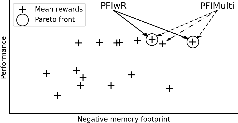
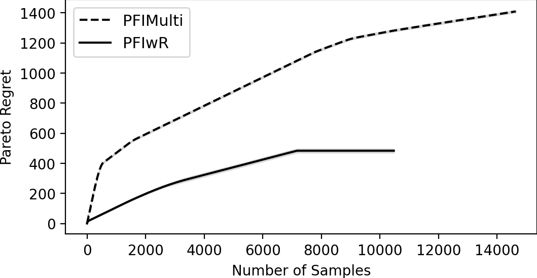
FigureΒ 3(a) and FigureΒ 3(b) display the identified Pareto fronts and Pareto regret PFIwR and PFIMulti for $\delta=0.1$ and $\epsilon=0.01$. In contrast to PFIMulti that misidentifies a suboptimal point as Pareto fronts in most of the independent trials, PFIwR correctly identifies the Pareto front in every trial. PFIwRΒ also has lower regret because it chooses actions that minimize regret after an initial forced exploration rounds. Note that regret minimization does not come at the expense of exploration for PFI since PFIwRΒ is able to use contexts and pseudo-rewards to estimate arm returns.

Table 1: Average and standard deviation of the sample complexity of PFIwR (proposed) and PFIMulti (Auer etΒ al., 2016) based on 100 independent experiments. For all $\epsilon$, our proposed algorithm satisfies the success conditionΒ (3) with fewer number of samples than PFIMulti
Sample complexity $\epsilon=0.0001$ $\epsilon=0.01$ $\epsilon=1$
PFIMulti $15389\pm 299$ $15059\pm 294$ $952\pm 21$
PFIwR $12846\pm 820$ $11921\pm 739$ $68\pm 20$
Refer to caption
(a) Identified Pareto front
Refer to caption
(b) Pareto regret.
Figure 3: Identified Pareto fronts and Pareto regret of PFIwR and LFIMulti on SW-LLVM dataset. The line and shade represent the average and standard deviation based on 100 independent experiments, respectively. Our proposed algorithm (PFIwR) identifies all Pareto optimal arms with less regret compared to that of Auer etΒ al. (2016) (PFIMulti).

References

  • Abbasi-Yadkori etΒ al. [2011] Yasin Abbasi-Yadkori, DΓ‘vid PΓ‘l, and Csaba SzepesvΓ‘ri. Improved algorithms for linear stochastic bandits. In Advances in Neural Information Processing Systems, pages 2312–2320, 2011.
  • Agrawal and Devanur [2016] Shipra Agrawal and Nikhil Devanur. Linear contextual bandits with knapsacks. Advances in Neural Information Processing Systems, 29, 2016.
  • Ararat and Tekin [2023] Cagin Ararat and Cem Tekin. Vector optimization with stochastic bandit feedback. In International Conference on Artificial Intelligence and Statistics, pages 2165–2190. PMLR, 2023.
  • Auer etΒ al. [2016] P.Β Auer, C-K. Chiang, R.Β Ortner, and M.Β Drugan. Pareto front identification from stochastic bandit feedback. In Artificial intelligence and statistics, pages 939–947. PMLR, 2016.
  • Bishop [1995] ChrisΒ M Bishop. Training with noise is equivalent to tikhonov regularization. Neural computation, 7(1):108–116, 1995.
  • Chatzigeorgiou [2013] Ioannis Chatzigeorgiou. Bounds on the lambert function and their application to the outage analysis of user cooperation. IEEE Communications Letters, 17(8):1505–1508, 2013.
  • DeΒ la Pena and GinΓ© [2012] Victor DeΒ la Pena and Evarist GinΓ©. Decoupling: from dependence to independence. Springer Science & Business Media, 2012.
  • Degenne etΒ al. [2019] RΓ©my Degenne, Thomas Nedelec, ClΓ©ment CalauzΓ¨nes, and Vianney Perchet. Bridging the gap between regret minimization and best arm identification, with application to a/b tests. In The 22nd International Conference on Artificial Intelligence and Statistics, pages 1988–1996. PMLR, 2019.
  • Even-Dar etΒ al. [2002] Eyal Even-Dar, Shie Mannor, and Yishay Mansour. Pac bounds for multi-armed bandit and markov decision processes. In COLT, volumeΒ 2, pages 255–270. Springer, 2002.
  • Jedra and Proutiere [2020] Yassir Jedra and Alexandre Proutiere. Optimal best-arm identification in linear bandits. Advances in Neural Information Processing Systems, 33:10007–10017, 2020.
  • Kim and Paik [2019] Gisoo Kim and MyungheeΒ Cho Paik. Doubly-robust lasso bandit. In Advances in Neural Information Processing Systems, pages 5869–5879, 2019.
  • Kim etΒ al. [2021] Wonyoung Kim, Gi-Soo Kim, and MyungheeΒ Cho Paik. Doubly robust thompson sampling with linear payoffs. In Advances in Neural Information Processing Systems, 2021.
  • Kim etΒ al. [2022] Wonyoung Kim, Kyungbok Lee, and MyungheeΒ Cho Paik. Double doubly robust thompson sampling for generalized linear contextual bandits. arXiv preprint arXiv:2209.06983, 2022.
  • Kim etΒ al. [2023a] Wonyoung Kim, Garud Iyengar, and Assaf Zeevi. Improved algorithms for multi-period multi-class packing problems with bandit feedback. arXiv preprint arXiv:2301.13791, 2023a.
  • Kim etΒ al. [2023b] Wonyoung Kim, MyungheeΒ Cho Paik, and Min-Hwan Oh. Squeeze all: Novel estimator and self-normalized bound for linear contextual bandits. In Proceedings of The 26th International Conference on Artificial Intelligence and Statistics, volume 206 of Proceedings of Machine Learning Research, pages 3098–3124. PMLR, 25–27 Apr 2023b.
  • Lu etΒ al. [2019] Shiyin Lu, Guanghui Wang, Yao Hu, and Lijun Zhang. Multi-objective generalized linear bandits. In Proceedings of the 28th International Joint Conference on Artificial Intelligence, pages 3080–3086, 2019.
  • Roijers etΒ al. [2017] DiederikΒ M Roijers, LuisaΒ M Zintgraf, and Ann NowΓ©. Interactive thompson sampling for multi-objective multi-armed bandits. In Algorithmic Decision Theory: 5th International Conference, ADT 2017, Luxembourg, Luxembourg, October 25–27, 2017, Proceedings 5, pages 18–34. Springer, 2017.
  • Roijers etΒ al. [2018] DiederikΒ M Roijers, LuisaΒ M Zintgraf, Pieter Libin, and Ann NowΓ©. Interactive multi-objective reinforcement learning in multi-armed bandits for any utility function. In ALA workshop at FAIM, volumeΒ 8, 2018.
  • Shah and Ghahramani [2016] Amar Shah and Zoubin Ghahramani. Pareto frontier learning with expensive correlated objectives. In International conference on machine learning, pages 1919–1927. PMLR, 2016.
  • Soare etΒ al. [2014] Marta Soare, Alessandro Lazaric, and RΓ©mi Munos. Best-arm identification in linear bandits. Advances in Neural Information Processing Systems, 27, 2014.
  • Tao etΒ al. [2018] Chao Tao, SaΓΊl Blanco, and Yuan Zhou. Best arm identification in linear bandits with linear dimension dependency. In International Conference on Machine Learning, pages 4877–4886. PMLR, 2018.
  • Wanigasekara etΒ al. [2019] Nirandika Wanigasekara, Yuxuan Liang, SiongΒ Thye Goh, YeΒ Liu, JosephΒ Jay Williams, and DavidΒ S Rosenblum. Learning multi-objective rewards and user utility function in contextual bandits for personalized ranking. In IJCAI, pages 3835–3841, 2019.
  • Xu etΒ al. [2018] Liyuan Xu, Junya Honda, and Masashi Sugiyama. A fully adaptive algorithm for pure exploration in linear bandits. In International Conference on Artificial Intelligence and Statistics, pages 843–851. PMLR, 2018.
  • Zhong etΒ al. [2021] Zixin Zhong, WangΒ Chi Cheung, and VincentΒ YF Tan. On the pareto frontier of regret minimization and best arm identification in stochastic bandits. arXiv preprint arXiv:2110.08627, 2021.
  • Zuluaga etΒ al. [2016] Marcela Zuluaga, Andreas Krause, and Markus PΓΌschel. $\varepsilon$-pal: an active learning approach to the multi-objective optimization problem. The Journal of Machine Learning Research, 17(1):3619–3650, 2016.

Appendix A Missing Proofs

A.1 A Lower Bound for Estimation Error

Lemma A.1.

For any $k\in[K]$ and any estimators $\{\widehat{\theta}_{t}^{(l)}\}_{l\in[L]}$, which uses $L\cdot t$ number of observations, there exist $d$-dimensional contexts $\{x_{k}\}_{k\in[K]}$, parameters $\{\theta_{\star}^{(l)}\}_{l\in[L]}$, and noise {Ξ·k,s(l)}l∈[L],k∈[K],sβ‰₯1subscriptsuperscriptsubscriptπœ‚π‘˜π‘ π‘™formulae-sequence𝑙delimited-[]𝐿formulae-sequenceπ‘˜delimited-[]𝐾𝑠1\{\eta_{k,s}^{(l)}\}_{l\in[L],k\in[K],s\geq 1} such that $\|x_{k}\|_{2}\leq 1$ and

$$\min_{l\in[L]}\left|x_{k}^{\top}\left(\widehat{\theta}_{t}^{(l)}-\theta_{l}\right)\right|>\frac{1}{4}\sqrt{\frac{d}{Lt}\log\frac{4L}{\delta}},$$

with probability at least $\delta$.

Proof.

Let $\{e_{i}\}_{i\in[d]}$ denote the Euclidean basis on $\mathbb{R}^{d}$. Let $\phi\in(0,1)$ and $S>0$ be a positve value which will be determined later. For $\phi_{1},\ldots,\phi_{\min\{K,d\}}\in[\phi,1)$, set $x_{i}=\phi_{i}e_{i}$ for $i\in[\min\{K,d\}]$ and $x_{i}=0$ for $i\in(\min\{K,d\},K]$. The random errors {Ξ·k,s(l)}k∈[K],s∈[t],l∈[L]subscriptsuperscriptsubscriptπœ‚π‘˜π‘ π‘™formulae-sequenceπ‘˜delimited-[]𝐾formulae-sequence𝑠delimited-[]𝑑𝑙delimited-[]𝐿\{\eta_{k,s}^{(l)}\}_{k\in[K],s\in[t],l\in[L]} are generated independently from standard Gaussian distribution. For each $l\in[L]$, let $\mathbb{P}_{(\theta_{1},\theta_{2},\ldots,\theta_{L})}^{(t)}$ denote the bandit measure until round $t$, when parameters are set as $(\theta_{\star}^{(1)},\ldots,\theta_{\star}^{(L)})=(\theta_{1},\theta_{2},\ldots,\theta_{L})$. We first prove the result for $l=1$. For each $k\in[K]$ and $S_{k}\in(S/2,S]$,

$$\begin{split}&\sup_{\theta_{1}:\left\|\theta_{1}\right\|_{2}\leq S}\mathbb{P}_{(\theta_{1},\theta_{2},\ldots,\theta_{L})}^{(t)}\left(\left|x_{k}^{\top}\left(\widehat{\theta}_{t}^{(1)}-\theta_{1}\right)\right|>\frac{\phi S}{4}\right)\\ &=\mathbb{P}_{(S_{k}e_{k},\theta_{2},\ldots,\theta_{L})}^{(t)}\left(\left|\phi_{1}e_{k}^{\top}\left(\widehat{\theta}_{t}^{(1)}-S_{k}e_{k}\right)\right|>\frac{\phi S}{4}\right)\\ &\geq\mathbb{P}_{(S_{k}e_{k},\theta_{2},\ldots,\theta_{L})}^{(t)}\left(\left|e_{k}^{\top}\left(\widehat{\theta}_{t}^{(1)}-S_{k}e_{k}\right)\right|>\frac{S}{4}\right)\\ &=\mathbb{P}_{(S_{k}e_{k},\theta_{2},\ldots,\theta_{L})}^{(t)}\left(\left|e_{k}^{\top}\widehat{\theta}_{t}^{(1)}-S_{k}\right|>\frac{S}{4}\right)\\ &\geq\mathbb{P}_{(S_{k}e_{k},\theta_{2},\ldots,\theta_{L})}^{(t)}\left(\left|e_{k}^{\top}\widehat{\theta}_{t}^{(1)}\right|\leq\frac{S}{4}\right),\end{split}$$

where the first inequality holds by $\phi_{1}\geq\phi$ and the last inequality holds by $S_{1}\geq S/2$ and $\{x:\left|x-S_{1}\right|>S/4\}\supseteq\{x:\left|x\right|\leq S/4\}$. For $i\in[d]\backslash\{k\}$,

$\displaystyle\sup_{\theta_{1}:\left\|\theta_{1}\right\|_{2}\leq S}\mathbb{P}_{(\theta_{1},\theta_{2},\ldots,\theta_{L})}^{(t)}\left(\left|x_{k}^{\top}\left(\widehat{\theta}_{t}^{(1)}-\theta_{1}\right)\right|>\frac{\phi S}{4}\right)$
$\displaystyle\geq\sup_{i\in[d]\backslash\{k\}}\mathbb{P}_{(S_{i}e_{i},\theta_{2},\ldots,\theta_{L})}^{(t)}\left(\left|e_{k}^{\top}\left(\widehat{\theta}_{t}^{(1)}-S_{i}e_{i}\right)\right|>\frac{S}{4}\right)$
$\displaystyle\geq\frac{1}{d-1}\sum_{i\in[d]\backslash\{k\}}\mathbb{P}_{(S_{i}e_{i},\theta_{2},\ldots,\theta_{L})}^{(t)}\left(\left|e_{k}^{\top}\left(\widehat{\theta}_{t}^{(1)}-S_{i}e_{i}\right)\right|>\frac{S}{4}\right)$
$\displaystyle\geq\frac{1}{d-1}\sum_{i\in[d]\backslash\{k\}}\mathbb{P}_{(S_{i}e_{i},\theta_{2},\ldots,\theta_{L})}^{(t)}\left(\left|e_{k}^{\top}\widehat{\theta}_{t}^{(1)}\right|>\frac{S}{4}\right)$
$\displaystyle=1-\frac{1}{d-1}\sum_{i\in[d]\backslash\{k\}}\mathbb{P}_{(S_{i}e_{i},\theta_{2},\ldots,\theta_{L})}^{(t)}\left(\left|e_{k}^{\top}\widehat{\theta}_{t}^{(1)}\right|\leq\frac{S}{4}\right).$

Thus,

$\displaystyle\sup_{\theta_{1}:\left\|\theta_{1}\right\|_{2}\leq S}\mathbb{P}_{(\theta_{1},\theta_{2},\ldots,\theta_{L})}^{(t)}\left(\left|x_{k}^{\top}\left(\widehat{\theta}_{t}^{(1)}-\theta_{1}\right)\right|>\frac{\phi S}{4}\right)$
$\displaystyle\geq\frac{1}{2}\mathbb{P}_{(S_{k}e_{k},\theta_{2},\ldots,\theta_{L})}^{(t)}\left(\left|e_{k}^{\top}\widehat{\theta}_{t}^{(1)}\right|\leq\frac{S}{4}\right)$
$\displaystyle\quad+\frac{1}{2}-\frac{1}{2\left(d-1\right)}\sum_{i\in[d]\backslash\{k\}}\mathbb{P}_{(S_{i}e_{i},\theta_{2},\ldots,\theta_{L})}^{(t)}\left(\left|e_{k}^{\top}\widehat{\theta}_{t}^{(1)}\right|\leq\frac{S}{4}\right)$
$\displaystyle=\frac{1}{2}-\frac{1}{2\left(d-1\right)}\sum_{i\in[d]\backslash\{k\}}\left\{\mathbb{P}_{(S_{i}e_{i},\theta_{2},\ldots,\theta_{L})}^{(t)}\left(\left|e_{k}^{\top}\widehat{\theta}_{t}^{(1)}\right|\leq\frac{S}{4}\right)-\mathbb{P}_{(Se_{1},\theta_{2},\ldots,\theta_{L})}^{(t)}\left(\left|e_{k}^{\top}\widehat{\theta}_{t}^{(1)}\right|\leq\frac{S}{4}\right)\right\}$
$\displaystyle\geq\frac{1}{2}-\frac{1}{2\left(d-1\right)}\sum_{i\in[d]\backslash\{k\}}TV\left(\mathbb{P}_{(S_{k}e_{k},\theta_{2},\ldots,\theta_{L})}^{(t)},\mathbb{P}_{(S_{i}e_{i},\theta_{2},\ldots,\theta_{L})}^{(t)}\right),$

where $TV(\mathbb{P}_{1},\mathbb{P}_{2}):=\sup\left|\mathbb{P}_{1}\left(\cdot\right)-\mathbb{P}_{2}\left(\cdot\right)\right|$ is the total variation distance between two probability measures $\mathbb{P}_{1}$ and $\mathbb{P}_{2}$. By Bretagnolle–Huber inequality,

$\displaystyle TV\left(\mathbb{P}_{(S_{k}e_{k},\theta_{2},\ldots,\theta_{L})}^{(t)},\mathbb{P}_{(S_{i}e_{i},\theta_{2},\ldots,\theta_{L})}^{(t)}\right)\leq$ $\displaystyle 1-\frac{1}{2}\exp\left(-D\left(\mathbb{P}_{(S_{k}e_{k},\theta_{2},\ldots,\theta_{L})}^{(t)},\mathbb{P}_{(S_{i}e_{i},\theta_{2},\ldots,\theta_{L})}^{(t)}\right)\right),$

where $D(\mathbb{P}_{1},\mathbb{P}_{2})$ is the relative entropy between two probability measures. Because the errors are standard Gaussian, using the chain rule of the relative entropy,

$\displaystyle D\left(\mathbb{P}_{(S_{k}e_{k},\theta_{2},\ldots,\theta_{L})}^{(t)},\mathbb{P}_{(S_{i}e_{i},\theta_{2},\ldots,\theta_{L})}^{(t)}\right)$
=βˆ‘s=1tD​(β„™(Sk​ek,ΞΈ2,…,ΞΈL)​(Yas,s(l)|β„‹s,as),β„™(Si​ei,ΞΈ2,…,ΞΈL)​(Yas,s(l)|β„‹s,as))absentsuperscriptsubscript𝑠1𝑑𝐷subscriptβ„™subscriptπ‘†π‘˜subscriptπ‘’π‘˜subscriptπœƒ2…subscriptπœƒπΏconditionalsuperscriptsubscriptπ‘Œsubscriptπ‘Žπ‘ π‘ π‘™subscriptℋ𝑠subscriptπ‘Žπ‘ subscriptβ„™subscript𝑆𝑖subscript𝑒𝑖subscriptπœƒ2…subscriptπœƒπΏconditionalsuperscriptsubscriptπ‘Œsubscriptπ‘Žπ‘ π‘ π‘™subscriptℋ𝑠subscriptπ‘Žπ‘ \displaystyle=\sum_{s=1}^{t}D\left(\mathbb{P}_{(S_{k}e_{k},\theta_{2},\ldots,\theta_{L})}(Y_{a_{s},s}^{(l)}|\mathcal{H}_{s},a_{s}),\mathbb{P}_{(S_{i}e_{i},\theta_{2},\ldots,\theta_{L})}(Y_{a_{s},s}^{(l)}|\mathcal{H}_{s},a_{s})\right)
=βˆ‘s=1t𝔼θ1=Sk​ek​[{xasβŠ€β€‹(Si​eiβˆ’Sk​ek)}22]absentsuperscriptsubscript𝑠1𝑑subscript𝔼subscriptπœƒ1subscriptπ‘†π‘˜subscriptπ‘’π‘˜delimited-[]superscriptsuperscriptsubscriptπ‘₯subscriptπ‘Žπ‘ topsubscript𝑆𝑖subscript𝑒𝑖subscriptπ‘†π‘˜subscriptπ‘’π‘˜22\displaystyle=\sum_{s=1}^{t}\mathbb{E}_{\theta_{1}=S_{k}e_{k}}\left[\frac{\left\{x_{a_{s}}^{\top}\left(S_{i}e_{i}-S_{k}e_{k}\right)\right\}^{2}}{2}\right]
≀S2​ϕ22β€‹βˆ‘s=1t𝔼θ1=Sk​ek​[𝕀​(as=1)+𝕀​(as=i)].absentsuperscript𝑆2superscriptitalic-Ο•22superscriptsubscript𝑠1𝑑subscript𝔼subscriptπœƒ1subscriptπ‘†π‘˜subscriptπ‘’π‘˜delimited-[]𝕀subscriptπ‘Žπ‘ 1𝕀subscriptπ‘Žπ‘ π‘–\displaystyle\leq\frac{S^{2}\phi^{2}}{2}\sum_{s=1}^{t}\mathbb{E}_{\theta_{1}=S_{k}e_{k}}\left[\mathbb{I}\left(a_{s}=1\right)+\mathbb{I}\left(a_{s}=i\right)\right].

Thus,

$\displaystyle\sup_{\theta_{1}:\left\|\theta_{1}\right\|_{2}\leq S}\mathbb{P}_{(\theta_{1},\theta_{2},\ldots,\theta_{L})}^{(t)}\left(\left|x_{k}^{\top}\left(\widehat{\theta}_{t}^{(1)}-\theta_{1}\right)\right|>\frac{\phi S}{4}\right)$
$\displaystyle\geq\frac{1}{2}-\frac{1}{2\left(d-1\right)}\sum_{i\in[d]\backslash\{k\}}TV\left(\mathbb{P}_{(Se_{1},\theta_{2},\ldots,\theta_{L})}^{(t)},\mathbb{P}_{(Se_{i},\theta_{2},\ldots,\theta_{L})}^{(t)}\right)$
β‰₯14​(dβˆ’1)β€‹βˆ‘i=2dexp⁑(βˆ’S2​ϕ22β€‹βˆ‘s=1t𝔼θ1=Sk​ek​[𝕀​(as=1)+𝕀​(as=i)])absent14𝑑1superscriptsubscript𝑖2𝑑superscript𝑆2superscriptitalic-Ο•22superscriptsubscript𝑠1𝑑subscript𝔼subscriptπœƒ1subscriptπ‘†π‘˜subscriptπ‘’π‘˜delimited-[]𝕀subscriptπ‘Žπ‘ 1𝕀subscriptπ‘Žπ‘ π‘–\displaystyle\geq\frac{1}{4\left(d-1\right)}\sum_{i=2}^{d}\exp\left(-\frac{S^{2}\phi^{2}}{2}\sum_{s=1}^{t}\mathbb{E}_{\theta_{1}=S_{k}e_{k}}\left[\mathbb{I}\left(a_{s}=1\right)+\mathbb{I}\left(a_{s}=i\right)\right]\right)
β‰₯14​exp⁑(βˆ’S2​ϕ22​(dβˆ’1)β€‹βˆ‘i=2dβˆ‘s=1t𝔼θ1=Sk​ek​[𝕀​(as=1)+𝕀​(as=i)])absent14superscript𝑆2superscriptitalic-Ο•22𝑑1superscriptsubscript𝑖2𝑑superscriptsubscript𝑠1𝑑subscript𝔼subscriptπœƒ1subscriptπ‘†π‘˜subscriptπ‘’π‘˜delimited-[]𝕀subscriptπ‘Žπ‘ 1𝕀subscriptπ‘Žπ‘ π‘–\displaystyle\geq\frac{1}{4}\exp\left(-\frac{S^{2}\phi^{2}}{2\left(d-1\right)}\sum_{i=2}^{d}\sum_{s=1}^{t}\mathbb{E}_{\theta_{1}=S_{k}e_{k}}\left[\mathbb{I}\left(a_{s}=1\right)+\mathbb{I}\left(a_{s}=i\right)\right]\right)
$\displaystyle\geq\frac{1}{4}\exp\left(-\frac{S^{2}\phi^{2}t}{2\left(d-1\right)}\right).$

where the third inequality holds by Jensen’s inequality and the last inequality holds because as∈[K]subscriptπ‘Žπ‘ delimited-[]𝐾a_{s}\in[K]. Setting $\phi=\frac{\sqrt{d}}{S\sqrt{Lt}}\sqrt{\log\frac{4L}{\delta}}\leq\frac{\sqrt{2(d-1)}}{S\sqrt{t}}\sqrt{\log\frac{4}{\delta^{1/L}}}$ gives

$$\sup_{\theta_{1}:\left\|\theta_{1}\right\|_{2}\leq S}\mathbb{P}_{(\theta_{1},\theta_{2},\ldots,\theta_{L})}^{(t)}\left(\left|x_{1}^{\top}\left(\widehat{\theta}_{t}^{(1)}-\theta_{1}\right)\right|>\frac{1}{4}\sqrt{\frac{d}{Lt}\log\frac{4L}{\delta}}\right)\geq\delta^{1/L}.$$

Because the distributions of {Ξ·k,s(l)}l∈[L]subscriptsuperscriptsubscriptπœ‚π‘˜π‘ π‘™π‘™delimited-[]𝐿\{\eta_{k,s}^{(l)}\}_{l\in[L]} are independent,

$\displaystyle\sup_{\theta_{1},\ldots,\theta_{L}\in\Theta}\mathbb{P}_{(\theta_{1},\theta_{2},\ldots,\theta_{L})}^{(t)}\left(\min_{l\in[L]}\left|x_{1}^{\top}\left(\widehat{\theta}_{t}^{(l)}-\theta_{l}\right)\right|>\frac{1}{4}\sqrt{\frac{d}{Lt}\log\frac{4L}{\delta}}\right)$
$\displaystyle=\sup_{\theta_{1},\ldots,\theta_{L}\in\Theta}\prod_{l\in[L]}\mathbb{P}_{(\theta_{1},\theta_{2},\ldots,\theta_{L})}^{(t)}\left(\left|x_{1}^{\top}\left(\widehat{\theta}_{t}^{(l)}-\theta_{l}\right)\right|>\frac{1}{4}\sqrt{\frac{d}{Lt}\log\frac{4L}{\delta}}\right)$
$\displaystyle\geq\prod_{l\in[L]}\sup_{\theta_{l}\in\Theta}\mathbb{P}_{(0,\ldots 0,\theta_{l},0,\ldots,0)}^{(t)}\left(\left|x_{1}^{\top}\left(\widehat{\theta}_{t}^{(l)}-\theta_{l}\right)\right|>\frac{1}{4}\sqrt{\frac{d}{Lt}\log\frac{4L}{\delta}}\right)$
$\displaystyle\geq\prod_{l\in[L]}(\delta)^{1/L}$
$\displaystyle=\delta,$

which proves the lemma. ∎

A.2 Proof of Theorem 3.1

Step 1. Misidentifying Pareto front under uncertainty: Let

$$\Delta_{k}:=\Delta_{k}^{\star}\text{ for }k\in[K]\setminus\mathcal{P}_{\star},\quad\Delta_{k}:=\Delta_{k}^{+}\text{ for }k\in\mathcal{P}_{\star}.$$ (14)

For any expected value of contexts $\{x_{k}\}_{k\in[K]}$ and parameters $\{\theta_{\star}^{(l)}\}_{l\in[L]}$, suppose the algorithm has estimates $\{\widehat{\theta}^{(l)}\}_{l\in[L]}$ such that

$$\min_{l\in[L]}\left|x_{\tilde{k}}^{\top}\left(\widehat{\theta}^{(l)}-\theta_{\star}^{(l)}\right)\right|>\max\left\{\Delta_{\tilde{k}},\epsilon\right\}:=\Delta_{\epsilon},$$ (15)

for $\tilde{k}=\arg\min_{k\in[K]}\Delta_{k}$.

Suppose $\tilde{k}\in\mathcal{P}_{\star}$. Then by definition, $\Delta_{\tilde{k}}=\Delta_{\tilde{k}}^{+}$ and

$\displaystyle\min_{l\in[L]}\left|x_{\tilde{k}}^{\top}\left(\widehat{\theta}^{(l)}-\theta_{\star}^{(l)}\right)\right|>$ $\displaystyle\Delta_{\tilde{k}}^{+}=\min_{k^{\prime}\in\mathcal{P}_{\star}\backslash\{\tilde{k}\}}\min\left\{M\left(\tilde{k},k^{\prime}\right),M\left(k^{\prime},\tilde{k}\right)\right\}.$

Let $k\in\mathcal{P}_{\star}$ denote the arms that attains the minimum over $\mathcal{P}_{\star}\backslash\{\tilde{k}\}$. Suppose $M(\tilde{k},k)\leq M(k,\tilde{k})$. Then, for all $l\in[L]$,

$$x_{\tilde{k}}^{\top}\widehat{\theta}^{(l)}<x_{\tilde{k}}^{\top}\theta_{\star}^{(l)}-\Delta_{\tilde{k}}^{+}=x_{\tilde{k}}^{\top}\theta_{\star}^{(l)}-M(\tilde{k},k)\leq x_{k}^{\top}\theta_{\star}^{(l)}.$$

If $M(\tilde{k},k)>M(k,\tilde{k})$, then for all $l\in[L]$,

$$x_{k}^{\top}\theta_{\star}^{(l)}\leq x_{\tilde{k}}^{\top}\theta_{\star}^{(l)}+M(k,\tilde{k})=x_{\tilde{k}}^{\top}\theta_{\star}^{(l)}+\Delta_{\tilde{k}}^{+}<x_{\tilde{k}}^{\top}\widehat{\theta}^{(l)}$$

In both cases, even if the algorithm knows the exact value of $x_{k}^{\top}\theta_{\star}^{(l)}$, the algorithm may perceive the Pareto optimal arm $\tilde{k}$ as suboptimal arm and success condition fails.

Suppose $\tilde{k}\notin\mathcal{P}_{\star}$ and $\Delta_{\tilde{k}}\leq\epsilon$. Then, by definition, there exists $k_{\star}\in\mathcal{P}_{\star}$ such that for all $l\in[L]$,

$$x_{\tilde{k}}^{\top}\widehat{\theta}^{(l)}<x_{\tilde{k}}^{\top}\theta_{\star}^{(l)}-\epsilon\leq x_{\tilde{k}_{\star}}^{\top}\theta_{\star}^{(l)}-\epsilon.$$

Thus the algorithm may exclude $\tilde{k}$ from the output and success condition fails.

Suppose $\tilde{k}\notin\mathcal{P}_{\star}$ and $\Delta_{\tilde{k}}>\epsilon$. Then $\min_{l\in[L]}\left|x_{\tilde{k}}^{\top}\left(\widehat{\theta}^{(l)}-\theta_{\star}^{(l)}\right)\right|>\Delta_{\tilde{k}}^{\star}$ and there exists $l\in[L]$ such that

$$x_{\tilde{k}}^{\top}\widehat{\theta}^{(l)}>x_{\tilde{k}}^{\top}\theta_{\star}^{(l)}+\Delta_{\tilde{k}}^{\star}\geq\max_{k_{\star}\in\mathcal{P}_{\star}}x_{k_{\star}}^{\top}\theta_{\star}^{(l)}.$$

Then the algorithm may consider $\tilde{k}$ as an optimal arm and success condition fails. Thus, when the estimator of the algorithm satisfies (15), the algorithm cannot find the output with success condition.

Step 2. Finding the number of samples which (15) holds: Given an algorithm, construct a bandit environment as in Lemma A.1. By modifying $\{S_{i}\}_{i\in[d]}$ and $\{\phi_{i}\}_{i\in\min\{K,d\}}$, we can construct an environment which satisfies $1=\arg\min_{k\in[K]}\Delta_{k}$, where $\Delta_{k}$ is defined inΒ (14). If the number of observations are $L\cdot t\leq\frac{1}{4}\max\{\Delta_{1},\epsilon\}^{-2}d\log\frac{4}{\delta}$, then with probability at least $\delta$,

$$\min_{l\in[L]}\left|x_{1}^{\top}\left(\widehat{\theta}^{(l)}-\theta_{\star}^{(l)}\right)\right|>\max\{\Delta_{1},\epsilon\}=\max\{\min_{k\in[K]}\Delta_{k},\epsilon\}=\Delta_{\epsilon}$$

This implies the failure condition (15) in Step 1 and the algorithm fails to identify the Pareto front with probability at least $\delta$.

A.3 Proof of TheoremΒ 4.1

Proof.

Let us fix $t\geq\frac{128(d+2)}{1-p}\big{\{}1+\log\big{(}\frac{64(d+2)}{e(1-p)}\sqrt{\frac{dL}{\delta}}\big{)}\big{\}}$ throughout the proof.

Step 1. Estimation error decomposition Denote 𝑿k,s:=X~k,s​X~k,s⊀assignsubscriptπ‘Ώπ‘˜π‘ subscript~π‘‹π‘˜π‘ superscriptsubscript~π‘‹π‘˜π‘ top\boldsymbol{X}_{k,s}:=\tilde{X}_{k,s}\tilde{X}_{k,s}^{\top} and

$\displaystyle V_{t}:=$ βˆ‘s=1t𝕀​(Ns≀ρt)β€‹βˆ‘k=1K𝑿k,s+Ξ»t​Id,superscriptsubscript𝑠1𝑑𝕀subscript𝑁𝑠subscriptπœŒπ‘‘superscriptsubscriptπ‘˜1𝐾subscriptπ‘Ώπ‘˜π‘ subscriptπœ†π‘‘subscript𝐼𝑑\displaystyle\sum_{s=1}^{t}\mathbb{I}\left(N_{s}\leq\rho_{t}\right)\sum_{k=1}^{K}\boldsymbol{X}_{k,s}+\lambda_{t}I_{d},
$\displaystyle A_{t}:=$ βˆ‘s=1t𝕀​(Ns≀ρt)β€‹βˆ‘k=1K𝕀​(hs​(N)s=k)Ο•k,s​𝑿k,s+Ξ»t​Id.superscriptsubscript𝑠1𝑑𝕀subscript𝑁𝑠subscriptπœŒπ‘‘superscriptsubscriptπ‘˜1𝐾𝕀subscriptβ„Žπ‘ subscriptπ‘π‘ π‘˜subscriptitalic-Ο•π‘˜π‘ subscriptπ‘Ώπ‘˜π‘ subscriptπœ†π‘‘subscript𝐼𝑑\displaystyle\sum_{s=1}^{t}\mathbb{I}\left(N_{s}\leq\rho_{t}\right)\sum_{k=1}^{K}\frac{\mathbb{I}\left(h_{s}(N)_{s}=k\right)}{\phi_{k,s}}\boldsymbol{X}_{k,s}+\lambda_{t}I_{d}.

Let Ξ·^k,s(l)​(m):=Y^k,s(l)​(m;ΞΈ^tI​P​W​(l))βˆ’X~k,sβŠ€β€‹ΞΈβ‹†(l)assignsuperscriptsubscript^πœ‚π‘˜π‘ π‘™π‘šsuperscriptsubscript^π‘Œπ‘˜π‘ π‘™π‘šsuperscriptsubscript^πœƒπ‘‘πΌπ‘ƒπ‘Šπ‘™superscriptsubscript~π‘‹π‘˜π‘ topsuperscriptsubscriptπœƒβ‹†π‘™\widehat{\eta}_{k,s}^{(l)}(m):=\widehat{Y}_{k,s}^{(l)}(m;\widehat{\theta}_{t}^{IPW(l)})-\tilde{X}_{k,s}^{\top}\theta_{\star}^{(l)}. By the definition of the estimator,

ΞΈ^t(l):=Vtβˆ’1​{βˆ‘s=1t𝕀​(Ns≀ρt)β€‹βˆ‘k=1K𝑿k,s​Y^k,s(l)​(Ns;ΞΈ^tI​P​W​(l))},assignsuperscriptsubscript^πœƒπ‘‘π‘™superscriptsubscript𝑉𝑑1superscriptsubscript𝑠1𝑑𝕀subscript𝑁𝑠subscriptπœŒπ‘‘superscriptsubscriptπ‘˜1𝐾subscriptπ‘Ώπ‘˜π‘ superscriptsubscript^π‘Œπ‘˜π‘ π‘™subscript𝑁𝑠superscriptsubscript^πœƒπ‘‘πΌπ‘ƒπ‘Šπ‘™\widehat{\theta}_{t}^{(l)}:=V_{t}^{-1}\left\{\sum_{s=1}^{t}\mathbb{I}\left(N_{s}\leq\rho_{t}\right)\sum_{k=1}^{K}\boldsymbol{X}_{k,s}\widehat{Y}_{k,s}^{(l)}(N_{s};\widehat{\theta}_{t}^{IPW(l)})\right\},

and

β€–ΞΈ^t(l)βˆ’ΞΈβ‹†(l)β€–Vt=β€–Vtβˆ’1/2​{βˆ’Ξ»β€‹ΞΈβ‹†(l)+βˆ‘s=1t𝕀​(Ns≀ρt)β€‹βˆ‘k=1KΞ·^k,s(l)​(Ns)​X~k,s}β€–2=β€–βˆ’Ξ»β€‹ΞΈβ‹†(l)+βˆ‘s=1t𝕀​(Ns≀ρt)β€‹βˆ‘k=1KΞ·^k,s(l)​(Ns)​X~k,sβ€–Vtβˆ’1≀λt​‖θ⋆(l)β€–Vtβˆ’1+β€–βˆ‘s=1t𝕀​(Ns≀ρt)β€‹βˆ‘k=1KΞ·^k,s(l)​(Ns)​X~k,sβ€–Vtβˆ’1≀λt​S+β€–βˆ‘s=1t𝕀​(Ns≀ρt)β€‹βˆ‘k=1KΞ·^k,s(l)​(Ns)​X~k,sβ€–Vtβˆ’1,subscriptdelimited-βˆ₯βˆ₯superscriptsubscript^πœƒπ‘‘π‘™superscriptsubscriptπœƒβ‹†π‘™subscript𝑉𝑑subscriptdelimited-βˆ₯βˆ₯superscriptsubscript𝑉𝑑12πœ†superscriptsubscriptπœƒβ‹†π‘™superscriptsubscript𝑠1𝑑𝕀subscript𝑁𝑠subscriptπœŒπ‘‘superscriptsubscriptπ‘˜1𝐾superscriptsubscript^πœ‚π‘˜π‘ π‘™subscript𝑁𝑠subscript~π‘‹π‘˜π‘ 2subscriptdelimited-βˆ₯βˆ₯πœ†superscriptsubscriptπœƒβ‹†π‘™superscriptsubscript𝑠1𝑑𝕀subscript𝑁𝑠subscriptπœŒπ‘‘superscriptsubscriptπ‘˜1𝐾superscriptsubscript^πœ‚π‘˜π‘ π‘™subscript𝑁𝑠subscript~π‘‹π‘˜π‘ superscriptsubscript𝑉𝑑1subscriptπœ†π‘‘subscriptdelimited-βˆ₯βˆ₯superscriptsubscriptπœƒβ‹†π‘™superscriptsubscript𝑉𝑑1subscriptdelimited-βˆ₯βˆ₯superscriptsubscript𝑠1𝑑𝕀subscript𝑁𝑠subscriptπœŒπ‘‘superscriptsubscriptπ‘˜1𝐾superscriptsubscript^πœ‚π‘˜π‘ π‘™subscript𝑁𝑠subscript~π‘‹π‘˜π‘ superscriptsubscript𝑉𝑑1subscriptπœ†π‘‘π‘†subscriptdelimited-βˆ₯βˆ₯superscriptsubscript𝑠1𝑑𝕀subscript𝑁𝑠subscriptπœŒπ‘‘superscriptsubscriptπ‘˜1𝐾superscriptsubscript^πœ‚π‘˜π‘ π‘™subscript𝑁𝑠subscript~π‘‹π‘˜π‘ superscriptsubscript𝑉𝑑1\begin{split}\left\|\widehat{\theta}_{t}^{(l)}-\theta_{\star}^{(l)}\right\|_{V_{t}}=&\left\|V_{t}^{-1/2}\left\{-\lambda\theta_{\star}^{(l)}+\sum_{s=1}^{t}\mathbb{I}\left(N_{s}\leq\rho_{t}\right)\sum_{k=1}^{K}\widehat{\eta}_{k,s}^{(l)}(N_{s})\tilde{X}_{k,s}\right\}\right\|_{2}\\ =&\left\|-\lambda\theta_{\star}^{(l)}+\sum_{s=1}^{t}\mathbb{I}\left(N_{s}\leq\rho_{t}\right)\sum_{k=1}^{K}\widehat{\eta}_{k,s}^{(l)}(N_{s})\tilde{X}_{k,s}\right\|_{V_{t}^{-1}}\\ \leq&\lambda_{t}\left\|\theta_{\star}^{(l)}\right\|_{V_{t}^{-1}}+\left\|\sum_{s=1}^{t}\mathbb{I}\left(N_{s}\leq\rho_{t}\right)\sum_{k=1}^{K}\widehat{\eta}_{k,s}^{(l)}(N_{s})\tilde{X}_{k,s}\right\|_{V_{t}^{-1}}\\ \leq&\sqrt{\lambda_{t}}S+\left\|\sum_{s=1}^{t}\mathbb{I}\left(N_{s}\leq\rho_{t}\right)\sum_{k=1}^{K}\widehat{\eta}_{k,s}^{(l)}(N_{s})\tilde{X}_{k,s}\right\|_{V_{t}^{-1}},\end{split} (16)

where and the last inequality holds because $\lambda_{\min}\!\left(V_{t}\right)\geq\lambda_{t}$ and $\left\|\theta_{\star}^{(l)}\right\|_{2}\leq S$. Then,

β€–βˆ‘s=1t𝕀​(Ns≀ρt)β€‹βˆ‘k=1KΞ·^k,s(l)​(Ns)​X~k,sβ€–Vtβˆ’1β‰€β€–βˆ‘s=1t𝕀​(Ns≀ρt)β€‹βˆ‘k=1K(1βˆ’π•€β€‹(hs​(Ns)=k)Ο•k,s)​𝐗k,s​(ΞΈ^tI​P​W​(l)βˆ’ΞΈβ‹†(l))β€–Vtβˆ’1+β€–βˆ‘s=1t𝕀​(Ns≀ρt)β€‹βˆ‘k=1K𝕀​(hs​(Ns)=k)Ο•k,s​ηk,s(l)​X~k,sβ€–Vtβˆ’1:=β€–St(1)β€–Vtβˆ’1+β€–St(2)β€–Vtβˆ’1.subscriptdelimited-βˆ₯βˆ₯superscriptsubscript𝑠1𝑑𝕀subscript𝑁𝑠subscriptπœŒπ‘‘superscriptsubscriptπ‘˜1𝐾superscriptsubscript^πœ‚π‘˜π‘ π‘™subscript𝑁𝑠subscript~π‘‹π‘˜π‘ superscriptsubscript𝑉𝑑1subscriptdelimited-βˆ₯βˆ₯superscriptsubscript𝑠1𝑑𝕀subscript𝑁𝑠subscriptπœŒπ‘‘superscriptsubscriptπ‘˜1𝐾1𝕀subscriptβ„Žπ‘ subscriptπ‘π‘ π‘˜subscriptitalic-Ο•π‘˜π‘ subscriptπ—π‘˜π‘ superscriptsubscript^πœƒπ‘‘πΌπ‘ƒπ‘Šπ‘™superscriptsubscriptπœƒβ‹†π‘™superscriptsubscript𝑉𝑑1subscriptdelimited-βˆ₯βˆ₯superscriptsubscript𝑠1𝑑𝕀subscript𝑁𝑠subscriptπœŒπ‘‘superscriptsubscriptπ‘˜1𝐾𝕀subscriptβ„Žπ‘ subscriptπ‘π‘ π‘˜subscriptitalic-Ο•π‘˜π‘ superscriptsubscriptπœ‚π‘˜π‘ π‘™subscript~π‘‹π‘˜π‘ superscriptsubscript𝑉𝑑1assignsubscriptdelimited-βˆ₯βˆ₯superscriptsubscript𝑆𝑑1superscriptsubscript𝑉𝑑1subscriptdelimited-βˆ₯βˆ₯superscriptsubscript𝑆𝑑2superscriptsubscript𝑉𝑑1\begin{split}&\left\|\sum_{s=1}^{t}\mathbb{I}\left(N_{s}\leq\rho_{t}\right)\sum_{k=1}^{K}\widehat{\eta}_{k,s}^{(l)}(N_{s})\tilde{X}_{k,s}\right\|_{V_{t}^{-1}}\\ &\leq\left\|\sum_{s=1}^{t}\mathbb{I}\left(N_{s}\leq\rho_{t}\right)\sum_{k=1}^{K}\left(\!1\!-\!\frac{\mathbb{I}\left(h_{s}(N_{s})=k\right)}{\phi_{k,s}}\!\right)\!\mathbf{X}_{k,s}\!\left(\widehat{\theta}_{t}^{IPW(l)}\!-\!\theta_{\star}^{(l)}\right)\right\|_{V_{t}^{-1}}\\ &\qquad+\left\|\sum_{s=1}^{t}\mathbb{I}\left(N_{s}\leq\rho_{t}\right)\sum_{k=1}^{K}\frac{\mathbb{I}\left(h_{s}(N_{s})=k\right)}{\phi_{k,s}}\eta_{k,s}^{(l)}\tilde{X}_{k,s}\right\|_{V_{t}^{-1}}\\ &:=\left\|S_{t}^{(1)}\right\|_{V_{t}^{-1}}+\left\|S_{t}^{(2)}\right\|_{V_{t}^{-1}}.\end{split} (17)

Step 2. Bounding $S_{t}^{(1)}$: By definition of $\widehat{\theta}_{t}^{IPW(l)}$,

$\displaystyle S_{t}^{(1)}:=$ βˆ‘s=1t𝕀​(Ns≀ρt)β€‹βˆ‘k=1K(1βˆ’π•€β€‹(hs​(Ns)=k)Ο•k,s)​𝐗k,s​(ΞΈ^tI​P​W​(l)βˆ’ΞΈβ‹†(l))superscriptsubscript𝑠1𝑑𝕀subscript𝑁𝑠subscriptπœŒπ‘‘superscriptsubscriptπ‘˜1𝐾1𝕀subscriptβ„Žπ‘ subscriptπ‘π‘ π‘˜subscriptitalic-Ο•π‘˜π‘ subscriptπ—π‘˜π‘ superscriptsubscript^πœƒπ‘‘πΌπ‘ƒπ‘Šπ‘™superscriptsubscriptπœƒβ‹†π‘™\displaystyle\sum_{s=1}^{t}\mathbb{I}\left(N_{s}\leq\rho_{t}\right)\sum_{k=1}^{K}\left(1-\frac{\mathbb{I}\left(h_{s}(N_{s})=k\right)}{\phi_{k,s}}\right)\mathbf{X}_{k,s}\left(\widehat{\theta}_{t}^{IPW(l)}-\theta_{\star}^{(l)}\right)
$\displaystyle=$ $\displaystyle\left(V_{t}-A_{t}\right)\left(\widehat{\theta}_{t}^{IPW(l)}-\theta_{\star}^{(l)}\right)$
$\displaystyle=$ (Vtβˆ’At)​Atβˆ’1​(βˆ’Ξ»t​θ⋆(l)+βˆ‘s=1t𝕀​(Ns≀ρt)β€‹βˆ‘k=1K𝕀​(hs​(Ns)=k)Ο•k,s​ηk,s(l)​X~k,s)subscript𝑉𝑑subscript𝐴𝑑superscriptsubscript𝐴𝑑1subscriptπœ†π‘‘superscriptsubscriptπœƒβ‹†π‘™superscriptsubscript𝑠1𝑑𝕀subscript𝑁𝑠subscriptπœŒπ‘‘superscriptsubscriptπ‘˜1𝐾𝕀subscriptβ„Žπ‘ subscriptπ‘π‘ π‘˜subscriptitalic-Ο•π‘˜π‘ superscriptsubscriptπœ‚π‘˜π‘ π‘™subscript~π‘‹π‘˜π‘ \displaystyle\left(V_{t}-A_{t}\right)A_{t}^{-1}\left(-\lambda_{t}\theta_{\star}^{(l)}+\sum_{s=1}^{t}\mathbb{I}\left(N_{s}\leq\rho_{t}\right)\sum_{k=1}^{K}\frac{\mathbb{I}\left(h_{s}(N_{s})=k\right)}{\phi_{k,s}}\eta_{k,s}^{(l)}\tilde{X}_{k,s}\right)
$\displaystyle:=$ $\displaystyle\left(V_{t}-A_{t}\right)A_{t}^{-1}\left(-\lambda\theta_{\star}^{(l)}+S_{t}^{(2)}\right),$

where the second equality holds by the definition of $V_{t}$ and $A_{t}$. Then the normalized norm is bounded as

$$\begin{split}\left\|S_{t}^{(1)}\right\|_{V_{t}^{-1}}&=\left\|\left(V_{t}-A_{t}\right)A_{t}^{-1}\left(-\lambda_{t}\theta_{\star}^{(l)}+S_{t}^{(2)}\right)\right\|_{V_{t}^{-1}}\\ &=\left\|V_{t}^{-1/2}\left(V_{t}-A_{t}\right)A_{t}^{-1}\left(-\lambda_{t}\theta_{\star}^{(l)}+S_{t}^{(2)}\right)\right\|_{2}\\ &=\left\|\left(V_{t}^{1/2}A_{t}^{-1}-V_{t}^{-1/2}\right)\left(-\lambda_{t}\theta_{\star}^{(l)}+S_{t}^{(2)}\right)\right\|_{2}\\ &=\left\|\left(V_{t}^{1/2}A_{t}^{-1}V_{t}^{1/2}-I_{d}\right)V_{t}^{-1/2}\left(-\lambda_{t}\theta_{\star}^{(l)}+S_{t}^{(2)}\right)\right\|_{2}\\ &\leq\left\|V_{t}^{1/2}A_{t}^{-1}V_{t}^{1/2}-I_{d}\right\|_{2}\left\|V_{t}^{-1/2}\left(-\lambda_{t}\theta_{\star}^{(l)}+S_{t}^{(2)}\right)\right\|_{2}\\ &=\left\|V_{t}^{1/2}A_{t}^{-1}V_{t}^{1/2}-I_{d}\right\|_{2}\left\|-\lambda_{t}\theta_{\star}^{(l)}+S_{t}^{(2)}\right\|_{V_{t}^{-1}}\\ &\leq\left\|V_{t}^{1/2}A_{t}^{-1}V_{t}^{1/2}-I_{d}\right\|_{2}\left(\sqrt{\lambda_{t}}S+\left\|S_{t}^{(2)}\right\|_{V_{t}^{-1}}\right).\end{split}$$ (18)

We claim that with probability at least $1-\delta/t^{2}$

$$V_{t}^{-1/2}A_{t}V_{t}^{-1/2}\succeq\frac{1}{4}I_{d}.$$ (19)

Define Ft:=βˆ‘s=1tβˆ‘k=1K𝐗k,s+Ξ»t​Idassignsubscript𝐹𝑑superscriptsubscript𝑠1𝑑superscriptsubscriptπ‘˜1𝐾subscriptπ—π‘˜π‘ subscriptπœ†π‘‘subscript𝐼𝑑F_{t}:=\sum_{s=1}^{t}\sum_{k=1}^{K}\mathbf{X}_{k,s}+\lambda_{t}I_{d}. Because $\mathbb{I}\left(N_{s}\leq\rho_{t}\right)\leq 1$, we have $V_{t}\preceq F_{t}$, which implies $V_{t}^{-1/2}A_{t}V_{t}^{-1/2}\succeq F_{t}^{-1/2}A_{t}F_{t}^{-1/2}$. For any $x>0$,

$$\begin{split}&\mathbb{P}\left(\left\{F_{t}^{-1/2}A_{t}F_{t}^{-1/2}\succeq xI_{d}\right\}^{c}\right)\\ &\leq\mathbb{P}\left(\bigcup_{s=1}^{t}\big{\{}N_{s}>\rho_{t}\big{\}}\right)+\mathbb{P}\left(\left\{F_{t}^{-1/2}A_{t}F_{t}^{-1/2}\succeq xI_{d}\right\}^{c}\cap\bigcap_{s=1}^{t}\big{\{}N_{s}\leq\rho_{t}\big{\}}\right)\\ &\leq\sum_{s=1}^{t}\mathbb{P}\left(N_{s}>\rho_{t}\right)+\mathbb{P}\left(\left\{F_{t}^{-1/2}A_{t}F_{t}^{-1/2}\succeq xI_{d}\right\}^{c}\cap\bigcap_{s=1}^{t}\big{\{}N_{s}\leq\rho_{t}\big{\}}\right)\\ &\leq\frac{\delta}{t^{2}}+\mathbb{P}\left(\left\{F_{t}^{-1/2}A_{t}F_{t}^{-1/2}\succeq xI_{d}\right\}^{c}\cap\bigcap_{s=1}^{t}\big{\{}N_{s}\leq\rho_{t}\big{\}}\right),\end{split}$$ (20)

where the last inequality holds by $\rho_{t}=\log\frac{\delta}{t^{3}}/\log\frac{1}{p}$ and the distribution of {hs​(m)}m∈[M]subscriptsubscriptβ„Žπ‘ π‘šπ‘šdelimited-[]𝑀\{h_{s}(m)\}_{m\in[M]}. In the second term inΒ (20), the event $\cap_{s=1}^{t}\{N_{s}\leq\rho_{t}\}$ implies

$\displaystyle A_{t}=$ βˆ‘s=1t𝕀​(Ns≀ρt)β€‹βˆ‘k=1K𝕀​(hs​(Ns)=k)Ο•k,s​𝐗k,s+Ξ»t​Idsuperscriptsubscript𝑠1𝑑𝕀subscript𝑁𝑠subscriptπœŒπ‘‘superscriptsubscriptπ‘˜1𝐾𝕀subscriptβ„Žπ‘ subscriptπ‘π‘ π‘˜subscriptitalic-Ο•π‘˜π‘ subscriptπ—π‘˜π‘ subscriptπœ†π‘‘subscript𝐼𝑑\displaystyle\sum_{s=1}^{t}\mathbb{I}\left(N_{s}\leq\rho_{t}\right)\sum_{k=1}^{K}\frac{\mathbb{I}\left(h_{s}(N_{s})=k\right)}{\phi_{k,s}}\mathbf{X}_{k,s}+\lambda_{t}I_{d}
$\displaystyle=$ βˆ‘s=1tβˆ‘k=1K𝕀​(hs​(Ns)=k)Ο•k,s​𝐗k,s+Ξ»t​Id.superscriptsubscript𝑠1𝑑superscriptsubscriptπ‘˜1𝐾𝕀subscriptβ„Žπ‘ subscriptπ‘π‘ π‘˜subscriptitalic-Ο•π‘˜π‘ subscriptπ—π‘˜π‘ subscriptπœ†π‘‘subscript𝐼𝑑\displaystyle\sum_{s=1}^{t}\sum_{k=1}^{K}\frac{\mathbb{I}\left(h_{s}(N_{s})=k\right)}{\phi_{k,s}}\mathbf{X}_{k,s}+\lambda_{t}I_{d}.

Because {hs​(m)}m∈[ρt]subscriptsubscriptβ„Žπ‘ π‘šπ‘šdelimited-[]subscriptπœŒπ‘‘\{h_{s}(m)\}_{m\in[\rho_{t}]} are IID,

$\displaystyle\mathbb{P}\left(\big{\{}F_{t}^{-1/2}A_{t}F_{t}^{-1/2}\succeq xI_{d}\big{\}}^{c}\cap\bigcap_{s=1}^{t}\big{\{}N_{s}\leq\rho_{t}\big{\}}\right)$
=ℙ​({Ftβˆ’12​[βˆ‘s=1tβˆ‘k=1K𝕀​(hs​(Ns)=k)Ο•k,s​𝐗k,s+Ξ»t​Id]​Ftβˆ’12βͺ°x​Id}cβˆ©β‹‚s=1t{Ns≀ρt})absentβ„™superscriptsucceeds-or-equalssuperscriptsubscript𝐹𝑑12delimited-[]superscriptsubscript𝑠1𝑑superscriptsubscriptπ‘˜1𝐾𝕀subscriptβ„Žπ‘ subscriptπ‘π‘ π‘˜subscriptitalic-Ο•π‘˜π‘ subscriptπ—π‘˜π‘ subscriptπœ†π‘‘subscript𝐼𝑑superscriptsubscript𝐹𝑑12π‘₯subscript𝐼𝑑𝑐superscriptsubscript𝑠1𝑑subscript𝑁𝑠subscriptπœŒπ‘‘\displaystyle=\!\mathbb{P}\!\left(\left\{F_{t}^{-\frac{1}{2}}\!\!\left[\sum_{s=1}^{t}\sum_{k=1}^{K}\frac{\mathbb{I}\left(h_{s}(N_{s})=k\right)}{\phi_{k,s}}\mathbf{X}_{k,s}\!+\!\lambda_{t}I_{d}\right]F_{t}^{-\frac{1}{2}}\!\!\succeq\!xI_{d}\!\right\}^{c}\cap\bigcap_{s=1}^{t}\!\big{\{}N_{s}\leq\rho_{t}\big{\}}\right)
≀ℙ​({Ftβˆ’12​[βˆ‘s=1tβˆ‘k=1K𝕀​(hs​(Ns)=k)Ο•k,s​𝐗k,s+Ξ»t​Id]​Ftβˆ’12βͺ°x​Id}cβˆ©β‹‚s=1t{hs​(Ns)=as})absentβ„™superscriptsucceeds-or-equalssuperscriptsubscript𝐹𝑑12delimited-[]superscriptsubscript𝑠1𝑑superscriptsubscriptπ‘˜1𝐾𝕀subscriptβ„Žπ‘ subscriptπ‘π‘ π‘˜subscriptitalic-Ο•π‘˜π‘ subscriptπ—π‘˜π‘ subscriptπœ†π‘‘subscript𝐼𝑑superscriptsubscript𝐹𝑑12π‘₯subscript𝐼𝑑𝑐superscriptsubscript𝑠1𝑑subscriptβ„Žπ‘ subscript𝑁𝑠subscriptπ‘Žπ‘ \displaystyle\leq\!\mathbb{P}\!\left(\left\{F_{t}^{-\frac{1}{2}}\!\!\left[\sum_{s=1}^{t}\sum_{k=1}^{K}\frac{\mathbb{I}\left(h_{s}(N_{s})=k\right)}{\phi_{k,s}}\mathbf{X}_{k,s}\!+\!\lambda_{t}I_{d}\right]F_{t}^{-\frac{1}{2}}\!\!\succeq\!xI_{d}\!\right\}^{c}\cap\bigcap_{s=1}^{t}\!\big{\{}h_{s}(N_{s})\!=\!a_{s}\big{\}}\!\right)
=ℙ​({Ftβˆ’12​[βˆ‘s=1tβˆ‘k=1K𝕀​(hs​(1)=k)Ο•k,s​𝐗k,s+Ξ»t​Id]​Ftβˆ’12βͺ°x​Id}cβˆ©β‹‚s=1t{hs​(1)=as})absentβ„™superscriptsucceeds-or-equalssuperscriptsubscript𝐹𝑑12delimited-[]superscriptsubscript𝑠1𝑑superscriptsubscriptπ‘˜1𝐾𝕀subscriptβ„Žπ‘ 1π‘˜subscriptitalic-Ο•π‘˜π‘ subscriptπ—π‘˜π‘ subscriptπœ†π‘‘subscript𝐼𝑑superscriptsubscript𝐹𝑑12π‘₯subscript𝐼𝑑𝑐superscriptsubscript𝑠1𝑑subscriptβ„Žπ‘ 1subscriptπ‘Žπ‘ \displaystyle=\!\mathbb{P}\!\left(\left\{F_{t}^{-\frac{1}{2}}\!\!\left[\sum_{s=1}^{t}\sum_{k=1}^{K}\frac{\mathbb{I}\left(h_{s}(1)=k\right)}{\phi_{k,s}}\mathbf{X}_{k,s}\!+\!\lambda_{t}I_{d}\right]F_{t}^{-\frac{1}{2}}\!\!\succeq\!xI_{d}\!\right\}^{c}\cap\bigcap_{s=1}^{t}\!\big{\{}h_{s}(1)=a_{s}\big{\}}\right)
≀ℙ​({Ftβˆ’12​[βˆ‘s=1tβˆ‘k=1K𝕀​(hs​(1)=k)Ο•k,s​𝐗k,s+Ξ»t​Id]​Ftβˆ’12βͺ°x​Id}c)absentβ„™superscriptsucceeds-or-equalssuperscriptsubscript𝐹𝑑12delimited-[]superscriptsubscript𝑠1𝑑superscriptsubscriptπ‘˜1𝐾𝕀subscriptβ„Žπ‘ 1π‘˜subscriptitalic-Ο•π‘˜π‘ subscriptπ—π‘˜π‘ subscriptπœ†π‘‘subscript𝐼𝑑superscriptsubscript𝐹𝑑12π‘₯subscript𝐼𝑑𝑐\displaystyle\leq\!\mathbb{P}\!\left(\left\{F_{t}^{-\frac{1}{2}}\!\!\left[\sum_{s=1}^{t}\sum_{k=1}^{K}\frac{\mathbb{I}\left(h_{s}(1)=k\right)}{\phi_{k,s}}\mathbf{X}_{k,s}\!+\!\lambda_{t}I_{d}\right]F_{t}^{-\frac{1}{2}}\!\!\succeq\!xI_{d}\!\right\}^{c}\right)

Let A~u:=βˆ‘s=1uβˆ‘k=1K𝕀​(hs​(1)=k)Ο•k,s​𝐗k,s+Ξ»t​Idassignsubscript~𝐴𝑒superscriptsubscript𝑠1𝑒superscriptsubscriptπ‘˜1𝐾𝕀subscriptβ„Žπ‘ 1π‘˜subscriptitalic-Ο•π‘˜π‘ subscriptπ—π‘˜π‘ subscriptπœ†π‘‘subscript𝐼𝑑\tilde{A}_{u}:=\sum_{s=1}^{u}\sum_{k=1}^{K}\frac{\mathbb{I}\left(h_{s}(1)=k\right)}{\phi_{k,s}}\mathbf{X}_{k,s}+\lambda_{t}I_{d} denote the partial sum of the matrix. For each $s\in[t]$, the matrix

βˆ‘k=1K𝕀​(hs​(1)=k)Ο•k,s​Ftβˆ’1/2​𝐗k,s​Ftβˆ’1/2superscriptsubscriptπ‘˜1𝐾𝕀subscriptβ„Žπ‘ 1π‘˜subscriptitalic-Ο•π‘˜π‘ superscriptsubscript𝐹𝑑12subscriptπ—π‘˜π‘ superscriptsubscript𝐹𝑑12\sum_{k=1}^{K}\frac{\mathbb{I}\left(h_{s}(1)=k\right)}{\phi_{k,s}}F_{t}^{-1/2}\mathbf{X}_{k,s}F_{t}^{-1/2}

is a symmetric nonnegative definite matrix and

Ξ»max​(4​log⁑d​t2Ξ΄β€‹βˆ‘k=1K𝕀​(hs​(1)=k)Ο•k,s​Ftβˆ’1/2​𝐗k,s​Ftβˆ’1/2)≀8​log⁑d​t2Ξ΄β€‹βˆ‘k=1K𝕀​(hs​(1)=k)Ο•k,s​λmax​(Ftβˆ’1)≀8​(Kβˆ’1)1βˆ’p​log⁑d​t2δ​λmax​(Ftβˆ’1)≀12,subscriptπœ†4𝑑superscript𝑑2𝛿superscriptsubscriptπ‘˜1𝐾𝕀subscriptβ„Žπ‘ 1π‘˜subscriptitalic-Ο•π‘˜π‘ superscriptsubscript𝐹𝑑12subscriptπ—π‘˜π‘ superscriptsubscript𝐹𝑑128𝑑superscript𝑑2𝛿superscriptsubscriptπ‘˜1𝐾𝕀subscriptβ„Žπ‘ 1π‘˜subscriptitalic-Ο•π‘˜π‘ subscriptπœ†superscriptsubscript𝐹𝑑18𝐾11𝑝𝑑superscript𝑑2𝛿subscriptπœ†superscriptsubscript𝐹𝑑112\begin{split}&\lambda_{\max}\!\left(4\log\frac{dt^{2}}{\delta}\sum_{k=1}^{K}\frac{\mathbb{I}\left(h_{s}(1)=k\right)}{\phi_{k,s}}F_{t}^{-1/2}\mathbf{X}_{k,s}F_{t}^{-1/2}\right)\\ &\leq 8\log\frac{dt^{2}}{\delta}\sum_{k=1}^{K}\frac{\mathbb{I}\left(h_{s}(1)=k\right)}{\phi_{k,s}}\lambda_{\max}\!\left(F_{t}^{-1}\right)\\ &\leq\frac{8\left(K-1\right)}{1-p}\log\frac{dt^{2}}{\delta}\lambda_{\max}\!\left(F_{t}^{-1}\right)\\ &\leq\frac{1}{2},\end{split} (21)

where the first inequality holds by Ξ»max​(𝐗k,s)≀2subscriptπœ†subscriptπ—π‘˜π‘ 2\lambda_{\max}\!\left(\mathbf{X}_{k,s}\right)\leq 2 and the last inequality holds because $\lambda=4\log\frac{dt^{2}}{\delta}$ and by LemmaΒ B.2,

$$\lambda_{\min}\!\left(F_{t}\right)\geq\frac{\left(K-1\right)\left|\mathcal{E}_{t}\right|}{2\left(d+2\right)}=\frac{16\left(K-1\right)}{1-p}\log\frac{dt^{2}}{\delta},$$

holds with probability at least $1-\delta/t^{2}$, where the last inequality holds by $\left|\mathcal{E}_{t}\right|=\frac{32(d+2)}{1-p}\log\frac{dt^{2}}{\delta}$ (Note that $t\geq\left|\mathcal{E}_{t}\right|$ holds by Lemma B.3). Define the filtration β„±0:=σ​{𝐗k,s:k∈[K],s∈[t]}assignsubscriptβ„±0𝜎conditional-setsubscriptπ—π‘˜π‘ formulae-sequenceπ‘˜delimited-[]𝐾𝑠delimited-[]𝑑\mathcal{F}_{0}:=\sigma\{\mathbf{X}_{k,s}:k\in[K],s\in[t]\} and β„±s:=σ​(β„±sβˆ’1βˆͺ{as,hs​(1)})assignsubscriptβ„±π‘ πœŽsubscriptℱ𝑠1subscriptπ‘Žπ‘ subscriptβ„Žπ‘ 1\mathcal{F}_{s}:=\sigma\left(\mathcal{F}_{s-1}\cup\{a_{s},h_{s}(1)\}\right). Then the matrix βˆ‘i=1N𝕀​(hs​(1)=i)Ο•k,s​Ftβˆ’1/2​𝐗i,s​Ftβˆ’1/2superscriptsubscript𝑖1𝑁𝕀subscriptβ„Žπ‘ 1𝑖subscriptitalic-Ο•π‘˜π‘ superscriptsubscript𝐹𝑑12subscript𝐗𝑖𝑠superscriptsubscript𝐹𝑑12\sum_{i=1}^{N}\frac{\mathbb{I}\left(h_{s}(1)=i\right)}{\phi_{k,s}}F_{t}^{-1/2}\mathbf{X}_{i,s}F_{t}^{-1/2} is $\mathcal{F}_{s}$-measurable and by Lemma B.1, with probability at least $1-\delta/t^{2}$,

4​log⁑d​t2δ​Ftβˆ’1/2​{βˆ‘s=1tβˆ‘k=1K𝕀​(hs​(1)=k)Ο•k,s​𝐗k,s}​Ftβˆ’1/2βͺ°2​log⁑d​t2δ​{βˆ‘s=1t𝔼​[βˆ‘k=1K𝕀​(hs​(1)=k)Ο•k,s​Ftβˆ’1/2​𝐗k,s​Ftβˆ’1/2|β„±sβˆ’1]}βˆ’log⁑d​t2δ​Id=2​log⁑d​t2δ​{βˆ‘s=1t𝔼​[βˆ‘k=1K𝕀​(hs​(1)=k)Ο•k,s|β„±sβˆ’1]​Ftβˆ’1/2​𝐗i,s​Ftβˆ’1/2}βˆ’log⁑d​t2δ​Id=2​log⁑d​t2δ​{βˆ‘s=1tβˆ‘k=1KFtβˆ’1/2​𝐗k,s​Ftβˆ’1/2}βˆ’log⁑d​t2δ​Id,succeeds-or-equals4𝑑superscript𝑑2𝛿superscriptsubscript𝐹𝑑12superscriptsubscript𝑠1𝑑superscriptsubscriptπ‘˜1𝐾𝕀subscriptβ„Žπ‘ 1π‘˜subscriptitalic-Ο•π‘˜π‘ subscriptπ—π‘˜π‘ superscriptsubscript𝐹𝑑122𝑑superscript𝑑2𝛿superscriptsubscript𝑠1𝑑𝔼delimited-[]conditionalsuperscriptsubscriptπ‘˜1𝐾𝕀subscriptβ„Žπ‘ 1π‘˜subscriptitalic-Ο•π‘˜π‘ superscriptsubscript𝐹𝑑12subscriptπ—π‘˜π‘ superscriptsubscript𝐹𝑑12subscriptℱ𝑠1𝑑superscript𝑑2𝛿subscript𝐼𝑑2𝑑superscript𝑑2𝛿superscriptsubscript𝑠1𝑑𝔼delimited-[]conditionalsuperscriptsubscriptπ‘˜1𝐾𝕀subscriptβ„Žπ‘ 1π‘˜subscriptitalic-Ο•π‘˜π‘ subscriptℱ𝑠1superscriptsubscript𝐹𝑑12subscript𝐗𝑖𝑠superscriptsubscript𝐹𝑑12𝑑superscript𝑑2𝛿subscript𝐼𝑑2𝑑superscript𝑑2𝛿superscriptsubscript𝑠1𝑑superscriptsubscriptπ‘˜1𝐾superscriptsubscript𝐹𝑑12subscriptπ—π‘˜π‘ superscriptsubscript𝐹𝑑12𝑑superscript𝑑2𝛿subscript𝐼𝑑\begin{split}&4\log\frac{dt^{2}}{\delta}F_{t}^{-1/2}\left\{\sum_{s=1}^{t}\sum_{k=1}^{K}\frac{\mathbb{I}\left(h_{s}(1)=k\right)}{\phi_{k,s}}\mathbf{X}_{k,s}\right\}F_{t}^{-1/2}\\ &\succeq 2\log\frac{dt^{2}}{\delta}\left\{\sum_{s=1}^{t}\mathbb{E}\left[\left.\sum_{k=1}^{K}\frac{\mathbb{I}\left(h_{s}(1)=k\right)}{\phi_{k,s}}F_{t}^{-1/2}\mathbf{X}_{k,s}F_{t}^{-1/2}\right|\mathcal{F}_{s-1}\right]\right\}-\log\frac{dt^{2}}{\delta}I_{d}\\ &=2\log\frac{dt^{2}}{\delta}\left\{\sum_{s=1}^{t}\mathbb{E}\left[\left.\sum_{k=1}^{K}\frac{\mathbb{I}\left(h_{s}(1)=k\right)}{\phi_{k,s}}\right|\mathcal{F}_{s-1}\right]F_{t}^{-1/2}\mathbf{X}_{i,s}F_{t}^{-1/2}\right\}-\log\frac{dt^{2}}{\delta}I_{d}\\ &=2\log\frac{dt^{2}}{\delta}\left\{\sum_{s=1}^{t}\sum_{k=1}^{K}F_{t}^{-1/2}\mathbf{X}_{k,s}F_{t}^{-1/2}\right\}-\log\frac{dt^{2}}{\delta}I_{d},\end{split} (22)

where the first inequality holds because Ftβˆ’1/2​𝐗k,s​Ftβˆ’1/2superscriptsubscript𝐹𝑑12subscriptπ—π‘˜π‘ superscriptsubscript𝐹𝑑12F_{t}^{-1/2}\mathbf{X}_{k,s}F_{t}^{-1/2} is $\mathcal{F}_{s-1}$-measurable and the second inequality holds because the random variable hs​(m~)subscriptβ„Žπ‘ ~π‘šh_{s}(\tilde{m}) is independent on other random variables conditioned on {𝐗k,s:k∈[N],u∈[s]}conditional-setsubscriptπ—π‘˜π‘ formulae-sequenceπ‘˜delimited-[]𝑁𝑒delimited-[]𝑠\{\mathbf{X}_{k,s}:k\in[N],u\in[s]\} and assubscriptπ‘Žπ‘ a_{s}, i.e.,

𝔼​[𝕀​(hs​(1)=k)Ο•k,s|β„±sβˆ’1]=𝔼delimited-[]conditional𝕀subscriptβ„Žπ‘ 1π‘˜subscriptitalic-Ο•π‘˜π‘ subscriptℱ𝑠1absent\displaystyle\mathbb{E}\left[\left.\frac{\mathbb{I}\left(h_{s}(1)=k\right)}{\phi_{k,s}}\right|\mathcal{F}_{s-1}\right]= 𝔼​[𝕀​(hs​(1)=k)Ο•k,s|as,{Xk,u:k∈[K],u∈[s]}]𝔼delimited-[]conditional𝕀subscriptβ„Žπ‘ 1π‘˜subscriptitalic-Ο•π‘˜π‘ subscriptπ‘Žπ‘ conditional-setsubscriptπ‘‹π‘˜π‘’formulae-sequenceπ‘˜delimited-[]𝐾𝑒delimited-[]𝑠\displaystyle\mathbb{E}\left[\left.\frac{\mathbb{I}\left(h_{s}(1)=k\right)}{\phi_{k,s}}\right|a_{s},\{X_{k,u}:k\in[K],u\in[s]\}\right]
$\displaystyle=$ 𝔼​[Ο•k,sΟ•k,s|as,{Xk,u:k∈[K],u∈[s]}]𝔼delimited-[]conditionalsubscriptitalic-Ο•π‘˜π‘ subscriptitalic-Ο•π‘˜π‘ subscriptπ‘Žπ‘ conditional-setsubscriptπ‘‹π‘˜π‘’formulae-sequenceπ‘˜delimited-[]𝐾𝑒delimited-[]𝑠\displaystyle\mathbb{E}\left[\left.\frac{\phi_{k,s}}{\phi_{k,s}}\right|a_{s},\{X_{k,u}:k\in[K],u\in[s]\}\right]
$\displaystyle=$ $\displaystyle 1.$

Rearranging the terms in (22), with probability at least $1-\delta/t^{2}$,

Ftβˆ’1/2​{βˆ‘s=1tβˆ‘k=1K𝕀​(hs​(1)=k)Ο•k,s​𝐗k,s+λ​Id}​Ftβˆ’1/2superscriptsubscript𝐹𝑑12superscriptsubscript𝑠1𝑑superscriptsubscriptπ‘˜1𝐾𝕀subscriptβ„Žπ‘ 1π‘˜subscriptitalic-Ο•π‘˜π‘ subscriptπ—π‘˜π‘ πœ†subscript𝐼𝑑superscriptsubscript𝐹𝑑12\displaystyle F_{t}^{-1/2}\left\{\sum_{s=1}^{t}\sum_{k=1}^{K}\frac{\mathbb{I}\left(h_{s}(1)=k\right)}{\phi_{k,s}}\mathbf{X}_{k,s}+\lambda I_{d}\right\}F_{t}^{-1/2}
βͺ°12​Ftβˆ’1/2​(βˆ‘s=1tβˆ‘k=1K𝐗k,s+λ​Id)​Ftβˆ’1/2βˆ’14​Idsucceeds-or-equalsabsent12superscriptsubscript𝐹𝑑12superscriptsubscript𝑠1𝑑superscriptsubscriptπ‘˜1𝐾subscriptπ—π‘˜π‘ πœ†subscript𝐼𝑑superscriptsubscript𝐹𝑑1214subscript𝐼𝑑\displaystyle\succeq\frac{1}{2}F_{t}^{-1/2}\left(\sum_{s=1}^{t}\sum_{k=1}^{K}\mathbf{X}_{k,s}+\lambda I_{d}\right)F_{t}^{-1/2}-\frac{1}{4}I_{d}
$\displaystyle=\frac{1}{4}I_{d}.$

Thus,

$$\mathbb{P}\left(\left\{F_{t}^{-1/2}A_{t}F_{t}^{-1/2}\succeq xI_{d}\right\}^{c}\right)\leq\frac{2t^{2}}{\delta}.$$

and the claim (19) is proved. From (18),

$$\begin{split}\left\|\widehat{\theta}_{t}^{(l)}-\theta_{\star}^{(l)}\right\|_{V_{t}}\leq&\sqrt{\lambda_{t}}S+\left\|S_{t}^{(1)}\right\|_{V_{t}^{-1}}+\left\|S_{t}^{(2)}\right\|_{V_{t}^{-1}}\\ \leq&\left(1+\left\|V_{t}^{1/2}A_{t}^{-1}V_{t}^{1/2}-I_{d}\right\|_{2}\right)\left(\sqrt{\lambda_{t}}S+\left\|S_{t}^{(2)}\right\|_{V_{t}^{-1}}\right)\\ \leq&4\sqrt{\lambda_{t}}S+4\left\|S_{t}^{(2)}\right\|_{V_{t}^{-1}}.\end{split}$$ (23)

Step 3. Bounding the normalized norm of $S_{t}^{(2)}$: For each $s\in[t]$, let

$\displaystyle D_{s}:=$ βˆ‘k=1K𝕀​(hs​(Ns)=k)Ο•k,s​ηk,s(l)superscriptsubscriptπ‘˜1𝐾𝕀subscriptβ„Žπ‘ subscriptπ‘π‘ π‘˜subscriptitalic-Ο•π‘˜π‘ superscriptsubscriptπœ‚π‘˜π‘ π‘™\displaystyle\sum_{k=1}^{K}\frac{\mathbb{I}\left(h_{s}(N_{s})=k\right)}{\phi_{k,s}}\eta_{k,s}^{(l)}
$\displaystyle=$ βˆ‘k=1K𝕀​(as=k)Ο•k,s​ηk,s(l)superscriptsubscriptπ‘˜1𝐾𝕀subscriptπ‘Žπ‘ π‘˜subscriptitalic-Ο•π‘˜π‘ superscriptsubscriptπœ‚π‘˜π‘ π‘™\displaystyle\sum_{k=1}^{K}\frac{\mathbb{I}\left(a_{s}=k\right)}{\phi_{k,s}}\eta_{k,s}^{(l)}
$\displaystyle=$ Ξ·as,s(l)p.superscriptsubscriptπœ‚subscriptπ‘Žπ‘ π‘ π‘™π‘\displaystyle\frac{\eta_{a_{s},s}^{(l)}}{p}.

By definition, St(2):=βˆ‘s=1tDs​𝕀​(Ns≀ρt)​X~as,sassignsuperscriptsubscript𝑆𝑑2superscriptsubscript𝑠1𝑑subscript𝐷𝑠𝕀subscript𝑁𝑠subscriptπœŒπ‘‘subscript~𝑋subscriptπ‘Žπ‘ π‘ S_{t}^{(2)}:=\sum_{s=1}^{t}D_{s}\mathbb{I}\left(N_{s}\leq\rho_{t}\right)\tilde{X}_{a_{s},s}. For $\lambda\in\mathbb{R}$,

𝔼​[exp⁑[λ​Ds]|β„‹s,as,{hs​(m)}m∈[ρt]]𝔼delimited-[]conditionalπœ†subscript𝐷𝑠subscriptℋ𝑠subscriptπ‘Žπ‘ subscriptsubscriptβ„Žπ‘ π‘šπ‘šdelimited-[]subscriptπœŒπ‘‘\displaystyle\mathbb{E}\left[\left.\exp\left[\lambda D_{s}\right]\right|\mathcal{H}_{s},a_{s},\{h_{s}(m)\}_{m\in[\rho_{t}]}\right] =𝔼​[exp⁑[λ​ηas,s(l)p]|β„‹s,as,{hs​(m)}m∈[ρt]]absent𝔼delimited-[]conditionalπœ†superscriptsubscriptπœ‚subscriptπ‘Žπ‘ π‘ π‘™π‘subscriptℋ𝑠subscriptπ‘Žπ‘ subscriptsubscriptβ„Žπ‘ π‘šπ‘šdelimited-[]subscriptπœŒπ‘‘\displaystyle=\mathbb{E}\left[\left.\exp\left[\lambda\frac{\eta_{a_{s},s}^{(l)}}{p}\right]\right|\mathcal{H}_{s},a_{s},\{h_{s}(m)\}_{m\in[\rho_{t}]}\right]
$\displaystyle\leq\exp\left[\frac{\lambda^{2}}{2p^{2}}\right]$

where the last inequality holds because Ξ·as,s(l)superscriptsubscriptπœ‚subscriptπ‘Žπ‘ π‘ π‘™\eta_{a_{s},s}^{(l)} is sub-Gaussian. Then by Theorem 1 in Abbasi-Yadkori etΒ al. [2011],

$\displaystyle\left\|S_{t}^{(2)}\right\|_{V_{t}^{-1}}\leq$ β€–St(2)β€–(βˆ‘s=1t𝕀​(Ns≀ρt)​𝑿as,s+Ξ»t​Id)βˆ’1subscriptnormsuperscriptsubscript𝑆𝑑2superscriptsuperscriptsubscript𝑠1𝑑𝕀subscript𝑁𝑠subscriptπœŒπ‘‘subscript𝑿subscriptπ‘Žπ‘ π‘ subscriptπœ†π‘‘subscript𝐼𝑑1\displaystyle\left\|S_{t}^{(2)}\right\|_{\left(\sum_{s=1}^{t}\mathbb{I}\left(N_{s}\leq\rho_{t}\right)\boldsymbol{X}_{a_{s},s}+\lambda_{t}I_{d}\right)^{-1}}
$\displaystyle\leq$ $\displaystyle\frac{1}{p}\sqrt{d\log\left(\frac{1+4t/\lambda_{t}}{\delta}\right)},$

with probability at least $1-\delta$, for all $t\geq 0$. Thus, with probability at least $1-4\delta$,

$$\left\|\widehat{\theta}_{t}^{(l)}-\theta_{\star}^{(l)}\right\|_{V_{t}}\leq 4\sqrt{\lambda_{t}}S+\frac{4}{p}\sqrt{d\log\left(\frac{1+4t/\lambda_{t}}{\delta}\right)}$$

∎

A.4 Proof of Theorem 4.2

Proof.

Let us fix $t$ throughout the proof.

Step 1. Decomposition: For each $k\in[K]$ and $l\in[L]$,

$\displaystyle\left|\widehat{y}_{k,t+1}^{(l)}-y_{k}^{(l)}\right|=$ |1tβ€‹βˆ‘s=1tXk,sβŠ€β€‹ΞΈ^t(l)βˆ’xkβŠ€β€‹ΞΈβ‹†(l)|1𝑑superscriptsubscript𝑠1𝑑superscriptsubscriptπ‘‹π‘˜π‘ topsuperscriptsubscript^πœƒπ‘‘π‘™superscriptsubscriptπ‘₯π‘˜topsuperscriptsubscriptπœƒβ‹†π‘™\displaystyle\left|\frac{1}{t}\sum_{s=1}^{t}X_{k,s}^{\top}\widehat{\theta}_{t}^{(l)}-x_{k}^{\top}\theta_{\star}^{(l)}\right|
$\displaystyle\leq$ |(1tβ€‹βˆ‘s=1tX~k,s)βŠ€β€‹(ΞΈ^t(l)βˆ’ΞΈβ‹†(l))|+|(1tβ€‹βˆ‘s=1tX~k,sβˆ’xk)βŠ€β€‹ΞΈβ‹†(l)|superscript1𝑑superscriptsubscript𝑠1𝑑subscript~π‘‹π‘˜π‘ topsuperscriptsubscript^πœƒπ‘‘π‘™superscriptsubscriptπœƒβ‹†π‘™superscript1𝑑superscriptsubscript𝑠1𝑑subscript~π‘‹π‘˜π‘ subscriptπ‘₯π‘˜topsuperscriptsubscriptπœƒβ‹†π‘™\displaystyle\left|\left(\frac{1}{t}\sum_{s=1}^{t}\tilde{X}_{k,s}\right)^{\top}\left(\widehat{\theta}_{t}^{(l)}-\theta_{\star}^{(l)}\right)\right|+\left|\left(\frac{1}{t}\sum_{s=1}^{t}\tilde{X}_{k,s}-x_{k}\right)^{\top}\theta_{\star}^{(l)}\right|
+|(1tβ€‹βˆ‘s=1tX~k,sβˆ’Xk,s)βŠ€β€‹ΞΈ^t(l)|.superscript1𝑑superscriptsubscript𝑠1𝑑subscript~π‘‹π‘˜π‘ subscriptπ‘‹π‘˜π‘ topsuperscriptsubscript^πœƒπ‘‘π‘™\displaystyle+\left|\left(\frac{1}{t}\sum_{s=1}^{t}\tilde{X}_{k,s}-X_{k,s}\right)^{\top}\widehat{\theta}_{t}^{(l)}\right|.

Taking maximum over $k\in[K]$,

maxk∈[K]⁑|y^k,t+1(l)βˆ’yk(l)|≀maxk∈[K]⁑|(1tβ€‹βˆ‘s=1tX~k,s)βŠ€β€‹(ΞΈ^t(l)βˆ’ΞΈβ‹†(l))|+maxk∈[K]⁑|(1tβ€‹βˆ‘s=1tX~k,sβˆ’xk)βŠ€β€‹ΞΈβ‹†(l)|+maxk∈[K]⁑|(1tβ€‹βˆ‘s=1tX~k,sβˆ’Xk,s)βŠ€β€‹ΞΈ^t(l)|subscriptπ‘˜delimited-[]𝐾superscriptsubscript^π‘¦π‘˜π‘‘1𝑙superscriptsubscriptπ‘¦π‘˜π‘™subscriptπ‘˜delimited-[]𝐾superscript1𝑑superscriptsubscript𝑠1𝑑subscript~π‘‹π‘˜π‘ topsuperscriptsubscript^πœƒπ‘‘π‘™superscriptsubscriptπœƒβ‹†π‘™subscriptπ‘˜delimited-[]𝐾superscript1𝑑superscriptsubscript𝑠1𝑑subscript~π‘‹π‘˜π‘ subscriptπ‘₯π‘˜topsuperscriptsubscriptπœƒβ‹†π‘™subscriptπ‘˜delimited-[]𝐾superscript1𝑑superscriptsubscript𝑠1𝑑subscript~π‘‹π‘˜π‘ subscriptπ‘‹π‘˜π‘ topsuperscriptsubscript^πœƒπ‘‘π‘™\begin{split}\max_{k\in[K]}\left|\widehat{y}_{k,t+1}^{(l)}-y_{k}^{(l)}\right|\leq&\max_{k\in[K]}\left|\left(\frac{1}{t}\sum_{s=1}^{t}\tilde{X}_{k,s}\right)^{\top}\left(\widehat{\theta}_{t}^{(l)}-\theta_{\star}^{(l)}\right)\right|+\max_{k\in[K]}\left|\left(\frac{1}{t}\sum_{s=1}^{t}\tilde{X}_{k,s}-x_{k}\right)^{\top}\theta_{\star}^{(l)}\right|\\ &+\max_{k\in[K]}\left|\left(\frac{1}{t}\sum_{s=1}^{t}\tilde{X}_{k,s}-X_{k,s}\right)^{\top}\widehat{\theta}_{t}^{(l)}\right|\end{split} (24)

Step 2. Bounding the first term in (24): By Cauchy-Schwartz inequality,

maxk∈[K]⁑|(1tβ€‹βˆ‘s=1tX~k,s)βŠ€β€‹(ΞΈ^t(l)βˆ’ΞΈβ‹†(l))|=subscriptπ‘˜delimited-[]𝐾superscript1𝑑superscriptsubscript𝑠1𝑑subscript~π‘‹π‘˜π‘ topsuperscriptsubscript^πœƒπ‘‘π‘™superscriptsubscriptπœƒβ‹†π‘™absent\displaystyle\max_{k\in[K]}\left|\left(\frac{1}{t}\sum_{s=1}^{t}\tilde{X}_{k,s}\right)^{\top}\left(\widehat{\theta}_{t}^{(l)}-\theta_{\star}^{(l)}\right)\right|= 1t​maxk∈[K]⁑|βˆ‘s=1tX~k,sβŠ€β€‹(ΞΈ^t(l)βˆ’ΞΈβ‹†(l))|1𝑑subscriptπ‘˜delimited-[]𝐾superscriptsubscript𝑠1𝑑superscriptsubscript~π‘‹π‘˜π‘ topsuperscriptsubscript^πœƒπ‘‘π‘™superscriptsubscriptπœƒβ‹†π‘™\displaystyle\frac{1}{t}\max_{k\in[K]}\left|\sum_{s=1}^{t}\tilde{X}_{k,s}^{\top}\left(\widehat{\theta}_{t}^{(l)}-\theta_{\star}^{(l)}\right)\right|
$\displaystyle\leq$ 1t​maxk∈[K]β‘βˆ‘s=1t{X~k,sβŠ€β€‹(ΞΈ^t(l)βˆ’ΞΈβ‹†(l))}21𝑑subscriptπ‘˜delimited-[]𝐾superscriptsubscript𝑠1𝑑superscriptsuperscriptsubscript~π‘‹π‘˜π‘ topsuperscriptsubscript^πœƒπ‘‘π‘™superscriptsubscriptπœƒβ‹†π‘™2\displaystyle\frac{1}{\sqrt{t}}\max_{k\in[K]}\sqrt{\sum_{s=1}^{t}\left\{\tilde{X}_{k,s}^{\top}\left(\widehat{\theta}_{t}^{(l)}-\theta_{\star}^{(l)}\right)\right\}^{2}}
$\displaystyle=$ 1t​maxk∈[K]⁑(ΞΈ^t(l)βˆ’ΞΈβ‹†(l))βŠ€β€‹{βˆ‘s=1tX~k,s​X~k,s⊀}​(ΞΈ^t(l)βˆ’ΞΈβ‹†(l)).1𝑑subscriptπ‘˜delimited-[]𝐾superscriptsuperscriptsubscript^πœƒπ‘‘π‘™superscriptsubscriptπœƒβ‹†π‘™topsuperscriptsubscript𝑠1𝑑subscript~π‘‹π‘˜π‘ superscriptsubscript~π‘‹π‘˜π‘ topsuperscriptsubscript^πœƒπ‘‘π‘™superscriptsubscriptπœƒβ‹†π‘™\displaystyle\frac{1}{\sqrt{t}}\max_{k\in[K]}\sqrt{\left(\widehat{\theta}_{t}^{(l)}-\theta_{\star}^{(l)}\right)^{\top}\left\{\sum_{s=1}^{t}\tilde{X}_{k,s}\tilde{X}_{k,s}^{\top}\right\}\left(\widehat{\theta}_{t}^{(l)}-\theta_{\star}^{(l)}\right)}.

Because maximum over $k\in[K]$ is smaller than the sum over $k\in[K]$,

1t​maxk∈[K]⁑(ΞΈ^t(l)βˆ’ΞΈβ‹†(l))βŠ€β€‹{βˆ‘s=1tX~k,s​X~k,s⊀}​(ΞΈ^t(l)βˆ’ΞΈβ‹†(l))1𝑑subscriptπ‘˜delimited-[]𝐾superscriptsuperscriptsubscript^πœƒπ‘‘π‘™superscriptsubscriptπœƒβ‹†π‘™topsuperscriptsubscript𝑠1𝑑subscript~π‘‹π‘˜π‘ superscriptsubscript~π‘‹π‘˜π‘ topsuperscriptsubscript^πœƒπ‘‘π‘™superscriptsubscriptπœƒβ‹†π‘™\displaystyle\frac{1}{\sqrt{t}}\max_{k\in[K]}\sqrt{\left(\widehat{\theta}_{t}^{(l)}-\theta_{\star}^{(l)}\right)^{\top}\left\{\sum_{s=1}^{t}\tilde{X}_{k,s}\tilde{X}_{k,s}^{\top}\right\}\left(\widehat{\theta}_{t}^{(l)}-\theta_{\star}^{(l)}\right)}
≀1t​(ΞΈ^t(l)βˆ’ΞΈβ‹†(l))βŠ€β€‹{βˆ‘s=1tβˆ‘k=1KX~k,s​X~k,s⊀}​(ΞΈ^t(l)βˆ’ΞΈβ‹†(l))absent1𝑑superscriptsuperscriptsubscript^πœƒπ‘‘π‘™superscriptsubscriptπœƒβ‹†π‘™topsuperscriptsubscript𝑠1𝑑superscriptsubscriptπ‘˜1𝐾subscript~π‘‹π‘˜π‘ superscriptsubscript~π‘‹π‘˜π‘ topsuperscriptsubscript^πœƒπ‘‘π‘™superscriptsubscriptπœƒβ‹†π‘™\displaystyle\leq\frac{1}{\sqrt{t}}\sqrt{\left(\widehat{\theta}_{t}^{(l)}-\theta_{\star}^{(l)}\right)^{\top}\left\{\sum_{s=1}^{t}\sum_{k=1}^{K}\tilde{X}_{k,s}\tilde{X}_{k,s}^{\top}\right\}\left(\widehat{\theta}_{t}^{(l)}-\theta_{\star}^{(l)}\right)}
$\displaystyle\leq\frac{1}{\sqrt{t}}\sqrt{\left(\widehat{\theta}_{t}^{(l)}-\theta_{\star}^{(l)}\right)^{\top}V_{t}\left(\widehat{\theta}_{t}^{(l)}-\theta_{\star}^{(l)}\right)}$
$\displaystyle=\frac{1}{\sqrt{t}}\left\|\widehat{\theta}_{t}^{(l)}-\theta_{\star}^{(l)}\right\|_{V_{t}},$

where the last inequality holds by $\Psi_{t}=[t]$ with probability at least $1-\delta/t^{2}$. Thus,

maxk∈[K]⁑|(1tβ€‹βˆ‘s=1tX~k,s)βŠ€β€‹(ΞΈ^t(l)βˆ’ΞΈβ‹†(l))|≀1t​‖θ^t(l)βˆ’ΞΈβ‹†(l)β€–Vtsubscriptπ‘˜delimited-[]𝐾superscript1𝑑superscriptsubscript𝑠1𝑑subscript~π‘‹π‘˜π‘ topsuperscriptsubscript^πœƒπ‘‘π‘™superscriptsubscriptπœƒβ‹†π‘™1𝑑subscriptnormsuperscriptsubscript^πœƒπ‘‘π‘™superscriptsubscriptπœƒβ‹†π‘™subscript𝑉𝑑\max_{k\in[K]}\left|\left(\frac{1}{t}\sum_{s=1}^{t}\tilde{X}_{k,s}\right)^{\top}\left(\widehat{\theta}_{t}^{(l)}-\theta_{\star}^{(l)}\right)\right|\leq\frac{1}{\sqrt{t}}\left\|\widehat{\theta}_{t}^{(l)}-\theta_{\star}^{(l)}\right\|_{V_{t}}

By Theorem 4.1, with probability at least $1-4\delta$,

maxk∈[K]⁑|(1tβ€‹βˆ‘s=1tX~k,s)βŠ€β€‹(ΞΈ^t(l)βˆ’ΞΈβ‹†(l))|≀1t​8​S​log⁑d​L​t2Ξ΄+4p​d​log⁑(L+4​L​t/Ξ»tΞ΄)subscriptπ‘˜delimited-[]𝐾superscript1𝑑superscriptsubscript𝑠1𝑑subscript~π‘‹π‘˜π‘ topsuperscriptsubscript^πœƒπ‘‘π‘™superscriptsubscriptπœƒβ‹†π‘™1𝑑8𝑆𝑑𝐿superscript𝑑2𝛿4𝑝𝑑𝐿4𝐿𝑑subscriptπœ†π‘‘π›Ώ\max_{k\in[K]}\left|\left(\frac{1}{t}\sum_{s=1}^{t}\tilde{X}_{k,s}\right)^{\top}\left(\widehat{\theta}_{t}^{(l)}-\theta_{\star}^{(l)}\right)\right|\leq\frac{1}{\sqrt{t}}8S\sqrt{\log\frac{dLt^{2}}{\delta}}+\frac{4}{p}\sqrt{d\log\left(\frac{L+4Lt/\lambda_{t}}{\delta}\right)} (25)

Step 3. Bounding the second term in (24): For any $s\in[t]$ denote $\mathcal{F}_{s}$ be the sigma algebra generated by $\mathcal{H}_{s}$, as,Yas,ssubscriptπ‘Žπ‘ subscriptπ‘Œsubscriptπ‘Žπ‘ π‘ a_{s},Y_{a_{s},s} and $\mathcal{E}_{t}$. Then

𝔼​[X~k,s|β„±sβˆ’1]=𝔼delimited-[]conditionalsubscript~π‘‹π‘˜π‘ subscriptℱ𝑠1absent\displaystyle\mathbb{E}\left[\left.\tilde{X}_{k,s}\right|\mathcal{F}_{s-1}\right]= 𝔼​[Xk,s|β„±sβˆ’1]+𝕀​(sβˆˆβ„°t)​𝔼​[𝕀​(asβ‰ k)​Uk,s|β„±sβˆ’1]𝔼delimited-[]conditionalsubscriptπ‘‹π‘˜π‘ subscriptℱ𝑠1𝕀𝑠subscriptℰ𝑑𝔼delimited-[]conditional𝕀subscriptπ‘Žπ‘ π‘˜subscriptπ‘ˆπ‘˜π‘ subscriptℱ𝑠1\displaystyle\mathbb{E}\left[\left.X_{k,s}\right|\mathcal{F}_{s-1}\right]+\mathbb{I}\left(s\in\mathcal{E}_{t}\right)\mathbb{E}\left[\left.\mathbb{I}\left(a_{s}\neq k\right)U_{k,s}\right|\mathcal{F}_{s-1}\right]
$\displaystyle=$ xk+𝕀​(sβˆˆβ„°t)​𝔼​[𝕀​(asβ‰ k)|β„±sβˆ’1]​𝔼​[Uk,s|β„±sβˆ’1]subscriptπ‘₯π‘˜π•€π‘ subscriptℰ𝑑𝔼delimited-[]conditional𝕀subscriptπ‘Žπ‘ π‘˜subscriptℱ𝑠1𝔼delimited-[]conditionalsubscriptπ‘ˆπ‘˜π‘ subscriptℱ𝑠1\displaystyle x_{k}+\mathbb{I}\left(s\in\mathcal{E}_{t}\right)\mathbb{E}\left[\left.\mathbb{I}\left(a_{s}\neq k\right)\right|\mathcal{F}_{s-1}\right]\mathbb{E}\left[\left.U_{k,s}\right|\mathcal{F}_{s-1}\right]
$\displaystyle=$ $\displaystyle x_{k},$

where the second inequality holds because Uk,ssubscriptπ‘ˆπ‘˜π‘ U_{k,s} is independent with assubscriptπ‘Žπ‘ a_{s}. Thus, the second term in (24) is

maxk∈[K]⁑|(1tβ€‹βˆ‘s=1tX~k,sβˆ’xk)βŠ€β€‹ΞΈβ‹†(l)|=subscriptπ‘˜delimited-[]𝐾superscript1𝑑superscriptsubscript𝑠1𝑑subscript~π‘‹π‘˜π‘ subscriptπ‘₯π‘˜topsuperscriptsubscriptπœƒβ‹†π‘™absent\displaystyle\max_{k\in[K]}\left|\left(\frac{1}{t}\sum_{s=1}^{t}\tilde{X}_{k,s}-x_{k}\right)^{\top}\theta_{\star}^{(l)}\right|= $\displaystyle\max_{k\in[K]}\left|\left(\frac{1}{t}\sum_{s=1}^{t}\left(\tilde{X}_{k,s}-\mathbb{E}\left[\left.\tilde{X}_{k,s}\right|\mathcal{F}_{s-1}\right]\right)\right)^{\top}\theta_{\star}^{(l)}\right|$
$\displaystyle=$ $\displaystyle\frac{1}{t}\max_{k\in[K]}\left|\sum_{s=1}^{t}\left(\tilde{X}_{k,s}^{\top}\theta_{\star}^{(l)}-\mathbb{E}\left[\left.\tilde{X}_{k,s}^{\top}\theta_{\star}^{(l)}\right|\mathcal{F}_{s-1}\right]\right)\right|$
$\displaystyle\leq$ $\displaystyle\frac{4}{\sqrt{t}}\sqrt{\log\frac{KLt^{2}}{\delta}},$

with probability at least $1-\delta/t^{2}$ by the Azuma-Hoeffding’s inequality.

[Step 3. Bounding the third term in (24)] By Cauchy-Schwartz inequality,

|(1tβ€‹βˆ‘s=1tX~k,sβˆ’Xk,s)βŠ€β€‹ΞΈ^t(l)|≀superscript1𝑑superscriptsubscript𝑠1𝑑subscript~π‘‹π‘˜π‘ subscriptπ‘‹π‘˜π‘ topsuperscriptsubscript^πœƒπ‘‘π‘™absent\displaystyle\left|\left(\frac{1}{t}\sum_{s=1}^{t}\tilde{X}_{k,s}-X_{k,s}\right)^{\top}\widehat{\theta}_{t}^{(l)}\right|\leq 1tβ€‹β€–βˆ‘s=1tX~k,sβˆ’Xk,sβ€–2​‖θ^t(l)β€–21𝑑subscriptnormsuperscriptsubscript𝑠1𝑑subscript~π‘‹π‘˜π‘ subscriptπ‘‹π‘˜π‘ 2subscriptnormsuperscriptsubscript^πœƒπ‘‘π‘™2\displaystyle\frac{1}{t}\left\|\sum_{s=1}^{t}\tilde{X}_{k,s}-X_{k,s}\right\|_{2}\left\|\widehat{\theta}_{t}^{(l)}\right\|_{2}
$\displaystyle\leq$ 1tβ€‹β€–βˆ‘s=1tX~k,sβˆ’Xk,sβ€–2​(β€–ΞΈ^t(l)βˆ’ΞΈβ‹†(l)β€–2+S).1𝑑subscriptnormsuperscriptsubscript𝑠1𝑑subscript~π‘‹π‘˜π‘ subscriptπ‘‹π‘˜π‘ 2subscriptnormsuperscriptsubscript^πœƒπ‘‘π‘™superscriptsubscriptπœƒβ‹†π‘™2𝑆\displaystyle\frac{1}{t}\left\|\sum_{s=1}^{t}\tilde{X}_{k,s}-X_{k,s}\right\|_{2}\left(\left\|\widehat{\theta}_{t}^{(l)}-\theta_{\star}^{(l)}\right\|_{2}+S\right).

By definition of X~k,ssubscript~π‘‹π‘˜π‘ \tilde{X}_{k,s} and Lemma F.1 in Kim etΒ al. [2022], with probability at least $1-\delta/(Kt^{2})$,

β€–βˆ‘s=1tX~k,sβˆ’Xk,sβ€–2=subscriptnormsuperscriptsubscript𝑠1𝑑subscript~π‘‹π‘˜π‘ subscriptπ‘‹π‘˜π‘ 2absent\displaystyle\left\|\sum_{s=1}^{t}\tilde{X}_{k,s}-X_{k,s}\right\|_{2}= β€–βˆ‘sβˆˆβ„°t𝕀​(asβ‰ k)​Uk,sβ€–2subscriptnormsubscript𝑠subscriptℰ𝑑𝕀subscriptπ‘Žπ‘ π‘˜subscriptπ‘ˆπ‘˜π‘ 2\displaystyle\left\|\sum_{s\in\mathcal{E}_{t}}\mathbb{I}\left(a_{s}\neq k\right)U_{k,s}\right\|_{2}
$\displaystyle\leq$ $\displaystyle\sqrt{8\left|\mathcal{E}_{t}\right|\log\frac{Kt^{2}}{\delta}}$
$\displaystyle\leq$ $\displaystyle\sqrt{8t\log\frac{Kt^{2}}{\delta}}.$

By Theorem 4.1,

$\displaystyle\left\|\widehat{\theta}_{t}^{(l)}-\theta_{\star}^{(l)}\right\|_{2}=$ $\displaystyle\left\|V_{t}^{1/2}V_{t}^{-1/2}\widehat{\theta}_{t}^{(l)}-\theta_{\star}^{(l)}\right\|_{V_{t}}$
$\displaystyle\leq$ $\displaystyle\left\|V_{t}^{-1/2}\right\|_{2}\left\|\widehat{\theta}_{t}^{(l)}-\theta_{\star}^{(l)}\right\|_{V_{t}}$
$\displaystyle\leq$ $\displaystyle 4S+\frac{4}{p}\sqrt{\frac{d}{\lambda_{t}}\log\left(\frac{1+4t/\lambda_{t}}{\delta}\right)}$
$\displaystyle\leq$ $\displaystyle 4S+\frac{2}{p}\sqrt{d}.$

Thus,

|(1tβ€‹βˆ‘s=1tX~k,sβˆ’Xk,s)βŠ€β€‹ΞΈ^t(l)|≀superscript1𝑑superscriptsubscript𝑠1𝑑subscript~π‘‹π‘˜π‘ subscriptπ‘‹π‘˜π‘ topsuperscriptsubscript^πœƒπ‘‘π‘™absent\displaystyle\left|\left(\frac{1}{t}\sum_{s=1}^{t}\tilde{X}_{k,s}-X_{k,s}\right)^{\top}\widehat{\theta}_{t}^{(l)}\right|\leq $\displaystyle\sqrt{\frac{8}{t}\log\frac{Kt^{2}}{\delta}}\left(\left\|\widehat{\theta}_{t}^{(l)}-\theta_{\star}^{(l)}\right\|_{2}+S\right)$
$\displaystyle\leq$ $\displaystyle\sqrt{\frac{8}{t}\log\frac{Kt^{2}}{\delta}}\left(5S+\frac{2}{p}\sqrt{d}\right).$

Gathering all terms,

$\displaystyle\left|\widehat{y}_{k,t+1}^{(l)}-y_{k}^{(l)}\right|\leq$ $\displaystyle\frac{1}{\sqrt{t}}8S\sqrt{\log\frac{dLt^{2}}{\delta}}+\frac{4}{p}\sqrt{d\log\left(\frac{L+4Lt/\lambda_{t}}{\delta}\right)}+\frac{4}{\sqrt{t}}\sqrt{\log\frac{KLt^{2}}{\delta}}$
$\displaystyle+\sqrt{\frac{8}{t}\log\frac{Kt^{2}}{\delta}}\left(5S+\frac{2}{p}\sqrt{d}\right)$
$\displaystyle\leq$ $\displaystyle\frac{1}{\sqrt{t}}\left(8S\sqrt{\log\frac{dLt^{2}}{\delta}}+\frac{4}{p}\sqrt{d\log\left(\frac{L+4Lt/\lambda_{t}}{\delta}\right)}+D_{S,d}\sqrt{\log\frac{KLt^{2}}{\delta}}\right).$

∎

A.5 Proof of Theorem 4.3.

Proof.

Step 1. Sample complexity for accuracy of the estimator: By Theorem 4.2, with probability at least $1-\delta$,

$\displaystyle\left|y_{k}^{(l)}-\widehat{y}_{k,t}^{(l)}\right|$ $\displaystyle\leq\frac{1}{\sqrt{t}}\left(8S\sqrt{\log\frac{6dLt^{2}}{\delta}}+\frac{4}{p}\sqrt{d\log\left(\frac{6L+24Lt/\lambda_{t}}{\delta}\right)}+D_{S,d}\sqrt{\log\frac{6KLt^{2}}{\delta}}\right)$
$\displaystyle:=\beta_{t},$

holds for all $t\geq 1$, where $\lambda_{t}=4\log\frac{6Lt^{2}}{\delta}$, $\left|\mathcal{E}_{t}\right|=\frac{32(d+2)}{1-p}\log\frac{6dLt^{2}}{\delta}$ and $D_{S,d}:=5\sqrt{8}S+\frac{4}{p}\sqrt{2d}+4$. For any $\Delta>0$,

$$t\geq\frac{1}{\Delta^{2}}\max\left\{576S^{2}\log\frac{6dLt^{2}}{\delta},\frac{72d}{p^{2}}\log\left(\frac{900L^{2}t^{2}}{\delta^{2}}\right),9D_{S,d}^{2}\log\frac{6KLt^{2}}{\delta}\right\}$$ (26)

implies $\beta_{t}\leq\Delta$. By Lemma B.3,

$$\begin{split}t\geq\max\Bigg{\{}&\frac{1152S^{2}}{\Delta^{2}}\left(1+\sqrt{\log\left(\frac{1152S^{2}}{\Delta^{2}e}\sqrt{\frac{6dL}{\delta}}\right)}\right)^{2},\\ &\frac{144d}{\Delta^{2}p^{2}}\left(1+\sqrt{\log\frac{4320dL}{\Delta^{2}ep^{2}\delta}}\right)^{2},\\ &\frac{18D_{S,d}^{2}}{\Delta^{2}}\left(1+\sqrt{\log\frac{18D_{S,d}^{2}}{\Delta^{2}e}\sqrt{\frac{6KL}{\delta}}}\right)^{2}\Bigg{\}}.\end{split}$$ (27)

implies (26) and thus $\beta_{t}\leq\Delta$.

Step 2. Proving $\mathcal{P}_{\star}\subseteq\mathcal{A}_{t}\cup\mathcal{P}_{t}$: When $t=0$, the result holds by definition of $\mathcal{A}_{0}=[K]$. For $t\geq 1$, suppose $\mathcal{P}_{\star}\subseteq\mathcal{A}_{t-1}\cup\mathcal{P}_{t-1}$ holds. While updating $\mathcal{A}_{t}$ and $\mathcal{P}_{t}$, only arms in $\mathcal{A}_{t-1}\backslash\mathcal{C}_{t}$ are eliminated. Thus we prove the results by showing that $\mathcal{A}_{t-1}\backslash\mathcal{C}_{t}\subseteq\mathcal{P}_{\star}^{c}$. For each round $t$, suppose an arm $k\in\mathcal{A}_{t-1}\backslash\mathcal{C}_{t}$. Then there exists $k^{\prime}\in[K]$ such that

$$\widehat{m}_{t}(k,k^{\prime})>2\beta_{t}.$$

This implies

$$y_{k}^{(l)}\leq\widehat{y}_{k,t}^{(l)}+\beta_{t}\leq\widehat{y}_{k^{\prime},t}^{(l)}-\beta_{t}\leq y_{k^{\prime}}^{(l)},$$

for all $l\in[L]$ and $k\notin\mathcal{P}_{\star}$. Thus, $\mathcal{A}_{t-1}\backslash\mathcal{C}_{t}\subseteq\mathcal{P}_{\star}^{c}$ is proved.

Step 3. Proving that if $k\in\mathcal{P}_{t}\backslash\mathcal{P}_{\star}$ then $\Delta_{k}^{\star}<\epsilon$ : Suppose an arm $k\in\mathcal{C}_{t}$ such that $\Delta_{k}^{\star}>\epsilon$ for some $t$. Then there exists $k_{\star}\in\mathcal{P}_{\star}$ such that $m(k,k_{\star})>\epsilon$ and for all $j\in\mathcal{A}_{t}$,

$$\widehat{m}(k_{\star},j)\leq m(k_{\star},j)+2\beta_{t}=2\beta_{t},$$

where the equality holds because $k_{\star}\in\mathcal{P}_{\star}$. Thus, $k_{\star}\in\mathcal{C}_{t}$ and

$$\widehat{y}_{k,t}^{(l)}+\epsilon\leq y_{k}^{(l)}+\epsilon+\beta_{t}<y_{k_{\star}}^{(l)}+\beta_{t}\leq\widehat{y}_{k_{\star},t}^{(l)}+2\beta_{t},$$

for all $l\in[L]$ which implies $\widehat{M}_{t}^{\epsilon}(k,k_{\star})<2\beta_{t}$. This implies $k\notin\mathcal{P}_{t}^{(1)}$ and $k\notin\mathcal{P}_{t}$. In turn, if $k\in\mathcal{P}_{t}\backslash\mathcal{P}_{\star}$ then $\Delta^{\star}_{k}\leq\epsilon$.

Step 4. Condition for the termination of Algorithm 1 when $\Delta\leq\epsilon$: Suppose $\Delta=\min_{k\in[K]}\Delta_{k}\leq\epsilon$ and $\beta_{t}\leq\epsilon/4$. By definition of $\mathcal{C}_{t}$, the inequality $\widehat{m}_{t}(k,k^{\prime})\leq 2\beta_{t}\leq\epsilon/2$ holds for all $k,k^{\prime}\in\mathcal{C}_{t}$. For each pair of kβ‰ kβ€²π‘˜superscriptπ‘˜β€²k\neq k^{\prime}, there exists $l\in[L]$ such that

y^k,s(l)+2​βt≀y^k,s(l)+Ο΅2≀y^kβ€²,s(l)+Ο΅,superscriptsubscript^π‘¦π‘˜π‘ π‘™2subscript𝛽𝑑superscriptsubscript^π‘¦π‘˜π‘ π‘™italic-Ο΅2superscriptsubscript^𝑦superscriptπ‘˜β€²π‘ π‘™italic-Ο΅\widehat{y}_{k,s}^{(l)}+2\beta_{t}\leq\widehat{y}_{k,s}^{(l)}+\frac{\epsilon}{2}\leq\widehat{y}_{k^{\prime},s}^{(l)}+\epsilon,

which implies $\widehat{M}_{t}^{\epsilon}(k^{\prime},k)>2\beta_{t}$. Thus, $\mathcal{C}_{t}=\mathcal{P}_{t}^{(1)}=\mathcal{P}_{t}^{(2)}$ and $\mathcal{A}_{t}=\mathcal{C}_{t}\backslash\mathcal{P}_{t}^{(2)}=\emptyset$, which terminates the algorithm. By Step 2, $\mathcal{P}_{\star}\subseteq\mathcal{A}_{t}\cup\mathcal{P}_{t}=\mathcal{P}_{t}$ and by Step 3, $\Delta_{k}^{\star}<\epsilon$ for all $k\in\mathcal{P}_{t}\backslash\mathcal{P}_{\star}$. Thus, the output $\mathcal{P}_{t}$ of the algorithm satisfies the success condition (3).

Step 5. Condition for the termination of Algorithm 1 when $\Delta>\epsilon$: Suppose $\Delta:=\min_{k\in[K]}\Delta_{k}>\epsilon$. Then $\Delta_{k}^{\star}>\epsilon$ for all suboptimal arm $k\notin\mathcal{P}_{\star}$. Suppose a suboptimal arm $k$ is in $\mathcal{C}_{1}$ and let $k_{\star}=\arg\max_{j\in\mathcal{P}_{\star}}m(k,j)$. Then for all $j\in\mathcal{A}_{0}=[K]$,

$$\widehat{m}(k_{\star},j)\leq m(k_{\star},j)+2\beta_{t}=2\beta_{t},$$

and $k_{\star}\in\mathcal{C}_{1}$. For all $l\in[L]$

$$\widehat{y}_{k,t}^{(l)}+\epsilon\leq y_{k}^{(l)}+\epsilon+2\beta_{t}\leq y_{k}^{(l)}+\Delta_{k}^{\star}+2\beta_{t}\leq y_{k_{\star}}^{(l)}+2\beta_{t},$$

which implies $\widehat{M}_{\epsilon}(k,k_{\star})\leq 2\beta_{t}$ and $k\notin\mathcal{P}_{t}^{(1)}$. If $k_{\star}\notin\mathcal{P}_{1}^{(1)}$, then $k_{\star}\in\mathcal{A}_{1}$. Otherwise if $k_{\star}\in\mathcal{P}_{1}^{(1)}$, then $k_{\star}\notin\mathcal{P}_{1}^{(2)}$ because $\widehat{M}_{\epsilon}(k,k_{\star})\leq 2\beta_{t}$. In either case, $k_{\star}\in\mathcal{A}_{1}$. Thus, if $k\in\mathcal{C}_{1}$ then $k,k_{\star}\in\mathcal{A}_{1}$. By induction, if $k\in\mathcal{C}_{t}$ then $k,k_{\star}\in\mathcal{A}_{t}$. Then $k\in\mathcal{C}_{t}$ implies $k_{\star}\in\mathcal{A}_{t-1}$ and

$$\Delta\leq\Delta_{k}^{\star}=m(k,k_{\star})\leq\widehat{m}_{t}(k,k_{\star})+2\beta_{t}\leq 4\beta_{t},$$

where the last inequality holds by $k\in\mathcal{C}_{t}$. Thus, if $\Delta>4\beta_{t}$ then $k\notin\mathcal{C}_{t}$ and the algorithm correctly eliminates the suboptimal arm $k$. This holds for suboptimal arms $k\notin\mathcal{P}_{\star}$ and $\mathcal{C}_{t}\cup\mathcal{P}_{t}=\mathcal{P}_{\star}$.

For an Pareto optimal arm $k_{\star}\in\mathcal{P}_{\star}$, suppose $k_{\star}\in\mathcal{C}_{t}\backslash\mathcal{P}_{t}^{(1)}$. Then there exists $k\in\mathcal{C}_{t}$ such that kβ‰ kβ‹†π‘˜subscriptπ‘˜β‹†k\neq k_{\star} with $\widehat{M}_{t}^{\epsilon}(k_{\star},k)<2\beta_{t}$. This implies that $\widehat{y}_{k_{\star},t}^{(l)}+\epsilon\leq\widehat{y}_{k,t}^{(l)}+2\beta_{t}$ and $y_{k_{\star}}^{(l)}+\epsilon\leq y_{k}^{(l)}+4\beta_{t}$, for all $l\in[L]$. Thus, $M(k_{\star},k)\leq 4\beta_{t}-\epsilon<4\beta_{t}$. If $k\in\mathcal{P}_{\star}$, then by definition, $\Delta\leq\Delta_{k_{\star}}\leq M(k_{\star},k)<4\beta_{t}$. Otherwise if $k\notin\mathcal{P}_{\star}$, then there exists $j_{\star}\in\mathcal{P}_{\star}$ such that $\Delta\leq\Delta_{k_{\star}}\leq M(k_{\star},j_{\star})\leq M(k_{\star},k)+M(k,j_{\star})=M(k_{\star},k)<4\beta_{t}$. In either case, $\Delta\leq 4\beta_{t}$. In turn, if $\Delta>4\beta_{t}$ then $k_{\star}\in\mathcal{P}_{t}^{(1)}$.

For a Pareto optimal arm $k_{\star}\in\mathcal{P}_{\star}$, suppose $k_{\star}\in\mathcal{P}^{(1)}_{t}\backslash\mathcal{P}^{(2)}_{t}$. Then there exists $k\in\mathcal{C}_{t}\backslash\mathcal{P}^{(1)}_{t}$ such that $\widehat{M}_{\epsilon}(k,k_{\star})\leq 2\beta_{t}$ which implies $\widehat{y}_{k,t}^{(l)}+\epsilon\leq\widehat{y}_{k_{\star},t}^{(l)}+2\beta_{t}$ for all $l\in[L]$. This implies $y_{k}^{(l)}+\epsilon\leq y_{k_{\star}}^{(l)}+4\beta_{t}$ for all $l\in[L]$ and $M(k,k_{\star})\leq 4\beta_{t}-\epsilon\leq 4\beta_{t}$. If $k\in\mathcal{P}_{\star}$, then $\Delta\leq\Delta_{k}^{+}\leq M(k,k^{\star})\leq 4\beta_{t}$. If $k\in\mathcal{C}_{t}\backslash\mathcal{P}_{\star}$, then

$$\Delta\leq\min_{j\notin\mathcal{P}_{\star}}\Delta_{j}^{\star}\leq\min_{j\notin\mathcal{P}_{\star}}\left(\frac{M(j,k_{\star})}{4}+\Delta_{j}^{\star}\right)\leq\left(\frac{M(k,k_{\star})}{4}+\Delta_{k}^{\star}\right)\leq\beta_{t}+\Delta_{k}^{\star}.$$

Let $i_{\star}=\arg\max_{i\in\mathcal{P}_{\star}}m(k,i)$. Then $\Delta_{k}^{\star}=m(k,i_{\star})\leq\widehat{m}(k,i_{\star})+2\beta_{t}\leq 4\beta_{t}$ and $\Delta\leq 5\beta_{t}$. In turn, if $\Delta>5\beta_{t}$, the Pareto optimal arm $k_{\star}\in\mathcal{P}_{t}^{(2)}$ and the algorithm correctly identifies $k_{\star}\in\mathcal{P}_{t}$. Because the result holds for any $k_{\star}\in\mathcal{P}_{\star}$, we have $\mathcal{P}_{t}=\mathcal{P}_{\star}$.

Now, suppose $\beta_{t}$ satisfies $5\beta_{t}<\Delta$. Then $\mathcal{C}_{t}\cup\mathcal{P}_{t}=\mathcal{P}_{\star}$ and $\mathcal{P}_{t}=\mathcal{P}_{\star}$ implies $\mathcal{A}_{t}=\emptyset$ and the algorithm terminates with success conditionΒ (3).

Step 6. Finding the sample complexity: By Step 4 and Step 5, the algorithm terminates with success condition (3) when

$$\beta_{t}<\frac{\Delta_{\epsilon}}{5}:=\frac{\max\left\{\Delta,\epsilon\right\}}{5}<\max\left\{\frac{\Delta}{5},\frac{\epsilon}{4}\right\}.$$ (28)

From (27) in Step 1, (28) is implied by

$\displaystyle t\geq\max\Bigg{\{}$ $\displaystyle\frac{28800S^{2}}{\Delta_{\epsilon}^{2}}\left(1+\sqrt{\log\left(\frac{28800S^{2}}{\Delta_{\epsilon}^{2}e}\sqrt{\frac{6dL}{\delta}}\right)}\right)^{2},$
$\displaystyle\frac{3600d}{\Delta_{\epsilon}^{2}p^{2}}\left(1+\sqrt{\log\frac{69120dL}{\Delta_{\epsilon}^{2}ep^{2}\delta}}\right)^{2},$
$\displaystyle\frac{288D_{S,d}^{2}}{\Delta_{\epsilon}^{2}}\left(1+\sqrt{\log\frac{288D_{S,d}^{2}}{\Delta_{\epsilon}^{2}e}\sqrt{\frac{6KL}{\delta}}}\right)^{2},$
$\displaystyle\frac{64(d+2)}{1-p}\left(1+\sqrt{\log\left(\frac{64(d+2)}{e(1-p)}\sqrt{\frac{5dL}{\delta}}\right)}\right)^{2}\Bigg{\}}.$

When $\delta<\frac{150d}{L}$ and $\Delta_{\epsilon}^{2}\leq\frac{1-p}{p^{2}}\frac{36d}{d+2}$, the last term is dominated,

$$\frac{2304d}{\Delta_{\epsilon}^{2}p^{2}}\left(1+\sqrt{\log\frac{69120dL}{\Delta_{\epsilon}^{2}ep^{2}\delta}}\right)^{2}\geq\frac{64(d+2)}{1-p}\left(1+\sqrt{\log\left(\frac{64(d+2)}{e(1-p)}\sqrt{\frac{6dL}{\delta}}\right)}\right)^{2}.$$

With some computations, the condition $\Delta_{\epsilon}^{2}\leq\frac{1-p}{p^{2}}\frac{36d}{d+2}$ is implied by $p\in(0,\frac{d+2}{d+2+36d\Delta_{\epsilon}^{2}})$. Therefore

$$\tau_{\epsilon,\delta}\!=\!\frac{C}{\Delta_{\epsilon}^{2}}\!\max\!\Bigg{\{}S^{2}\log\!\left(\frac{CS^{2}}{\Delta_{\epsilon}^{2}}\!\sqrt{\frac{dL}{\delta}}\right)\!,\frac{d}{p^{2}}\!\log\!\frac{CdL}{\Delta_{\epsilon}^{2}p^{2}\delta},D_{S,d}^{2}\!\log\!\frac{CD_{S,d}^{2}}{\Delta_{\epsilon}^{2}}\!\sqrt{\frac{KL}{\delta}},\frac{d}{1\!-\!p}\!\log\!\frac{Cd}{1\!-\!p}\!\sqrt{\frac{dL}{\delta}}\Bigg{\}}$$

holds with $C=69120$. ∎

A.6 Proof of Theorem 4.4

Proof.

Step 1. Eliminated arms are dominated: At round $t$, for each $k\in\mathcal{A}^{c}_{t}$, there exists $k^{\prime}\in\mathcal{A}_{t}$ such that

m^s​(k,kβ€²)>2​βs,subscript^π‘šπ‘ π‘˜superscriptπ‘˜β€²2subscript𝛽𝑠\widehat{m}_{s}(k,k^{\prime})>2\beta_{s},

for some $s\in[t-1]$. This implies,

yk(l)≀y^k,s(l)+Ξ²s<y^kβ€²,s(l)βˆ’Ξ²s≀ykβ€²(l),superscriptsubscriptπ‘¦π‘˜π‘™superscriptsubscript^π‘¦π‘˜π‘ π‘™subscript𝛽𝑠superscriptsubscript^𝑦superscriptπ‘˜β€²π‘ π‘™subscript𝛽𝑠superscriptsubscript𝑦superscriptπ‘˜β€²π‘™y_{k}^{(l)}\leq\widehat{y}_{k,s}^{(l)}+\beta_{s}<\widehat{y}_{k^{\prime},s}^{(l)}-\beta_{s}\leq y_{k^{\prime}}^{(l)},

and $y_{k}\prec y_{k^{\prime}}$.

Step 2. Bounding the instantaneous Pareto regret: For each $k\in\mathcal{P}_{\star}\subseteq\mathcal{A}_{t}$, there exists $l_{k}\in[L]$ such that,

$$y_{k}^{(l_{k})}\leq\widehat{y}_{k,t-1}^{(l_{k})}+\beta_{t-1}\leq\widehat{y}_{a_{t-1},+}^{(l_{k})}\beta_{t-1}\leq y_{a_{t}}^{(l_{k})}+2\beta_{t-1},$$

where the second inequality holds by the choice of $a_{t}$ in the algorithm. Thus,

$\displaystyle\Delta_{a_{t}}^{\star}=$ $\displaystyle\max_{k\in\mathcal{P}_{\star}}m(a_{t},k)$
$\displaystyle\leq$ $\displaystyle\max_{k\in\mathcal{A}}m(a_{t},k)$
$\displaystyle=$ $\displaystyle\max_{k\in\mathcal{A}}\max\left\{0,\min_{l\in[L]}y_{k}^{(l)}-y_{a_{t}}^{(l)}\right\}$
$\displaystyle\leq$ $\displaystyle\max_{k\in\mathcal{A}}\max\left\{0,y_{k}^{(l_{k})}-y_{a_{t}}^{(l_{k})}\right\}$
$\displaystyle\leq$ $\displaystyle 2\beta_{t-1}.$

Step 3. Bounding the cumulative Pareto regret: Summing up over $s\in[\tau_{\epsilon,\delta}]$ gives,

$$\begin{split}R(\tau_{\epsilon,\delta})\!\leq&CD_{S,d}\!\sqrt{\!\frac{d\log\left(\Delta_{\epsilon}^{-2}\max\left\{\frac{dL}{\delta},\sqrt{\frac{KL}{\delta}}\right\}\right)}{\Delta_{\epsilon}^{2}}\log\!\left\{\frac{d\log\left(\Delta_{\epsilon}^{-2}\max\left\{\frac{dL}{\delta},\sqrt{\frac{KL}{\delta}}\right\}\right)}{\delta\Delta_{\epsilon}^{2}}\right\}}\\ &+\frac{128S(d+2)}{1-p}\left(1+\sqrt{\log\left(\frac{64(d+2)}{e(1-p)}\sqrt{\frac{6dL}{\delta}}\right)}\right)^{2},\end{split}$$ (29)

for some absolute constant $C>0$ and $D_{S,d}=5\sqrt{8}S+\frac{4}{p}\sqrt{2d}+4$. ∎

Appendix B Technical Lemmas

Lemma B.1.

[Matrix concentration inequality] [Kim etΒ al., 2023a, Lemma C.3] Let $\{M_{s}:s\in[t]\}$ be a $\mathbb{R}^{d\times d}$-valued stochastic process adapted to the filtration $\{\mathcal{F}_{\tau}:\tau\in[t]\}$, i.e., $M_{s}$ is $\mathcal{F}_{\tau}$-measurable for $\tau\in[t]$. Suppose $M_{s}$ is a positive definite symmetric matrices such that $\lambda_{\max}\!\left(M_{s}\right)\leq\frac{1}{2}$. Then with probability at least $1-\delta,$

$$\sum_{s=1}^{t}M_{s}\succeq\frac{1}{2}\sum_{s=1}^{t}\mathbb{E}\left[\left.M_{s}\right|\mathcal{F}_{s-1}\right]-\log\frac{d}{\delta}I_{d}.$$

In addition, with probability at least $1-\delta$,

$$\sum_{s=1}^{t}M_{s}\preceq\frac{3}{2}\sum_{s=1}^{t}\mathbb{E}\left[\left.M_{s}\right|\mathcal{F}_{\tau-1}\right]+\log\frac{d}{\delta}I_{d}.$$
Lemma B.2.

[Lower bound for noised Gram matrix] For given $\delta\in(0,1)$, define the Gram matrix Ft:=βˆ‘s=1tβˆ‘k=1KX~k,s​X~k,s⊀+4​log⁑dδ​Idassignsubscript𝐹𝑑superscriptsubscript𝑠1𝑑superscriptsubscriptπ‘˜1𝐾subscript~π‘‹π‘˜π‘ superscriptsubscript~π‘‹π‘˜π‘ top4𝑑𝛿subscript𝐼𝑑F_{t}:=\sum_{s=1}^{t}\sum_{k=1}^{K}\tilde{X}_{k,s}\tilde{X}_{k,s}^{\top}+4\log\frac{d}{\delta}I_{d}, where X~k,ssubscript~π‘‹π‘˜π‘ \tilde{X}_{k,s} is defined in (6). Then with probability at least $1-\delta$,

$$\lambda_{\min}\!\left(F_{t}\right)\geq\frac{\left(K-1\right)\left|\mathcal{E}_{t}\right|}{2\left(d+2\right)}.$$
Proof.

Denote 𝑿k,s:=X~k,s​X~k,s⊀assignsubscriptπ‘Ώπ‘˜π‘ subscript~π‘‹π‘˜π‘ superscriptsubscript~π‘‹π‘˜π‘ top\boldsymbol{X}_{k,s}:=\tilde{X}_{k,s}\tilde{X}_{k,s}^{\top}. Because Ξ»max​(𝑿k,s)≀2subscriptπœ†subscriptπ‘Ώπ‘˜π‘ 2\lambda_{\max}\!\left(\boldsymbol{X}_{k,s}\right)\leq 2, by Lemma B.1,

$\displaystyle\frac{1}{4}F_{t}\succeq$ 14β€‹βˆ‘sβˆˆβ„°βˆ‘kβ‰ as𝑿k,s+log⁑dδ​Id14subscript𝑠ℰsubscriptπ‘˜subscriptπ‘Žπ‘ subscriptπ‘Ώπ‘˜π‘ π‘‘π›Ώsubscript𝐼𝑑\displaystyle\frac{1}{4}\sum_{s\in\mathcal{E}}\sum_{k\neq a_{s}}\boldsymbol{X}_{k,s}+\log\frac{d}{\delta}I_{d}
$\displaystyle\succeq$ 18β€‹βˆ‘sβˆˆβ„°βˆ‘kβ‰ as𝔼​[𝑿k,s|β„‹t]βˆ’log⁑dδ​Id+log⁑dδ​Id18subscript𝑠ℰsubscriptπ‘˜subscriptπ‘Žπ‘ π”Όdelimited-[]conditionalsubscriptπ‘Ώπ‘˜π‘ subscriptℋ𝑑𝑑𝛿subscript𝐼𝑑𝑑𝛿subscript𝐼𝑑\displaystyle\frac{1}{8}\sum_{s\in\mathcal{E}}\sum_{k\neq a_{s}}\mathbb{E}\left[\left.\boldsymbol{X}_{k,s}\right|\mathcal{H}_{t}\right]-\log\frac{d}{\delta}I_{d}+\log\frac{d}{\delta}I_{d}
$\displaystyle=$ 18β€‹βˆ‘sβˆˆβ„°βˆ‘kβ‰ as𝔼​[𝑿k,s|β„‹t],18subscript𝑠ℰsubscriptπ‘˜subscriptπ‘Žπ‘ π”Όdelimited-[]conditionalsubscriptπ‘Ώπ‘˜π‘ subscriptℋ𝑑\displaystyle\frac{1}{8}\sum_{s\in\mathcal{E}}\sum_{k\neq a_{s}}\mathbb{E}\left[\left.\boldsymbol{X}_{k,s}\right|\mathcal{H}_{t}\right],

with probability at least $1-\delta$. Because Uk,ssubscriptπ‘ˆπ‘˜π‘ U_{k,s} are independent Uniform random variables on the unit ball, for kβ‰ asπ‘˜subscriptπ‘Žπ‘ k\neq a_{s} and $s\in\mathcal{E}_{t}$,

𝔼​[𝑿k,s|β„‹t]=𝔼delimited-[]conditionalsubscriptπ‘Ώπ‘˜π‘ subscriptℋ𝑑absent\displaystyle\mathbb{E}\left[\left.\boldsymbol{X}_{k,s}\right|\mathcal{H}_{t}\right]= 𝔼​[X~k,s​X~k,s⊀|β„‹t]𝔼delimited-[]conditionalsubscript~π‘‹π‘˜π‘ superscriptsubscript~π‘‹π‘˜π‘ topsubscriptℋ𝑑\displaystyle\mathbb{E}\left[\left.\tilde{X}_{k,s}\tilde{X}_{k,s}^{\top}\right|\mathcal{H}_{t}\right]
$\displaystyle=$ Xk,s​Xk,s⊀+𝔼​[Xk,s​Uk,s⊀+Uk,s​Xk,s+Uk,s​Uk,s⊀|β„‹t]subscriptπ‘‹π‘˜π‘ superscriptsubscriptπ‘‹π‘˜π‘ top𝔼delimited-[]subscriptπ‘‹π‘˜π‘ superscriptsubscriptπ‘ˆπ‘˜π‘ topsubscriptπ‘ˆπ‘˜π‘ subscriptπ‘‹π‘˜π‘ conditionalsubscriptπ‘ˆπ‘˜π‘ superscriptsubscriptπ‘ˆπ‘˜π‘ topsubscriptℋ𝑑\displaystyle X_{k,s}X_{k,s}^{\top}+\mathbb{E}\left[\left.X_{k,s}U_{k,s}^{\top}+U_{k,s}X_{k,s}+U_{k,s}U_{k,s}^{\top}\right|\mathcal{H}_{t}\right]
$\displaystyle=$ Xk,s​Xk,s⊀+𝔼​[Uk,s​Uk,s⊀|β„‹t]subscriptπ‘‹π‘˜π‘ superscriptsubscriptπ‘‹π‘˜π‘ top𝔼delimited-[]conditionalsubscriptπ‘ˆπ‘˜π‘ superscriptsubscriptπ‘ˆπ‘˜π‘ topsubscriptℋ𝑑\displaystyle X_{k,s}X_{k,s}^{\top}+\mathbb{E}\left[\left.U_{k,s}U_{k,s}^{\top}\right|\mathcal{H}_{t}\right]
$\displaystyle\succeq$ 𝔼​[Uk,s​Uk,s⊀|β„‹t].𝔼delimited-[]conditionalsubscriptπ‘ˆπ‘˜π‘ superscriptsubscriptπ‘ˆπ‘˜π‘ topsubscriptℋ𝑑\displaystyle\mathbb{E}\left[\left.U_{k,s}U_{k,s}^{\top}\right|\mathcal{H}_{t}\right].

By Lemma C.1 in Kim etΒ al. [2022], 𝔼​[Uk,s​Uk,s⊀|β„‹t]=1/(d+2).𝔼delimited-[]conditionalsubscriptπ‘ˆπ‘˜π‘ superscriptsubscriptπ‘ˆπ‘˜π‘ topsubscriptℋ𝑑1𝑑2\mathbb{E}\left[\left.U_{k,s}U_{k,s}^{\top}\right|\mathcal{H}_{t}\right]=1/(d+2). Thus, with probability at least $1-\delta$,

$$F_{t}\succeq\frac{\left(K-1\right)\left|\mathcal{E}_{t}\right|}{2\left(d+2\right)}.$$

∎

Lemma B.3 (Threshold for logarithmic inequality.).

For $a>1/2$ and $b>e^{2}$, $t\geq 2a(1+\sqrt{\log(2a\sqrt{b})/e})^{2}$ implies $t\geq a\log bt^{2}$.

Proof.

If $b>e^{2}$ the function $x\mapsto(a/x)\log bx^{2}$ has negative derivatives and is decreasing on $x\geq 1.$ Then there exists a unique $\tilde{t}\geq 1$ such that $1=(a/\tilde{t})\log b(\tilde{t})^{2}$. Now it is sufficient to show that

$$\tilde{t}\leq 2a(1+\sqrt{\log(2a\sqrt{b})/e})^{2}.$$ (30)

Let $W:[-1/e,0)\to\mathbb{R}$ denote the Lambert function which satisfies $W(x)e^{W(x)}=x$ for $x\in[-1/e,0)$. By definition of $\tilde{t}$,

$\displaystyle-\frac{1}{2a\sqrt{b}}=e^{\log\frac{1}{\sqrt{b}\tilde{t}}}\log\frac{1}{\sqrt{b}\tilde{t}}\Longrightarrow$ $\displaystyle W\left(-\frac{1}{2a\sqrt{b}}\right)=\log\frac{1}{\sqrt{b}\tilde{t}}$
$\displaystyle\Longrightarrow$ $\displaystyle\tilde{t}=\frac{1}{\sqrt{b}}\exp\left(-W\left(-\frac{1}{2a\sqrt{b}}\right)\right).$

By definition of $W$,

$$\tilde{t}=-\frac{2a\sqrt{b}}{\sqrt{b}}W\left(-\frac{1}{2a\sqrt{b}}\right)=-2aW\left(-\frac{1}{2a\sqrt{b}}\right).$$

By Theorem 1 in Chatzigeorgiou [2013], $-W(-e^{-u-1})<1+\sqrt{2u}+u\leq(1+\sqrt{u})^{2}$ for $u>0$. Setting $u=\log\frac{2a\sqrt{b}}{e}$ proves (30). ∎