Bell sampling from quantum circuits

Abstract

A central challenge in the verification of quantum computers is benchmarking their performance as a whole and demonstrating their computational capabilities. In this work, we find a universal model of quantum computation, Bell sampling, that can be used for both of those tasks and thus provides an ideal stepping stone towards fault-tolerance. In Bell sampling, we measure two copies of a state prepared by a quantum circuit in the transversal Bell basis. We show that the Bell samples are classically intractable to produce and at the same time constitute what we call a circuit shadow: from the Bell samples we can efficiently extract information about the quantum circuit preparing the state, as well as diagnose circuit errors. In addition to known properties that can be efficiently extracted from Bell samples, we give two new and efficient protocols, a test for the depth of the circuit and an algorithm to estimate a lower bound to the number of $T$ gates in the circuit. With some additional measurements, our algorithm learns a full description of states prepared by circuits with low $T$-count.

Introduction.

As technological progress on fault-tolerant quantum processors continues, a central challenge is to demonstrate their computational advantage and to benchmark their performance as a whole. Quantum random sampling experiments serve this double purpose [boixo_characterizing_2018, liu_benchmarking_2022, heinrich_general_2022, hangleiter_computational_2023-1] and have arguably surpassed the threshold of quantum advantage [arute_quantum_2019, zhong_quantum_2020, zhu_quantum_2022, madsen_quantum_2022, morvan_phase_2023, deng_gaussian_2023]. However, this approach currently suffers several drawbacks. Most importantly, it can only serve its central goals—benchmarking and certification of quantum advantage—in the classically simulable regime. This deficiency arises because evaluating the performance benchmark, the cross-entropy benchmark, requires a classical simulation of the ideal quantum computation. What is more, the cross-entropy benchmark suffers from various problems related to the specific nature of the physical noise in the quantum processor [gao_limitations_2021, morvan_phase_2023, ware_sharp_2023], and yields limited information about the underlying quantum state. More generally, in near-term quantum computing without error correction, we lack many tools for validating a given quantum computation just using its output samples.

In this work, we consider Bell sampling, a universal model of quantum computation in which two identical copies of a state prepared by a quantum circuit are measured in the transversal Bell basis, see Fig. 1. We show that, in this model, the outcomes are (i) simultaneously classically intractable to produce on average over universal random circuits under a standard assumption, (ii) yield diagnostic information about the underlying quantum state, and (iii) allow for detecting and correcting certain errors in the state preparation. Bell sampling from random universal quantum circuits thus overcomes the central practical problems of quantum random sampling as a means to benchmark and demonstrate the computational advantage of near-term quantum processors. It also serves as a stepping stone towards fault-tolerant quantum advantage: not only can we naturally detect certain errors from the Bell samples, but the protocol is also compatible with stabilizer codes in the sense that the Bell measurement between code blocks is transversal for such codes and allows for the fault-tolerant extraction of all error syndromes. Effectively, we may think of the Bell samples as classical circuit shadows, in analogy to the notion of state shadows coined by aaronson_learnability_2007, huang_predicting_2020, since we can efficiently extract specific information about the generating circuit or a family of generating circuits from them.

Technically, we make the following contributions. We provide complexity-theoretic evidence for the classical intractability of Bell sampling from random universal quantum circuits, following an established hardness argument [aaronson_computational_2013, bremner_average-case_2016, hangleiter_computational_2023-1]. We introduce a new test to verify the depth of quantum circuits. Here, we make use of the fact that from the Bell basis samples one can compute correlation properties of the two copies and in particular a swap test on any subsystem. We observe that we can compare the measured average subsystem entropy to the maximal value achievable by a bounded-depth quantum circuit in a given architecture in order to estimate a lower bound on the depth of the circuit. For random circuits, we can refine this test by making use of their average entanglement properties as represented by the Page curve [page_average_1993, nahum_quantum_2017]. We further show that the Bell samples can be used to efficiently measure the stabilizer nullity—a magic monotone [beverland_lower_2020]—and give a protocol to efficiently learn a full description of any quantum state that can be prepared by a circuit with low $T$-count. Here, we build on a result by montanaro_learning_2017, who has shown that stabilizer states can be learned from Bell samples. Finally, we give a protocol for detecting errors in the state preparation based only on the properties of the Bell samples.

Of course, the idea to sample in the Bell basis to learn about properties of quantum states is as old as the theory of quantum information itself and has found many applications in quantum computing, including learning stabilizer states [montanaro_learning_2017], testing stabilizerness [gross_schurweyl_2021], measuring magic [haug_scalable_2023, haug_efficient_2023], and quantum machine learning [huang_information-theoretic_2021]. The novelty of our approach is to view Bell sampling as a computational model. We then ask the question: What can we learn from the Bell samples about the circuit preparing the underlying quantum state?

Bell sampling.

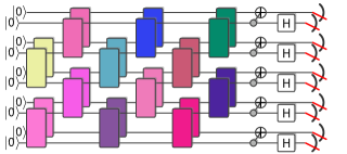
Figure 1: The Bell sampling protocol. In the Bell sampling protocol we prepare the quantum state $C\ket{0^{n}}\otimes C\ket{0^{n}}$ using a quantum circuit $C$, and measure all qubits transversally in the Bell basis across the bipartition of the system.

We begin by defining the Bell sampling protocol and noting some simple properties that will be useful in the remainder of this work. Consider a quantum circuit $C$ acting on $n$ qubits, and define the Bell basis of two qubits as

$$\ket{\sigma_{r}} =(\sigma_{r}\otimes\mathbbm{1})\ket{\Phi^{+}},\text{ where }\ket{\Phi^{+}}=(\ket{00}+\ket{11})/\sqrt{2},$$ (1)

and for $r\in\{0,1\}^{2}$ we identify

$$\sigma_{00}=\mathbbm{1},\quad\sigma_{01}=X,\quad\sigma_{10}=Z,\quad\sigma_{11}=\mathrm{i}\,\sigma_{01}\sigma_{10}=Y.$$ (2)

The Bell sampling protocol proceeds as follows, see Fig. 1.

1. Prepare $\ket{\mathcal{C}}\coloneqq\ket{C}\otimes\ket{C}\coloneqq C\ket{0^{n}}\otimes C\ket{0^{n}}$.

2. Measure all qubit pairs $(i,i+n)$ for $i\in[n]\coloneqq\{1,2,\ldots,n\}$ in the Bell basis, yielding an outcome $r\in\{0,1\}^{2n}$.

It is easy to see that the distribution of the outcomes $r$ can be written as

$$P_{C}(r) =\frac{1}{2^{n}}\left|\bra{C}\sigma_{r}\ket{\overline{C}}\right|^{2}$$ (3)

where $\sigma_{r}=\sigma_{r_{1}r_{n+1}}\otimes\sigma_{r_{2}r_{n+2}}\otimes\cdots\otimes\sigma_{r_{n}r_{2n}}$ is the $n$-qubit Pauli matrix corresponding to the outcome $r=(r_{1},r_{2},\ldots,r_{2n})$, and $\overline{C}$ denotes complex conjugation of $C$. In order to perform the measurement in the Bell basis, we need to apply a depth-1 quantum circuit consisting of $n$ transversal cnot-gates followed by Hadamard gates on the control qubits and a measurement of all qubits in the computational basis.

Our first observation is that Bell sampling is a universal model of quantum computation. In particular, we show that Bell sampling from random circuits is classically intractable under certain complexity-theoretic assumptions. At the same time, we also show that we can use the very same samples to efficiently infer properties of and detect errors in the state preparation. The Bell samples can thus simultaneously be used for quantum computation and act as a classical shadow of the quantum state preparation that may be used to characterize a quantum device.

Computational complexity.

We first show that Bell sampling is a universal model of quantum computation. To show this, we observe that we can estimate both the sign and the magnitude of $\bra{C}Z\ket{C}$ for any quantum circuit $C$ from Bell samples from a circuit $C^{\prime}(C)$ in which we use a variant of Ramsey interferometery with a single ancilla qubit in each copy of the circuit, see the Supplementary Material (SM) [suppmat]. We then show that approximately sampling from the Bell sampling distribution $P_{C}$ is classically intractable on average for universal random quantum circuits $C$ with $\Omega(n^{2})$ gates in a brickwork architecture (as depicted in Fig. 1), assuming certain complexity-theoretic conjectures are satisfied, via a standard proof technique, see the SM [suppmat] for details. The argument puts the complexity-theoretic evidence for the hardness of Bell sampling from random quantum circuits in linear depth on a par with that for standard universal circuit sampling [boixo_characterizing_2018, bouland_complexity_2019, movassagh_quantum_2020, kondo_quantum_2022, krovi_average-case_2022, arute_quantum_2019].

Bell samples as classical circuit shadows.

Samples in the computational basis—while difficult to produce for random quantum circuits—yield very little information about the underlying quantum state. In particular, the problem of verification is essentially unsolved since the currently used methods require exponential computing time. In contrast, from the Bell samples, we can efficiently infer many properties of the quantum state preparation $\ket{C}\otimes\ket{C}$. Known examples include the overlap $\tr[\rho\sigma]$ of a state preparation $\rho\otimes\sigma$ via a swap test, the magic of the state $\ket{C}$ [haug_scalable_2023], and the outcome of measuring any Pauli operator $P\otimes P$ [gottesman_introduction_2009]. Here, we add two new properties to this family. We give efficient protocols for testing the depth of low-depth quantum circuits, for testing its magic, and for learning quantum states that can be prepared by a circuit with low $T$-count.

Let us begin by recapping how a swap test can be performed using the Bell samples, and observing some properties that are useful in the context of benchmarking random quantum circuits. To this end, write the two-qubit swap operator $\mathbb{S}=P_{\bigvee^{2}}-P_{\bigwedge^{2}}$ as the difference between the projectors onto the symmetric subspace $P_{\bigvee^{2}}=\ket{\sigma_{00}}\bra{\sigma_{00}}+\ket{\sigma_{01}}\bra{\sigma_{01}}+\ket{\sigma_{10}}\bra{\sigma_{10}}$ and the antisymmetric subspace $P_{\bigwedge^{2}}=\ket{\sigma_{11}}\bra{\sigma_{11}}$. The overlap $\tr[\rho\sigma]=\tr[(\rho\otimes\sigma)\mathbb{S}]$ can then be directly estimated up to error $\epsilon$ from $M\in O(1/\epsilon^{2})$ Bell samples as

$$\frac{1}{M}\left(|\{r:\pi_{Y}(r)=0\}|-|\{r:\pi_{Y}(r)=1\}|\right).$$ (4)

For quantum state preparations $\rho\otimes\rho$, the overlap quantifies the purity $\tr[\rho^{2}]$ of $\rho$. Using randomized compiling implemented independently on two copies of a fixed circuit, we can convert experimentally relevant noise on the two copies into an effective Pauli channel [wallman_noise_2016, winick_concepts_2022]. Errors also decohere into Pauli channels in repeated rounds of syndrome extraction in stabilizer codes [beale_quantum_2018, huang_performance_2019]. At low noise rates $\eta\ll 1$ we can then approximate $\rho\approx(1-\eta)\ket{C}\bra{C}+\eta\sigma$, and a simple calculation shows that the purity can be used to estimate the fidelity from the relation $1-\tr[\rho^{2}]=2(1-F)+O(\eta^{2})$, where $F=\bra{C}\rho\ket{C}$. Moreover, in the case of random circuits, there is an exact mapping between average fidelity and purity for any noise rate; see the SM [suppmat] for details.

We can compare this to other means of estimating the fidelity of a quantum state. One method that has been widely used recently is cross-entropy benchmarking (XEB), which uses only classical samples from computational-basis measurements [arute_quantum_2019, choi_preparing_2023]. This method can yield reliable estimates of the fidelity of the underlying quantum state under a weaker version of the white-noise approximation [arute_quantum_2019, dalzell_random_2021]. But while Bell sampling is computationally and sample efficient, XEB requires computation of ideal output probabilities of $C$, making it infeasible for already moderate numbers of qubits. Another means for fidelity estimation, shadow fidelity estimation [huang_predicting_2020, kliesch_theory_2021], requires implementing deep Clifford circuits and is only practical for specific states such as stabilizer states [ringbauer_verifiable_2023]. In the SM [suppmat], we also discuss the relation of Bell sampling to other means of verifying quantum computations.

In the following, we will assume that the purity test has succeeded, and resulted in a value close to unity.

Depth test.

We now describe a Bell sampling protocol to measure the depth of a quantum circuit $C$ which is promised to be implemented in a fixed architecture, i.e., with gates applied in layers according to a certain pattern. The basic idea underlying the depth test is to use swap tests on subsystems of different sizes in order to obtain estimates of subsystem purities. For a subsystem $A$ of $[n]$, the subsystem purity is given by $P_{A}(\rho)=\tr[\rho_{A}^{2}]$, where $\rho_{A}=\tr_{A^{c}}[\rho]$ is the reduced density matrix on subsystem $A\subset[n]$. It can be estimated from the fraction of outcome strings with even $Y$-parity $\pi_{Y}(r_{A})$ on the substrings $r_{A}=(r_{i},r_{n+i})_{i\in A}$.

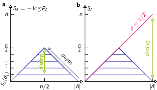
Figure 2: Depth-dependent Page curves. (a) The maximal subsystem entanglement entropy depends on the circuit architecture and depth (shades of blue) until the half-cut entanglement reaches its maximal value given by $n/2$. We measure the subsystem entropy at half-cuts to obtain the maximal sensitivity to different circuit depths. (b) We detect errors in the Bell samples by detecting strings that lead to a non-zero estimate of the purity of $\rho$.

Our test is based on the observation that the amount of entanglement generated by quantum circuits on half-cuts reaches a depth-dependent maximal value until it saturates at a circuit depth that depends on the dimensionality of the circuit architecture, see Fig. 2(a) for an illustration. In order to lower-bound the depth of a circuit family we choose a subsystem size at which the distinguishability between different depths is maximal. This is typically the case at half-cuts, where the Rényi-$2$ entanglement entropy $S_{A}(\rho)=-\log P_{A}(\rho)$ can be at most $n/2$. At the same time, the entanglement entropy is bounded as a function of depth $S_{A}(d)\leq d|\partial A|$, where $\partial A$ is the number of gates applied across the boundary of $A$ in every layer of the circuit. We now compute an empirical estimate $\hat{S}_{n/2}$ of $S_{A}(\ket{C}\bra{C})$ for a size-$n/2$ subsystem $A$ using the Bell samples. In order to obtain a lower bound on the depth of the circuit $C$ generating a given set of Bell samples, we compute the maximum $d$ such that $\hat{S}_{n/2}-\epsilon\geq d\cdot|\partial A|$ up to an error tolerance $\epsilon$ depending on the number of Bell samples. We can further refine this test for random quantum circuits by exploiting their average subsystem entanglement properties, known as the Page curve [page_average_1993]. Depth-dependent Page curves have been computed analytically [nahum_quantum_2017] and numerically [sommers_crystalline_2023] for a few circuit architectures and random ensembles.

We remark that these entanglement-based tests rely on universal features of quantum chaotic dynamics. As a result, they are also expected to be applicable to generic Hamiltonian dynamics, similar to how ideas for standard quantum random sampling have recently been extended to this case [Mark23, Shaw23].

Magic test and Clifford+$T$ learning algorithm.

Another primitive that can be exploited in property tests of quantum states using the Bell samples is the fact that for stabilizer states $\ket{S}$, the Bell distribution is supported on a coset of the stabilizer group of $\ket{S}$ [montanaro_learning_2017]. Leveraging this property allows for efficiently learning stabilizer states [montanaro_learning_2017], testing stabilizerness [gross_schurweyl_2021], learning circuits with a single layer of $T$-gates [lai_learning_2022] and estimating measures of magic [haug_scalable_2023, haug_efficient_2023]. Here, we describe a simple, new protocol that, from the Bell samples, allows us to efficiently estimate the stabilizer nullity, a magic monotone [beverland_lower_2020], and learn states that can be prepared by quantum circuits with $t\in O(\log n)$ $T$-gates.

Our learning algorithm proceeds in two steps. In the first step, we find a compression of the non-Clifford part of the circuit, similarly to Refs. [arunachalam_parameterized_2022, leone_learning_2023-1]. To achieve this, using Bell difference sampling [gross_schurweyl_2021], we find a Clifford unitary $U_{C}$ corresponding to a subspace $C\subset\mathbb{F}_{2}^{2n}$ such that $U_{C}\ket{\psi}$ has high fidelity with $\ket{x}\ket{\varphi}$ for some computational-basis state $\ket{x}$ on the first $\dim(C)$ qubits, and a state $\ket{\varphi}$ on the remaining qubits containing the non-Clifford information. The dimension of $C$ satisfies $\dim(C)\geq n-t$. The number of $T$-gates required to prepare $\ket{\psi}$ is therefore lower-bounded by the stabilizer nullity $M(\ket{\psi})\coloneqq n-\dim(C)$, which is a magic monotone [beverland_lower_2020]. We show that only $O(n/\epsilon)$ Bell samples are sufficient to ensure that $\ket{\psi}$ is $\epsilon$-close to a state with exact stabilizer nullity given by the estimate $\hat{M}$ of $M(\ket{\psi})$. To the best of our knowledge this is the most efficient way of measuring the magic of a quantum state to date.

In the second step of the learning algorithm, we characterize the state $\ket{\varphi}$ on the remaining $n-\dim(C)\leq t$ qubits using pure-state tomography, for example via the scheme of Ref. [guta_fast_2018], giving an estimate $\ket{\hat{\varphi}}$. The output of the algorithm is then given by a classical description of $\ket{\hat{\psi}}=U_{C}\ket{x}\ket{\hat{\varphi}}$. The learning algorithm runs in polynomial time and succeeds with high probability in learning an $\epsilon$-approximation to $\ket{\psi}$ in fidelity using $O(n/\epsilon)$ Bell samples and $O(2^{t}/\epsilon^{2})$ measurements to perform tomography of $\ket{x}\ket{\hat{\varphi}}$.

Using Clifford+$T$ simulators [e.g. bravyi_simulation_2019-1, pashayan_fast_2022, campbell_unified_2017] we can now produce samples from and compute outcome probabilities of $\ket{\hat{\psi}}$ in time $O(2^{t})$. We note that the exponential scaling in $t$ is asymptotically optimal since the description of a state with stabilizer nullity $t$ has $2^{t}+n-t$ real parameters. Our algorithm generalizes to arbitrary non-Clifford gates.

To summarize, we have given efficient ways to extract properties of the circuit $C$—its depth and an efficient circuit description for circuits with low $T$-count—using only a small number of Bell samples. Further properties of $\ket{C}$ that can be efficiently extracted from the Bell samples include the expectation values of any diagonal two-copy observables $A=\sum_{r}a_{r}\ket{\sigma_{r}}\bra{\sigma_{r}}$ and different measures of magic [haug_scalable_2023]. The Bell samples thus serve as an efficient classical shadow of $C$.

Error Detection and Correction

In the last part of this paper, we discuss another appealing feature of Bell samples: we can perform error detection and correction. The idea that redundantly encoding quantum information in many copies of a quantum state allows error detection goes back to the early days of quantum computing. Already in 1996, barenco_stabilisation_1996 have shown that errors can be reduced by symmetrizing many copies of a noisy quantum state. More recently Refs. [cotler_quantum_2019, koczor_exponential_2021, huggins_virtual_2021] used measurements on multiple copies to suppress errors in expectation value estimation. In our two-copy setting, some simple single-sample error detection properties follow immediately from the tests in the previous section.

First, we observe that an outcome in the antisymmetric subspace, i.e., an outcome $r$ with $\pi_{Y}(r)=1$, is certainly due to an error. We can thus reduce the error in the sampled distribution by discarding such outcomes. We show in the SM [suppmat] that such error detection reduces the error rate of a white-noise model by approximately a factor of $2$. Quantum computations in the Bell sampling model with error detection can thus achieve equal fidelities to circuit model computations, where no error detection is possible, in spite of the factor of 2 in qubit overhead.

Second, we note that Bell samples are compatible with stabilizer codes. For such codes, the Bell measurement between code blocks is a transversal measurement, and allows to extract the syndrome $\sigma\otimes\sigma$ for $\sigma\in\mathsf{P}_{n}$ in the stabilizer of the code [gottesman_introduction_2009]. If a detectable/correctable error occurred in one of the code blocks, this syndrome detects/identifies that error up to stabilizer equivalence. The fact that the Bell measurement is transversal implies that an error in the Bell measurement does not spread, so that local error channels or coherent errors in the entangling cnot gates in the Bell measurement reduce the overall measurement fidelity by $(1-\epsilon)^{n}$, where $\epsilon$ is the error rate per Bell pair. Bell sampling is thus feasible in the regime of $\epsilon\ll 1/n$. We also note that antisymmetric errors in the Bell measurement are detectable.

Finally, we observe that quadratic error suppression is possible for estimating the expectation values of diagonal two-copy observable $A$, through the estimate $\tr[A\rho^{\otimes 2}]/\tr[\mathbb{S}\rho^{\otimes 2}]$, similar to virtual distillation [cotler_quantum_2019, huggins_virtual_2021, koczor_exponential_2021]. Specifically, this is true for estimating the expectation $\bra{E_{0}}P\ket{E_{0}}^{2}$ of a Pauli observable $P$ in the ground state $\ket{E_{0}}$ of a gapped Hamiltonian by choosing $A=(P\otimes P)\mathbb{S}$, see the SM [suppmat] for details.

Discussion and outlook.

In this work, we have considered Bell sampling as a model of quantum computation. We have shown that many properties of the quantum circuit preparing the underlying state can be extracted efficiently, and that in particular certain errors in the state preparation can be detected from single shots. Based on this, we have argued that the Bell samples act as classical circuit shadows. Since Bell sampling is universal this allows us to perform universal quantum computations whose outputs also yield information about the quantum circuit. This makes Bell sampling an interesting computational model, and our main focus in this work is to establish this fact.

We leave it as an open question how much overhead is required when performing computations with Bell sampling. While our -completness proof requires an additional ancilla qubit, it is conceivable, that one can encode an $n$-qubit computation in the circuit model using two copies of an $m$-qubit system with $m\leq n$ via Bell sampling.

Bell sampling is not only interesting conceptually, however. It is also realistic. Since the Bell basis measurement requires only transversal cnot and single-qubit gates, it can be naturally implemented in unit depth on various quantum processor architectures with long-range connectivity. These include in particular ion traps [bermudez_assessing_2017] and Rydberg atoms in optical tweezers [bluvstein_quantum_2022]. It is more challenging to implement Bell sampling in geometrically local architectures such as superconducting qubits [arute_quantum_2019]. In such architectures, one can interleave the two copies in a geometrically local manner such that the Bell measurement is a local circuit; however, this comes at the cost of additional layers of SWAP gates for every unit of circuit depth. Alternatively, one can use looped pipeline architectures to implement the Bell measurement [Cai2022].

But is Bell sampling also practical in the near term? To satisfactorily answer this question, various sources of noise need to be analyzed in detail—tasks we defer to future work but mention here. For some of our protocols, including the purity test and the error detection protocols we discuss the effect of noise sources on the state preparation. But how severely does measurement noise affect the outcomes? In other instances, including the depth and magic test, and the low-$T$ count learning algorithms we have restricted ourselves to (nearly) pure state preparations. We can at least certify that these algorithms are applicable because the purity of the state preparation can be independently checked. But in currently realistic scenarios, the state preparation of deep circuits will never be pure. An important question is therefore whether we can formulate noise-robust versions of these protocols.

While we have exploited the purity of the state $\ket{C}$ in our error detection protocol, it is in an interesting question whether it is possible to detect additional errors from the Bell samples. For instance, it might be possible to exploit the fact that the subsystem purity of the target state is low for large subsystems, see Fig. 2.

We have shown that classically simulating the Bell sampling protocol with universal random circuits is classically intractable. An exciting question in this context is whether the complexity of Bell sampling might be more noise robust than computational-basis sampling in the asymptotic scenario. For universal circuit sampling in the computational basis gao_efficient_2018, aharonov_polynomial-time_2022 developed an algorithm that simulates sufficiently deep random circuits with a constant noise rate in polynomial time. In the Supplementary Material [suppmat] we give some initial evidence that this simulation algorithm fails for Bell measurements. If the hardness of Bell sampling indeed turns out to be robust to large amounts of circuit noise, we face the exciting prospect of a scalable quantum advantage demonstration with classical validation and error mitigation.

Note: While finalizing this work, we became aware of Refs. [grewal_efficient_2023-2, leone_learning_2023], where the authors independently report algorithms similar to the one we present above for learning quantum states generated by circuits with low $T$-count. After this work was completed, we collaborated on the physical implementation of Bell sampling in a logical qubit processor, illustrating the feasibility of our results to near-term devices [bluvstein_logical_2023].

Acknowledgements

D.H. warmly thanks Abhinav Deshpande and Ingo Roth for helpful discussions that aided in the proofs of Lemma 2 and Lemma 4, respectively. We are also grateful to Dolev Bluvstein, Maddie Cain, Bill Fefferman, Xun Gao, Soumik Ghosh, Alexey Gorshkov, Vojtěch Havlíček, Markus Heinrich, Marcel Hinsche, Marios Ioannou, Marcin Kalinowski, Mikhail Lukin and Brayden Ware for discussions. This research was supported in part by NSF QLCI grant OMA-2120757 and Grant No. NSF PHY-1748958 through the KITP program on “Quantum Many-Body Dynamics and Noisy Intermediate-Scale Quantum Systems.” D.H. acknowledges funding from the US Department of Defense through a QuICS Hartree fellowship.

Supplementary Material for “Bell sampling from quantum circuits”
Dominik Hangleiter and Michael J. Gullans

S1 -completeness of Bell sampling

In this section, we show that Bell sampling is -complete as a model of quantum computation in spite of the fact that we are restricting to circuits of the form $C\otimes C$ and measurements in the transversal Bell basis.

Lemma 1 (-completeness).

Bell sampling is -complete.

Proof.

Consider an arbitrary quantum circuit $C$. Then estimating the probability of measuring the first qubit of $C$ in the $\ket{1}$ state up to additive precision is -complete. The idea of the proof is to design a circuit $C^{\prime}$ such that we can infer $p_{1}\coloneqq\tr[(\ket{1}\bra{1}\otimes\mathbbm{1}_{n-1})C\ket{0^{n}}\bra{0^{n}}C^{\dagger}]$ from Bell samples from $C^{\prime}$. Let $\rho=\tr_{[n]\setminus\{1\}}[C\ket{0^{n}}\bra{0^{n}}C^{\dagger}]$ be the reduced density matrix of the first qubit of the state $C\ket{0}$ before the measurement. Then our task is to estimate $p_{1}=\tr[\rho\ket{1}\bra{1}]$ from Bell sampling.

To achieve this, we make use of the fact that we can infer the square of any Pauli expectation value $\bra{C}P\ket{C}^{2}$ up to additive precision from Bell samples from $\ket{C}\otimes\ket{C}$ for any circuit $C$. Starting from an arbitrary quantum circuit $C$ we add an ancillary qubit (labeled by $0$) before the first qubit and run the circuit $C^{\prime}=\mathrm{e}^{-\mathrm{i}\frac{\pi}{8}(Z_{0}Z_{1}+Z_{0})}(H\otimes C)$, where $H$ denotes the Hadamard gate. The resulting marginal state on the ancillary qubit is then given by

$$\tr_{[n]}[\mathrm{e}^{-\mathrm{i}\frac{\pi}{8}(Z_{0}Z_{1}+Z_{0})}(\ket{+}\bra{+}\otimes\rho)\mathrm{e}^{\mathrm{i}\frac{\pi}{8}(Z_{0}Z_{1}+Z_{0})}\\ =\frac{1}{2}\left(\mathbbm{1}+\left(\frac{1}{2}-\frac{1}{2}\bra{C}Z_{1}\ket{C}\right)X+\left(\frac{1}{2}+\frac{1}{2}\bra{C}Z_{1}\ket{C}\right)Y\right).$$ (S1)

From Bell samples from $\ket{C^{\prime}}\otimes\ket{C^{\prime}}$ we can now estimate $|\bra{C^{\prime}}X_{0}\ket{C^{\prime}}|=|1-\bra{C}Z_{1}\ket{C}|/2=p_{1}$. ∎

S2 Classical hardness of Bell sampling

In this section, we provide complexity-theoretic evidence that sampling from the Bell distribution $P_{C}$ up to constant total-variation distance (TVD) error is classically intractable.

In order to show this, we follow a standard proof strategy, which has three main ingredients.

1. Hiding: The distributions over outcomes and circuit instances are interchangeable.

2. Average-case  hardness of approximating the output probabilities. While we cannot prove this in any instance, we typically provide evidence for it using three ingredients:

   1. Worst-case  hardness of approximation,

   2. Average-case  hardness of near-exact computation, and

   3. Anticoncentration.

We defer the reader to Section III of Ref. [hangleiter_computational_2023-1] for a detailed exposition of the proof strategy.

S2.1 Hiding

Consider the Bell sampling distribution

$$P_{C}(r) =\frac{1}{2^{n}}|\bra{\sigma_{r}}C\otimes C\ket{0^{2n}}|^{2}$$ (S2)

$$=\frac{1}{2^{n}}|\bra{\Phi^{+}}(\sigma_{r}\otimes\mathbbm{1})(C\otimes C)\ket{0^{2n}}|^{2}.$$ (S3)

Then, using that $\ket{\Phi^{+}}=\operatorname{vec}(\mathbbm{1})/{\sqrt{2}}$, we find that

$$(\sigma_{r}\otimes\mathbbm{1})\ket{\Phi^{+}}=(\sqrt{\sigma_{r}}\otimes\sqrt{\sigma_{r}}^{T})\ket{\Phi^{+}},$$ (S4)

and hence

$$P_{C}(r)=|\bra{\Phi^{+}}\sqrt{\sigma_{r}}C\otimes\sqrt{\sigma_{r}}^{T}C\ket{0^{2n}}|^{2},$$ (S5)

so that for $x$ such that $\sqrt{\sigma_{r}}\neq\sqrt{\sigma_{r}}^{T}$, we cannot write $P_{C}(r)=P_{C}^{\prime}(0^{n})$ for some $C^{\prime}=C^{\prime}(C,r)$. And indeed, while $\sqrt{X}^{T}=\sqrt{X}$ and $\sqrt{Z}^{T}=\sqrt{Z}$, we have $\sqrt{Y}^{T}\neq\sqrt{Y}$.

This means that hiding does not hold on the full output distribution. However, we can restrict ourselves to the a priori known support of the Bell sampling distribution, which is given by the symmetric subspace, characterized by $\pi_{Y}(r)=0$. Indeed, we can view the fact that $\sqrt{Y}^{T}\neq\sqrt{Y}$ as a signature of the fact that the corresponding Bell state is not symmetric. Conversely, consider an even number of $Y$-outcomes. Specifically, for a two-qubit state with two $Y$-outcomes, we can explicitly check that $\sqrt{Y\otimes Y}^{T}=\sqrt{Y\otimes Y}$.

Hence, hiding holds on the symmetric subspace for any architecture that includes a layer of single-qubit gates that is invariant under $\sqrt{X},\sqrt{Y},\sqrt{Z}$ at the end of the circuit.

Furthermore, defining $C_{r}=\sqrt{\sigma_{r}}C$ we observe that

$$|\bra{\sigma_{r}}C_{s}\ket{0^{2n}}|^{2}=|\bra{\sigma_{r\oplus s}}C\ket{0^{2n}}|^{2},$$ (S6)

since $\sqrt{\sigma_{r}}\sigma_{s}\sqrt{\sigma_{r}}\in\sf P_{n}$, where $\sf P_{n}$ is the Pauli group with phases in $\{\pm 1,\pm\mathrm{i}\}$.

S2.2 Average-case  hardness of approximating outcome probabilities

S2.2.1 Worst-case  hardness of approximating outcome probabilities

Lemma 2.

Given a quantum circuit $C$, it is -hard to compute $2^{-n}|\bra{C}\sigma_{r}\ket{\overline{C}}|^{2}$ up to relative error $<1/2$.

Proof.

In order to perform the Bell basis measurement we apply $\texttt{cnot}(H\otimes\mathbbm{1})$ across all pairs of qubits. Writing $\ket{C}=\sum_{x}c_{x}\ket{x}$, the pre-measurement state then transforms as

$$\ket{C}\otimes\ket{C}= \sum_{xy}c_{x}c_{y}\ket{x}\ket{y}$$ (S7)

$$\xrightarrow{\texttt{cnot}^{\otimes n}} \sum_{xy}c_{x}c_{y}\ket{x}\ket{x\oplus y}$$ (S8)

$$\xrightarrow{(H\otimes\mathbbm{1})^{\otimes n}} \sum_{xyz}(-1)^{x\cdot z}c_{x}c_{y}\ket{z}\ket{x\oplus y}\eqqcolon\ket{\mathcal{C}}.$$ (S9)

Consider a state $\ket{C}$ on $n+1$ qubits and the $(0^{n}1,0^{n+1})$-Bell amplitude

$$\bra{0^{n}1}\bra{0^{n+1}}\ket{\mathcal{C}} =\sum_{xyz}(-1)^{x\cdot z}c_{x}c_{y}\innerproduct{0^{n}1}{z}\innerproduct{0^{n+1}}{x\oplus y}$$ (S10)

$$=\sum_{x}(-1)^{x\cdot 0^{n}1}c_{x}^{2}$$ (S11)

$$=\sum_{x:x_{n}=0}c_{x}^{2}-\sum_{x:x_{n}=1}c_{x}^{2}.$$ (S12)

Let us now specify $\ket{C}\coloneqq\ket{C_{f}}\propto\sum_{x}\ket{x}\ket{f(x)}$ up to normalization, where $f:\{0,1\}^{n}\rightarrow\{0,1\}$ is an efficiently computable Boolean function. Observe that for $b\in\{0,1\}$

$$(\mathbbm{1}\otimes\bra{b})\sum_{x}\ket{x}\ket{f(x)}=\sum_{x:f(x)=b}\ket{x}.$$ (S13)

For $b=1$ the state (S13) is normalized by the square root of the number of accepting inputs of $f$, given by $\#f\coloneqq|\operatorname{Acc}(f)|\equiv|\{x:f(x)=1\}|$, and for $b=0$ by $\sqrt{2^{n}-\#f}$ . Hence, the coefficients of $\ket{C_{f}}=\sum_{x\in\{0,1\}^{n+1}}c_{x}\ket{x}$ are given by

$$c_{yb}\equiv(\bra{y}\otimes\bra{b})\ket{C_{f}}=\begin{cases}1/\sqrt{\#f},&f(y)=b=1\\ 1/\sqrt{2^{n}-\#f},&f(y)=b=0\\ 0&\text{otherwise}.\end{cases}$$ (S14)

Let us now add another qubit so that we have $n+2$ qubits in total. Given an arbitrary efficiently computable Boolean function $g:\{0,1\}^{n}\rightarrow\{0,1\}$ let us define

$$f_{g} :\{0,1\}^{n+1}\rightarrow\{0,1\}$$ (S15)

$$f_{g}(y)=\begin{cases}1&\text{ if }y=(x,g(x))\\ 0&\text{ if }y=(x,\neg g(x)).\end{cases}$$ (S16)

We now reversibly compute the function $f_{g}$ obtaining $n+2$-bit outcome strings $(y,f_{g}(y))$ with the property that $f_{g}(y)=1$ if $y=(x,g(x))$. So the $(n+1)$st qubit encodes the outcome of $g$ while the last (i.e., $(n+2)$nd) qubit encodes the outcome of $f_{g}$.

$f_{g}$ can be efficiently computed: Let $D$ be the circuit that maps $\ket{x}\ket{b}\rightarrow\ket{x}\ket{g(x)\oplus b}$. Then the quantum circuit $C=(\mathbbm{1}_{n}\otimes\texttt{cnot}(X\otimes\mathbbm{1}))(D^{\dagger}\otimes\mathbbm{1})$ computes $\ket{y}\ket{0}\mapsto\ket{y}\ket{f_{g}(y)}$.

We observe that

$$|\operatorname{Acc}(f_{g})|=|\operatorname{Rej}(f_{g})|=2^{n+1}/2$$ (S17)

and, moreover, we have

$$|\operatorname{Acc}(g)|=|\{y\in\operatorname{Acc}(f_{g}),y_{n}=1\}| =|\{y\in\operatorname{Rej}(f_{g}),y_{n}=0\}|,$$ (S18)

$$|\operatorname{Rej}(g)|=|\{y\in\operatorname{Acc}(f_{g}),y_{n}=0\}| =|\{y\in\operatorname{Rej}(f_{g}),y_{n}=1\}|.$$ (S19)

To see the latter, just observe that

$$|\{y\in\operatorname{Acc}(f_{g}),y_{n}=1\}|=|\{(x,g(x)):g(x)=1\}|\\ =|\{(x,\neg g(x)):\neg g(x)=0\}|=|\operatorname{Acc}(g)|.$$ (S20)

Let us consider the outcome string $(0^{n}11,0^{n+2})$ and compute the corresponding amplitude of the state $\ket{\mathcal{C}_{f_{g}}}=((H\otimes\mathbbm{1})\cdot\texttt{cnot})^{\otimes(n+2)}\ket{C}\otimes\ket{C}$ as

$$\bra{0^{n}11,0^{n+2}}\ket{\mathcal{C}_{f_{g}}} =\sum_{xyz}(-1)^{x\cdot z}c_{x}c_{y}\innerproduct{0^{n}11}{z}\innerproduct{0^{n+2}}{x\oplus y}$$ (S21)

$$=\sum_{x}(-1)^{x\cdot(0^{n}11)}c_{x}^{2}$$ (S22)

$$=\sum_{x:x_{n}=0,x_{n+1}=0}c_{x}^{2}-\sum_{x:x_{n}=1,x_{n+1}=0}c_{x}^{2}-\sum_{x:x_{n}=0,x_{n+1}=1}c_{x}^{2}+\sum_{x:x_{n}=1,x_{n+1}=1}c_{x}^{2}$$ (S23)

$$\stackrel{{\scriptstyle\eqref{eq:equality fg}}}{{=}} \frac{1}{2^{n}}\left(|\{y\in\operatorname{Rej}(f_{g}):y_{n}=0\}|-|\{y\in\operatorname{Rej}(f_{g}):y_{n}=1\}|\right)$$ (S24)

$$\quad+\frac{1}{2^{n}}\left(|\{y\in\operatorname{Acc}(f_{g}):y_{n}=1\}|-|\{y\in\operatorname{Acc}(f_{g}):y_{n}=0\}|\right)$$ (S25)

$$\stackrel{{\scriptstyle\eqref{eq:equality g}}}{{=}} \frac{2}{2^{n}}\left(|\operatorname{Acc}(g)|-|\operatorname{Rej}(g)|\right)\equiv\frac{1}{2^{n-1}}\operatorname{gap}(g)$$ (S26)

This shows that the output amplitudes of Bell sampling from universal quantum circuits can encode the gap of any -function. Finally, we reduce the outcome to the all-zero outcome—and by the hiding property any outcome in the symmetric subspace—by observing that the output string corresponds to the $\ket{\mathbbm{1}}^{\otimes n}\ket{Z}^{\otimes 2}$ outcome and hence we can define $\tilde{C}_{f_{g}}=(\mathbbm{1}^{\otimes n}\otimes(Z^{1/2})^{\otimes 2})C_{f_{g}}$ to show that $\bra{0^{2(n+2)}}\ket{\mathcal{C}_{f_{g}}}$ is -hard to compute.

By Proposition 8 of bremner_average-case_2016 (see also Lemma 8 of Ref. [hangleiter_computational_2023-1]), approximating $|\bra{0^{2n}}\ket{\tilde{\mathcal{C}}_{f_{g}}}|^{2}$ up to any relative error $<1/2$ or additive error $1/2^{2(n+1)}$ is -hard. ∎

Notice that this argument also proves that computing certain Pauli coefficients of an $n$-qubit quantum circuit is  hard up to relative error $<1/2$ since the circuit $C_{f_{g}}$ we have used in the encoding of the gap of a  function is real and $|\bra{C}\sigma_{r}\ket{\overline{C}}|^{2}=|\tr[\ket{C}\bra{C}\sigma_{r}]|^{2}$ for a real circuit $C$. Notice, however, that we cannot reduce to the all-zero string in this case. This is also easy to see since the probability of the all-zero outcome of a real circuit is always one.

Conversely, if we include the $\sqrt{Z}\otimes\sqrt{Z}$ gate at the end of $C_{f_{g}}$, this shows that computing the overlap $|\bra{C}\ket{\overline{C}}|^{2}$ is -hard in general.

The next step in applying the Stockmeyer argument is to see if approximate average-case hardness is plausible. To this end we can/need to make two arguments.

S2.2.2 Near-exact average-case hardness

First, we need to show (near-)exact average-case hardness, see [hangleiter_computational_2023-1, Sec. IV.D.5] for the available techniques.

Consider a circuit $C$ with some Haar-random 2-qubit gates. Let us follow the strategy by krovi_average-case_2022. Analogously, we interpolate every 2-qubit gate $G_{i}$ in the worst-case circuit $C$ to a Haar random gate $H_{i}G_{i}$ with $H_{i}$ drawn from the 2-qubit Haar measure.

$$G_{i}(\theta) =\exp(\mathrm{i}(1-\frac{\theta}{2m})\log H_{i})G_{i}$$ (S27)

$$=V_{i}^{\dagger}\sum_{k_{i}=1}^{4}\mathrm{e}^{\mathrm{i}(1-\frac{\theta}{2m})\phi_{k_{i}}}\ket{\psi_{k_{i}}}\bra{\psi_{k_{i}}}V_{i}G_{i}$$ (S28)

$$\eqqcolon\sum_{k_{j}}\mathrm{e}^{\mathrm{i}(1-\frac{\theta}{2m})\phi_{k_{i}}}\tilde{G}_{k_{j}}$$ (S29)

where $V_{i}$ diagonalizes $H_{i}$ into eigenvectors $\ket{\psi_{k_{i}}}$ and eigenvalues $\exp(\mathrm{i}\phi_{k_{i}})$. Notice that compared to krovi_average-case_2022, we interpolate only by an angle $\theta/2m$ instead of $\theta/m$. Now, we consider the circuit $C(\theta)$ defined by replacing all the gates $G_{i}$ of $C$ with $G_{i}(\theta)$. We can write the output probability as

$$|\bra{0^{2n}}\ket{\mathcal{C}(\theta)}|^{2}=|\bra{\Phi^{+}}^{\otimes n}C(\theta)\otimes C(\theta)\ket{0^{2n}}\\ =\left|\sum_{k_{ij}:i\in[m],j\in\{0,1\}}\mathrm{e}^{\mathrm{i}(1-\frac{\theta}{2m})\sum_{ij}\phi_{k_{ij}}}\bra{\Phi^{+}}^{\otimes n}\tilde{G}_{k_{00}}\cdots G_{k_{d1}}\ket{0^{2n}}\right|^{2}\\ =\sum_{k,k^{\prime}}\mathrm{e}^{\mathrm{i}(1-\frac{\theta}{2m})\Delta\phi_{k,k^{\prime}}}\bra{\Phi^{+}}\tilde{G}_{k}\ket{0}\bra{0}\tilde{G}_{k}^{\dagger}\ket{\Phi^{+}},$$ (S30)

where $k=(k_{00},k_{01},\ldots,k_{m1})$, $\tilde{G}_{k}=\prod_{ij}G_{k_{ij}}$ and $\Delta\phi_{k,k^{\prime}}=\sum_{ij}(\phi_{k_{ij}}-\phi_{k^{\prime}_{ij}})$. Since $|\Delta\Phi_{k,k^{\prime}}|/2m\in O(1)$, we can now follow the argument of Krovi, replacing $m\leftarrow 2m$, to construct a polynomial of degree $d\in O(m/\log(m)^{2})$ that approximates the output probabilities of Bell sampling. Using this polynomial, we can run robust polynomial interpolation to obtain near-exact average-case hardness.

S2.2.3 Anticoncentration

Finally, the question arises whether the output distribution anticoncentrates. Recall that anticoncentration is defined as

$$\Pr_{C\sim\mathcal{C}}\left[P_{C}(S)\geq\frac{1}{|\Omega|}\right]\geq\gamma,$$ (S31)

for constant $\gamma$ and the sample space $\Omega$. Our standard tool for showing anticoncentration is the Payley-Zygmund inequality which lower bounds the anticoncentrating fraction in terms of second moments as

$$\Pr_{C\sim\mathcal{C}}\left[Z\geq\alpha\mathbb{E}[Z]\right]\geq(1-\alpha)^{2}\frac{\mathbb{E}[Z]^{2}}{\mathbb{E}[Z^{2}]},$$ (S32)

for a random variable $Z$ with $0\leq Z\leq 1$ which we take to be $Z=P_{C}(S)$.

This problem gets interesting for the Bell sampling circuits since already a single copy of the Bell sampling state has two copies of the circuit, so we will need second and fourth moments of the circuit family to show anticoncentration with the standard technique. Recall that the Bell sampling output distribution is given by

$$P_{C}(r)=|\bra{\sigma_{x}}C\otimes C\ket{0^{2n}}|^{2},$$ (S33)

where $\sigma_{r}=\prod_{i=1}^{N}\sigma_{x_{i}}$. Let’s assume that we have a four-design and begin with the first moment.

$$\mathbb{E}[P_{C}(r)] =\bra{\sigma_{r}}\mathbb{E}\left[C\otimes C\ket{0^{2n}}\bra{0^{2n}}C^{\dagger}\otimes C^{\dagger}\right]\ket{\sigma_{r}}$$ (S34)

$$=\frac{1}{D_{[2]}}\bra{\sigma_{r}}P_{[2]}\ket{\sigma_{r}},$$ (S35)

where $D_{[t]}=\binom{d+t-1}{t}$ and $P_{[t]}$ is the projector onto the symmetric subspace of $t$ copies (see [zhu_clifford_2016] for a nice intro). We can explicitly compute the expression as

$$\bra{\sigma_{r}} P_{[2]}\ket{\sigma_{r}}=\frac{1}{2}\bra{\sigma_{r}}(\mathbbm{1}+\mathbb{S})\ket{\sigma_{r}}$$ (S36)

$$=\bra{\Phi^{+}}(\sigma_{r}^{2}\otimes\mathbbm{1})\ket{\Phi^{+}}+\bra{\Phi^{+}}(\sigma_{r}\sigma_{r}^{T}\otimes\mathbbm{1})\ket{\Phi^{+}}$$ (S37)

$$=2^{n}(1+(-1)^{\pi_{Y}(r)}),$$ (S38)

where we in abuse of notation we write $\ket{\Phi^{+}}=\ket{\Phi^{+}}^{\otimes n}$ and observe that $\tr[XX^{T}]=\tr[ZZ^{T}]=\tr[\mathbbm{1}]=2^{n}$ and $\tr[YY^{T}]=-2^{n}$. We find—as expected—that the Bell state with an odd number of singlet states (coresponding to $\sigma_{r}=Y$) is in the antisymmetric subspace and therefore the projector onto the symmetric subspace evaluates to zero in that case:

$$\mathbb{E}[P_{C}(r)]=\begin{cases}D_{[2]}^{-1}=2/(2^{2n}(1+2^{-n}))&\text{if }\pi_{Y}(r)\text{ even}\\ 0&\text{if }\pi_{Y}(r)\text{ odd}\end{cases}.$$ (S39)

The output distribution is thus supported on the even $Y$-parity sector on which all outcomes have equal expectation value given by $D_{[2]}^{-1}=2/(2^{n}(2^{n}+1))$. The size of the even-$Y$-parity sector should be exactly given by this number since these strings correspond to a basis of the symmetric subspace.

The second moment is more complicated. It reads

$$\mathbb{E}[\bra{\sigma_{r}}^{\otimes 2}C^{\otimes 4}\ket{0}\bra{0}(C^{\dagger})^{\otimes 4}\ket{\sigma^{r}}^{\otimes 2}]\\ =\frac{1}{D_{[4]}}\bra{\sigma_{r}}^{\otimes 2}P_{[4]}\ket{\sigma_{r}}^{\otimes 2}$$ (S40)

To compute this overlap on the symmetric subspace on which $\sigma_{r}=\sigma_{r}^{T}$, we write $P_{[f]}=4!^{-1}\sum_{\sigma\in S_{4}}P_{\sigma}$, where $P_{\sigma}$ is the permutation matrix corresponding to the element $\sigma$ of the symmetric group $S_{4}$. We observe that for a $c=1/3$-fraction of the permutations in the definition of $P_{[4]}$ the overlap evaluates to $\tr[\sigma_{r}^{2}]^{2}/2^{2n}=\tr[\mathbbm{1}]^{2}/2^{2n}=1$, while for the other $1-c$ fraction, it evaluates to $\tr[\sigma_{r}^{4}]/2^{2n}=\tr[\mathbbm{1}]/2^{2n}=1/2^{n}$. Viewing the Bell state $\ket{\Phi^{+}}$ as a vectorization of the identity matrix, these correspond exactly to the cases in which there are one versus two connected components in the resulting graph.

Consequently, we find

$$\mathbb{E}[\bra{\sigma_{r}}^{\otimes 2}C^{\otimes 4}\ket{0}\bra{0}(C^{\dagger})^{\otimes 4}\ket{\sigma^{r}}^{\otimes 2}]\\ =\frac{1}{D_{[4]}}\left(c+\frac{1-c}{2^{n}}\right).$$ (S41)

for all even $Y$-parity $r$ (satisfying that $\pi_{Y}(r)$ is even).

From this we find that if $\mathcal{C}$ generates a state $4$-design, for all $r$ in the symmetric subspace

$$\Pr[P_{C}(r)\geq\frac{\alpha}{D_{[2]}}] \geq(1-\alpha)^{2}\frac{1}{c+\frac{1-c}{2^{n}}}\frac{D_{[4]}}{D_{[2]}^{2}}$$ (S42)

$$=\frac{(1-\alpha)^{2}}{3!\cdot(c+\frac{1-c}{2^{n}})}\frac{(2^{n}+3)(2^{n}+2)}{(2^{n}+1)2^{n}}$$ (S43)

$$\geq\frac{(1-\alpha)^{2}}{6c}$$ (S44)

By the result of brandao_local_2016, this means that the Bell sampling distribution anticoncentrates in linear depth. Given the fact that we just copied two random circuits and qualitatively found the same results as for a single copy, we conjecture that the Bell sampling distribution also anticoncentrates in $\log$-depth. To check this, we would have to directly compute the moments of the output distribution, but this becomes more complicated than for the single-copy case. This is because the local degrees of freedom the standard mapping to a statistical-mechanical model [zhou_emergent_2019, hunter-jones_unitary_2019, barak_spoofing_2021, dalzell_random_2022], increase from 2 to 24 permutations.

S3 Learning circuit properties from Bell sampling

In the following, we will detail the tests that can be performed using just the samples from the Bell distribution. Success on those tests—while falling short of loophole-free verification—increases our confidence in the correctness of the experiment.

S3.1 Measuring purity and fidelity

Our first observation is that, given some noisy state preparation $\rho\otimes\sigma$, we can estimate $\tr[\rho\sigma]$ from Bell measurements on $\rho\otimes\sigma$. To see this, observe that we can express the single-qubit swap operator in the Bell basis as

$$\mathbb{S} =\ket{00}\bra{00}+\ket{11}\bra{11}+\ket{01}\bra{10}+\ket{10}\bra{01}$$ (S45)

$$=\underbrace{\ket{\sigma_{00}}\bra{\sigma_{00}}+\ket{\sigma_{01}}\bra{\sigma_{01}}+\ket{\sigma_{10}}\bra{\sigma_{10}}}_{P_{\bigvee^{2}}}-\underbrace{\ket{\sigma_{11}}\bra{\sigma_{11}}}_{P_{\bigwedge^{2}}}$$ (S46)

Hence, we can estimate the overlap

$$O(\rho,\sigma)=\tr[\rho\sigma]=\tr[(\rho\otimes\sigma)\mathbb{S}]$$ (S47)

by taking the difference between the frequency of outcomes with even parity of $11$-outcomes and odd parity of $11$-outcomes

$$\hat{O}=\frac{1}{M}\left(|\{r:\pi_{Y}(r)=0\}|-|\{r:\pi_{Y}(r)=1\}|\right),$$ (S48)

where $M$ is the total number of measurements.

Let us now see what the quantity $O(\rho,\sigma)$ corresponds to for various assumptions on what $\rho$ and $\sigma$ are.

S3.1.1 Purity and Fidelity

The weakest assumption is that $\rho=\sigma$. In this case

$$O(\rho,\rho)=\tr[\rho^{2}]=P(\rho)$$ (S49)

is just the purity of $\rho$.

Using randomized compiling implemented independently on each copy of the Bell sampling circuit, the effective noise channel for the Bell samples can be approximately reduced to a Pauli channel [wallman_noise_2016]. Strictly speaking, randomized compiling works well in the experimentally relevant setting in which there are some ‘easy’ gates, say, Pauli gates, on which the noise is approximately gate-independent and some ‘hard’ gates which have gate-dependent errors. In that setting, the gate-dependent noise on the hard gates, except for those in the last layer of the circuit, can be reduced to a Pauli channel. In this case, the effective density matrix on each copy can approximately be written as

$$\rho_{C}(\eta)\coloneqq(1-\eta)\ket{C}\bra{C}+\eta\,\sigma,$$ (S50)

for another density matrix $\sigma$. As we showed in the main text, when $\eta\ll 1$, the purity can then be used to estimate the fidelity

$$F(\rho_{C}(\eta),\ket{\mathcal{C}}\bra{\mathcal{C}})=1-\eta\big{(}1-\langle C|\sigma|C\rangle\big{)}.$$ (S51)

Generically, we expect that $\bra{C}\sigma\ket{C}$ is exponentially small since after randomized compiling, the deviation $\sigma$ from the ideal state $\ket{C}\bra{C}$ is uncorrelated with $\ket{C}\bra{C}$.

Indeed, a particularly simple realization of this noise model occurs in the so-called white-noise approximation where $\sigma=\mathbbm{1}/2^{n}$. In that case, the correspondence between fidelity and purity holds for any noise rate. From $P(\rho_{C}(\eta))$ we can easily obtain an estimate of $\eta$ since

$$\tr[\rho_{C}(\eta)^{2}]=(1-\eta)^{2}+\eta(1-\eta)/2^{n}+\eta^{2}/2^{2n},$$ (S52)

which lets us directly estimate the fidelity

$$F(\rho_{C}(\eta),\ket{\mathcal{C}}\bra{\mathcal{C}})=1-\eta(1-1/2^{n}).$$ (S53)

S3.1.2 Average fidelity

Finally, following an argument in Ref. [ware_sharp_2023], consider circuits $C$ constructed from two-qubit gates which form a unitary 2-design, and consider the noise setting in which a single-qubit Pauli noise channel $\mathcal{N}=\sum_{i\in\{0,\ldots,3\}}p_{i}\sigma_{i}\cdot\sigma_{i}$ with acts on every qubit after the application of a two-qubit gate. Let $\mathcal{U}=|U\rrangle\llangle U^{\dagger}|\equiv\mathrm{vec}(U\cdot U^{\dagger})$ be the matricization of the adjoint action of the two-qubit gate $U$, where we denote the vectorization of a matrix $A$ by $|A\rrangle$. The full circuit is then composed of two copies of noisy unitary two-qubit channels given by $\mathcal{N}^{\otimes 4}{\mathcal{U}^{\otimes 2}}$, where the cut is across the bipartition of the Bell measurement, and let the noisy state be $\rho(\epsilon)$.

Then, we can express the fidelity between a state with noise rate $\epsilon$ and a state with noise rate $0$, as the purity of a state with noise rate $\epsilon^{\prime}$. To see this, we evaluate the average over gates in a single layer of the circuit. Then

$$\mathbb{E}_{U}\mathcal{N}^{\otimes 4}\mathcal{U}^{\otimes 2}=\sum_{\pi,\sigma}\mathcal{N}^{\otimes 4}|\pi\rrangle\llangle\sigma|,$$ (S54)

and we can evaluate

$$\mathcal{N}^{\otimes 2}|\mathbbm{1}\rrangle =\mathcal{N}^{\prime}\otimes\mathbbm{1}|\mathbbm{1}\rrangle=|\mathbbm{1}\rrangle,$$ (S55)

$$\mathcal{N}^{\otimes 2}(\mathbb{S}) =\sum_{ijk\in\{0,\ldots,3\}}p_{i}p_{j}(-1)^{s(k)}\sigma_{i}\otimes\sigma_{j}\ket{\sigma_{k}}\bra{\sigma_{k}}\sigma_{i}\otimes\sigma_{j}$$ (S56)

$$=\sum_{ij\in\{0,\ldots,3\}}p_{i}p_{j}(\sigma_{i}\sigma_{j}\otimes\mathbbm{1})\mathbb{S}(\sigma_{j}\sigma_{i}\otimes\mathbbm{1})$$ (S57)

$$=\sum_{k}q_{k}(\sigma_{k}\otimes\mathbbm{1})\mathbb{S}(\sigma_{k}\otimes\mathbbm{1})$$ (S58)

$$\equiv(\mathcal{N}^{\prime}\otimes\mathbbm{1})(\mathbb{S}).$$ (S59)

Here, we have defined $s(k)=1$ for $k=4$ (corresponding to $\sigma_{k}=Y$) and $0$ otherwise. We also find the error probabilities of the new noise channel $\mathcal{N}^{\prime}$ as $q_{0}=p_{0}^{2}+\sum_{i\neq 0}p_{i}^{2}$ and for $k\neq 0$, $q_{k}=2p_{k}p_{0}-\sum_{ij\neq 0}|\epsilon_{ijk}|p_{i}p_{j}$, where $\epsilon_{ijk}$ denotes the Levi-Civita symbol. Thus, we have moved noise from one copy of the circuit to the other copy of the circuit, and thereby related the quantities for fidelity (one noisy, one ideal copy) and purity (two noisy copies).

For the depolarizing channel with depolarizing parameter $\epsilon$, we have $p_{0}=1-3\epsilon/4,p_{1}=p_{2}=p_{3}=\epsilon/4$, so $q_{0}=(1-3\epsilon/4)^{2}+3(\epsilon/4)^{2}$, $q_{1}=q_{2}=q_{3}=\epsilon/2-2(\epsilon/4)^{2}$. Hence, in this case the type of noise channel even remains the same, and purity with local depolarizing strength $\epsilon$ simply corresponds to fidelity with a different local depolarizing rate given by $2\epsilon-\epsilon^{2}$:

$$\mathbb{E}_{C}P(\rho(\epsilon))=\mathbb{E}_{C}F(\rho(2\epsilon-\epsilon^{2})),\ket{C}\bra{C})$$ (S60)

For more general types of Pauli noise, the noise channels $\mathcal{N}$ and $\mathcal{N}^{\prime}$ will be different; however, the mapping from purity to fidelity carries over through appropriate redefinition of the noise rate.

Via Fuchs-van-der-Graaf this gives a bound on the TVD distance of the sampled distribution $Q$ from the Bell distribution $P_{C}$ as

$$\mathsf{TVD}(P_{C},Q) \leq\sqrt{1-(1-\eta(1-2^{-n}))^{2}}$$ (S61)

$$\stackrel{{\scriptstyle\eta\ll 1}}{{\approx}}\sqrt{2\eta(1-2^{-n})}.$$ (S62)

S3.1.3 Relation to verified quantum computation

The results in this section imply that arbitrary quantum computations in the Bell sampling model (with randomized compiling or in an encoded setting) can be verified efficiently just from the classical Bell samples under specific assumptions about the noise in the physical device. Let us briefly pause and contextualize this point in the context of protocols for the verification of quantum computations in different models of computation. Efficiently verifying a quantum computation in full generality is known to be possible only using comparably complicated schemes that require large overheads compared to a bare quantum circuit.

The specific schemes we have in mind are blind verified quantum computation [fitzsimons_unconditionally_2017], verification using two spatially separated entangled quantum computers [reichardt_classical_2013], and classically verifiable quantum computation using post-quantum cryptography [mahadev_classical_2018-1]. All of these settings make strong assumptions about the capabilities of a quantum device. Blind verified computation requires a large space overhead compared to the circuit model since it makes use of measurement-based quantum computation and requires the ability to prepare single-qubits perfectly. The classical leash protocol of reichardt_classical_2013 requires two spatially separated quantum computers which share a large number of Bell pairs, since it relies on the rigidity of CHSH inequalities. It also involves a space-time mapping similar to measurement-based quantum computation and therefore incurs a high space-overhead. Finally, the protocol of mahadev_classical_2018-1 requires a high overhead since the quantum computation needs to be performed in a post-quantum secure homomorphic encryption scheme and is based on the assumption that such schemes exist.

Bell sampling is a model of quantum computation that allows one to efficiently glean information about a quantum state prepared by an arbitrary circuit from measurements in a single basis only. It is a setting that is realistic in the near and intermediate term, namely one where two copies of a circuit are entangled on a single device. The price to be paid for the small overhead (just a factor of 2) is that the obtained information is conditional on assumptions about the noise occurring in the physical device. For instance, when we use randomized compiling, that assumption boils down to an assumption about single-qubit Pauli gates and the last circuit layer being nearly noise-free, while the remainder of the noise on the other gates is not context-dependent. We think of this setting as comparable to blind-verified computation, which can be viewed as imposing an assumption on the noise in the single-qubit state preparation step. For verification of random circuits on average (through the average state fidelity) the assumption we have used (but which could be weakened) is local gate-independent noise.

While we have made an effort to obtain a good initial understanding of the types and amounts of noise required for the verification protocol to work, an exhaustive characterization would go far beyond the scope of this letter. We hope that our discussion of Bell sampling as a validated model of quantum computation will motivate future research into specific instantiations.

S3.2 Testing depth

Another property that we can efficiently check from the Bell samples is subsystem purity and thereby the entanglement structure of the state. To this end, given a subsystem $A\subset[n]$ we simply consider the substrings $r_{A}=(r_{i}:i\in A)\cup(r_{n+i}:i\in A)$ corresponding to this subsystem and then run the purity test.

Now, we can use the maximal entanglement achievable by circuits in a certain architecture, in order to test for their depth. For geometrically local circuits in large local dimension with entangling two-qubit gates, the maximal entanglement which can be generated in any subsystem is simple: it is just given by the number of entangled pairs which can be generated by the circuit across the boundary of the considered region. Thus, for depth-$d$ circuits in a one-dimensional geometry (with closed boundary conditions), the maximal entanglement entropy of a contiguous subsystem $A$ is given by $E_{A}(d)=\min\{2d,|A|,n-|A|,n/2\}$. In higher dimensions, for a subsystem $A$ this increases to $E_{A}(d)=\min\{|\partial A|d,|A|,n-|A|,n/2\}$, where $\partial A$ is the number of edges in the interaction graph protruding out of the subsystem $A$. The maximal entanglement $E_{A}(d)$ is thus a depth-dependent property.

This picture provides us with a simple way to test the depth of a circuit from the Bell samples. We estimate $P_{A}(\rho)=\tr[\rho_{A}^{2}]$ for random contiguous subsystems of size $|A|=n/2$ and compare the results to the maximal achievable entanglement in each subsystem in a given architecture with circuit depth $d$. The minimal $d$ for which $P_{A}(\rho)\geq E_{A}(d)$ is our lower bound for the circuit depth.

The estimate of the subsystem purity is obtained from the substrings $r_{A}$ as

$$\hat{P}_{A}=\frac{1}{M}\left(|\{r:\pi_{Y}(r_{A})=0\}|-|\{r:\pi_{Y}(r_{A})=1\}|\right),$$ (S63)

and $|\hat{P}_{A}-\tr[\rho_{A}^{2}]|\leq\sqrt{2\log(\delta/2)/M}$ with probability at least $1-\delta$. Hence, in order to obtain an estimate of the Rényi-2-entanglement entropy for a circuit of depth $d\leq n/2$—given by $2^{-O(d)}$—$2^{O(d)}$ samples are required. This means that log-depth circuits can be efficiently validated, while larger depth requires superpolynomially many Bell samples.

Algorithm 1 Depth test from maximal entanglement

1:Bell samples $b^{0},\ldots,b^{M}\leftarrow P_{\psi}$, error tolerance $\epsilon>0$.

2:Estimate $\hat{P}_{A}(\ket{\psi}\bra{\psi})$ as defined in Eq. S63 for a contiguous subsystem $A$ with $|A|=n/2$ obtaining an estimate $\overline{P}_{n/2}$, for example using a median-of-means estimator.

3:$d_{l}=\max\left\{d:-\log(\overline{P}_{n/2}+\epsilon)\geq E_{n/2}(d)\right\}$

We can further refine the depth test by using properties of random quantum circuits. Consider first a Haar-random pure state. It has been known since the seminal work of page_average_1993 that the average entanglement of subsystems of increasing size obeys the now so-called Page curve: as the subsystem size increases to $n/2$, its average entanglement entropy increases, as it increases beyond $n/2$, it decreases back to $0$ at subsystem size $n$. The precise shape of the Page curve including the so-called Page correction—the deviation of the entanglement at subsystem size $n/2$ from maximal entanglement—is known for various families of random quantum states [garnerone_typicality_2010, collins_matrix_2013, fukuda_typical_2019, iosue_page_2023]. Notably, garnerone_typicality_2010 show that random MPSs exhibit typical entanglement whenever the bond dimension scales at least as a square of the system size.

However, depth-dependent Page curves have to the best of our knowledge not been computed analytically yet. Nonetheless, empirically one finds that for various circuit families, the bounds $E_{A}(d)$ can be nearly exhausted, see for example Ref. [sommers_crystalline_2023].

Rather than comparing to the maximal achievable entanglement $E_{A}(d)$, if we have a depth-dependent Page curve, we can compare the result to the anticipated value of the Page curve $T_{A}(d)=-\log(\mathbb{E}_{C\sim\mathcal{C}_{d}}\tr[(\tr_{A^{c}}\ket{C}\bra{C})^{2}])$ for a size-$n/2$ subsystem $A$ for the circuit family $\mathcal{C}_{d}$ of a given depth $d$.

Algorithm 2 Depth test from average entanglement

1:Bell samples $b^{C_{1}}_{0},\ldots,b^{C_{L}}_{M}\leftarrow P_{C}$ for $C_{1},\ldots,C_{L}\leftarrow\mathcal{C}$, error tolerance $\epsilon>0$.

2:Estimate $\frac{1}{K}\sum_{i=1}^{L}\hat{P}_{A}(\ket{\psi}\bra{\psi})$ with $\hat{P}_{A}$ defined as in Eq. S63, from choosing a contiguous subsystem with $|A|=n/2$ obtaining an estimate $\overline{P}_{n/2}$, for example using a median-of-means estimator.

3:$d_{l}=\max\left\{d:-\log(\overline{P}_{n/2}+\epsilon)\geq t_{A}(d)\right\}$

Small amounts of noise

The presence of a small amount of noise only slightly distorts our estimate of the purity and subsystem purity. We can always write the noisy state as

$$\rho=(1-\eta)\ket{\psi}\bra{\psi}+\eta\chi,$$ (S64)

where $\chi\perp\ket{\psi}\bra{\psi}$. The deviation of its purity from unity is then given by

$$|1-\tr\rho^{2}| =2\eta+O(\eta^{2})$$ (S65)

and likewise for the subsystem purity

$$\big{|}\tr \ket{\psi}\bra{\psi}_{A}^{2}-\tr\rho_{A}^{2}\big{|}$$ (S66)

$$\leq 2\eta\left|\tr\ket{\psi}\bra{\psi}_{A}^{2}-\tr\ket{\psi}\bra{\psi}_{A}\chi_{A}\right|+O(\eta^{2})$$ (S67)

$$\leq 2\eta(\tr\ket{\psi}\bra{\psi}_{A}^{2}+1)+O(\eta^{2})$$ (S68)

$$\leq\eta(3+2^{-O(d)})+O(\eta^{2}).$$ (S69)

Hence to verify depth we need states with exponentially small impurity $2^{-O(d)}$ in the circuit depth $d$.

Larger amounts of noise

The discrepancy of the Page curve for a pure state and the Page curve of a mixed state can be intuitively understood: For a maximally mixed state the Rényi-2 entropy of subsystems of size $k$ is exactly given by $-\log 2^{-k}$, and hence, as a function of subsystem size, it is just given by the subsystem size. The entanglement entropy of a white-noise state $\rho=(1-\eta)\ket{\psi}\bra{\psi}+\eta\mathbbm{1}/2^{n}$ is thus given by

$$-\log\tr\rho_{A}^{2}=\\ -\log[(1-\eta)^{2}\tr(\ket{\psi}\bra{\psi}_{A}^{2})+(2\eta(1-\eta)+\eta^{2})2^{-k}\big{]}\\ =-\log[(1-\eta)^{2}\tr(\ket{\psi}\bra{\psi}_{A}^{2})\big{]}\\ +\frac{(2\eta(1-\eta)+\eta^{2})2^{-k}}{(1-\eta)^{2}\tr(\ket{\psi}\bra{\psi}_{A}^{2})}+O(2^{-2k}),$$ (S70)

which yields a good approximation for $\tr(\ket{\psi}\bra{\psi}_{A}^{2})\gg 2^{-k}$.

S3.3 Learning a Clifford + $T$ circuit

In this section, we show that a quantum state prepared by a circuit with few non-Clifford gates can be learned efficiently. We separate the proof into several steps. First, we derive the expansion of the operator $\ket{\psi}\bra{\overline{\psi}}$ corresponding to a quantum state $\ket{\psi}$ generated by a Clifford circuit with few $T$ gates. This operator determines the Bell sampling distribution, and in deriving it, we will already see the central concepts we will use in the learning algorithm. Motivated by this decomposition, we elaborate the algorithm. Finally, we analyze statistical errors when running the algorithm and show the output of the algorithm is close to $\ket{\psi}$ in fidelity.

Before we describe the protocol, let us recap some simple properties of the Bell samples from the stabilizer state $\ket{S}\bra{S}=2^{-n}\sum_{\sigma\in\mathcal{S}}\sigma$ with $n$-dimensional stabilizer group $\mathcal{S}\subset\sf P_{n}$, i.e., a commuting subgroup of the $n$-qubit Pauli group $\sf P_{n}$. For stabilizer states $\ket{S}$, the complex conjugation $\ket{\overline{S}}=\sigma_{k}\ket{S}$ is described by a Pauli operator $\sigma_{k}$ that depends on $\ket{S}$ [montanaro_learning_2017]. Let us denote by roman letters the binary symplectic subspace $S\subset\mathbb{F}_{2}^{2n}$ corresponding to a subgroup $\mathcal{S}$ of $\sf P_{n}$, which includes all but the phase information about $\mathcal{S}$. For $a,b\in\mathbb{F}_{2}^{2n}$, the symplectic inner product is given by $\omega(a,b)\coloneqq(\sum_{i=1}^{n}a_{i}b_{n+i}-b_{i}a_{n+i})\mod 2$.

From Eq. 3 it immediately follows that the output distribution of Bell sampling from $\ket{S}\otimes\ket{S}$ is supported on the affine space $S\oplus k\coloneqq\{s\oplus k:s\in S\}$. We can therefore learn $S$ from differences of the Bell samples $b^{i}\oplus b^{j}\in S$, and the missing phases of the stabilizers from a measurement of the corresponding stabilizer operators [montanaro_learning_2017].

S3.3.1 The Bell distribution of low $T$-count quantum states

Consider a state $\ket{\psi}=C_{t}T_{x_{t}}C_{t-1}T_{x_{t-1}}\cdots T_{x_{1}}C_{0}\ket{0}$ generated by a circuit comprising $t+1$ Clifford layers $C_{i}$ and $t$ $T$ gates at positions $x_{i}\in[n]$ for $i\in[t]$. Then, we can shift the $T$-gates to the end of the circuit as

$$\ket{\psi} =\tilde{T}_{t}\cdots\tilde{T}_{1}C_{t}\cdots C_{0}\ket{0}\eqqcolon\tilde{T}_{t}\cdots\tilde{T}_{1}\ket{S},$$ (S71)

where we have defined $\tilde{T}_{i}=C_{t}\cdots C_{i}T_{x_{i}}C_{i}^{\dagger}\cdots C_{t}^{\dagger}$. Hence, we can write

$$\ket{\psi}\bra{\overline{\psi}}=\prod_{i=1}^{t}(\alpha\mathbbm{1}+\mathrm{i}\beta P_{i})\ket{S}\bra{S}\prod_{j=1}^{t}(\alpha\mathbbm{1}-\mathrm{i}\beta P_{j})K^{\dagger},$$ (S72)

where $P_{i}=C_{t}\cdots C_{i}Z_{x_{i}}C_{i}^{\dagger}\cdots C_{t}^{\dagger}$, $\alpha=\cos(\pi/8)$ and $\beta=\sin(\pi/8)$, and $K:\ket{\psi}\mapsto\ket{\overline{\psi}}$ is the complex-conjugation operator. In as next step, we rewrite $\ket{\psi}\bra{\overline{\psi}}$ in terms of the stabilizer groups $\mathcal{S}$ which stabilizes $\ket{S}$ and $\mathcal{G}=\langle P_{1},\ldots,P_{d}\rangle$ as

$$\ket{\psi}\bra{\overline{\psi}} =\frac{1}{2^{n}}\left(\sum_{\sigma_{g}\in\mathcal{G}}\alpha_{g}\sigma_{g}\right)\left(\sum_{\sigma_{s}\in\mathcal{S}}\sigma_{s}\right)\left(\sum_{\sigma_{g^{\prime}}\in\mathcal{G}}\overline{\alpha}_{g^{\prime}}\sigma_{g^{\prime}}\right)K^{\dagger},$$ (S73)

where the prefactors are given by

$$\alpha_{g}=\sum_{x\in\{0,1\}^{d}:\prod_{i}P_{i}^{x_{i}}=\operatorname{sign}(x)\sigma_{g}}\alpha^{d-|x|}(\mathrm{i}\beta)^{|x|}\operatorname{sign}(x).$$ (S74)

Now, we make use of the fact that the complex conjugation operator $K$acting on the stabilizer state $\ket{S}$ can be written as a Pauli-$Z$ matrix $\sigma_{k}\coloneqq\sigma_{10}^{\otimes s}$ for some $s\in\{0,1\}^{n}$ depending on $\ket{S}$ as $K\ket{S}=\sigma_{k}\ket{S}$. This gives us

$$\ket{\psi} \bra{\overline{\psi}}=\frac{1}{2^{n}}\left(\sum_{\sigma_{g}\in\mathcal{G}}\alpha_{g}\sigma_{g}\right)\left(\sum_{\sigma_{s}\in\mathcal{S}}\sigma_{s}\right)\sigma_{k}\left(\sum_{\sigma_{g^{\prime}}\in\mathcal{G}}\beta_{g^{\prime}}\sigma_{g^{\prime}}\right)$$

$$=\sum_{\sigma_{g},\sigma_{g^{\prime}}\in\mathcal{G}}\alpha_{g}\beta_{g^{\prime}}\sigma_{g}\Pi_{\mathcal{S}}\sigma_{k}\sigma_{g^{\prime}}$$

$$=\sum_{\sigma_{g},\sigma_{g^{\prime}}\in\mathcal{G}}\alpha_{g}\beta_{g^{\prime}}(-1)^{\langle g^{\prime},k\rangle}\sigma_{g}\Pi_{\mathcal{S}}\sigma_{g^{\prime}}\sigma_{k},$$ (S75)

where $\Pi_{\mathcal{S}}=\sum_{\sigma_{s}\in\mathcal{S}}\sigma_{s}/2^{n}\equiv\ket{S}\bra{S}$ denotes the projector onto the ground space of $\mathcal{S}$. Moreover, we let $\beta_{g}=\overline{\alpha}_{g}\cdot(-1)^{\pi_{Y}(g)}$.

Let us denote by $\langle\mathcal{G},\mathcal{S}\rangle=\{\sigma_{g}\sigma_{s}:\sigma_{g}\in\mathcal{G},\sigma_{s}\in\mathcal{S}\}$ the group generated by $\mathcal{G}$ and $\mathcal{S}$, and by $\mathcal{G}\oplus\sigma=\{\sigma_{g}\sigma:\sigma_{g}\in\mathcal{G}\}$ the shift of $\mathcal{G}$ by $\sigma$. We notice that all Pauli operators appearing in the sum are elements of $\langle\mathcal{G},\mathcal{S}\rangle\oplus\sigma_{k}$ with dimension $\dim(\langle\mathcal{G},\mathcal{S}\rangle)\leq n+t$. Let us decompose $\langle\mathcal{G},\mathcal{S}\rangle=\langle\mathcal{C},\mathcal{L}\rangle$ into a maximally commuting subgroup $\mathcal{C}$, i.e., the maximal subgroup with the property that $[\sigma_{s},\sigma_{l}]=0,\,\forall\sigma_{s}\in\mathcal{C},\sigma_{l}\in\langle\mathcal{G},\mathcal{S}\rangle$ (the stabilizer group), and a ‘logical’ subgroup $\mathcal{L}$ (which is ambiguous because it can be shifted by any element of $\mathcal{C}$. On the level of the corresponding symplectic vector spaces, $C=H\cap H^{\perp}$, where $H^{\perp}=\{s\in\mathbb{F}_{2}^{2n}:\omega(s,h)=0\,\forall h\in H\}$, and $H\coloneqq\operatorname{span}(G,S)$. To find $C$ one thus simply needs to solve a linear system of equations. Thus, $\dim(\mathcal{C})\geq n-t$ while $\dim(\mathcal{L})\leq 2t$. Then we can decompose every element $\sigma$ of $\langle\mathcal{G},S\rangle$ as $\sigma_{g}=\sigma_{l}(g)\sigma_{c}(g)=\sigma_{c}(g)\sigma_{l}(g)$ for $\sigma_{l}(g)\in\mathcal{L}$ and $\sigma_{c}(g)\in\mathcal{C}$.

We can then rewrite Eq. S75 as

$$\ket{\psi} \bra{\overline{\psi}}$$ (S76)

$$=\sum_{\sigma_{g},\sigma_{g^{\prime}}\in\mathcal{G}}\alpha_{g}\beta_{g^{\prime}}\sigma_{l}(g)\sigma_{c}(g)\Pi_{\mathcal{S}\setminus\mathcal{C}}\Pi_{\mathcal{C}}\sigma_{c}(g^{\prime})\sigma_{l}(g^{\prime})\sigma_{k}$$ (S77)

$$=\sum_{\sigma_{g},\sigma_{g^{\prime}}\in\mathcal{G}}\alpha_{g}\beta_{g^{\prime}}\sigma_{l}(g)\Pi_{\mathcal{S}\setminus\mathcal{C}}\underbrace{\sigma_{c}(g)\Pi_{\mathcal{C}}\sigma_{c}(g^{\prime})}_{=\Pi_{\mathcal{C}}}\sigma_{l}(g^{\prime})\sigma_{k}$$ (S78)

$$=\sum_{\sigma_{g},\sigma_{g^{\prime}}\in\mathcal{G}}\sum_{\sigma\in\mathcal{S}\setminus\mathcal{S}^{\prime}}\frac{\alpha_{g}\beta_{g^{\prime}}}{2^{\dim(\mathcal{L})}}\underbrace{\sigma_{l}(g)\sigma\sigma_{l}(g^{\prime})}_{\in\mathcal{L}}\Pi_{\mathcal{C}}\sigma_{k}$$ (S79)

$$\eqqcolon\sum_{l\in L}\lambda_{l}\sigma_{l}\Pi_{\mathcal{C}}\sigma_{k}\eqqcolon\sum_{h\in\operatorname{span}(L,C)\oplus k}q(h)\sigma_{h}.$$ (S80)

In the first equality we have used that $\Pi_{\mathcal{S}}=\Pi_{\mathcal{C}}\Pi_{\mathcal{S}\setminus\mathcal{C}}$, and in the last equality we have grouped the operators in $\mathcal{L}$ and defined its coefficients as $\lambda_{l}\in\mathbb{C}$, $l=1,\ldots,4^{t}$. Fixing an $L$ such that $\operatorname{span}(L,C)=H$, and given $l\in L$ we fix the phase of the corresponding $\sigma_{l}\in\mathcal{L}$ in the logical (non-commuting) subgroup $\mathcal{L}$ to be $+1$, making the coefficients $\lambda_{l}$ unique. Since $L$ decomposes $C$ into $2^{\dim(L)}$ disjoint cosets, for $h=l\oplus s\oplus k$, we also define $q(h)=\lambda_{l}/2^{\dim(C)}$.

When we perform Bell sampling from $\ket{\psi}\otimes\ket{\psi}$, a Bell sample $b$ will then be distributed as

$$P_{\psi}(b)=|\tr[\ket{\psi}\bra{\overline{\psi}}\sigma_{b}]|^{2}/2^{n}=2^{n}|q(b)|^{2}.$$ (S81)

In particular the distribution is supported on $\operatorname{span}(C,L)\oplus k$.

A subspace $S\subset\{0,1\}^{n}$ is isotropic if for all $s,t\in S$, $\omega(s,t)=0$. An isotropic subspace $S$ thus corresponds to a commuting subgroup $\mathcal{S}$, since $\omega(s,t)=0$ iff $[\sigma_{s},\sigma_{t}]=0$. The maximal isotropic subspace $C$ of $H$ is called the radical of $H$, which is given by $\operatorname{rad}H=C\cap C^{\perp}$.

S3.3.2 The learning algorithm

Our learning algorithm is based on the decomposition (S80) and the resulting Bell distribution (S81). In the algorithm, we assume access to state preparations of $\ket{\psi}$

Algorithm 3 Magic estimation

1:$M\in\mathbb{N}$

2:Perform Bell sampling from $\ket{\psi}$, obtaining samples $b^{0},\ldots,b^{M}\leftarrow P_{\psi}$.

3:Compute all Bell differences $b^{(i,j)}=b^{j}\oplus b^{i}$.

4:Define $G^{\prime}=\operatorname{span}(\{b^{(i,j)}\}_{i,j})$, and $\hat{t}=\dim(G^{\prime})-n$.

Algorithm 4 Clifford+$T$ learning algorithm

1:Error threshold $\epsilon$, failure probability $\delta$.

2:Run Algorithm 3 with $M=2n\log(1/{\delta})/\epsilon$, yielding $\hat{t},G^{\prime}$.

3:Find a set of generators $s^{1},\ldots,s^{\hat{t}}$ of the radical $C^{\prime}=\operatorname{rad}G^{\prime}$ of $G^{\prime}$ by solving a linear system of equations.

4:Find a Clifford unitary $U_{C^{\prime}}$ such that $U_{C^{\prime}}\sigma_{s^{i}}U_{C^{\prime}}^{\dagger}=\pm Z_{i}$ for all $i=1,\ldots,\hat{t}$.

5:Let $M^{\prime}=O(2^{k}\log(1/\delta)/\epsilon^{2})$. Prepare $M^{\prime}$ copies of $U_{C}^{\prime}\ket{\psi}$. Measure qubits $1,\ldots,n-\hat{t}$ in the computational basis, and qubits $n-\hat{t}+1,\ldots,n$ according to the pure-state tomography scheme of Ref. [guta_fast_2020], yielding data sets $X=\{x^{1},\ldots,x^{M^{\prime}}\},D=\{d^{1},\ldots,d^{M^{\prime}}\}$. Let $x\in\{0,1\}^{n-\hat{t}}$ be the majority outcome of the computational-basis measurements.

6:Remove those elements $d^{k}$ for which $x^{k}\neq x$ from $D$.

7:Run the recovery algorithm of Ref. [guta_fast_2020] on $D$.

8:$U_{C^{\prime}},x,\ket{\hat{\varphi}}$.

S3.3.3 Correctness of Algorithm 4

To show the correctness of the algorithm, we proceed in several steps. In the first step, we show that the state $U_{C^{\prime}}\ket{\psi}$ is close to a product state $\ket{x}\otimes\ket{\varphi}$, since all elements of $\mathcal{C}^{\prime}$ are close to stabilizers of $\ket{\psi}$. In the second step, we show that the tomographic estimates we obtain from measuring the first $n-\hat{t}$ qubits in the computational basis, and performing state tomography on others, yield an overall reconstruction $\ket{\hat{\psi}}$ with fidelity at least $1-\epsilon$ with the target state $\ket{\psi}$.

Lemma 3.

Let $C^{\prime}$ be the radical of the subspace spanned by $M\in O(n\log(1/\delta)/\epsilon)$ Bell samples from a pure state $\ket{\psi}$, and let $U_{C^{\prime}}$ be the associated Clifford unitary. Then with probability at least $1-\delta$ over the Bell samples, there is a bit string $x\in\{0,1\}^{\dim(C^{\prime})}$ and a pure state $\ket{\varphi}\in(\mathbb{C}^{2})^{\otimes n-\dim(C^{\prime})}$ such that $|\bra{x}\bra{\varphi}\psi\rangle|^{2}\geq 1-\epsilon$.

Proof.

We begin by observing that all elements of $\mathcal{C}^{\prime}$ are approximate stabilizers of $\ket{\psi}$. To see this, we observe that for any Pauli operator $P$ we can measure $\bra{\psi}P\ket{\psi}^{2}$ using the Bell samples $B=\{b^{1},\ldots b^{M}\}$ as [huang_information-theoretic_2021]

$$\bra{\psi}P\ket{\psi}^{2}\approx\hat{e}(P)\coloneqq\frac{1}{M}\big{(}|\{b\in B:P\otimes P\ket{\sigma_{b}}=+1\ket{\sigma_{b}}\}|\\ -|\{b\in B:P\otimes P\ket{\sigma_{b}}=-1\ket{\sigma_{b}}\}|\big{)}.$$ (S82)

Let us write the Pauli operators corresponding to the Bell samples $\sigma_{b^{i}}=\sigma_{g^{i}}\sigma_{k}$ for ${g^{i}}\in G^{\prime}$ and $\sigma_{k}$ the Pauli operator corresponding to complex conjugation. Then, for all $c\in C^{\prime}$ and $i\in[M]$, $[\sigma_{c},\sigma_{g^{i}}]=0$, since $C^{\prime}$ is the radical of $G^{\prime}$. Hence,

$$\sigma_{c}\otimes\sigma_{c}\ket{\sigma_{b^{i}}} =\sigma_{c}\sigma_{b^{i}}\otimes\sigma_{c}\ket{\Phi^{+}}$$ (S83)

$$=\pm(\sigma_{c}\sigma_{g^{i}}\sigma_{c}\sigma_{k}\otimes\mathbbm{1})\ket{\Phi^{+}}$$ (S84)

$$=\pm(\sigma_{g^{i}}\sigma_{k}\otimes\mathbbm{1})\ket{\Phi^{+}}=\pm\ket{\sigma_{b^{i}}},$$ (S85)

where the sign depends on whether $\sigma_{c}^{T}=\pm\sigma_{c}$ and $\sigma_{k}\sigma_{c}=\pm\sigma_{c}\sigma_{k}$, but not on the Bell sample $b^{i}$. Hence, all estimated expectation values $e(\sigma_{c})=1$. This implies that our estimate for $\bra{\psi}U_{C^{\prime}}^{\dagger}Z_{1}^{z_{1}}\cdots Z_{n-\hat{t}}^{z_{n-\hat{t}}}U_{C^{\prime}}\ket{\psi}^{2}$ equals $1$ for all $z\in\{0,1\}^{n-\hat{t}}$, and therefore the first $n-\hat{t}$ qubits of $U_{C^{\prime}}\ket{\psi}$ are close to a computational-basis state.

We now bound the distance of $\rho_{L}=\tr_{[n-\hat{t}]^{c}}[\ket{\psi}\bra{\psi}]$ from a computational-basis state. By the union bound with failure probability $\delta$, $M\geq 2\log(1/\delta)/\epsilon$ Bell samples are sufficient to ensure that $|e(\sigma_{c})-\bra{\psi}\sigma_{c}\ket{\psi}^{2}|<\epsilon$ and hence $\bra{\psi}\sigma_{c}\ket{\psi}^{2}|>1-\epsilon$ [mnih_empirical_2008]. By another union bound, this imples that $M\geq 2n\log(1/\delta)/\epsilon$ samples are sufficient to ensure that this is the case for all $c\in C^{\prime}$. Let $s(\sigma_{c})=\operatorname{sign}(\bra{\psi}\sigma_{c}\ket{\psi})$. Then can use direct fidelity estimation [flammia_direct_2011] to compute the fidelity with the computational-basis state $\ket{x}$ that satisfies $\bra{x}Z_{c}\ket{x}=s(\sigma_{c})$, where $Z_{c}=U_{C^{\prime}}\sigma_{c}U_{C^{\prime}}^{\dagger}$. We find

$$\tr[\rho_{L}\ket{x}\bra{x}] =\frac{1}{2^{n-\hat{t}}}\sum_{c\in C^{\prime}}[s(\sigma_{c})\tr[\rho_{L}Z_{c}]$$ (S86)

$$\geq\frac{1}{2^{n-\hat{t}}}\sum_{c\in C^{\prime}}[s(\sigma_{c})s(\sigma_{c})(1-\epsilon)]$$ (S87)

$$=1-\epsilon,$$ (S88)

since $\sqrt{1-\epsilon}\geq 1-\epsilon$.

What remains to be shown is that the state $U_{C^{\prime}}\ket{\psi}$ is $\epsilon$-close to the product state $\ket{x}\ket{\varphi}$ with some $\ket{\varphi}$ in fidelity. To see this, we observe that we can write $U_{C^{\prime}}\ket{\psi}=\sum_{y}a_{y}\ket{y}\ket{\varphi_{y}}$ for some post-measurement states $\ket{\varphi}_{y}=\bra{y}\otimes\mathbbm{1}\ket{\psi}/\norm{(\bra{y}\otimes\mathbbm{1})\ket{\psi}}$. We find $|\alpha_{x}|^{2}\geq 1-\epsilon$, and setting $\ket{\varphi}\coloneqq\ket{\varphi}_{x}$ proves the claim. ∎

The tomography steps 5 returns $x$ with exponentially low failure probability. By discarding those elements from $D$ for which $x^{i}\neq x$ in step 6, we ensure that the remaining elements will yield an estimate $\ket{\hat{\varphi}}$ that has fidelity at least $1-\epsilon$ with $\ket{\varphi}_{x}$, which yields the claim.

The overall runtime of the algorithm is polynomial in $n$ and $2^{t}$, since finding $U_{C^{\prime}}$ is achieved by solving a linear system of equations, and we perform quantum state tomography on at most $t$ qubits in the last step.

S3.3.4 Correctness of Algorithm 3

The estimate $\hat{t}$ of the stabilizer nullity $t$ of $\ket{\psi}$ clearly satisfies $\hat{t}\leq t$. It immediately follows from Lemma 3 that there is a state $\ket{\phi}=U_{C^{\prime}}^{\dagger}\ket{x}\ket{\varphi}$ with fidelity $|\innerproduct{\phi}{\psi}|^{2}\geq 1-\epsilon$ and stabilizer nullity exactly $\hat{t}$. To see this, observe that $M(\ket{\phi})=M(\ket{x})+M(\ket{\varphi})=0+\hat{t}$, since the stabilizer nullity is additive for product states.

We also note that we the subspace $G^{\prime}$ carries probability weight $1-\epsilon$ of both the Bell distribution $P_{\psi}$ and the characteristic distribution $C_{\psi}$ of $\ket{\psi}$. The characteristic distribution of $\ket{\psi}$ is defined as $C_{\psi}(b)=2^{n}|p(b)|^{2}$, where we write

$$\ket{\psi}\bra{\psi}=\sum_{b}p(b)\sigma_{b}.$$ (S89)

To show this directly, we formulate the following Lemma, which generalizes a well-known result of erdos_probabilistic_1965 to nonuniform distributions over subspaces of $\mathbb{F}_{2}^{n}$.

Lemma 4 (Weighted subspace generation).

Let $S\subset\{0,1\}^{n}$ be a binary subspace of dimension at most $n$ and $P:S\rightarrow[0,1]$ be a probability distribution over that subspace. Then the subspace $S^{\prime}\coloneqq\operatorname{span}(s^{1},\ldots,s^{M})\subset S$ spanned by $M$ samples $s^{i}\leftarrow P$ with label $i=1,\ldots,M$ has the property that $\sum_{s\in S\setminus S^{\prime}}P(s)<\epsilon$ with probability at least $1-\delta$ whenever

$$M\geq 2n\log(n)\log\left(2/\delta\right)/\epsilon.$$ (S90)

Proof.

We construct the subspace iteratively, observing that the first $i$ samples which have been drawn generate a subspace $S_{i}=\operatorname{span}(s^{1},\ldots,s^{i})$. The $(i+1)$th sample $s^{i+1}$ now either lies in $S_{i}$ or in its complement. If it lies in the complement the dimension of $S_{i+1}=\operatorname{span}(S,s^{i+1})$ is increased by $1$ compared to $S_{i}$, if it lies in $S_{i}$ its dimension remains unchanged. Suppose the complement of $S_{i}$ has probability weight at least $\epsilon$. Then the probability that after drawing $k$ additional samples, none of them lies in the complement of $S_{i}$ is given by $1-(1-\epsilon)^{k}$ and hence $k=\log\delta/\log(1-\epsilon)\geq 2\log(1/\delta)/\epsilon$ samples are sufficient that $\dim(S_{i+k})\geq\dim(S_{i})+1$ with probability at least $1-\delta$. Repeating this argument $n$ times, the total success probability is given by $(1-\delta)^{n}$ unless $P(S\setminus S_{i})<\epsilon$ for some $i\in[nk]$. Choosing the failure probability in every step as $\delta/n$ and observing that $(1-\delta/n)^{n}\geq 1-2\delta$ proves the claim. ∎

Now, we have that $\operatorname{span}(\{b^{i}\}_{i})\oplus k\subset G^{\prime}$, since for $M>n+t$ the Bell samples are linearly dependent and hence at least one sample $b^{j_{0}}$ is in the span of all others. Let $b^{M}$ be such a sample. Then $\operatorname{span}(\{b^{(i,M)}\}_{i}\in\operatorname{span}(\{b^{i}\}_{i})$ and therefore $\operatorname{span}(\{b^{(i,j)}\}_{i})\supset\operatorname{span}(\{b^{i}\}_{i})$. But this implies that $P_{\psi}(G^{\prime}\oplus k)\geq 1-\epsilon$.

Let $Q_{\psi}(a)=\sum_{b}P_{\psi}(b)P_{\psi}(b+a)$ be the distribution of the Bell difference samples. Then the differences $b^{(2i,2i+1)}$ for $i\in\{0,\ldots,(M-1)/2\}$ are distributed according to $Q_{\psi}$. It follows from Lemma 4 that if $M\geq 4n\log(n)\log(2/\delta)/\epsilon$, $Q_{\psi}(G^{\prime})\geq 1-\epsilon$ with probability at least $1-\delta$. It follows from Proposition 10 of Ref. [grewal_efficient_2023] that $C_{\psi}(G^{\prime})\geq 1-\epsilon$.

S4 Error detection and correction

In this section, we will outline some details of the error detection procedure, and discuss potential issues that arise due to noise in the Bell measurement itself.

S4.1 Error reduction by error detection

In this section, we will calculate the amount of error reduction that it is possible by error detection using the global symmetry. Recall that our error detection procedure runs as follows.

Algorithm 5 Error detection

1:Bell sample $r\leftarrow P_{\rho}$.

2:if $\pi_{Y}(r)=1$ then

3:     Declare an error and abort.

4:end if

5:$r$

Let us now quantify the amount of error reduction that is possible using Algorithm 5. First, let us recall why the error detection is correct: Since we know that the purity of the ideal state is unity, all samples which lead to a purity away from unity must have been due to an error. These are exactly the samples from the antisymmetric subspace, i.e., samples $r$ satisfying $\pi_{Y}(r)=1$.

In the next step, we can compute the error reduction capabilities of the algorithm. We do so in the simplest possible model of noise: global white noise. In this model we write each copy of the state as

$$\rho=\rho_{C}(\eta)=(1-\eta)\ket{C}\bra{C}+\eta\mathbbm{1}/2^{n},$$ (S91)

and hence the pre-measurement state as

$$\rho\otimes\rho=(1-\eta)^{2}\ket{C}\bra{C}^{\otimes 2}+\frac{\eta(1-\eta)}{2^{n}}(\ket{C}\bra{C}\otimes\mathbbm{1}\\ +\mathbbm{1}\otimes\ket{C}\bra{C})+\frac{\eta^{2}}{2^{2n}}\mathbbm{1}.$$ (S92)

Again, we start with the case of $s=0$. We observe that the Bell distribution for the noisy state can be written as

$$P_{\rho}(r)=(1-\eta)^{2}P_{C}(r)+\frac{1}{4^{n}}P_{e}(\eta),$$ (S93)

with the error probability $P_{e}(\eta)=2\eta(1-\eta)+\eta^{2}$, i.e., the distribution of the errors is uniform. Now, we observe that an error falls into the antisymmetric subspace with probability $D_{[2]}/2^{2n}=\frac{1}{2}(1+1/2^{n})$. Hence, the probability that an error is detected is given by $P_{e}(\eta)\cdot\frac{1}{2}(1+1/2^{n})$.

Now, we can consider the unnormalized postselected distribution $\tilde{Q}_{\rho}(r)=(1-\eta)^{2}P_{C}(r)+\delta_{[2]}(r)/D_{[2]}P_{e}(\eta)$, and normalize it as $\tilde{P}_{\rho}(r)=\tilde{Q}_{\rho}(r)/(\sum_{r}\tilde{Q}_{\rho}(r))$, where $\delta_{[2]}(r)=1$ if $\pi_{Y}(r)=0$ and $0$ otherwise. In order to compute the effective error reduction, we find

$$\arg\min_{\epsilon}\norm{P_{\rho(\epsilon)}-\tilde{P}_{\rho(\eta)}}_{\ell_{1}}=\eta/2+O(\eta^{2}).$$ (S94)

For $\eta\ll 1$ we thus find an error reduction by a factor of $2$ from the first stage of the error detection algorithm. Error detection based just on the entire subsystem therefore recovers the probability of no error compared to running computations on a single copy.

In spite of doubling the number of qubits compared to standard-basis sampling, we have thus achieved the same overall post-selected fidelity at a given error rate.

S4.2 Noise in the Bell measurement

Above, we have considered (local) noise in the state preparation while keeping the Bell measurements themselves error-free. Of course, in an actual implementation of Bell sampling, the Bell measurements themselves will be noisy as well. The Bell measurement is constituted of transversal cnot-entangling gates and single-qubit measurements. The potential sources of error are therefore errors in the entangling gates and errors in the measurement apparatus.

Since we can move all the errors before the Bell measurement to the state preparation, which we have already discussed, we only have to consider errors after the entangling gates. First, consider single-qubit noise channels $\mathcal{N}$ with noise strength $\epsilon$ after each two-qubit entangling gates before the measurements in the Hadamard and computational basis, i.e.,

$$\ket{\Phi}\bra{\Phi}^{+}\rightarrow\texttt{cnot}\,{\mathcal{N}^{\dagger}}^{\otimes 2}(\ket{+}\bra{+}\otimes\ket{0}\bra{0})\,\texttt{cnot},$$ (S95)

and hence, the fidelity of the noisy measurement with the ideal measurement is just given by $\tr[\mathcal{N}(\ket{0}\bra{0})\ket{0}\bra{0}]\tr[\mathcal{N}(\ket{+}\bra{+})\ket{+}\bra{+}]\approx(1-\epsilon)^{2}$. The global measurement fidelity is then just $(1-\epsilon)^{2n}$, and hence for noise rate $\epsilon\ll 1/n$, the fidelity is sufficiently high. Notice that this is also the regime in which we can meaningfully use the cross-entropy benchmark [ware_sharp_2023]. Coherent errors such as cnot-over- or underrotations do not change the overall picture, since all entangling gates are carried out in parallel and hence the measurement fidelity just factorizes into the local fidelities.

Of course, antisymmetric errors in the measurement will also be detected by our detection procedure (assuming that they do not combine with antisymmetric errors from the state preparation). At a high level, these favourable properties of the Bell measurement with regards to their susceptibility to errors and their capabilities to detect them is what makes them fault-tolerant gadgets in stabilizer codes as well.

Let us note, however, that this analysis will be drastically different in architectures in which the cnot-entangling gates cannot be carried out in a single circuit layer at the end of the circuit such as geometrically local architectures. In such architectures the error contribution from the Bell measurement itself will be significant.

S4.3 Virtual distillation using the Bell samples

We observe that even further error suppression is possible in the white-noise model for estimation of expectation values of observables that are diagonal in the Bell basis. Such observables can be written as $A=\sum_{i,j\in\{0,1\}}a_{ij}\ket{\sigma_{ij}}\bra{\sigma_{ij}}$.

Writing an arbitray noisy state preparation of $\ket{\psi}$ as

$$\rho_{\psi}(\epsilon)=(1-\epsilon)\ket{\psi}\bra{\psi}+\epsilon\rho_{\perp},$$ (S96)

where $\tr[\rho_{\perp}\ket{\psi}\bra{\psi}]=0$, we can write the expectation value with respect to $\rho=\rho_{\psi}(\epsilon)$ as

$$\tr[A(\rho\otimes\rho)]=(1-\epsilon)^{2}\tr[A\ket{\psi}\bra{\psi}^{\otimes 2}]\\ +\epsilon(1-\epsilon)\tr[A(\rho_{\perp}\otimes\ket{\psi}\bra{\psi}+\ket{\psi}\bra{\psi}\otimes\rho_{\perp})]+\epsilon^{2}\tr[A\rho_{\perp}^{\otimes 2}].$$ (S97)

Combined with the purity estimate, we can then estimate the ideal expectation value $\langle A\rangle_{\psi}=\tr[A\ket{\psi}\bra{\psi}^{\otimes 2}]$ from the noisy Bell sampling data from $\rho_{\psi}(\epsilon)$

$$\hat{\langle A\rangle}_{\psi}=\frac{\tr[A(\rho\otimes\rho)]}{\tr[\mathbb{S}(\rho\otimes\rho)]}=\left(1-\tr[\rho_{\perp}^{2}]\epsilon^{2}\right)\langle A\rangle_{\psi}+\epsilon^{2}\tr[A\rho_{\perp}^{\otimes 2}]\\ +(\epsilon+\epsilon^{2})\tr[A(\rho_{\perp}\otimes\ket{\psi}\bra{\psi}+\ket{\psi}\bra{\psi}\otimes\rho_{\perp})]+O(\epsilon^{3}).$$ (S98)

Here, we have used that $\tr[\rho_{\psi}(\epsilon)^{2}]=(1-\epsilon)^{2}+\epsilon^{2}\tr[\rho_{\perp}^{2}]$.

In particular, choosing $A=(P\otimes P)\mathbb{S}$, we can estimate $\bra{\psi}P\ket{\psi}^{2}$ with error suppression $\epsilon^{2}$. To see this, observe that $\tr[A(\rho\otimes\rho)]=\tr[P\rho P\rho]$ and

$$\hat{\langle P\rangle}_{\psi}^{2}=\frac{\tr[P\rho P\rho)]}{\tr[\rho^{2}]}=(1-\tr[\rho_{\perp}]^{2}\epsilon^{2})\langle P\rangle_{\psi}^{2}\\ +(\epsilon+\epsilon^{2})\bra{\psi}P\rho_{\perp}P\ket{\psi}+\epsilon^{2}\tr[P\rho_{\perp}P\rho_{\perp}]+O(\epsilon^{3}).$$ (S99)

Generically, the term $\bra{\psi}P\rho_{\perp}P\ket{\psi}$ will be exponentially suppressed and hence we obtain an error suppression from $\epsilon$ to $\min\{\epsilon/2^{n},\epsilon^{2}\}$.

As a concrete example, consider the case where $\rho\propto e^{-\beta H}$ for a local gapped Hamiltonian with gap $\Delta$ satisfying $\beta\Delta\gg 1$, and we are interested in estimating local Pauli expectation values in the ground state $\ket{E_{0}}$. Using the two-copy observable $A=(P\otimes P)\mathbb{S}$ we obtain the estimator $\tr[P\rho P\rho]/\tr[\rho^{2}]=|\bra{E_{0}}P\ket{E_{0}}|^{2}+O(e^{-2\beta\Delta})$. This identity follows because $\bra{E_{n}}P\ket{E_{0}}$ for $n\neq 0$ is generically suppressed as an inverse polynomial in $n$ for local gapped Hamiltonians and local operators $P$ [Hastings10]. As a result, we can use post-processing of the Bell samples to virtually “cool” the system to half the temperature of the initial state.

S5 Applying the noisy simulation algorithm to Bell sampling

In this section, we consider whether the noisy simulation algorithm of gao_efficient_2018, aharonov_polynomial-time_2022 applies to Bell sampling. Before we start, let us briefly recap the algorithm. We will use the notation of Ref. [aharonov_polynomial-time_2022].

S5.1 Recap of the algorithm

The key idea is to write an output probability $P(C,x)$ of a random circuit $C=U_{d}U_{d-1}\cdots U_{1}$ with Haar-random two-qubit gates $U_{i}$ as a path integral

$$P(C,x)= \sum_{s_{0},\ldots,s_{d}\in\mathsf{P}_{n}}\tr[\ket{x}\bra{x}s_{d}]\tr[s_{d}U_{d}s_{d-1}U_{d}^{\dagger}]\cdots$$

$$\qquad\cdots\tr[s_{1}U_{1}s_{0}U_{1}^{\dagger}]\tr[s_{0}\ket{0^{n}}\bra{0^{n}}]$$ (S100)

$$\equiv\sum_{s\in\mathsf{P}_{n}^{d+1}} \llangle x|s_{d}\rrangle\llangle s_{d}|\mathcal{U}_{d}|s_{d-1}\rrangle\,\cdots\,\llangle s_{1}|\mathcal{U}_{1}|s_{0}\rrangle\llangle s_{0}|{0^{n}}\rrangle$$ (S101)

$$\eqqcolon\sum_{s\in\mathsf{P}_{n}^{d+1}} f(C,s,x),$$ (S102)

where $\mathsf{P}_{n}$ is the $n$-qubit Pauli group. This expression can be easily seen from the fact that the Pauli matrices form a complete operator basis and therefore $\tr[U\rho U^{\dagger}s]=\sum_{t\in\mathsf{P}_{n}}\tr[UtU^{\dagger}s]\tr[\rho t]$. We also write $\mathcal{U}\coloneqq U\cdot U^{\dagger}$ and $\tr[ab]=\llangle a|b\rrangle$. Notice that in writing the path integral (S129), we have normalized the Pauli matrices to $\tr[pp^{\prime}]=\delta_{p,p^{\prime}}$ for $p,p^{\prime}\in\mathsf{P}_{n}$.

We can also think of the Pauli path integral as a Fourier decomposition of the output probabilities. In this Fourier representation, the effect of local depolarizing noise can be easily analyzed since it just acts as $\mathcal{E}(\rho)=(1-\epsilon)\rho+\epsilon\tr[\rho]\mathbbm{1}/2^{n}$. The contribution of a Pauli path of a noisy quantum circuit to the total output probability thus decays with the number of non-identity Pauli operators in it (the Hamming weight of $s$) as

$$\tilde{P}(C,x)=\sum_{s\in\mathsf{P}_{n}^{d+1}}(1-\epsilon)^{|s|}f(C,s,x).$$ (S103)

The algorithm of aharonov_polynomial-time_2022 is based on approximating this sum by truncating it to paths with weight $|s|\leq\ell$ for some $\ell\in\mathbb{N}$. The approximation can then be computed in time $2^{O(\ell)}$. Furthermore, since the output string just appears as $\llangle x|s_{d}\rrangle$, any marginal can be computed at the same complexity. Replacing the outcome string $x\in\{0,1\}^{n}$ by a string $y$ with characters $\{0,1,\bullet\}^{n}$, whenever there is a $\bullet$ at position $i$ of $y$ we write $\mathbbm{1}_{2}$ at $i$, and eventually trace over $\prod_{i:y_{i}\in\{0,1\}}\ket{y_{i}}\bra{y_{i}}_{i}\otimes\mathbbm{1}$, which is efficient. The algorithm then samples from the truncated distribution $\tilde{p}_{C}^{(\ell)}$ using marginal sampling. What remains to be shown is that the total-variation distance $\Delta=\mathsf{TVD}(\tilde{p}_{C}^{(\ell)},\tilde{p}_{C}^{(\ell)})$ between the truncated and the noisy distribution is sufficiently small in $\ell$ to give an efficient algorithm. To this end, they provide an upper bound on $\mathbb{E}_{C}[\Delta^{2}]$ using the Cauchy-Schwarz inequality, see Secs. 2 & 3 of Ref. [aharonov_polynomial-time_2022].

Here, we consider two possible strategies to prove the algorithm remains efficient for Bell sampling. We show that the first strategy fails, and give evidence that the second strategy fails. Together, this provides some evidence that the algorithm does not work, making Bell sampling a compelling candidate for noise-resilient sampling.

S5.2 Strategy 1: Upper bounds on the trace distance

The first strategy we consider is to adapt the upper bound of aharonov_polynomial-time_2022 on TVD to an upper bound on the trace distance. An upper bound $\epsilon$ on the trace distance of the sampled quantum state shows that the optimal single-copy measurement distinguishing probability is given by $\epsilon$. In Bell sampling we perform a two-copy measurement, and we can bound the two-copy trace distance in terms of the single-copy trace distance as

$$\norm{\rho\otimes\rho-\sigma\otimes\sigma}_{1} =\norm{\rho\otimes\rho-\rho\otimes\sigma+\rho\otimes\sigma-\sigma\otimes\sigma}_{1}$$ (S104)

$$\leq\norm{\rho\otimes(\rho-\sigma)}_{1}+\norm{(\rho-\sigma)\otimes\sigma}_{1}$$ (S105)

$$=2\norm{\rho-\sigma}_{1}$$ (S106)

Consider the ideal pre-measurement state in the path integral formulation

$$\rho(C)=\sum_{s\in\mathsf{P}_{n}^{d+1}} |s_{d}\rrangle\llangle s_{d}|\mathcal{U}_{d}|s_{d-1}\rrangle\,\cdots\,\llangle s_{1}|\mathcal{U}_{1}|s_{0}\rrangle\llangle s_{0}|{0^{n}}\rrangle$$ (S107)

$$\eqqcolon\sum_{s\in\mathsf{P}_{n}^{d+1}} g(C,s)|s_{d}\rrangle.$$ (S108)

Then we can write the noisy state as well as the state which is effectively generated when truncating the noisy path integral to paths of weight $\leq\ell$ as

$$\tilde{\rho}(C) \coloneqq\sum_{s\in\mathsf{P}_{n}^{d+1}}(1-\gamma)^{|s|}g(C,s)|s_{d}\rrangle,$$ (S109)

$$\tilde{\rho}^{\ell}(C) \coloneqq\sum_{s:|s|\leq\ell}(1-\gamma)^{|s|}g(C,s)|s_{d}\rrangle$$ (S110)

$$\Delta\tilde{\rho}(C) \coloneqq\sum_{s:|s|>\ell}(1-\gamma)^{|s|}g(C,s)|s_{d}\rrangle.$$ (S111)

Analogously to Eq. (25) of aharonov_polynomial-time_2022, we can bound the trace distance

$$\norm{\Delta\tilde{\rho}}_{1}^{2} \equiv\mathbb{E}_{C}\norm{\tilde{\rho}^{\ell}(C)-\tilde{\rho}(C)}^{2}_{1}$$ (S112)

$$\leq 2^{n}\mathbb{E}_{C}\norm{\Delta\tilde{\rho}(C)}^{2}_{2}$$ (S113)

$$= 2^{n}\mathbb{E}_{C}\tr[(\Delta\tilde{\rho}(C))^{\dagger}\Delta\tilde{\rho}(C)]$$ (S114)

$$= 2^{n}\mathbb{E}_{C}\sum_{s,s^{\prime}:|s^{\prime}|,|s|>\ell}(1-\gamma)^{2|s|}\llangle s_{d}^{\prime}|s_{d}\rrangle g(C,s)g(C,s^{\prime})$$ (S115)

$$= 2^{n}\sum_{s:|s|>\ell}(1-\gamma)^{2|s|}\mathbb{E}_{C}g(C,s)^{2},$$ (S116)

using the Cauchy-Schwarz inequality and orthogonality of the coefficients $g(C,s)$ (note that this holds since it is just a local property of $\mathbb{E}_{U}[\llangle q|\mathcal{U}|p\rrangle\llangle r|\mathcal{U}|s\rrangle]$).

Hence, in order to upper bound $\norm{\Delta\tilde{\rho}}_{1}$ we need to upper bound $\sum_{s}\mathbb{E}_{C}[g(C,s)^{2}]$ for certain values of $s$. aharonov_polynomial-time_2022 achieve this by upper bounding the total sum over all $s$.

Following their strategy, we define a Fourier weight

$$V_{k}=2^{n}\mathbb{E}_{C}\sum_{s:|s|=k}g(C,s)^{2},$$ (S117)

and compute its properties.

We certainly have

$$V_{0} =1$$ (S118)

$$V_{k} =0\quad\forall 0<k\leq d.$$ (S119)

To see this, we just follow the argument of aharonov_polynomial-time_2022. In particular $V_{0}=2^{n}\llangle\mathbbm{1}|\mathbbm{1}\rrangle^{2d}\llangle\mathbbm{1}|0\rrangle^{2}=1$ since $\llangle\mathbbm{1}|0\rrangle=1/\sqrt{2^{n}}$ and $\llangle\mathbbm{1}|\mathbbm{1}\rrangle=1$.

What remains is to compute $\sum_{k\geq d+1}V_{k}$. To this end, we can compute—using a 2-design assumption on $C$—the total Fourier weight

$$\sum_{k\geq 0}V_{k} =2^{n}\mathbb{E}_{C}\sum_{k\geq 0}\sum_{s:|s|=k}g(C,s)^{2}$$ (S120)

$$=2^{n}\mathbb{E}_{C}\sum_{s^{\prime},s}g(C,s)g(C,s^{\prime})$$ (S121)

$$=2^{n}\mathbb{E}_{C}(\sum_{s\in\sf P_{n}^{d+1}}g(C,s))^{2}$$ (S122)

$$=2^{n}\mathbb{E}_{C}(\sum_{p\in\sf P_{n}}\bra{C}p\ket{C})^{2}$$ (S123)

$$=2^{n}\sum_{p,p^{\prime}}\tr[\mathbb{E}_{C}\ket{C}\bra{C}^{\otimes 2}(p\otimes p^{\prime})]$$ (S124)

$$\stackrel{{\scriptstyle C\,2-\text{des}}}{{=}}\frac{2^{n}}{2D_{[2]}}\sum_{p,p^{\prime}}\tr[(\mathbbm{1}+\mathbb{S})(p\otimes p^{\prime})]$$ (S125)

$$=\frac{2^{n}}{2D_{[2]}}\sum_{p,p^{\prime}}(2^{n}\delta_{p,\mathbbm{1}}\delta_{p^{\prime},\mathbbm{1}}+\delta_{p,p^{\prime}})$$ (S126)

$$=\frac{2^{n}}{D_{[2]}}\frac{2^{n}+4^{n}}{2}=2^{n}$$ (S127)

Here, we have used orthogonality in reverse, and in lines (S122) and (S123), we have used that $\rho=\sum_{p}p\tr[\rho p]=\sum_{s}s_{d}g(C,s)$ and hence $\tr[\rho p]=\sum_{s:s_{d}=p}g(C,s)$.

Putting everything together, analogously to aharonov_polynomial-time_2022 we find that

$$\norm{\Delta\tilde{\rho}}_{1}^{2}\leq 2^{n}(1-\gamma)^{2\ell},$$ (S128)

which remains trivial for $\ell\in o(n)$.

The same argument as in Ref. [aharonov_polynomial-time_2022] thus cannot be used to show that the algorithm works for any measurement strategy. One might wonder if we can tighten the bound. We argue that we cannot.

First, observe that the only strict inequality we have used is to bound the trace distance by the Frobenius norm in Eq. S114. We can also hardly hope to remove the factor of $2^{n}$ incurred in this bound, however, because we expect the state to be spread out in Hilbert space and the bound is tight for the uniform distribution.

Second, observe that the trace distance upper bound is dominated by the sum over all $4^{n}$ Pauli matrices. Compare this to the original algorithm, where the only non-zero contributions to the final measurement outcomes were Pauli paths which ended in a $Z$-type string since the overlap with a computational basis state was computed. This is a reduction by precisely the factor of $2^{n}$ which we find in our upper bound on the trace distance. Since the Bell distribution overlaps with almost all Pauli strings, we expect the upper bound to be similar when done directly in the Bell basis.

S5.3 Strategy 2: The argument in the Bell basis

Indeed, an alternative proof strategy is to directly upper bound the total-variation distance of the truncated Bell distribution. To this end we write the Bell-basis Pauli path integral as

$$P(C,r)= \sum_{s\in\mathsf{P}_{2n}^{d+1}}\llangle\Phi^{+}|\mathcal{P}_{r}^{\dagger}\otimes\mathbbm{1}_{n}|s_{d}\rrangle\llangle s_{d}|\mathcal{U}_{d}^{\otimes 2}|s_{d-1}\rrangle\,\cdots$$ (S129)

$$\qquad\qquad\cdots\,\llangle s_{1}|\mathcal{U}_{1}^{\otimes 2}|s_{0}\rrangle\llangle s_{0}|{0^{2n}}\rrangle$$ (S130)

$$\eqqcolon \sum_{s\in\mathsf{P}_{2n}^{d+1}}f(C,s,r)$$ (S131)

Writing $s_{i}=(s_{i}^{0},s_{i}^{1})$ with $s_{i}^{j}\in\mathsf{P}_{n}$, we observe that $\llangle\Phi^{+}|\mathcal{P}_{r}^{\dagger}\otimes\mathbbm{1}_{n}|s_{d}\rrangle=(-1)^{\langle P_{r},s_{i}^{0}\rangle+\delta(s_{i}^{0},Y)}\delta(s_{i}^{0},s_{i}^{1})$, where $\langle p,q\rangle=1$ if $p$ and $q$ anticommute and zero otherwise. The boundary condition for the end of the Pauli path is therefore that both branches—copies of the system—must end at the same $n$-qubit Pauli.

Valid paths are therefore of the form

$$(s_{0}^{0},s_{0}^{1})\rightarrow(s_{1}^{0},s_{1}^{1})\rightarrow\cdots\rightarrow(s_{d-1}^{0},s_{d-1}^{1})\rightarrow(s_{d}^{0},s_{d}^{0}),$$ (S132)

and there are $(4^{2n})^{d}\cdot 4^{n}=4^{n(2d+1)}$ of them.

Next when we add noise to the circuit, the sum again transforms to

$$\tilde{P}(C,r)=\sum_{s\in\mathsf{P}_{2n}^{d+1}}(1-\gamma)^{|s|}f(C,s,r).$$ (S133)

Let us now bound the total-variation distance between an $\ell$-truncated noisy path integral $\tilde{P}_{\ell}$ and the non-truncated path integral (S133) as

$$\mathbb{E}_{C}[\Delta^{2}] =\mathbb{E}_{C}\left(\sum_{r}|\tilde{P}(C,r)-\tilde{P}_{\ell}(C,r)|\right)^{2}$$ (S134)

$$\leq 2^{2n}\mathbb{E}_{C}\sum_{r}(\tilde{P}(C,r)-\tilde{P}_{\ell}(C,r))^{2}$$ (S135)

$$\leq 2^{2n}\mathbb{E}_{C}\sum_{r}\left(\sum_{s:|s|>\ell}(1-\gamma)^{|s|}f(C,s,r)\right)^{2}$$ (S136)

aharonov_polynomial-time_2022 now go forward to bound their expression analogous to (S136) (up to scaling and replacing $r\leftarrow x$. Letting

$$W_{k}=2^{2n}\mathbb{E}_{C}\sum_{s\in\mathsf{P}_{n}^{d+1}:|s|=k}f(C,s,0^{n})^{2}$$ (S137)

be the total Fourier weight of a circuit at degree $k$, they use the following properties:

• orthogonality of the Fourier coefficients, i.e.,

  $$\mathbb{E}_{C}[f(C,s,x)f(C,s^{\prime},x)]=0,\quad\forall s\neq s^{\prime}$$ (S138)

• Bounds on the total Fourier weight

  $$W_{0} =1$$ (S139)

  $$W_{k} =0,\quad\forall 0<k<d,$$ (S140)

  $$\sum_{k\geq d+1}W_{k} \in O(1),$$ (S141)

  which follow from anticoncentration,

  $$2^{n}\mathbb{E}_{C}[p(C,x)^{2}]\in O(2^{-n}).$$ (S142)

Notice that all of these properties are second-moment properties. In the Bell sampling, these become fourth moment properties.

Orthogonality

Let us begin by considering the orthogonality property.

To this end, consider a single gate in the circuit. The exact expression to compute is

$$\mathbb{E}_{U\sim\mu}\llangle p^{0}|\mathcal{U}|q^{0}\rrangle\llangle r^{0}|\mathcal{U}|s^{0}\rrangle\llangle p^{1}|\mathcal{U}|q^{1}\rrangle\llangle r^{1}|\mathcal{U}|s^{1}\rrangle,$$ (S143)

$p,q,r,s\in\mathsf{P}_{2^{4}}$. If $\mu$ is the Haar measure, using Weingarten calculus, we can rewrite the expression as

$$\sum_{\pi,\sigma\in S_{4}}\text{Wg}(\pi\sigma^{-1})\tr(W_{\pi}(p^{0}\otimes p^{1}\otimes r^{0}\otimes r^{1}))\\ \times\tr(W_{\sigma}(q^{0}\otimes q^{1}\otimes s^{0}\otimes s^{1})).$$ (S144)

which does not obviously simplify.

Fortunately, to show orthogonality in the single-copy case (which involves only second moments), we can make use of the right-invariance of our gate set under multiplication with Pauli matrices, i.e., $\mathcal{G}\cdot p=\mathcal{G}$ for any $p\in\mathsf{P}_{2}$. Hence, we can insert a expectation value over Pauli matrices,

$$\mathbb{E}_{U\sim\mathcal{G}}f(U)=\mathbb{E}_{U\sim\mathcal{G}}\mathbb{E}_{v\sim\mathsf{P}_{2}}f(Uv).$$ (S145)

In our (two-copy) case, we therefore get

$$\mathbb{E}_{U\sim\mathcal{H}}\llangle p^{0}|\mathcal{U}|q^{0}\rrangle\llangle r^{0}|\mathcal{U}|s^{0}\rrangle\llangle p^{1}|\mathcal{U}|q^{1}\rrangle\llangle r^{1}|\mathcal{U}|s^{1}\rrangle$$ (S146)

$$=\mathbb{E}_{U\sim\mathcal{H}}\mathbb{E}_{v\sim\mathsf{P}_{2}}\llangle p^{0}|\mathcal{U}v|q^{0}\rrangle\llangle r^{0}|\mathcal{U}v|s^{0}\rrangle\llangle p^{1}|\mathcal{U}v|q^{1}\rrangle\llangle r^{1}|\mathcal{U}v|s^{1}\rrangle$$ (S147)

$$=\mathbb{E}_{U\sim\mathcal{H}}\mathbb{E}_{v\sim\mathsf{P}_{2}}\tr[p^{0}Uvq^{0}v^{\dagger}U^{\dagger}]\tr[r^{0}Uvs^{0}v^{\dagger}U^{\dagger}]$$ (S148)

$$\qquad\qquad\tr[p^{1}Uvq^{1}v^{\dagger}U^{\dagger}]\tr[r^{1}Uvs^{1}v^{\dagger}U^{\dagger}].$$ (S149)

Hence, for orthogonality to hold it suffices that

$$\mathbb{E}_{v\in\mathsf{P}_{2}}[v^{\otimes 4}(p\otimes q\otimes r\otimes s)(v^{\dagger})^{\otimes 4}]=0.$$ (S150)

Indeed,

$$\mathbb{E}_{v\in\mathsf{P}_{2}} [v^{\otimes 4}(p\otimes q\otimes r\otimes s)(v^{\dagger})^{\otimes 4}]$$ (S151)

$$=\frac{1}{16}\sum_{v\in\mathsf{P}_{2}}(-1)^{\langle v,p\rangle+\langle v,q\rangle+\langle v,r\rangle+\langle v,s\rangle}p\otimes q\otimes r\otimes s$$ (S152)

$$=\frac{1}{16}\sum_{v\in\mathsf{P}_{2}}(-1)^{\langle v,pqrs\rangle}p\otimes q\otimes r\otimes s$$ (S153)

$$=0,\quad\forall pq\neq\mathrm{i}^{k}rs,$$ (S154)

Eq. S154 gives us the orthogonality property

$$\mathbb{E}_{C\sim\mathcal{D}}f(C,q,r)f(C,s,r)=0,\quad\forall q^{0}s^{0}\neq\mathrm{i}^{k}q^{1}s^{1}.$$ (S155)

The proof follows straightforwardly from (S154), noting that the last layer of Paulis is always the same across $q$ and $s$.

While the condition $q\neq s$ that arises in the single-copy case considered by aharonov_polynomial-time_2022 reduces summation over $\mathsf{P}_{2}^{2}$ to summation over $\mathsf{P}_{2}$, the condition $pq\neq rs$ we find for the $2$-copy case reduces summation over $\mathsf{P}_{4}^{2}$ to summation over $\mathcal{S}=\{p,q,r,s\in\mathsf{P}_{2}:pq=\mathrm{i}^{k}rs\}$. We have $|\mathcal{S}|=4^{2n}\cdot 4^{n}=4^{3n}$ since we can choose $p,q$ freely and then the pair $r,s$ is constrained to $rs=i^{k}pq$ for some $k$ of which there are $4^{n}$ choices. As a result, similar to the trace-distance calculation, we find an additional exponential summation over Pauli strings, which blows up the sum by a factor of $4^{n}$.

Notice, however, that the orthogonality condition (S154) we have found is only a sufficient condition for the expectation (S143) to vanish, and it could be that the full Haar average has more zero terms. We expect, however, that condition (S154) is the only condition. To prove that this is indeed the case, one needs to compute the fourth moments (S143)—a task that we leave to future work.

To summarize, in both strategies we run into an exponential blow-up in the summation that, as of now, results in an exponential upper bound on the TVD between the sampled distribution and the target distribution.