Space Net Optimization

Abstract

Most metaheuristic algorithms rely on a few searched solutions to guide later searches during the convergence process for a simple reason: the limited computing resource of a computer makes it impossible to retain all the searched solutions. This also reveals that each search of most metaheuristic algorithms is just like a ballpark guess. To help address this issue, we present a novel metaheuristic algorithm called space net optimization (SNO). It is equipped with a new mechanism called space net; thus, making it possible for a metaheuristic algorithm to use most information provided by all searched solutions to depict the landscape of the solution space. With the space net, a metaheuristic algorithm is kind of like having a “vision” on the solution space. Simulation results show that SNO outperforms all the other metaheuristic algorithms compared in this study for a set of well-known single objective bound constrained problems in most cases.

1 Introduction

Metaheuristic algorithms provide an efficient way to find approximate solution(s) for complex optimization problems in a reasonable time. They can be regarded as an important branch of unsupervised learning algorithms. The development of metaheuristic algorithms Blum and Roli, (2003); Glover and Kochenberger, (2003) dated back to the 1960s or even earlier. Different from most exhaustive search algorithms that will check all possible feasible solutions to find the global optimum solution and thus may be inefficient for solving large and complex optimization problems, most metaheuristic algorithms are built on the idea of “transit” solutions strategically to generate new candidate solution(s) and then “evaluate” these newly generated solutions to “determine” later search directions or regions during the convergence process so as to find approximate solution(s) for complex optimization problems Tsai and Chiang, pear . Metaheuristic algorithms can not only solve various complex optimization problems, they can also be used to enhance the performance of supervised learning algorithms for different research issues, such as finding a set of proper hyperparameters Yang and Shami, (2020) or a suitable neural architecture Liu et al., (2023) to enhance the performance of a deep neural network (DNN). Moreover, some recent studies Huang et al., (2020); Liu et al., ress ; Li et al., (2023) also showed that the performance of metaheuristic algorithms for solving complex optimization problems can be enhanced by using machine learning algorithms.

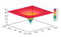
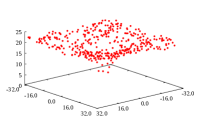
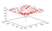
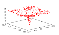
Figure 1: An overview of the space net optimization that contains the operators for region search (RS), point search (PS), space net adjustment (SNA), and population adjustment (PA).

(a)	(b)	(c)	(d)

Figure 2: A simple example that applies space net optimization to the 2-D Ackley function to explain its convergence process. (a) The landscape of the 2-D Ackley function. (b) The scattering situation of elastic points on the space net after 400 evaluations. (c) The scattering situation of elastic points on the space net after 800 evaluations. (d) The scattering situation of elastic points on the space net after 4,000 evaluations.

Until now, only a few metaheuristic algorithms focus on “extracting” the characteristics from a certain number of recent good searched solutions to guide the searches to move to particular regions (or directions). They are tabu list of tabu search (TS) Glover, (1989), personal and global best solutions of particle swarm optimization (PSO) Kennedy and Eberhart, (1995), and pheromone table of ant colony optimization (ACO) Dorigo et al., (1991, 2006). A similar idea can also be found in a more recent study Tanabe and Fukunaga, (2013) that used a “historical memory” during the convergence process to record successful control parameter settings of differential evolution (DE) to dynamically adjust the transition operations, called success-history based adaptive differential evolution (SHADE). From these studies, it can be easily seen that (1) keeping a certain number of good searched solutions (e.g., PSO Kennedy and Eberhart, (1995) and TS Glover, (1989)), (2) using a new data structure to extract the feature of subsolutions (e.g., ACO Dorigo et al., (1991)) from good searched solutions, (3) keeping a set of good parameter settings (e.g., SHADE Tanabe and Fukunaga, (2013)) are three useful ways to provide information for improving the search accuracy. Although all these metaheuristic algorithms embed mechanisms to keep the information of a certain number of searched solutions, searches are still like looking for a needle in a haystack because they all lack the knowledge of the exact landscape of the solution space or even a rough outline.

2 A Metaheuristic Algorithm with Vision of Solution Space

To explain the basic idea of the proposed algorithm, named space net optimization (SNO), a simple example is given in Fig. 2 to show the details of the major operators of SNO. The basic idea of the proposed algorithm is to use a mechanism to depict the landscape of the solution space based on the searched solutions to enhance the search performance of a metaheuristic algorithm for solving an optimization problem, just like making a map to increase the chance to find the treasure in a new place. In the initialization operator, the space net that consists of a set of elastic points $p$ will first be randomly generated in the solution space, and its role is to fit the surface of the solution space during the later convergence process. By using the space net, the elastic points can be used to divide the solution space into a set of regions $r$, each of which is associated with an expected value to describe the potential of finding a better solution in this region compared with other regions so that a set of expected values $e$ will also be generated. Two populations $s$ and $x$ will also be randomly generated in the solution space to play the roles of global search and local search, respectively. The proposed algorithm will then perform the following operators—region search (RS), point search (PS), space net adjustment (SNA), and population adjustment (PA)—repeatedly for a certain number of iterations to find the solution.

Fig. 2 also shows that the RS operator will first select a set of regions (e.g., regions $r_{4}$, $r_{5}$, and $r_{6}$) before the tournament selection kicks in to pick one of them (e.g., region $r_{6}$) to be searched later. In this example, because the objective value of the 8-th elastic point $p_{8}$ is better than those of the other three elastic points $p_{7}$, $p_{11}$, and $p_{12}$, the possible solutions will be generated around the reference point, that is, elastic point $p_{8}$. The possible solutions can be generated by either moving a solution in the population $s$ toward $p_{8}$ or moving $p_{8}$ toward a solution in the population $s$. Once a new solution $u_{i}$ is generated from $s_{i}$ to replace the current solution $s_{i}$, the SNA operator will then be used to move the top-3 elastic points of region $r_{6}$ that is close to $u_{i}$ toward this new solution. The space net will then be adjusted to fit the population $s$.

The PS operator is for the population $x$. The way a new solution $v_{i}$ is generated is similar to that of RS, but the reference point is now one of the top-$\rho$ elastic points (i.e., an elastic point with its objective value among the best $\rho$ elastic points). The PS operator will work on the space net that has already been adjusted by the RS operator to select a good elastic point (e.g., $p_{4}$) as the reference point. The possible solution can be either based on a solution in the population $x$ moving toward the selected elastic point or on the selected elastic point moving toward a solution in the population $x$. The following process is similar to but not exactly the same as the SNA after RS; that is, the SNA operator will then move the three elastic points that are closest to the new solution $v_{i}$ even closer to this new solution.

Unlike the RS and PS operators that are responsible for generating the new solutions and adjusting the space net, the PA operator is used to reduce and expand the population sizes of $s$ and $x$, as shown in the PA of Fig. 2. Because the basic idea of SNO is to use the population $s$ for global search and the population $x$ for local search, the initial population size of $s$ is set larger than the population size of $x$ to make it possible for the searches of SNO to trend to global search in the early stage of the convergence process. To make the searches of SNO gradually trend to 50% global search and 50% local search and then trend to local search in the later stage of the convergence process, PA will delete a set of solution(s) in the population $s$ and also expand the population $x$ by adding new solution(s), to adjust the ratio of the population sizes of these two populations. That is why a number of solution(s) $s_{w}$ that have the worst objective values in the population $s$ will be randomly removed first, and then new solution(s) $v_{p}$ generated around a good elastic point of the space net will be added to the population $x$.

To further show the convergence process of SNO, the 2-D Ackley function is used as the test optimization problem. Fig. 2(a) shows the landscape of the 2-D Ackley function. Figs. 2(b)–(d) show the elastic points $p$ of SNO after 400, 800, and 4,000 evaluations. Note that the number of elastic points $p$ is set equal to 400 in this example. As shown in Fig. 2(b), it can be easily seen that the elastic points are randomly distributed in the solution space during the early stage of the convergence process. As shown in Fig. 2(c), after another 400 evaluations, the distribution of the elastic points looks now a little bit like the landscape of the 2-D Ackley function. As shown in Fig. 2(d), after 4,000 evaluations, the distribution of elastic points is now much more like the landscape of the 2-D Ackley function. It is not hard to imagine that SNO now knows roughly the whole solution space, and where good solutions are likely to be found and where they are not. This also means that SNO has a full vision of the entire landscape of the solution space that the other metaheuristic algorithms do not have and thus can only base the searches on feeble vision.

3 Results

The empirical analysis is conducted on a PC with two Intel Xeon E5-2620v4 CPUs (2.10GHz, 20 MB cache, and 8 cores) and 16 GB of memory running Linux Ubuntu 18.04 x86_64, and the programs are written in C++ and compiled using g++. To evaluate the performance of the proposed algorithm (SNO), we compare it with L-SHADE Tanabe and Fukunaga, (2014), jSO Brest et al., (2017), j2020 Brest et al., (2020), NL-SHADE-RSP Stanovov et al., (2021), NL-SHADE-LBC Stanovov et al., (2022), and S-LSHADE-DP Van Cuong et al., (2022) for two well-known single objective bound constrained problem (SOP) benchmarks, CEC2021 Mohamed et al., (2020) and CEC2022 Kumar et al., (2021). The parameter settings of L-SHADE, jSO, j2020, NL-SHADE-RSP, NL-SHADE-LBC, and S-LSHADE-DP are based on Tanabe and Fukunaga, (2014); Brest et al., (2017, 2020); Stanovov et al., (2021, 2022); Van Cuong et al., (2022), respectively. The parameter settings of SNO are based on the search results of tree-structured Parzen estimator (TPE) Bergstra et al., (2011); Akiba et al., (2019). For more details of SNO, please see Section 5.2.

3.1 Comparisons of SNO and Other Search Algorithms

Fig. 3 gives the comparisons between the proposed algorithm and other state-of-the-art search algorithms for solving CEC2021 Mohamed et al., (2020) and CEC2022 Kumar et al., (2021).

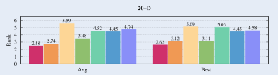
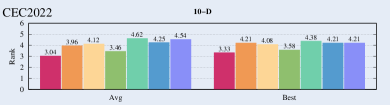
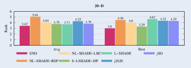
Figure 3: The average rank of each algorithm for CEC2021 and CEC2022.

They are the average rank of a search algorithm in terms of (1) the average rank of an algorithm among all algorithms for all given test functions in all trials, i.e., CEC2021 (Avg) and CEC2022 (Avg), and (2) the average rank of an algorithm among all algorithms for all given test functions in the best trial, i.e., CEC2021 (Best) and CEC2022 (Best), which are also usually used to evaluate the performance of a search algorithm for solving single objective bound constrained problems. Note that 10-D and 20-D represent 10 dimensions and 20 dimensions, respectively. The results show that (SNO) can get the best results for CEC2021 and CEC2022, which also imply that (SNO) can find the best results compared to all other search algorithms evaluated in this study for most test functions using the same maximum number of function evaluations (MaxFES).

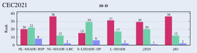
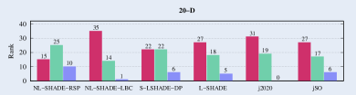
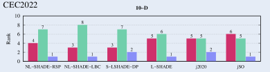
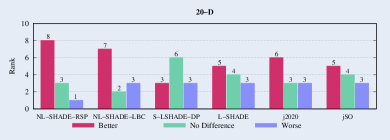
Figure 4: The comparisons between SNO and the other search algorithms for CEC2021 and CEC2022 in terms of the Wilcoxon test.

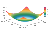
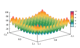
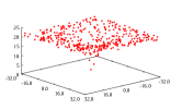
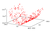
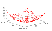
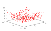
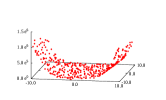
(a)	(b)	(c)	(d)	(e)
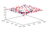
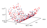
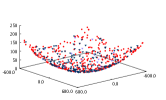
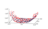
(f)	(g)	(h)	(i)	(j)
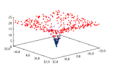
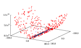
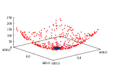
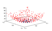
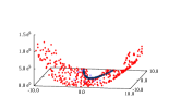
(k)	(l)	(m)	(n)	(o)
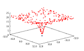
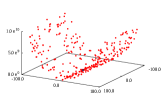
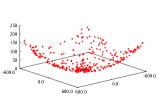
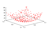
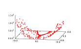
(p)	(q)	(r)	(s)	(t)

Figure 5: Simple examples that apply SNO to the Ackley, Bent Cigar, Griewank, Rastrigin, and Rosenbrock functions to explain the deformation of space net during the convergence process. (a)–(e) The scattering situation of elastic points on the space net after 400 evaluations. (f)–(j) The scattering situation of elastic points on the space net and current solutions of $s$ and $x$ after 800 evaluations. (k)–(o) The scattering situation of elastic points on the space net and current solutions of $s$ and $x$ after 4,000 evaluations. (p)–(t) The scattering situation of elastic points on the space net and current solutions of $s$ and $x$ after 20,000 evaluations. Note that the elastic points, the current solution $s$, and the current solution $x$ are marked as the red, dark blue, and light blue points in (a)–(t).

3.2 Statistical Analysis

To better understand the performance of the proposed algorithm, we also conducted a statistical analysis for the SNO and other search algorithms compared in this study. Fig. 4 shows the statistical analysis results of comparing SNO and all the other search algorithms for CEC2021 and CEC2022 in terms of the Wilcoxon test. The terms “Better,” “No Difference,” and “Worse” represent that the end result of SNO is significantly better than, not significantly better than, and worse than the compared search algorithm, respectively. The value of each search algorithm stands for the number of test functions in such a situation. For example, the results of NL-SHADE-RSP in CEC2021 show that SNO can find better results than NL-SHADE-RSP for 20 and 15 test functions with 10 dimensions and 20 dimensions. Of course, SNO cannot find better results than NL-SHADE-RSP in the other 22 and 25 test functions while there are 8 and 10 test functions the results of SNO are worse than NL-SHADE-RSP. The results also show that SNO can find better results than all the other search algorithms compared in this paper because the value of “Better” (the number of test functions that SNO outperforms the other search algorithm) is always larger than the value of “Worse” (the number of test functions that the other search algorithms outperform SNO) for all the other search algorithms in Fig. 4. Based on these comparisons and analyses, SNO can be regarded as an effective search algorithm that can provide a better way for search in general.

The convergence analysis.
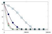
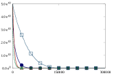
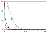
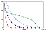
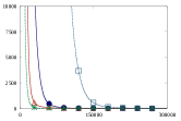
(a) Ackley	(b) Bent Cigar	(c) Griewank	(d) Rastrigin	(e) Rosenbrock
The exploration analysis
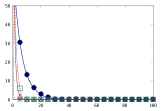
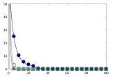
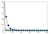
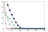
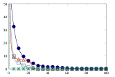
(f) Ackley	(g) Bent Cigar	(h) Griewank	(i) Rastrigin	(j) Rosenbrock
The exploitation analysis
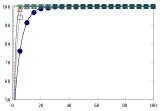
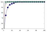
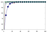
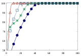
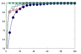
(k) Ackley	(l) Bent Cigar	(m) Griewank	(n) Rastrigin	(o) Rosenbrock
The diversity analysis
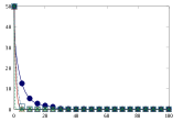
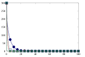
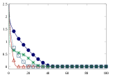
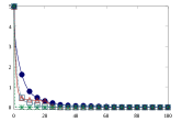
(p) Ackley	(q) Bent Cigar	(r) Griewank	(s) Rastrigin	(t) Rosenbrock

Figure 6: The analyses of convergence, exploration, exploitation, and diversity of SNO, S-LSHADE-DP, NL-SHADE-LBC, and NL-SHADE-RSP. (a)–(e) The analyses of convergence. (f)–(j) The analyses of exploration. (k)–(o) The analyses of exploitation. (p)–(t) The analyses of diversity.

3.3 The Deformation of Space Net and Change of Searches

To further understand the deformation of space net (changes of elastic points) of SNO in different situations, it is used to solve the Ackley, Bent Cigar, Griewank, Rastrigin, and Rosenbrock functions in different periods during the convergence process, as shown in Fig. 5. The landscapes of these functions are first shown on the top of the figure. In addition to the positions of the elastic points, the positions of the current solutions $s$ and $x$ are also given to show the relationship between them. All the results show that the space net will fit to the landscape gradually as the number of evaluations increases. The results also imply that the space net can provide the information of landscape to help SNO accurately determine the regions for later searches. This is why space net optimization is able to find better results than all the other metaheuristic algorithms for solving different SOPs in most cases.

3.4 Convergence Analysis

In this section, we conducted a set of convergence analyses to understand the convergence circumstance of the proposed algorithm that consist of analyses of convergence (quality), exploration (global search), exploitation (local search), and diversity (ratio of global to local search) Morales-Castañeda et al., (2020). As shown in Fig. 6 (a)–(e), the proposed algorithm is compared with other three state-of-the-art search algorithms (i.e., S-LSHADE-DP, NL-SHADE-LBC, and NL-SHADE-RSP) for five 30-$d$ basic functions—Ackley, Ben Cigar, Griewank, Rastrigin, and Rosenbrock—with 300,000 evaluations in terms of convergence. Note that the $x$-axis and $y$-axis here represent the number of evaluations and the objective value. It can be easily seen that the convergence speeds of S-LSHADE-DP and NL-SHADE-LBC are faster than SNO and NL-SHADE-RSP for most test functions, i.e., Ackley, Ben Cigar, Griewank, and Rosenbrock.

Fig. 6 (f)–(o) show that the comparisons between these four search algorithms in terms of the exploration (Fig. 6 (f)–(j)) and exploitation (Fig. 6 (k)–(o)) analyses can be regarded as the analyses of the “global search ability” and “local search ability” of each search algorithm during the convergence process, respectively. Because of the population size settings of S-LSHADE-DP Van Cuong et al., (2022), NL-SHADE-LBC Stanovov et al., (2022), and NL-SHADE-RSP Stanovov et al., (2021), the numbers of iterations these four search algorithms take are different to make them the same scale. The percentage of the convergence process is used to label the ticks of the $x$-axes of subfigures of Fig. 6 (f)–(o). Moreover, the $y$-axes of these subfigures stand for the percentage of searches focusing on exploration or exploitation. As shown in Fig. 6 (f)–(j), the percentage of exploration searches (global searches) of SNO are much higher than the other search algorithms during the period of the first 20% to 40% of the convergence process although exploration searches for all of them are decreased as the number of iterations increases. This means that SNO will prolong the global searches during the entire convergence process compared with all the other search algorithms. In Fig. 6 (k)–(o), we can first observe that the percentage of exploitation searches (local searches) of all search algorithms will increase as the number of iterations increases. The results also show that SNO will prolong the timing to increase the exploitation searches compared with the other three search algorithms. From the results of Fig. 6 (f)–(o), it can be easily seen that the time and percentage of exploration of SNO (global search) are much higher than the other search algorithms while the timing to enter the exploitation state of SNO (local search) is much late compared with the other search algorithms.

Fig. 6 (p)–(t) further provides an integrated perspective of the search abilities of different search algorithms during the convergence process that considers the exploration vs. exploitation (global search vs. local search) called diversity Morales-Castañeda et al., (2020). The $x$-axes and $y$-axes of all subfigures of Fig. 6 (p)–(t) represent the diversity and the percentage of the convergence process. The results show that the search diversities of SNO are much higher than all the other search algorithms for these five test functions. According to our observations, it is one of the most important reasons that SNO is capable of finding better results than all the other search algorithms compared in this study in most cases.

4 Discussion

In this study, we present a novel metaheuristic algorithm to solve optimization problems called space net optimization that contains a new mechanism (space net) to extract and accumulate the information of all searched solutions to depict the landscape of the solution space on the fly during the convergence process. Different from most metaheuristic algorithms that use only a few searched solutions to guide the searches, the information of the solution space constructed by space net will be used to enhance the search accuracy of SNO. Based on the design of the space net, we then design the ways to generate new candidate solutions of SNO to refer to not only the current solutions but also the elastic points of the space net. In such a design, current solutions can be regarded as the current positions we are and elastic points can be regarded as the map of the space we have. That is why the metaheuristic algorithm will now have the vision on the solution space as we pointed out in the very beginning of this paper. The simulation results show that SNO outperform all the other state-of-the-art search algorithms for complex SOPs compared in this study. One of our future works will be on applying the proposed algorithm to the other kind of optimization problem, such as combinatorial optimization problem. Another future work is to develop a more effective way to construct the space net to depict the solution space to enhance the search ability of SNO.

5 Methods

5.1 Problem Definition

The single objective bound constrained problem (SOP) is a well-known global optimization problem, which can be found in many real-world scientific and engineering applications in our daily life. An SOP can be formulated as:

Definition 1.

Given a function and a set of constraints, this problem aims to find the optimum objective value, subject to the constraints, out of all the feasible solutions of the function.

$$\min\limits_{s\in\mathbf{R}^{d}}f(s),\mathop{\rm subject~{}to}\ \forall f_{j}(s)\mathop{\rm\odot}b_{j},j=1,2,\dots,m,$$

where

• $s=(s_{1},s_{2},\dots,s_{d})$ is a feasible solution, $d$ is the number of dimensions, and $s_{i}$ is in the range $[L_{i},U_{i}]$, where $L_{i}$ and $U_{i}$ are the lower and upper bounds of the $i$-th dimension;

• $f(s):\mathbf{R}^{d}\to\mathbf{R}$ is the objective function to be optimized,

• $f_{j}(s):\mathbf{R}^{d}\to\mathbf{R}\mathop{\rm\odot}b_{j}$ is the $j$-th constraint where $\mathop{\rm\odot}$ is either $<$, $>$, $=$, $\leq$, or $\geq$, $m$ is the number of constraints, and

• $\mathbf{R}^{d}$ and $\mathbf{R}$ are the domain and codomain.

As for a search algorithm, the goal of this problem is to find out a “good” solution that has the best objective value from the whole solution space (i.e., the set of all feasible solutions). With Definition 1 at hand, we can now use it to describe an optimization problems that we would like to test. The Ackley function Ackley, (1987); Bäck, (1996) can be used as an example to use this definition to describe SOP.

Definition 2 (The Ackley optimization problem).

$$\min\limits_{s\in\mathbf{R}^{n}}f(s)=-20\exp\left(-0.2\sqrt{\frac{1}{n}\sum_{i=1}^{n}s_{i}^{2}}\right)\\ \hfill{}-\exp\left(\frac{1}{n}\sum_{i=1}^{n}\cos(2\pi s_{i})\right)+20+e,\\ \mathop{\rm subject~{}to}\ -30\leq s_{i}\leq 30,i=\mathop{\rm 1,2},\dots,d.$$

It can be easily seen from Definition 2 that a feasible solution of the Ackley function is within the hypercube $s_{i}\in[\,-30,30\,]$, $\forall i=1,2,\dots,d$. The global optimum (minimum) of the Ackley function is $f(s_{b})=0$ located at $s_{b}=(0,0,\dots,0)$. As shown in Fig. 2(a), an Ackley function (i.e., $d=2$) has many local optima that make it difficult for a search algorithm to find the global optimum from the starting point(s) randomly chosen from the entire solution space. That is why it was widely used as the touchstone to understand the performance of a search algorithm.

The experimental settings of the maximum number of function evaluations (MaxFES) for the test functions (CEC2021 and CEC2022) are with different number of dimensions. In this study, MaxFES is set equal to 200,000 for the number of dimensions $d=10$ and equal to 10,00,000 for the number of dimensions $d=20$. Note that a search algorithm will be terminated when MaxFES is reached or when the error value is smaller than $10^{\textendash 8}$ for each test in the search range $[\,-100,100\,]^{d}$.

5.2 Details of the Proposed Algorithm

To simplify the discussion of the proposed algorithm, the following notation will be used throughout this section.

• a set of explorers, i.e., $s=\{s_{1},s_{2},\dots,s_{n_{s}}\}$, where $s_{i}$ is the $i$-th explorer, and $n_{s}$ is the population size of $s$. Moreover, $s_{i,j}$ is the $j$-th dimension of the $i$-th explorer, and $u$ is a set of temporary explorers generated from $s$.

• a set of miners, i.e., $x=\{x_{1},x_{2},\dots,x_{n_{x}}\}$, where $x_{i}$ is the $i$-th miner, and $n_{x}$ is the population size of $x$. Moreover, $x_{i,j}$ is the $j$-th dimension of the $i$-th miner, and $v$ is a set of temporary miners generated from $v$.

• the space net, i.e., $p=\{p_{1},p_{2},\dots,p_{n_{p}}\}$, where $p_{i}$ is the $i$-th elastic point of the space net, and $n_{p}$ is the population size of $p$ (i.e., the number of elastic points in the space net). Moreover, $p_{i,j}$ denotes the $j$-th dimension of the $i$-th elastic point, $q$ a set of elastic points generated from $p$, and $n_{a}$ how many elastic points will be attracted and moved toward to a new candidate solution of an explorer or a miner.

• a set of regions used to allocate the elastic points in the space net, i.e., $r=\{r_{1},r_{2},\dots,r_{h}\}$, where $r_{i}$ is the $i$-th region; $h$ the number of regions, which is set equal to $h=(\sqrt{n_{p}}-1)^{2}$; $r_{i,k}$ the $k$-th elastic point at the $i$-the region; and $r_{i,b}$ the best elastic point at the $i$-th region.

• a set of expected value $e=\{e_{1},e_{2},\dots,e_{h}\}$, each of which consists of the visited ratio, improvement value, and best value of the $i$-th region, respectively.

• sets of control parameter, i.e., $\alpha=\{\alpha_{1},\alpha_{2},\dots,\alpha_{h}\}$ and $\beta=\{\beta_{1},\beta_{2},\dots,\beta_{h}\}$, where $\alpha_{i}$ and $\beta_{i}$ represent the crossover rate and scaling factor associated with the $i$-th region.

• two control factors to control the search of RS and PS.

• the ratio of the number of function evaluations performed so far FES to the predefined maximum number of function evaluations $\text{FES}_{\max}$, i.e., $\delta=\frac{\text{FES}}{\text{FES}_{\max}}$.

• an adjustment function to get the adaptive value of the given parameter $v$ that will increase or decrease from its initial value $a$ to the end value $b$ via $a+\delta(b-a)$, i.e., $\lambda(\delta)_{1}^{2}$ stands for the adaptive value of this function will be computed as $1+\delta(2-1)$ where $a=1$ and $b=2$.

• a random number uniformly distributed in the range $[0,1]$.

• $t$ is the current iteration number and $t_{\max}$ is the maximum number of iterations.

As we mentioned before, the parameter settings of SNO are based on the search results of TPE Bergstra et al., (2011); Akiba et al., (2019). The detailed parameter settings of SNO are as follows: $n_{\psi}^{\text{init}}$ represent the initial value of $n_{\psi}$ where ${\psi}\in\{s,x,\alpha,\beta\}$; and $n_{x}^{\text{end}}$ the end value (maximum value) of $n_{x}$. Based on the search results of TPE, we have the following settings: ${n_{s}}^{\text{init}}=190$, ${n_{x}}^{\text{init}}=0.1\times{n_{s}}^{\text{init}}$, ${n_{x}}^{\text{end}}=0.2\times{n_{s}}^{\text{init}}$, and ${n_{p}}=9^{2}$. We also have the following settings: ${\rho}_{\max}=0.7$, ${\alpha}^{\text{init}}=0.5$, and ${\beta}^{\text{init}}=0.1$, $c_{s}=2.0$, and $c_{x}=2.5$ for SNO.

Algorithm 1 is an outline of the proposed algorithm. As shown in Algorithm 1, the inputs are the objective function and the parameter settings of the proposed algorithm while the output is the best found solution $s_{b}$ (i.e., best so far solution).

Algorithm 1 Space Net Optimization

1:The objective function $f()$ and parameter settings of SNO.

2:Best found solution $s_{b}$.

3:Initialization()

4:while $t<t_{\max}$ do

5:    $e$ = ExpectedValue($r$)

6:    $u$ = RegionSearch($s$, $p$, $e$, $r$)

7:    $q$ = SpaceNetAdjustment($u$, $p$, $e$, $r$)

8:    $v$ = PointSearch($x$, $q$, $e$, $r$)

9:    $q$ = SpaceNetAdjustment($v$, $p$, $e$, $r$)

10:    $u$, $v$ = PopulationAdjustment($u$, $v$, $q$, $e$, $r$)

11:    $s_{b}$ = UpdateBestSoFar($s$, $x$, $u$, $v$)

12:    $s$ = $u$, $x$ = $v$, $p$ = $q$

13:    $t=t+1$

14:end while

15:return The best found solution $s_{b}$

The initialization operator will be invoked first to initialize SNO that includes the populations $s$ and $x$, elastic points on the space net $p$, regions $r$, expected values $e$, best found solution $s_{b}$, and two control parameter sets $\alpha$ and $\beta$ based on the inputs and random procedure. SNO will then perform the operators ExpectedValue(), RegionSearch(), PointSearch(), SpaceNetAdjustment(), PopulationAdjustment(), and BestSoFar(), iteratively. Among them, the BestSoFar() operator is the most simple operator compared with the other operators, which will be used to update the best found solution, that is, the best so far solution, during the convergence process. The other operators of SNO will be described in detail below.

5.2.1 Expected Value

The expected value of SNO is inspired by Tsai, (2016) where it stated that the objective/fitness value of “a solution” can be replaced by the expected value of “a region” of the solution space for a novel metaheuristic algorithm (search economics; SE) to avoid the searches trending to particular solutions. The expected value of a region in SE is composed of (1) the ratio of the number of time the region has been searched to the number of times the region region has not been searched, (2) the average objective value of new candidate solutions generated in the region, and (3) the objective value of the best-so-far solution in the region. Different from the expected value of most SEs, the expected value of SNO will use the improvement value of elastic points belonging to a region to replace the average objective value of the new candidate solutions generated in the $j$-th region. The expected value of a region, say, the $i$-th region $e_{i}$, in SNO is thus defined as

$$\begin{split}e_{i}=&\mathcal{N}\left(\frac{I^{b}_{i}}{I^{a}_{i}}\right)+\mathcal{N}\left(\sum_{j=1}^{4}\left(f(r_{i,j}^{t-1})-f(r_{i,j}^{t})\right)\right)\\ &\quad{}+\lambda(\delta)_{2}^{1}\cdot\left(1.0-\mathcal{N}(f(r_{i,b}^{t}))\right),\end{split}$$ (1)

where the first term of Eq. (1) represents the impact of the visited ratio, where $I^{a}_{i}$ and $I^{b}_{i}$ represent the number of times the region has been visited and has not been visited. The second term represents the impact of the sum of the improvement value of the elastic points that belong to the $i$-th region at the $t$-th iteration. The third term represents the impact of the objective value of the best elastic point belonging to the $i$-th region at the $t$-th iteration. Besides, $\mathcal{N}()$ and $f()$ represent the normalization and objective functions, respectively.

5.2.2 Region Search

The region search operator plays the role of generating new candidate solutions $u$ from the population $s$ for “exploration.” In this operator, a number of regions (i.e., $\lambda(\delta)_{0.1}^{1.0}\times h$) will first be selected from all regions $r$ based on their expected values in $e$. The number of selected top regions $\lambda(\delta)_{0.1}^{1.0}\times h$ will be decreased gradually from $h$ at the very beginning down to $0.1\times h$ during the convergence process. These selected regions will then be used in the roulette wheel selection to determine a region $r^{\text{sel}}_{i}$ based on the expected values in $e$. A reference point $p_{i}^{\text{sel}}$ will then be picked from the selected region $r^{\text{sel}}_{i}$ to generate the new candidate solution of population $s$. The reference point generation is defined as

$$p_{i}^{\text{sel}}=\begin{cases}\text{Tourn}(r^{\text{sel}}_{i}),&\text{if}~{}\phi<\lambda(\delta)_{0.1}^{1.0},\\ r_{i,b}^{\text{sel}},&\text{otherwise},\end{cases}$$ (2)

where $\text{Tourn}(r^{\text{sel}}_{i})$ represents the tournament selection for the region $r^{\text{sel}}_{i}$ that will select an elastic point while $r_{i,b}^{\text{sel}}$ represents the best elastic point in the selected region $r^{\text{sel}}_{i}$.

Now, the region search operator will use the reference point to generate a new candidate solution $u_{i}$ of population $s$. A random number $j_{\text{rand}}$ in the range $[1,d\,]$ will be first generated for $u_{i}$; another random number $\phi_{c}$ in the range $[0,1]$ will then be generated for $u_{i,j}$ to determine whether to generate a new candidate value or use the value in $s_{i,j}$ as the value of the $j$-th dimension of the new candidate solution $u_{i,j}$, which is similar to the crossover operator of DE Storn and Price, (1997). In case $\phi_{c}\geq\alpha_{i}$ and $j\neq j_{\text{rand}}$,

$$u_{i,j}=s_{i,j},$$ (3)

where $\alpha_{i}$ is a crossover value associated with $r^{\text{sel}}_{i}$. In case $\phi_{c}<\alpha_{i}$ or $j=j_{\text{rand}}$, the $j$-th dimension of $u_{i}$ will be calculated as follows:

$$u_{i,j}=\begin{cases}p_{i,j}^{\text{sel}}+\beta_{i}\times\left(s_{r_{1},j}-s_{r_{2},j}\right),&\text{if}~{}\phi<{\delta^{c_{s}}},\\ s_{i,j}+\beta_{i}\times\left(p_{i,j}^{\text{sel}}-s_{r_{1},j}\right),&\text{otherwise},\end{cases}$$ (4)

where $\beta_{i}$ is the scaling factor associated with $r^{\text{sel}}_{i}$. At the end of the region search, if $f(u_{i})$ is better than $f(s_{i})$, it will be used to replace the $s_{i}$ at next iteration.

5.2.3 Point Search

The point search operator is used to generate the new candidate solutions $v$ from population $s$ that is similar to the region search, but for “exploitation.” Like the Eqs. (3) and (4) of region search, it will first generate a random number $\phi_{c}$ for $v_{i}$ and a random number $j_{\text{rand}}$ for $v_{i,j}$. If $\phi_{c}\geq\alpha_{i}$ and $j\neq j_{\text{rand}}$, $v_{i,j}$ will be set equal to $x_{i,j}$; otherwise, the value of the $j$-th dimension of $x_{i}$ can be calculated as follows:

$$v_{\phi_{x},j}=\begin{cases}p_{\phi_{x},j}^{\text{top-}\rho}+\beta_{i}\times\left(x_{r_{1},j}-x_{r_{2},j}\right),&\text{if}~{}\phi<{\delta^{c_{x}}},\\ x_{\phi_{x},j}+\beta_{i}\times\left(x_{r_{1},j}-x_{r_{2},j}\right),&\text{otherwise},\end{cases}$$ (5)

where $\phi_{x}$ is a random number in the range $[1,n_{x}]$. However, there are some differences between region search and point search operators. The first difference is that the $i$-th update of region search is for the $i$-th solution $s_{i}$ at each iteration, but it will be a random one $x_{\phi_{x}}$ for point search. The second difference is that the $i$-th new candidate solution $p^{\text{sel}}_{i}$ in region search is to select one elastic point by roulette wheel then tournament selections from the elastic points belonging to the specific region, but the $i$-th new candidate solution $p_{\phi_{x}}^{\text{top}-\rho}$ in point search is to randomly select one elastic point from top-$\rho$ elastic points of all elastic points in the space net. The value of $\rho$ is set equal to $\lambda(\phi)_{0.1}^{\rho_{\max}}$ where $\rho_{\max}$ is the maximum value of $\rho$. Like the region search, if $f(v_{\phi_{x}})$ is better than $f(x_{\phi_{x}})$, it will be used to replace $x_{\phi_{x}}$ at next iteration.

5.2.4 Space Net Adjustment

The role of space net in SNO is to depict the landscape based on the searched solutions of $s$ and $x$.

This operator will first update how many elastic points will be attracted by a newly candidate solution $u_{i}$ from region search (or new candidate solution $v_{i}$ generated from point search) that is defined as follows:

$$n_{a}=\lceil n_{a,\max}\times\delta\rceil,$$ (6)

where $n_{a,\max}$ represents the predefined maximum number of elastic points that will be attracted by a newly candidate solution. In this study, ${n_{a,\max}}$ is set equal to 5. To update the location of elastic points, in addition to the solutions at $t$ iteration (i.e., $s$ and $x$), solutions at $t+1$ iteration are also used to “replace” the elastic points of space net. Two additional ways that can also be used to generate the reference point to move the elastic points are defined as follows:

$$p_{i}^{a}=\nu+\beta_{i}\cdot(\nu_{r_{1}}-\nu_{r_{2}}),$$ (7)

$$p_{i}^{b}=p_{i}+\beta_{i}\cdot(\nu-p_{i})+\beta_{i}\cdot(\nu_{r_{1}}-\nu_{r_{2}}),$$ (8)

where $\nu\in\{u_{\phi_{u}},v_{\phi_{v}}\}$ and $\nu_{r_{1}},\nu_{r_{2}}\in\{s_{\phi_{s}},x_{\phi_{x}}\}$, with $\phi_{u},\phi_{v},\phi_{s},\phi_{x}$ representing a random number in the ranges $[1,n_{u}]$, $[1,n_{v}]$, $[1,n_{s}]$, and $[1,n_{x}]$, respectively. Similar to the new candidate solution generation of region search (e.g., Eqs. (3) and (4)), the $j$-th dimension of new candidate solution $q^{a}_{i}$ and $q^{b}_{i}$ will also be checked to see if $\phi_{c}<\alpha_{i}$ or $j$ is equal to a random number $j_{\text{rand}}$. If yes, $q^{a}_{i,j}$ will set equal to $p^{a}_{i,j}$; otherwise, $q^{a}_{i,j}$ will be set equal to $p_{i,j}$. Also, the same checks and updates will also be used for $q^{b}_{i,j}$. After that, the new candidate solution $q_{i}$ will be generated as follows:

$$q_{i}=\begin{cases}\nu,&\text{if}~{}i=1,\\ \text{Dist}_{\min}(q^{a}_{i},q^{b}_{i},\nu),&\text{if}~{}i\neq 1~{}\text{and}~{}\phi<\delta,\\ \text{Dist}_{\min}(q^{a}_{i},q^{b}_{i},p_{i}),&\text{otherwise},\end{cases}$$ (9)

where $\text{Dist}_{\min}(g_{1},g_{2},g_{3})$ is a function to find out the most closest solution (i.e., $g_{1}$ or $g_{2}$) of solution $g_{3}$. Last, if $f(q_{i})$ is better than $f(p_{i})$, it will be used to replace $p_{i}$ at next iteration.

5.2.5 Population Adjustment

One major task of this operator is to adjust the size of populations $s$ and $x$, as follows:

$$n=\lambda(\delta^{(1-\sqrt{\delta})})_{n_{\text{init}}}^{n_{\text{end}}},$$ (10)

where $n$ can be either the value of $n_{s}$ or $n_{x}$. By using this equation to adjust the population size of $s$, $n_{s}$ will be set equal to $n$, $n_{\text{init}}$ a predefined population size of $s$ at the very beginning, and $n_{\text{end}}$ a predefined population size of $s$ at the end during the convergence process of SNO. Of course, this equation will also be used to adjust the population size of $x$ during the convergence process. The main difference between $s$ and $x$ for the population resize using Eq. (10) is that the population size of $s$ will be reduced gradually while the population size of $x$ will be increased gradually. For this reason, the values of $n_{\text{init}}$ is larger than $n_{\text{end}}$ for $s$ while $n_{\text{init}}$ is smaller than $n_{\text{end}}$ for $x$.

In addition to the population size adjustment, this operator will also generate the new candidate solution $v_{p}$ that is the third way to generate a new candidate solution of SNO. Note that the other two are by using the RS and PS operators. The $j$-th dimension of $v_{p}$ will be generated as follows:

$$v_{p,j}=\begin{cases}\delta^{2}\cdot p_{\phi_{i},j}^{\text{top-}\rho}+(1-\delta^{2})\cdot\phi^{U_{i}}_{L_{i}},&\text{if}~{}\phi<0.5,\\ p_{\phi_{i},j}^{\text{top-}\rho},&\text{otherwise},\end{cases}$$ (11)

where $p_{\phi_{i}}^{\text{top-}\rho}$ is a randomly selected elastic point from the top-$\rho$ elastic points in terms of the objective value, which is the same as Eq. (5), and $\phi^{U_{i}}_{L_{i}}$ is a random number uniformly distributed in the range $[L_{i},U_{i}]$.

5.2.6 Summary

A detailed discussion of the proposed algorithm was given in Section 5.2 that is used for solving SOPs in Section 3. We will now turn our discussion to the roles and relationships of three populations and how to generate new candidate solutions by three different operators, to explain the distinguishing features of SNO. One of the distinguishing features of SNO is that it will generate three populations for the search. Among them, explorers $s$ and miners $x$ can be regarded as the searched solutions at each iteration while elastic points $p$ that belong to space net can be regarded as the accumulated information of all searched solutions from the very beginning until the current iteration. The population size of $s$, $x$, and $p$ are $n_{s}$, $n_{x}$, and $n_{p}$, respectively, and $n_{a}$ is used to determine how many elastic points will be affected by new solutions $u$ and $v$. The roles of explorers and miners are for the global and local search during the convergence process, which imply that explorers will search for larger scope than miners in the solution space. That is why the population size of $s$ will be decreased while the population size of $x$ will be increased during the convergence process. The role of $p$ is to keep and provide information of the landscape of the solution space, which will be used in the calculation of the expected value so that SNO will make accurate searches. The number of elastic points in $p$ will not be changed during the convergence process. Another distinguishing feature of SNO is that it will generate new candidate solutions by region search (i.e., a certain number of new explorers $u$), point search (i.e., a certain number of new miners $v$), and population adjustment (i.e., a certain number of new miners $v_{p}$). In addition to point search, SNO uses population adjustment to generate another new miner $v_{p}$ because (1) it needs to increase the number of miners when SNO determines to decrease the population size of $s$ and increase the population size of $x$, and (2) it uses another strategy to generate the new candidate solution to increase the search diversity.

References

- Ackley, (1987) Ackley, D. H. (1987). A Connectionist Machine for Genetic Hillclimbing. Kluwer Academic Publishers, Norwell, MA.
- Akiba et al., (2019) Akiba, T., Sano, S., Yanase, T., Ohta, T., and Koyama, M. (2019). Optuna: A next-generation hyperparameter optimization framework. In Proceedings of the ACM SIGKDD International Conference on Knowledge Discovery & Data Mining, pages 2623–2631.
- Bäck, (1996) Bäck, T. (1996). Evolutionary Algorithms in Theory and Practice: Evolution Strategies, Evolutionary Programming, Genetic Algorithms. Oxford University Press, Inc., New York, NY.
- Bergstra et al., (2011) Bergstra, J., Bardenet, R., Bengio, Y., and Kégl, B. (2011). Algorithms for hyper-parameter optimization. In Proceedings of Advances in Neural Information Processing Systems, pages 2546–2554.
- Blum and Roli, (2003) Blum, C. and Roli, A. (2003). Metaheuristics in combinatorial optimization: Overview and conceptual comparison. ACM Computing Surveys, 35(3):268–308.
- Brest et al., (2020) Brest, J., Maučec, M. S., and Bošković, B. (2020). Differential evolution algorithm for single objective bound-constrained optimization: Algorithm j2020. In Proceedings of the IEEE Congress on Evolutionary Computation, pages 1–8.
- Brest et al., (2017) Brest, J., Maučec, M. S., and Bošković, B. (2017). Single objective real-parameter optimization: Algorithm jSO. In Proceedings of the IEEE Congress on Evolutionary Computation, pages 1311–1318.
- Dorigo et al., (2006) Dorigo, M., Birattari, M., and Stutzle, T. (2006). Ant colony optimization. IEEE Computational Intelligence Magazine, 1(4):28–39.
- Dorigo et al., (1991) Dorigo, M., Maniezzo, V., and Colorni, A. (1991). Ant System: An autocatalytic optimizing process. Technical report, Dipartimento di Elettronica, Politecnico di Milano, Italy. Technical Report 91-016, Available at https://citeseerx.ist.psu.edu/viewdoc/download?rep=rep1&type=pdf&doi=10.1.1.51.4214, Accessed 22.08.01.
- Glover, (1989) Glover, F. (1989). Tabu search—part I. ORSA Journal on Computing, 1(3):190–206.
- Glover and Kochenberger, (2003) Glover, F. and Kochenberger, G. A., editors (2003). Handbook of Metaheuristics. Kluwer Academic Publishers, Boston, MA.
- Huang et al., (2020) Huang, Y., Li, W., Tian, F., and Meng, X. (2020). A fitness landscape ruggedness multiobjective differential evolution algorithm with a reinforcement learning strategy. Applied Soft Computing, 96:106693.
- Kennedy and Eberhart, (1995) Kennedy, J. and Eberhart, R. C. (1995). Particle swarm optimization. In Proceedings of the IEEE International Conference on Neural Networks, pages 1942–1948.
- Kumar et al., (2021) Kumar, A., Price, K. V., Mohamed, A. W., Hadi, A. A., and Suganthan, P. N. (2021). Problem definitions and evaluation criteria for the 2022 special session and competition on single objective bound constrained numerical optimization. Technical report, Nanyang Technological University, Singapore.
- Li et al., (2023) Li, B., Wei, Z., Wu, J., Yu, S., Zhang, T., Zhu, C., Zheng, D., Guo, W., Zhao, C., and Zhang, J. (2023). Machine learning-enabled globally guaranteed evolutionary computation. Nature Machine Intelligence, 5:457–467.
- (16) Liu, X., Sun, J., Zhang, Q., Wang, Z., and Xu, Z. (2023, In Press). Learning to learn evolutionary algorithm: A learnable differential evolution. IEEE Transactions on Emerging Topics in Computational Intelligence, pages 1–16.
- Liu et al., (2023) Liu, Y., Sun, Y., Xue, B., Zhang, M., Yen, G. G., and Tan, K. C. (2023). A survey on evolutionary neural architecture search. IEEE Transactions on Neural Networks and Learning Systems, 34(2):550–570.
- Mohamed et al., (2020) Mohamed, A. W., Hadi, A. A., Mohamed, A. K., Agrawal, P., Kumar, A., and Suganthan, P. N. (2020). Problem definitions and evaluation criteria for the CEC 2021 special session and competition on single objective bound constrained numerical optimization. Technical report, Nanyang Technological University, Singapore.
- Morales-Castañeda et al., (2020) Morales-Castañeda, B., Zaldívar, D., Cuevas, E., Fausto, F., and Rodríguez, A. (2020). A better balance in metaheuristic algorithms: Does it exist? Swarm and Evolutionary Computation, 54:100671.
- Stanovov et al., (2021) Stanovov, V., Akhmedova, S., and Semenkin, E. (2021). NL-SHADE-RSP algorithm with adaptive archive and selective pressure for CEC 2021 numerical optimization. In Proceedings of the IEEE Congress on Evolutionary Computation, pages 809–816.
- Stanovov et al., (2022) Stanovov, V., Akhmedova, S., and Semenkin, E. (2022). NL-SHADE-LBC algorithm with linear parameter adaptation bias change for CEC 2022 numerical optimization. In Proceedings of the IEEE Congress on Evolutionary Computation, pages 01–08.
- Storn and Price, (1997) Storn, R. and Price, K. (1997). Differential evolution – A simple and efficient heuristic for global optimization over continuous spaces. Journal of Global Optimization, 11(4):341–359.
- Tanabe and Fukunaga, (2013) Tanabe, R. and Fukunaga, A. (2013). Success-history based parameter adaptation for differential evolution. In Proceedings of the IEEE Congress on Evolutionary Computation, pages 71–78.
- Tanabe and Fukunaga, (2014) Tanabe, R. and Fukunaga, A. S. (2014). Improving the search performance of SHADE using linear population size reduction. In Proceedings of the IEEE Congress on Evolutionary Computation, pages 1658–1665.
- Tsai, (2016) Tsai, C. W. (2016). An effective WSN deployment algorithm via search economics. Computer Networks, 101:178–191.
- (26) Tsai, C.-W. and Chiang, M.-C. (2023 (To Appear)). Handbook of Metaheuristic Algorithms: From Fundamental Theories to Advanced Applications. Elsevier.
- Van Cuong et al., (2022) Van Cuong, L., Bao, N. N., Phuong, N. K., and Binh, H. T. T. (2022). Dynamic perturbation for population diversity management in differential evolution. In Proceedings of the Genetic and Evolutionary Computation Conference Companion, pages 391–394.
- Yang and Shami, (2020) Yang, L. and Shami, A. (2020). On hyperparameter optimization of machine learning algorithms: Theory and practice. Neurocomputing, 415:295–316.