Explainability in Simplicial Map Neural Networks

Abstract

Simplicial map neural networks (SMNNs) are topology-based neural networks with interesting properties such as universal approximation capability and robustness to adversarial examples under appropriate conditions. However, SMNNs present some bottlenecks for their possible application in high dimensions. First, no SMNN training process has been defined so far. Second, SMNNs require the construction of a convex polytope surrounding the input dataset. In this paper, we propose a SMNN training procedure based on a support subset of the given dataset and a method based on projection to a hypersphere as a replacement for the convex polytope construction. In addition, the explainability capacity of SMNNs is also introduced for the first time in this paper.

1 Introduction

In the last years, Artificial Intelligence (AI) methods in general, and Machine Learning methods in particular, have reached a success level on real-life problems unexpectedly only a few years ago. Many different areas have contributed to this development. Among them, we can cite research on new theoretical algorithms, the increasing computational power of the hardware of the last generation, and the quick access to a huge amount of data. Such a combination of factors leads to the development of more and more complex self-regulated AI methods.

Many of the AI models currently used are based on backpropagation algorithms, which train and regulate themselves to achieve a goal, such as classification, recommendation, or prediction. These self-regulating models achieve some kind of knowledge as they successfully evaluate test data independent of the data used to train them. In general, such knowledge is not understandable by humans in its current representation, since it is implicit in a large number of parameters and their relationships, which are immeasurable to the human mind. Due to its lack of explainability, the application of AI models generates rejection among citizens, and many governments are imposing limits on their use. At the same time, experts in social sciences, medicine, and many other areas do not usually trust the decisions made by AI models since they cannot follow the argument that leads to the final decision.

To fill the gap between the recent development of AI models and their social use, many researchers have focused on the development of Explainable Artificial Intelligence (XAI), which consists of a set of techniques to provide clear, understandable, transparent, intelligible, trustworthy, and interpretable explanations of the decisions, predictions, and reasoning processes made by the IA models, rather than just presenting their output, especially in domains where AI decisions can have significant consequences on human life.

Some of the recent applications of XAI in real-life problems include healthcare [4, 11], laws [2], radiology [8], medical image [9], or education [10] In general, these approaches to XAI follow the main guideline of representing implicit knowledge in the AI model in a human-readable fashion. For example, some methods try to provide an explanation through data visualization [1] (by plotting the importance of the feature, the local representation of a specific observation, etc.). Other methods try to provide an explanation by using other AI models that are more human-readable (such as decision trees or linear regression [17]). A global taxonomy of interpretable AI with the aim of unifying terminology to achieve clarity and efficiency in the definition of regulations for the development of ethical and reliable AI can be found in [7]. A nice introduction and general vision can be found in [12]. Another clarifying paper with definitions, concepts, and applications of XAI is [13].

In this paper, we provide a contribution to XAI from a topological perspective. In this way, we provide a trainable version of the so-called Simplicial Map Neural Networks (SMNN) that were introduced in [14] as a constructive approach to the problem of approximating a continuous function on a compact set in a triangulated space. SMNNs were built as a two-hidden-layer feedforward network where the set of weights was precomputed. The architecture of the network and the computation of the set of weights were based on a combinatorial topology tool called simplicial maps and the triangulation of the space. From an XAI point of view, SMNN is an explainable model, since all the decision steps in order to compute the output of the network were understandable and transparent, and therefore trustworthy.

The paper extends the concept of SMNNs that is based on considering the $n$-dimensional space of the input labeled dataset (where $n$ is the number of features) as a triangulable metric space by building a combinatorial structure (a simplicial complex) on top of the dataset and constructing a neural network based on a simplicial map defined between such simplicial complex and a simplex representing the label space (see details below). One of the drawbacks of this approach is the calculation of the exact weights of the neural network, being the whole computation extremely expensive. In this paper, we propose a method to approximate such weights based on optimization methods with competitive results. A second drawback of the definition of SMNNs is the set of points chosen as the vertices of the triangulation. In this paper, we also provide a study on these points (the so-called support points) and propose alternatives to make SMNNs more efficient.

The paper is organized as follows. First, some concepts of computational topology and the definition of SMNNs are recalled in Section 2. Next, Section 3 develops several technical details needed for the SMNN training process, which will be introduced in Section 5. Section 6 is devoted to the explainability of the model. Finally, the paper ends with some experiments and final conclusions.

2 Background

In this section, we assume that the reader is familiar with the basic concepts of computational topology. For a comprehensive presentation, we refer to [5].

2.1 Simplicial complexes

Consider a finite set of points $V=\{v^{1},\dots,v^{\beta}\}\subset\mathbb{R}^{n}$. whose elements will be called vertices. A subset

$$\sigma=\langle v^{i_{0}},v^{i_{1}},\dots,v^{i_{d}}\rangle$$

of $V$ with $d+1$ vertices (in general position) is called a $d$-simplex. The convex hull of the vertices of $\sigma$ will be denoted by $|\sigma|$ and corresponds to the set:

$$\Big{\{}x\in\mathbb{R}^{n}:\,x=\sum_{\scriptscriptstyle j\in[\![0,d]\!]}b_{j}(x)v^{i_{j}}\Big{\}}$$

where $[\![0,d]\!]=\{0,1,\dots,d\}$ and

$$b(x)=(b_{0}(x),b_{1}(x),\dots,b_{d}(x))$$

are called the barycentric coordinates of $x$ with respect to $\sigma$, and satisfy that:

$$\mbox{$\sum_{\scriptscriptstyle j\in[\![0,d]\!]}b_{j}(x)=1\;\mbox{ and }\;b_{j}(x)\geq 0\;\forall j\in[\![0,d]\!]$}\,.$$

For example, let us consider the 1-simplex $\epsilon=\langle v^{i_{0}},v^{i_{1}}\rangle$ which is composed by two vertices of $V$. Then $|\epsilon|$ is the set of points in $\mathbb{R}^{n}$ corresponding to the edge with endpoints $v^{i_{0}}$ and $v^{i_{1}}$, and if, for example, $b(x)=(\frac{1}{2},\frac{1}{2})$ then $x$ is the midpoint of $|\epsilon|$.

A simplicial complex $K$ with vertex set $V$ consists of a finite collection of simplices satisfying that if $\sigma\in K$ then either $\sigma=\langle v\rangle$ for some $v\in V$ or any face (that is, nonempty subset) of $\sigma$ is a simplex of $K$. In addition, if $\sigma,\mu\in K$ then, either $|\sigma|\cap|\mu|=\emptyset$ or $|\sigma|\cap|\mu|=|\gamma|$ for some $\gamma\in K$. The set $\bigcup_{\sigma\in K}|\sigma|$ will be denoted by $|K|$. A maximal simplex of $K$ is a simplex that is not the face of any other simplex of $K$. If the maximal simplices of $K$ are all $d$-simplices then $K$ is called a pure $d$-simplicial complex. See the example shown in Figure 1.

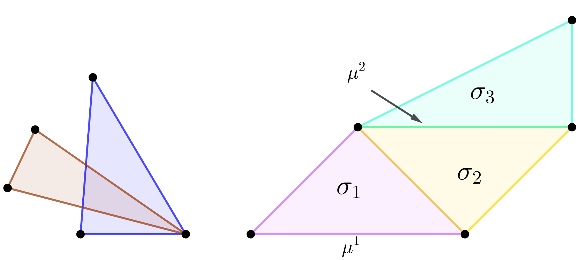
Figure 1: On the left, two triangles that do not intersect in a common face (an edge or a vertex) are shown. On the right, the geometric representation $|K|$ of a pure 2-simplicial complex $K$ composed of three maximal $2$-simplices (the triangles $\sigma^{1}$, $\sigma^{2}$ and $\sigma^{3}$). The edge $\mu^{2}$ is a common face of $\sigma^{2}$ and $\sigma^{3}$. The edge $\mu^{1}$ is a face of $\sigma^{1}$.

The barycentric coordinates of $x$ with respect to the simplicial complex $|K|$ are defined as the barycentric coordinates of $x$ with respect to $\sigma\in K$ such that $x\in|\sigma|$. Let us observe that the barycentric coordinates of $x\in|K|$ are unique.

An example of simplicial complexes is the Delaunay triangulation $\operatorname{Del}(V)$ defined from the Voronoi diagram of a given finite set of vertices $V$. The following lemma extracted from [3, page 48] is just an alternative definition of Delaunay triangulations.

Lemma 1 (The empty ball property [3])

Any subset $\sigma$ of $V$ is a simplex of $\,\operatorname{Del}(V)$ if and only if $|\sigma|$ has a circumscribing open ball empty of points of $V$.

2.2 Simplicial-maps

Let $K$ be a pure $n$-simplicial complex and $L$ a pure $k$-simplicial complex with vertex sets $V\subset\mathbb{R}^{n}$ and $W\subset\mathbb{R}^{k}$, respectively. The map $\varphi^{\scriptscriptstyle(0)}:V\to W$ is called a vertex map if it satisfies that the set obtained from $\big{\{}\varphi^{\scriptscriptstyle(0)}(v^{i_{0}}),\dots,\varphi^{\scriptscriptstyle(0)}(v^{i_{d}})\big{\}}$ after removing duplicated vertices is a simplex in $L$ whenever $\langle v^{i_{0}},\dots,v^{i_{d}}\rangle$ is a simplex in $K$. The vertex map $\varphi^{\scriptscriptstyle(0)}$ always induces a continuous function, called a simplicial map $\varphi:|K|\to|L|$, which is defined as follows. Let $b(x)=(b_{0}(x),\dots,b_{n}(x))$ be the barycentric coordinates of $x\in|K|$ with respect to $\sigma=\langle v^{i_{0}},\dots,v^{i_{n}}\rangle\in K$. Then

$$\mbox{$\varphi(x)=\sum_{\scriptscriptstyle j\in[\![0,n]\!]}b_{j}(x)\varphi^{\scriptscriptstyle(0)}(v^{i_{j}})$}.$$

Let us observe that $\varphi(x)=\varphi^{\scriptscriptstyle(0)}(x)$ if $x\in V$.

A special kind of simplicial maps used to solve classification tasks will be introduced in the next subsection.

2.3 Simplicial maps for classification tasks

Next, we will show how a simplicial map can be used to solve a classification problem (see [16]) for details. From now on, we will assume that the input dataset is a finite set of points $V$ in $\mathbb{R}^{n}$ together with a set of $k$ labels $\Lambda$ such that each $v\in V$ is tagged with a label $\lambda^{v}$ taken from $\Lambda$.

The intuition is to add a new label to $\Lambda$, called unknown, and to have a one-hot encoding representation $W^{k+1}\subset\mathbb{R}^{k+1}$ of these $k+1$ labels being:

$$W^{k+1}=\big{\{}\ell^{j}=(0,\stackrel{{\scriptstyle j}}{{\dots}},0,1,0,\stackrel{{\scriptstyle k-j}}{{\dots}},0):\;j\in[\![1,k]\!]\big{\}}\,,$$

where the one-hot vector $\ell^{j}$ encodes the $j$-th label of $\Lambda$ for $j\in[\![1,k]\!]$ and where $\ell^{0}$ is the one-hot vector encoding the new unknown label. Roughly speaking, the space surrounding the dataset is labeled as unknown. Let $L$ denote the simplicial complex with vertex set $W^{k+1}$ consisting of only one maximal $k$-simplex.

Let us now consider a convex polytope $\mathcal{P}$ with a vertex set $P$ surrounding the set $V$. This polytope always exists since $V$ is finite. Next, a map $\varphi^{\scriptscriptstyle(0)}:V\cup P\to W^{k+1}$ mapping each vertex $v\in V$ to the one-hot vector in $W^{k+1}$ that encodes the label $\lambda^{v}$ is defined. The vertices of $P$ are sent to the vertex $\ell^{0}$ (i.e. classified as unknown). Observe that $\varphi^{\scriptscriptstyle(0)}$ is a vertex map.

Then, the Delaunay triangulation $\operatorname{Del}(V\cup P)$ is computed. Note that $|\operatorname{Del}(V\cup P)|=\mathcal{P}$. Finally, the simplicial map $\varphi:\mathcal{P}\to|L|$ is induced by the vertex map $\varphi^{\scriptscriptstyle(0)}$ as explained in Subsection 2.2.

Remark 1

The space $|L|$ can be interpreted as the discrete probability distribution space $\Omega^{k+1}$ with $k+1$ variables.

In Figure 2, on the left, we can see a dataset with four points $V=\{b,c,k,d\}$, labeled as red and blue. The green points $P=\{a,e,g,f\}$ are the vertices of a convex polytope $\mathcal{P}$ containing $V$ and are sent by $\varphi^{\scriptscriptstyle(0)}$ to the green vertex $\ell^{0}$ on the right. The simplicial complex $\operatorname{Del}(V\cup P)$ is drawn on the left and consists of ten maximal 2-simplices. On the right, the simplicial complex $L$ consists of one maximal 2-simplex. The dotted arrows illustrate some examples of $\varphi:\mathcal{P}\to|L|$.

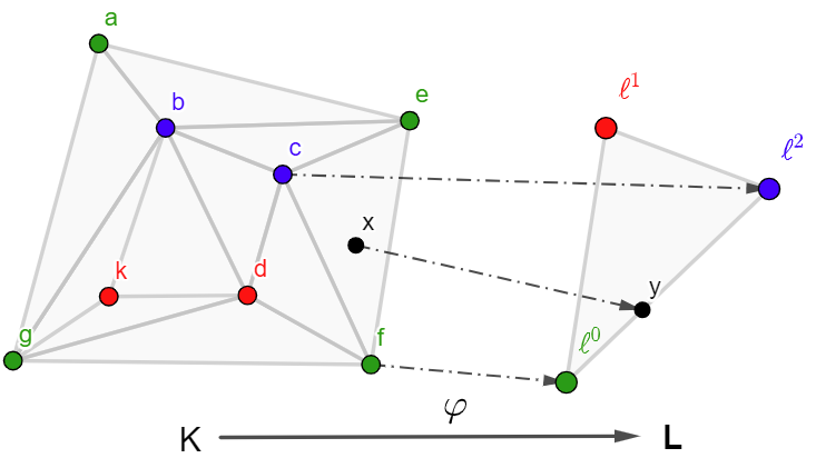
Figure 2: Illustration of a simplicial map for a classification task.

2.4 Simplicial map neural networks

Artificial neural networks can be seen as parametrized real-valued mappings between multidimensional spaces. Such mappings are the composition of several maps (usually many of them) that can be structured in layers. In [16], the simplicial map $\varphi$ defined above was represented as a two-hidden-layer feed-forward neural network $\mathcal{N}_{\varphi}$. This kind of network is the so-called simplicial map neural networks (SMNN).

In the original definition, the first hidden layer of SMNN computes the barycentric coordinates of $\operatorname{Del}(V\cup P)$. However, if we precompute these barycentric coordinates, we can remove the first hidden layer and simplify the architecture of $\mathcal{N}_{\varphi}$ as follows.

As before, consider an input dataset consisting of a finite set $V\subset\mathbb{R}^{n}$ endowed with a set of $k$ labels and a convex polytope $\mathcal{P}$ with a set of vertices $P$ surrounding $V$. Let $\operatorname{Del}(V\cup P)$ be the Delaunay triangulation with vertex set

$$V\cup P=\{\omega^{1},\dots,\omega^{\alpha}\}\subseteq\mathbb{R}^{n}\,.$$

Then, $\varphi^{\scriptscriptstyle(0)}:V\cup P\to W^{k+1}$ is a vertex map. Let us assume that, given $x\in\mathcal{P}$, we precompute the barycentric coordinates $b(x)=(b_{0}(x),\dots,b_{n}(x))\in\mathbb{R}^{n+1}$ of $x$ with respect to an $n$-simplex $\sigma=\langle\omega^{i_{0}},\dots,\omega^{i_{n}}\rangle\in\operatorname{Del}(V\cup P)$, and we have also precomputed the vector

$$\xi(x)=(\xi_{1}(x),\dots,\xi_{\alpha}(x))\in\mathbb{R}^{\alpha}$$

satisfying that, for $t\in[\![1,\alpha]\!]$, $\xi_{t}(x)=b_{j}(x)$ if $i_{j}=t$ for some $j\in[\![0,n]\!]$.

Then, the SMNN $\mathcal{N}_{\varphi}$ induced by $\varphi$ that predicts the $h$-label of $x$, for $h\in[\![0,k]\!]$, then has the following architecture:

• The number of neurons in the input layer is $\alpha$.

• The number of neurons in the output layer is $k+1$.

• The set of weights is represented as a $(k+1)\times\alpha$ matrix $\mathcal{M}$ such that the $j$-th column of $\mathcal{M}$ is $\varphi^{\scriptscriptstyle(0)}(\omega^{t})$ for $t\in[\![1,\alpha]\!]$.

Then,

$$\mathcal{N}_{\varphi}(x)=\max_{h\in[\![0,k]\!]}\mathcal{M}\cdot\xi(x)\,$$

SMNNs have several pros and cons. The advantages are that they are explainable (as we will see in Section 6), they can be transformed to be robust to adversarial examples [16] and their architecture can be reduced while maintaining accuracy [15]. Besides, they are invariant to transformation if the transformation preserves the barycentric coordinates (scale, rotation, symmetries, etc.).

Nevertheless, one drawback is that, as defined so far, the SMNN weights are untrainable, resulting in overfitting and reducing SMNN generalization capability. Furthermore, the computation of the barycentric coordinates of the points around $V$ implies the calculation of the convex polytope $\mathcal{P}$ surrounding $V$. Finally, the computation of the Delaunay triangulation $\operatorname{Del}(V\cup P)$ is costly if $V\cup P$ has many points, its time complexity is $O(n\log{n}+n^{\lceil\frac{d}{2}\rceil})$ (see [3, Chapter 4]).

In the next sections, we will propose some techniques to overcome the SMNN drawbacks while maintaining their advantages. We will see that one way to overcome the computation of the convex polytope $\mathcal{P}$ is to consider a hypersphere $S^{n}$ instead. We will also see how to avoid the use of the artificially created unknown label. Furthermore, to reduce the cost of Delaunay calculations and add trainability to $\mathcal{N}_{\varphi}$ to avoid overfitting, a subset $U\subset V$ will be considered. The set $V$ will be used to train and test a map $\varphi_{\scriptscriptstyle U}^{\scriptscriptstyle(0)}:U\to\mathbb{R}^{k}$. Such a map will induce a continuous function $\varphi_{\scriptscriptstyle U}:B^{n}\to|L|$ which approximates $\varphi$.

3 The unknown boundary and the function $\varphi_{\scriptscriptstyle U}$

In this section, We will see how to reduce the computation of the Delaunay triangulation used to construct SMNNs and will explain how to avoid the calculation of the convex polytope $\mathcal{P}$ and the consideration of the unknown label.

To reduce the cost of the Delaunay triangulation calculation and to add trainability to SMNNs to avoid overfitting, we will consider a subset $U=\{u^{1},\dots,u^{m}\}\subseteq V$. Furthermore, the set $U$ is translated so that its center of mass is placed at the origin $o\in\mathbb{R}^{n}$, and we will consider a hypersphere

$$S^{n}=\{w\in\mathbb{R}^{n}:\;||w||=R\}$$

satisfying that $R>\max\{||v||:\,v\in V\}$. Then,

$$V\subset B^{n}=\{x\in\mathbb{R}^{n}:\;||x||\leq R\}\;\mbox{ and }\;o\in|\operatorname{Del}(U)|\,.$$

Now, let us define and compute $\xi(x)\in\mathbb{R}^{m}$ for any $x\in B^{n}$ as follows.

First, let us consider the boundary of $\operatorname{Del}(U)$, denoted as $\delta\operatorname{Del}(U)$, which consists of the set of $(n-1)$-simplices that are faces of exactly one maximal simplex of $\operatorname{Del}(U)$.

Second, let $b(x)=(b_{0}(x),\dots,b_{n}(x))\in\mathbb{R}^{n+1}$ be the barycentric coordinates of $x$ with respect to some $n$-simplex $\sigma=\langle\omega^{0},\dots,\omega^{n}\rangle$, where $\sigma$ is computed as follows. If $x\in|\operatorname{Del}(U)|$ then $\sigma$ is an $n$-simplex of $\operatorname{Del}(U)$ such that $x\in|\sigma|$. Otherwise, $\sigma$ is a new $n$-simplex defined by the vertices of a simplex of $\delta\operatorname{Del}(U)$ and a new vertex consisting of the projection of $x$ to $S^{n}$. Specifically, if $x\not\in|\operatorname{Del}(U)|$ then $\sigma$ is computed in the following way:

1. Consider the set

   $$\Gamma=\big{\{}\mu\in\delta\operatorname{Del}(U):\;(N\cdot u^{i_{0}}+c)(N\cdot x+c)<0\big{\}}$$

   where $N$ is the normal vector to the hyperplane containing $\mu=\langle u^{i_{1}},\dots,u^{i_{n}}\rangle$, $c=N\cdot u^{i_{1}}$, and $u^{i_{0}}\in U$ such that $\langle u^{i_{0}},u^{i_{1}},\dots,u^{i_{n}}\rangle\in\operatorname{Del}(U)$.

2. Compute the point $w^{x}=R\frac{x}{||x||}\in S^{n}$.

3. Find $\sigma=\langle w^{x},u^{i_{1}},\dots,u^{i_{n}}\rangle$ such that

   $$\mu=\langle u^{i_{1}},\dots,u^{i_{n}}\rangle\in\Gamma\; \;x\in|\sigma|$$ and .

   Observe that, by construction, $\mu$ always exists since $|\operatorname{Del}(U)|$ is a convex polytope.

Then, $\xi(x)=(\xi_{1}(x),\dots,\xi_{m}(x))$ is the point in $\mathbb{R}^{m}$ satisfying that, for $t\in[\![1,m]\!]$,

$$\xi_{t}(x)=\left\{\begin{array}[]{cl}b_{j}(x)&\mbox{ if $u^{t}=\omega^{j}$ for some $j\in[\![0,n]\!]$, }\\ 0&\mbox{ otherwise.}\end{array}\right.$$

Observe that $\xi(x)$ always exists and is unique. An example of points $x$ and $w^{x}$ and simplex $\mu$ is shown in Figure 3.

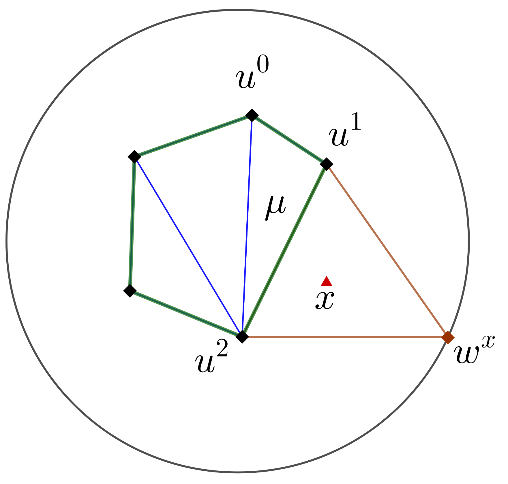
Figure 3: An example of the point $w^{x}$ computed from $x$ and the $(n-1)$-simplex $\mu=\langle u^{1},u^{2}\rangle\in\Gamma$ such that $x\in|\sigma|$ for $\sigma=\langle w^{x},u^{1},u^{2}\rangle$.

The following property holds.

Lemma 2 (Continuity)

Let $x\in B^{n}$. Then,

$$\lim_{y\to x}\xi(y)=\xi(x).$$

Proof. If $x\in|\operatorname{Del}(U)|$, then the result states due to the continuity of the barycentric coordinates transformation. If $x\not\in|\operatorname{Del}(U)|$, since $o\in|\operatorname{Del}(U)|$, then $||x||\neq 0$. Therefore, for $y$ close to $x$, $||y||\neq 0$ and $w^{y}=R\frac{y}{||y||}\in\mathbb{R}^{n}$. Besides,

$$\lim_{y\to x}w^{y}=w^{x}$$

and therefore

$$\lim_{y\to x}\xi(y)=\xi(x).$$

$\Box$

Let us observe that, thanks to the new definition of $\xi(x)$ for $x\in B^{n}$, if we have a map $\varphi_{\scriptscriptstyle U}^{\scriptscriptstyle(0)}:U\to\mathbb{R}^{k}$ then it induces a continuous function $\varphi_{\scriptscriptstyle U}:B^{n}\to|L|$ defined for any $x\in B^{n}$ as:

$$\varphi_{\scriptscriptstyle U}(x)=\operatorname{softmax}\big{(}\sum_{\scriptscriptstyle t\in[\![1,m]\!]}\xi_{t}(x)\varphi_{\scriptscriptstyle U}^{\scriptscriptstyle(0)}(u^{t})\big{)}$$

where for $z=(z_{1},\dots,z_{k})\in\mathbb{R}^{k}$,

$$\mbox{$\operatorname{softmax}(z)=\left(\frac{e^{z_{1}}}{\sum_{\scriptscriptstyle h\in[\![1,k]\!]}e^{z_{h}}},\dots,\frac{e^{z_{k}}}{\sum_{\scriptscriptstyle h\in[\![1,k]\!]}e^{z_{h}}}\right)$}.$$

The following result establishes that if the vertices of the convex polytope $\mathcal{P}$ are far enough from the vertices of $V$ and $\varphi_{\scriptscriptstyle U}^{\scriptscriptstyle(0)}(v)=\varphi^{\scriptscriptstyle(0)}(v)$ for all $v\in V$, then the behavior of $\varphi_{\scriptscriptstyle U}$ is the same as that of $\varphi$ inside $|\operatorname{Del}(V)|$.

Lemma 3 (Consistence)

Let $\varphi^{\scriptscriptstyle(0)}$ be the map defined in Subsection 2.3. If $U=V$, $\operatorname{Del}(V)\subseteq\operatorname{Del}(V\cup P)$ and $\varphi_{\scriptscriptstyle U}^{\scriptscriptstyle(0)}=\varphi^{\scriptscriptstyle(0)}|_{V}$ then

$$\varphi_{\scriptscriptstyle U}(x)=\varphi(x)\;\mbox{ for all }x\in\operatorname{Del}(V)\,.$$

Proof. Observe that if $U=V$, $\operatorname{Del}(V)\subseteq\operatorname{Del}(V\cup P)$ and $\varphi_{\scriptscriptstyle U}^{\scriptscriptstyle(0)}(v)=\varphi^{\scriptscriptstyle(0)}(v)$ for all $v\in V$ then, for any $x\in\operatorname{Del}(V)$, we have:

$$\varphi(x)=\sum_{\scriptscriptstyle t\in[\![1,m]\!]}\xi_{t}(x)\varphi^{\scriptscriptstyle(0)}(v^{t})=\sum_{\scriptscriptstyle t\in[\![1,m]\!]}\xi_{t}(x)\varphi_{\scriptscriptstyle U}^{\scriptscriptstyle(0)}(v^{t})$$.

Therefore, $\varphi_{\scriptscriptstyle U}(x)=\operatorname{softmax}\big{(}\varphi(x)\big{)}=\varphi(x)$. $\Box$

4 Measuring the similarity between $\varphi_{\scriptscriptstyle U}$ and $\varphi$

One of the keys to our study is the identification of the points of ${\mathbb{R}}^{n}$ allocated inside a given simplex with the set of all of the probability distributions with $n+1$ support values. In this way, the barycentric coordinates of a point can be seen as a probability distribution.

From this point of view, given $x\in B^{n}$, then $\varphi(x)$ and $\varphi_{\scriptscriptstyle U}(x)$ are both in the set $|L|$ of probability distributions with $k$ support points. This is why the categorical cross-entropy loss function $\mathcal{L}$ will be used to compare the similarity between $\varphi$ and $\varphi_{\scriptscriptstyle U}$. Specifically, for $v\in V$, $\mathcal{L}$ is defined as:

$$\mbox{$\mathcal{L}(\varphi_{\scriptscriptstyle U},\varphi,v)=-\sum_{\scriptscriptstyle h\in[\![1,k]\!]}y_{h}\log(s_{h})$}\,,$$

where $\varphi^{\scriptscriptstyle(0)}(v)=(y_{1},\dots,y_{k})$ and $\varphi_{\scriptscriptstyle U}(v)=(s_{1},\dots,s_{k})$.

The following lemma establishes a specific set $U\subset V$ and a function $\hat{\varphi}_{\scriptscriptstyle U}$ such that $\mathcal{L}(\varphi_{\scriptscriptstyle U},\varphi,v)=0$ is $0$ for all $v\in V$.

Lemma 4 ($\mathcal{L}$-optimum simplicial map)

Let $U\subseteq V$ such that for all $u\in U$, we have that $\hat{\varphi}_{\scriptscriptstyle U}^{\scriptscriptstyle(0)}(u)=\varphi^{\scriptscriptstyle(0)}(u)$ and there exists $v\in V\cup P$ with $\varphi^{(0)}(v)\neq\varphi^{(0)}(u)$ and $\langle v,u\rangle\in\operatorname{Del}(V)$. Then, $\mathcal{L}(\hat{\varphi}_{\scriptscriptstyle U},\varphi,v)=0$ for all $v\in V$.

Proof. As proved in [15], under the assumptions stated in this lemma, we have that $\varphi_{\scriptscriptstyle U}(v)=\varphi^{\scriptscriptstyle(0)}(v)$ for all $v\in V$ and then $\mathcal{L}(\varphi_{\scriptscriptstyle U},\varphi,v)=0$.

$\Box$

Unfortunately, to compute such $\hat{\varphi}_{\scriptscriptstyle U}$ we would need to compute the entire triangulation $\operatorname{Del}(U)$ which is computationally expensive, as we have already mentioned above.

This way, the novel idea of this paper is to learn the function ${\varphi}_{\scriptscriptstyle U}^{\scriptscriptstyle(0)}$ using gradient descent, in order to minimize the loss function $\mathcal{L}(\varphi_{\scriptscriptstyle U},\varphi,v)$ for any $v\in V$. The following result provides an expression of the gradient of $\mathcal{L}$ in terms of the functions $\varphi_{\scriptscriptstyle U}$ and $\varphi$, and the set $V$.

Theorem 1

Let $U=\{u^{1},\dots,u^{m}\}$ be a subset with $m$ elements taken from a finite set of points $V\in\mathbb{R}^{n}$ tagged with labels taken from a set of $k$ labels. Let $\varphi_{\scriptscriptstyle U}:B^{n}\to|L|$ and $\varphi^{(0)}:V\to W^{k}$. Let us consider that

$$\big{\{}\,\varphi_{\scriptscriptstyle U}^{\scriptscriptstyle(0)}(u^{t})=(p_{1}^{t},\dots,p_{k}^{t}):\;t\in[\![1,m]\!]\,\big{\}}$$

is a set of variables. Then, for $v\in V$,

$$\frac{\partial\mathcal{L}(\varphi_{\scriptscriptstyle U},\varphi,v)}{\partial p_{j}^{t}}=(s_{j}-y_{j})\xi_{t}(v)$$

where $j\in[\![1,k]\!]$, $t\in[\![1,m]\!]$, $\varphi^{(0)}(v)=(y_{1},\dots,y_{k})$ and $\varphi_{{\scriptscriptstyle U}}(v)=(s_{1},\dots,s_{k})$.

Proof. We have:

$$\frac{\partial\mathcal{L}(\varphi_{\scriptscriptstyle U},\varphi,v)}{\partial p_{j}^{t}} = -\frac{\partial\big{(}\sum_{h\in[\![1,k]\!]}y_{h}\;\log(s_{h})\big{)}}{\partial p_{j}^{t}}$$

$$= -\sum_{\scriptscriptstyle h\in[\![1,k]\!]}y_{h}\;\frac{\partial\log(s_{h})}{\partial p_{j}^{i}}$$

$$= \mbox{$-\sum_{\scriptscriptstyle h\in[\![1,k]\!]}y_{h}\;\frac{\partial\log(s_{h})}{\partial z_{j}}\frac{\partial z_{j}}{\partial p_{j}^{i}}$}\,.$$

Since $s_{h}=\frac{e^{z_{h}}}{\sum_{t\in[\![1,k]\!]}e^{z_{t}}}$ then

$$\frac{\partial\log(s_{h})}{\partial z_{j}} = \frac{\partial\log\big{(}\frac{e^{z_{h}}}{\sum_{t\in[\![1,k]\!]}e^{z_{t}}}\big{)}}{\partial z_{j}}$$

$$= \frac{\partial\log(e^{z_{h}})}{\partial z_{j}}-\frac{\partial\log\big{(}\sum_{t\in[\![1,k]\!]}e^{z_{t}}\big{)}}{\partial z_{j}}$$

$$= \frac{\partial z_{h}}{\partial z_{j}}-\frac{1}{\sum_{t\in[\![1,k]\!]}e^{z_{t}}}\;\sum_{\scriptscriptstyle t\in[\![1,k]\!]}\frac{\partial e^{z_{t}}}{\partial z_{j}}$$

$$= \mbox{$\delta_{hj}-\frac{e^{z_{j}}}{\sum_{t\in[\![1,k]\!]}e^{z_{t}}}$}=\delta_{hj}-s_{j}\,.$$

Besides, since $z_{j}=\sum_{\scriptscriptstyle h\in[\![1,m]\!]}\xi_{h}(v)p_{j}^{h}$ then

$$\mbox{$\frac{\partial z_{r}}{\partial p_{j}^{t}}=\sum_{h\in[\![1,m]\!]}\xi_{h}(v)\frac{\partial p_{r}^{h}}{\partial p_{j}^{t}}=\xi_{t}(v)$}\,.$$

Finally,

$$\frac{\partial\mathcal{L}(\psi,\varphi,v)}{\partial p_{j}^{t}} = -\sum_{\scriptscriptstyle h\in[\![1,k]\!]}y_{h}(\delta_{hj}-s_{j})\xi_{t}(v)$$

$$= -\xi_{t}(v)\big{(}\sum_{\scriptscriptstyle h\in[\![1,k]\!]}y_{h}\delta_{hj}-s_{j}\sum_{\scriptscriptstyle h\in[\![1,k]\!]}y_{h}\big{)}$$

$$= (s_{j}-y_{j})\xi_{t}(v)\,.$$

$\Box$

5 Training SMNNs

Let us see now how we add trainability to the SMNN $\mathcal{N}_{\varphi_{\scriptscriptstyle U}}$ induced by $\varphi_{\scriptscriptstyle U}$.

First, assuming that $U=\{u^{1},\dots,u^{m}\}$ has $m$ elements, then $\mathcal{N}_{\varphi_{\scriptscriptstyle U}}$ is a multiclass perceptron with an input layer with $m$ neurons that predicts the $h$-th label for $h\in[\![1,k]\!]$ using the formula:

$$\mathcal{N}_{\varphi_{\scriptscriptstyle U}}(x)=\max_{h\in[\![0,k]\!]}\;\operatorname{softmax}\big{(}\mathcal{M}\cdot\xi(x)\big{)}$$

where $\mathcal{M}=(p_{j}^{t})_{j\in[\![1,k]\!],t\in[\![1.m]\!]}$ is a matrix of weights and $\xi(x)\in\mathbb{R}^{m}$ is obtained from the barycentric coordinates of $x\in B^{n}$ as in Section 3. Let us observe that

$$\operatorname{softmax}\big{(}\mathcal{M}\cdot\xi(x)\big{)}\in|L|.$$

The idea is to modify the values of

$$\varphi^{\scriptscriptstyle(0)}_{\scriptscriptstyle U}(u^{t})=(p_{1}^{t},\dots,p_{k}^{t})\; u^{t}\in U t\in[\![1,m]\!]$$ for and ,

in order to obtain new values for $\varphi_{\scriptscriptstyle U}(v)$ in a way that the error $\mathcal{L}(\varphi_{\scriptscriptstyle U},\varphi,v)$ decreases. We will do it by avoiding recomputing $\operatorname{Del}(U)$ or the barycentric coordinates $(b_{0}(v),\dots,b_{n}(v))$ for each $v\in V$ during the training process.

This way, given $v\in V$, if $v\in|\operatorname{Del}(U)|$, we compute the maximal simplex $\sigma=\langle u^{i_{0}},\dots,u^{i_{n}}\rangle\in\operatorname{Del}(U)$ such that $v\in|\sigma|$ and $i_{h}\in[\![1,m]\!]$ for $h\in[\![0,n]\!]$. If $v\not\in|\operatorname{Del}(U)|$, we compute $w\in S^{n}$ and the simplex $\sigma=\langle w,u^{i_{1}},\dots,u^{i_{n}}\rangle$ such that $v\in|\sigma|$ and $i_{h}\in[\![1,m]\!]$ for $h\in[\![1,n]\!]$ Then, we compute the barycentric coordinates $b(v)$ of $v$ with respect to $\sigma$ and the point $\xi(x)=(\xi_{1}(x),\dots,\xi_{m}(x))\in\mathbb{R}^{m}$ as in Section 3.

Using gradient descent, we update the variables $p_{j}^{t}$ for $j\in[\![1,k]\!]$ and $t\in[\![1,m]\!]$ as follows:

$$p_{j}^{t}:=p_{j}^{t}-\eta\frac{\partial\mathcal{L}(\varphi_{\scriptscriptstyle U},\varphi,v)}{\partial p_{j}^{t}}=p_{j}^{t}-\eta(s_{j}-y_{j})\xi_{t}(v)$$.

6 Explainability

In this section, we provide insight into the explainability capability of SMNNs.

More specifically, explainability will be provided based on similarities and dissimilarities of the point $x$ to be explained with the points corresponding to the vertices of the simplex $\sigma$ containing it. Based on that, the barycentric coordinates of $x$ with respect to $\sigma$ can be considered indicators of how much a vertex of $\sigma$ is going to contribute to the prediction of $x$. Then, the multiplication of the barycentric coordinates of $x$ by the trained map $\varphi_{\scriptscriptstyle U}^{\scriptscriptstyle(0)}$ evaluated at the vertices of $\sigma$ is computed, and it provides the contribution of the labels assigned to each vertex of $\sigma$ after the training process to the label assigned to $x$ by the SMNN.

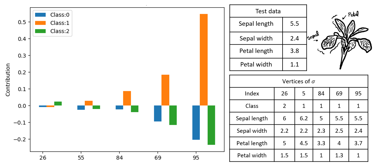
Figure 4: Table with the five flowers taken from the training set that influence the classification of a given flower in the test set, i.e. the vertices of $\sigma$.

As an illustration, let us consider the Iris dataset as a toy example and split it into a training set ($75\%$) and a test set ($25\%$). Since we focus on this section on explainability, let us take $U=V$, containing 112 points. Then, initialize $p_{j}^{t}$ with a random value in $[0,1]$, for $j\in[\![1,4]\!]$ and $t\in[\![1,112]\!]$.

After the training process, the SMNN reached $92\%$ accuracy on the test set. Once the SMNN is trained, we may be interested in determining why a certain output is given for a specific point $x$ in the test set.

As previously mentioned, the explanation of why the SMNN assigns a label to $x$ is based on the vertices of the simplex of $\operatorname{Del}(U)$ containing $x$. Therefore, the first step is to find the maximal simplex $\sigma$ that contains the point $x$ to be explained. As an example, in Figure 4, the point $x=(5.5,2.4,3.8,1.1)\in\mathbb{R}^{4}$ in the test set is chosen to be explained, predicted by the SMNN to class 2. The coordinates of the five vertices ($u^{26}$, $u^{55}$, $u^{69}$, $u^{84}$ and $u^{95}$) of the simplex $\sigma$ containing $x$ together with the classes they belong to are shown on the table at the bottom of Figure 4. The contribution of the class assigned to each vertex of $\sigma$ to the class assigned to $x$ by the SMNN is displayed in the bar chart, and is measured in terms of $\xi_{t}(x)\times p_{j}^{t}$ for $j\in[\![0,2]\!]$ and $t\in\{26,55,69,84,95\}$. We have noticed that the contributions can be positive or negative. For example, the vertex with the most influence in the classification affected negatively toward classifying the test data into the first class and third class, but positively towards the second class, which is the correct classification. Let us remark that Euclidean distance between points is not the only thing that makes higher the contribution of a vertex of $\sigma$. During the training process, the weights are adjusted considering the different simplices where that vertex belongs. Therefore, even if two points are equally close to the point to be explained, they will not contribute the same. In this example, the coordinates of vertices $84$ and $95$ are close to the test point but their contribution is very different in magnitude.

7 Experiments

In this Section, we provide experimentation showing the performance of SMNNs. SMNNs are applied to different datasets and compared with a feedforward neural network.

We split the given dataset into a training set composed of $75\%$ of the data and a test set of $25\%$. Then, the training set was used to train a feedforward neural network and an SMNN. In the case of SMNNs, a representative dataset (see [6]) of the training set was used as the $U$ support set. Let us now describe the methodology more specifically for each dataset used.

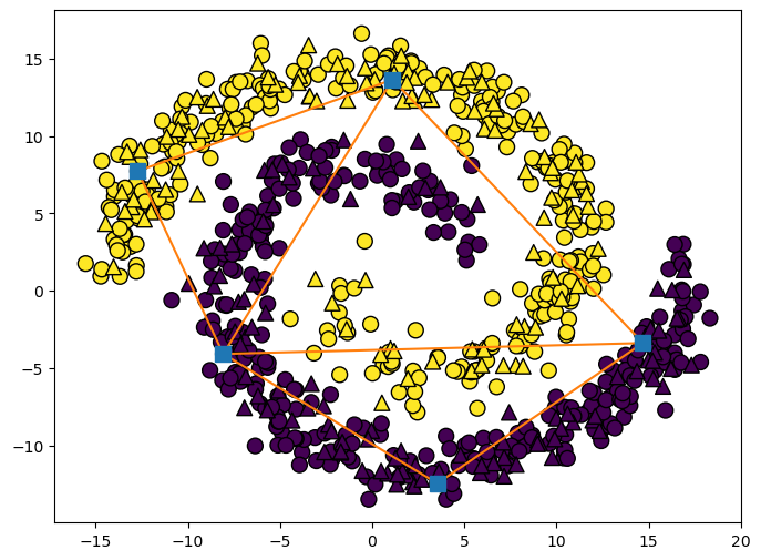
(a) Using $5$ support points. The SMNN reaches $80\%$ of accuracy on the test set.

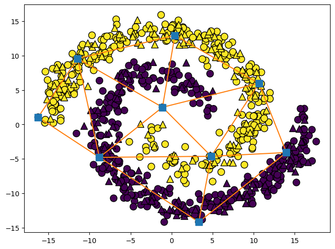
(b) Using $9$ support points. The SMNN reaches $93\%$ of accuracy on the test set.

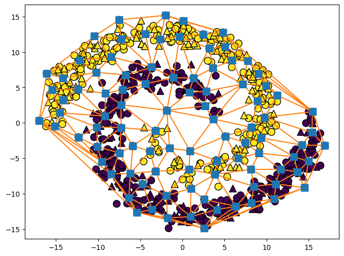
(c) Using $95$ support points. The SMNN reaches $99\%$ of accuracy on the test set.

Figure 5: Spiral dataset for binary classification. On each figure, the support points are the squared-shaped points, the test data is triangle-shaped and the training data is circle-shaped.

The first dataset used for visualization purposes is a spiral dataset composed of $400$ two-dimensional points, in Figure 5, it shows different sizes of the support subset together with the associated Delaunay triangulation. As can be seen, in this case, the accuracy increases with the size of the support subset. We can also appreciate that the topology of the dataset is characterized by the representative support set leading to successful classification.

The second datasets are synthetic datasets of size $5000$ the Scikit-learn implementation. See Figure 6 where a small two-dimensional example is shown. The datasets generated have from $2$ to $5$ features and results are provided in Table 1. SMNNs were trained using the gradient descent algorithm and the cross-entropy loss function during $500$ epochs, and using different representative parameters to choose the support set $U$. Then, a two-hidden-layer feedforward ($32\times 16$) neural network with ReLu activation functions was trained using the same datasets using Adam training algorithm. The results provided are the mean of $100$ repetitions. In Table 1, we can see that both neural networks had similar performance, but SMNNs generally reach lower loss. The variance in the results was of the order of $10^{-8}$ to $10^{-5}$ in the case of SMNNs and of $10^{-5}$ to $10^{-2}$ in the case of the feedforwad neural network.

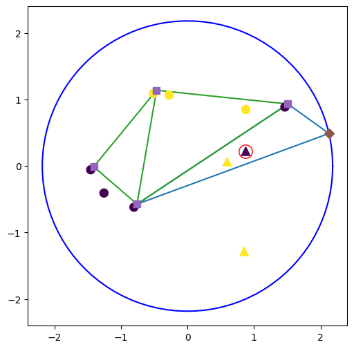
Figure 6: Two-dimensional binary classification synthetic dataset. Classes: Blue and yellow. Triangle-shaped points are test data and square-shaped points are representative points used for training. The diamond-shaped point is the vertex on the hypersphere (the blue circumference) used to classify the test point (surrounded by red circumference) outside the triangulation.

	SMNN				NN
$n$	$\varepsilon$	$m$	Acc.	Loss	Acc.	Loss
2	1000	3560	0.87	0.64	0.91	0.23
	100	1282	0.90	0.51
	50	626	0.9	0.42
	10	53	0.87	0.33
3	1000	3750	0.76	0.66	0.8	0.61
	100	3664	0.76	0.66
	50	3252	0.77	0.65
	10	413	0.81	0.5
4	50	3728	0.69	0.67	0.72	0.69
	10	1410	0.73	0.64
	5	316	0.73	0.57
	2	26	0.72	0.56
5	50	3743	0.77	0.66	0.8	0.91
	10	1699	0.81	0.63
	5	323	0.8	0.52
	2	17	0.74	0.53

Table 1: Accuracy score and loss values obtained after training both an SMNN and a feedforward neural network. The experiments were repeated $100$ times and the results provided are the mean of the accuracy values of the repetitions. The size $m$ of the subset considered to compute the Delaunay triangulation also varies in each experiment depending of a representation parameter which is the maximum distance from the origin to the further point in the dataset plus $\frac{1}{2}$ and divided by the value provided in the column $\varepsilon$. The feedforward neural network is composed of two hidden layers of size $32$ and $16$, respectively, with ReLu activation functions and an output layer with a softmax activation function. The datasets used are synthetic datasets for binary classification with numbers of features $n$.

8 Conclusions

Simplicial map neural networks provide a combinatorial approach to artificial intelligence. Its simplicial-based definition provides nice properties such us easy construction, and robustness capability against adversarial examples. In this work, we have extend its definition to provide a trainable version of this architecture and exploited its explainability capability.

In this paper, we only applied standard training algorithms to study its performance. As future work, it would be interesting to study different kind of training algorithms and choices of the support set. In addition, studies towards seeking more efficient implementations to avoid Delaunay triangulations should be performed.

Supplementary material

Code with the experiments and an illustrative jupyter notebook are provided as supplementary material with this submission.

9 Aknowledgments

The work was supported in part by European Union HORIZON-CL4-2021-HUMAN-01-01 under grant agreement 101070028 (REXASI-PRO), and by AEI/10.13039/501100011033 under grants PID2019-107339GB-100 and TED2021-129438B-I00/Unión Europea NextGenerationEU/PRTR.

References

- [1] Gulsum Alicioglu and Bo Sun. A survey of visual analytics for explainable artificial intelligence methods. Computers and Graphics, 102:502–520, Feb. 2022.
- [2] Katie Atkinson, Trevor J. M. Bench-Capon, and Danushka Bollegala. Explanation in AI and law: Past, present and future. Artif Intell, 289:103387, 2020.
- [3] Jean-Daniel Boissonnat, Frédéric Chazal, and Mariette Yvinec. Geometric and Topological Inference. Cambridge Texts in Applied Maths. Cambridge Univ Press, 2018.
- [4] Juan M. Durán. Dissecting scientific explanation in AI (sxai): A case for medicine and healthcare. Artif Intell, 297:103498, 2021.
- [5] Herbert Edelsbrunner and John Harer. Computational Topology - an Introduction. Am Math Soc, 2010.
- [6] Rocio Gonzalez-Diaz, Miguel A. Gutiérrez-Naranjo, and Eduardo Paluzo-Hidalgo. Topology-based representative datasets to reduce neural network training resources. Neural Comput. Appl., 34(17):14397–14413, 2022.
- [7] Mara Graziani, Lidia Dutkiewicz, Davide Calvaresi, and et al. A global taxonomy of interpretable ai: unifying the terminology for the technical and social sciences. Artif Intell Rev, 2022.
- [8] Arjan M. Groen, Rik Kraan, Shahira F. Amirkhan, Joost G. Daams, and Mario Maas. A systematic review on the use of explainability in deep learning systems for computer aided diagnosis in radiology: Limited use of explainable ai? European Journal of Radiology, 157:110592, 2022.
- [9] Vinay Jogani, Joy Purohit, Ishaan Shivhare, and Seema C Shrawne. Analysis of explainable artificial intelligence methods on medical image classification. arXiv, 2022.
- [10] Hassan Khosravi, Simon Buckingham Shum, Guanliang Chen, Cristina Conati, Yi-Shan Tsai, Judy Kay, Simon Knight, Roberto Martínez Maldonado, Shazia Wasim Sadiq, and Dragan Gasevic. Explainable artificial intelligence in education. Comput Educ Artif Intell, 3:100074, 2022.
- [11] Hui Wen Loh, Chui Ping Ooi, Silvia Seoni, Prabal Datta Barua, Filippo Molinari, and U. Rajendra Acharya. Application of explainable artificial intelligence for healthcare: A systematic review of the last decade (2011-2022). Comput Methods Programs Biomed, 226:107161, 2022.
- [12] Christoph Molnar. Interpretable Machine Learning. Independently published, 2 edition, 2022.
- [13] W. James Murdoch, Chandan Singh, Karl Kumbier, and et al. Definitions, methods, and applications in interpretable machine learning. PNAS, 2019.
- [14] Eduardo Paluzo-Hidalgo, Rocio Gonzalez-Diaz, and Miguel A. Gutiérrez-Naranjo. Two-hidden-layer feed-forward networks are universal approximators: A constructive approach. Neural Netw, 131:29–36, 2020.
- [15] Eduardo Paluzo-Hidalgo, Rocio Gonzalez-Diaz, Miguel A. Gutiérrez-Naranjo, and Jónathan Heras. Optimizing the simplicial-map neural network architecture. J Imaging, 7(9):173, 2021.
- [16] Eduardo Paluzo-Hidalgo, Rocio Gonzalez-Diaz, Miguel A. Gutiérrez-Naranjo, and Jónathan Heras. Simplicial-map neural networks robust to adversarial examples. Mathematics, 9(2):169, 2021.
- [17] Marco Tulio Ribeiro, Sameer Singh, and Carlos Guestrin. ”why should i trust you?”: Explaining the predictions of any classifier. In Proc of the 22nd ACM SIGKDD Int. Con. on Knowledge Discovery and Data Mining, KDD ’16, page 1135–1144. Assoc. for Computing Machinery, 2016.