Detecting Heart Disease from Multi-View Ultrasound Images via Supervised Attention Multiple Instance Learning

Abstract

Aortic stenosis (AS) is a degenerative valve condition that causes substantial morbidity and mortality. This condition is under-diagnosed and under-treated. In clinical practice, AS is diagnosed with expert review of transthoracic echocardiography, which produces dozens of ultrasound images of the heart. Only some of these views show the aortic valve. To automate screening for AS, deep networks must learn to mimic a human expert’s ability to identify views of the aortic valve then aggregate across these relevant images to produce a study-level diagnosis. We find previous approaches to AS detection yield insufficient accuracy due to relying on inflexible averages across images. We further find that off-the-shelf attention-based multiple instance learning (MIL) performs poorly. We contribute a new end-to-end MIL approach with two key methodological innovations. First, a supervised attention technique guides the learned attention mechanism to favor relevant views. Second, a novel self-supervised pretraining strategy applies contrastive learning on the representation of the whole study instead of individual images as commonly done in prior literature. Experiments on an open-access dataset and an external validation set show that our approach yields higher accuracy while reducing model size.

[sections]

1 Introduction

Aortic stenosis (AS) is a progressive degenerative valve condition that is the result of fibrotic and calcific changes to the heart valve. These structural changes occur over years and eventually lead to obstruction of blood flow, symptoms and death if not treated. AS is common and affects over 12.6 million adults and causes an estimated 102,700 deaths annually. AS can be effectively treated when it is identified in a timely manner though diagnosis remains challenging (Yadgir et al., 2020). One promising route to improving AS detection is to consider automatic screening of patients at risk using cardiac ultrasound. Automatic screening could provide a systematic, reproducible process and augment current approaches that rely on cardiac auscultation and miss a significant number of cases (Gardezi et al., 2018).

(a) Human expert approach		(b) Filter then Average (Holste et al., 2022b)
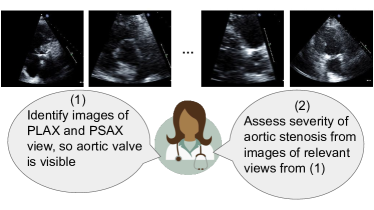
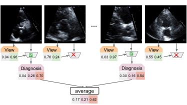
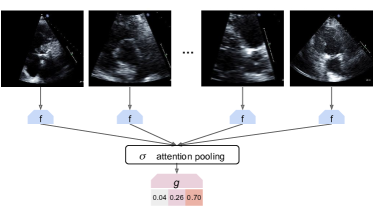
(c) Weighted Average by View Relevance (Wessler et al., 2023; Huang et al., 2021)		(d) Attention-based MIL

Figure 1: Overview of methods for diagnosing aortic valve disease from multiple images of the heart. In our chosen diagnostic problem, the input is multiple ultrasound images representing different canonical view types of the heart’s complex anatomy (e.g. PLAX, PSAX, A2C, A4C, and more, see Mitchell et al. (2019) for a taxonomy). The required output is a (probabilistic) prediction of the severity of Aortic Stenosis (AS), on a 3-level scale of no / early / significant disease. We wish to develop deep learning methods that can solve this problem like expert cardiologists (panel a). Two recent efforts (panel b by others, panel c by our group) made progress using a separately-trained view type classifier and per-image diagnosis classifier, but rely on combining diagnosis probabilities across images via average pooling that cannot learn how to distribute attention non-uniformly among images of relevant views. In this work, we develop more flexible attention-based multiple instance learning architectures (MIL, panel d), with crucial contributions of supervised attention (Sec. 4.3) and improved pretraining strategies (Sec. 4.4) that we show later yield substantially improved performance on this task.

The challenge in developing a robust automated system for diagnosing AS is that echocardiogram studies consist of dozens of images or videos that show the heart’s complex anatomy from many different acquisition angles. As illustrated in Fig. 1 (a), clinical readers are trained to look across many images to identify those that show the aortic valve at sufficient quality and then use these “relevant” images to assess the valve’s health. Training an algorithm to mimic this expert human diagnostic process is difficult. Most standard deep learning classifiers are designed to consume only one image and produce one prediction. Automatic screening of echocardiograms requires the ability to make one coherent prediction from many images representing diverse view types. To make matters more difficult, each image’s view type is not recorded in the EHR during routine collection.

Multiple-instance learning (MIL) is a branch of weakly supervised learning in which classifiers can consume a variable-sized set of images to make one prediction. Recent impressive advances in MIL have been published  (Ilse et al., 2018; Lee et al., 2019; Sharma et al., 2021; Shao et al., 2021). However, their success on ultrasound tasks, especially those with images from many possible view types, has not been carefully evaluated.

Contributions to clinical translation and MIL methodology

This study’s contribution to applied clinical research is the development and validation of a new deep MIL approach for automatic diagnosis of heart valve disease from multiple ultrasound images produced by a routine trans-thoracic echocardiogram (TTE) study. Our end-to-end approach can take as input any number of images from various view types. Our approach eliminates the need for a separately-trained filtering step (Fig. 1 (b)) to select relevant views for diagnosis, as required by some prior AS screening methods  (Holste et al., 2022b). Our approach is also more flexible and data-driven than the weighted average (Fig. 1 (c)) of other previous efforts of AS screening (Huang et al., 2021; Wessler et al., 2023). Head-to-head evaluation in Sec. 5 demonstrates that our approach can yield superior balanced accuracy for assigning AS severity grades to new studies, while keeping model size over 4x smaller than previous efforts like (Holste et al., 2022b). Small model sizes enable faster predictions and ease portability to new hospital systems.

Our approach’s success is made possible by two methodological contributions. First, we propose a supervised attention mechanism (Sec. 4.3) that steers focus toward images of relevant views, mimicking a human expert. On our AS diagnosis task, supervised attention yields notable gains – balanced accuracy jumps from 60% to over 70% – over previous off-the-shelf attention-based MIL (Ilse et al., 2018). Second, we introduce a self-supervised pretraining strategy (Sec. 4.4) that focuses contrastive learning on the embedding of an entire study (a.k.a. the embedding of the “bag”, using MIL vocabulary). In contrast, most previous pretraining focuses on representations of individual images. Both innovations are broadly applicable to other MIL problems involving imaging data of multiple view types.

Generalizable Insights about Machine Learning in the Context of Healthcare

This study offers critical insight into how multiple-instance learning can be applied to routine echocardiography studies. We show that recent MIL architectures are insufficient in achieving competitive performance and lack the ability to make clinically plausible decision (they attends to irrelevant instances). Our two innovations – supervised attention (Sec. 4.3) and bag-level self-supervised pretraining (Sec. 4.4.) can be broadly applicable to many clinical image analysis problems that require non-trivial aggregation over multiple images from multiple acquisition angles (views) to make one diagnosis. Beyond echocardiography, these insights could be useful for lung ultrasound, fetal ultrasound, head CT, and more.

2 Related Work

2.1 Multiple-instance learning.

Multiple-instance learning (Dietterich et al., 1997; Maron and Lozano-Pérez, 1997) describes a type of problem where an unordered bag of instances and their corresponding bag label are provided as input, and the goal is to predict the bag label for unseen bags. This type of problem appears in many medical applications, including whole-slide image (WSI) analysis in pathology  (Cosatto et al., 2013; Shao et al., 2021; Li et al., 2021a), diabetic retinopathy screening  (Quellec et al., 2012; Li et al., 2021c, d; Kandemir and Hamprecht, 2015), bacteria clones identification  (Borowa et al., 2020), drug activity prediction (Dietterich et al., 1997; Zhao et al., 2013), and cancer diagnosis  (Campanella et al., 2019; Chikontwe et al., 2020; Hou et al., 2016; Ding et al., 2012; Xu et al., 2014). Extensive reviews of the MIL literature are available (Zhou, 2004; Quellec et al., 2017; Carbonneau et al., 2018).

Two primary ways for modeling multiple instance learning problems are the instance-based approach and the embedding-based approach. In the instance-based approach, an instance classifier is used to score each instance, and a pooling operator is then used to aggregate the instance scores to produce a bag score. In the embedding-based approach, a feature extractor generates an embedding for each instance, which is then aggregated into a bag-level embedding. A bag-level model is subsequently employed to compute a bag score based on the embedding. The embedding-based approach is argued to deliver better performance than the instance-based approach (Wang et al., 2018), but at the same time harder to determine the key instances that trigger the classifier (Liu et al., 2017).

Deep attention-based MIL.

Our proposed method builds upon recent works advancing attention-based deep neural networks for MIL. (A broader summary of classic MIL can be found in App E). ABMIL (Ilse et al., 2018) is an embedding approach where a two-layer neural network computes attention weights for each instance, with the final representation formed by averaging over instance embeddings weighted by attention. Set Transformer (Lee et al., 2019) proposed to model the interactions among instances by using self-attention with multi-head attention (Vaswani et al., 2017). Similarly, TransMIL  (Shao et al., 2021) uses a Transformer-based architecture to capture correlations among patches for whole-slide image classification. C2C (Sharma et al., 2021) divides patches from a whole-slide image into clusters, and sample multiple patches from each cluster for training. C2C then tries to guide attention weights to be similar to a predefined uniform distribution, aiming to minimize intra-cluster variance for patches from the same cluster. A recent method called DSMIL (Li et al., 2021a) attempts to benefit from instance-based and embedding-based approaches via a dual-stream architecture. The author pretrains the instance-level feature extractor using self-supervised contrastive learning.

2.2 Self-supervised learning and Pretraining of MIL

Self-supervised learning (SSL) has demonstrated success in learning visual representations  (Oord et al., 2018; Chen et al., 2020a; He et al., 2020; Chen et al., 2020b; Grill et al., 2020; Caron et al., 2020; Chen and He, 2021). SSL requires defining a pretext task such as predicting the future in latent space (Oord et al., 2018), predicting the rotation of an image  (Gidaris et al., 2018), or solving a jigsaw puzzle (Noroozi and Favaro, 2016). The term ”pretext” suggests that the task being solved is not of genuine interest, but rather serves as a means to learn a better data representation. After selecting a pretext task, an appropriate loss function must also be selected. Here, we focus on the instance discrimination task (Wu et al., 2018) and InfoNCE loss (Oord et al., 2018) following the success of momentum contrastive learning (MoCo)  (He et al., 2020; Chen et al., 2020b).

Recently, self-supervision has been successfully applied to pretrain MIL models (Holste et al., 2022a, b; Liu et al., 2022; Lu et al., 2019; Li et al., 2021a; Saillard et al., 2021; Dehaene et al., 2020; Rymarczyk et al., 2023). However, these studies all apply self-supervised contrastive learning to representations of individual images. In our experiments, we observe image-level pretraining is not beneficial and sometimes slightly harmful for our AS diagnosis task. This may be because the pretraining task’s objective (learning good image level representations) being too distant from (or even contradict) the downstream task’s objective (learning good bag-level representations for AS diagnosis). This could relate to an issue prior literature calls class collision (Arora et al., 2019; Chuang et al., 2020; Khosla et al., 2020; Dwibedi et al., 2021; Zheng et al., 2021; Ash et al., 2021; Li et al., 2021b).

2.3 Applications of ML to Aortic Stenosis.

Work on automatic screening for aortic stenosis from echocardiograms has accelerated in the past few years. These efforts differ in how they overcome the challenge of multi-view images available in each patient scan or study.

Some groups have taken the Filter then Average approach diagrammed in Fig. 1 (b). Dai et al. (2023) used a single video of the PLAX view to screen for AS. Holste et al. (2022b) similarly filters to several PLAX videos, then uses a deep learning architecture specialized to video. This latter study reports strong external validation performance.

Another group pursued the Weighted Avg. by View Relevance strategy, shown in Fig. 1 (c). Huang et al. (2021) developed an approach for handling diverse views by combining an image-level view classifer and an image-level diagnosis classifier. This was later developed for a clinical audience in Wessler et al. (2023).

Very recent work by Krishna et al. (2023) demonstrated that a commercial deep learning system can closely emulate human performance on most of the elementary echocardiogram-derived measures for AS assessment, such as aortic valve area, peak velocity of blood through the valve, and mean pressure gradients. However, the inability to assign a study-level AS severity rating limits its usefulness as a screening tool.

More distant work has pursued automated AS screening beyond echo images. Some have created classifiers based on time-varying electrocardiogram signals (Cohen-Shelly et al., 2021; Elias et al., 2022). Others have used wearable sensors (Yang et al., 2020). We argue that 2D echocardiograms remain the gold-standard information source for diagnosis.

Overall, the use of video, rather than still frames, is an advantage of some prior work (Dai et al., 2023; Holste et al., 2022b) over our approach. However, these video works evaluate on proprietary data, while our current work emphasizes reproducibility by using the open-access TMED dataset described below. We expect our proposed MIL architecture could be extended to video by a straightforward adaptation of the instance representation layer.

3 Dataset

In this work, for model training and primary evaluation we use an open-access dataset that our team created. The Tufts Medical Echocardiogram Dataset (TMED) (Huang et al., 2021), now in its latest version known as TMED-2 (Huang et al., 2021), is a collection of 2D echocardiogram images gathered during routine care at Tufts Medical Center in Boston, MA, USA from 2016-2021. Our research study of these fully deidentified images has been approved by the Tufts Medical Center institutional review board.

Each study in the dataset represents a routine TTE scan of one patient and includes all collected 2D ultrasound images of the heart, with a median of $K=68$ images per study (10-90th percentile range = 27-97). No filtering to specific views was applied except removal of Doppler images via metadata inspection. Each study’s available set of images is exactly the set of 2D TTE images an expert cardiologist would see in the health records system.

TMED-2 contains a labeled set of 599 studies. Every study in the labeled set has a diagnosis label indicating the severity of AS observed. We use 3 severity levels: no AS, early AS, or significant AS. These are assigned by a board-certified expert during routine reading. We note that expert readers have access to more information than our algorithms: in addition to the 2D images, clinician readers also see Doppler images of blood flow as well as other clinical variables not available in TMED-2.

To make the most of the available data, we follow the recommended protocol of averaging over 3 separate predefined training/validation/test splits. Each split consists of 360/119/120 studies, constructed to yield similar proportions of no, early, and signficant AS.

View labels for view classifiers. A subset of images in the TMED-2 labeled set (around 40%) are labeled with view type. There are 5 possible view labels: { PLAX, PSAX, A2C, A4C, other}. Only PLAX and PSAX views show the aortic valve and thus are relevant for AS severity assessment. As per Mitchell et al. (2019), there are at least 9 canonical view types in routine TTEs, so many images in TMED-2 depict views that are “irrelevant” for AS diagnosis. View type labels are useful for training view classifiers. Our MIL approach does not need these view labels at all, only a pre-trained view classifier.

Unlabeled set for pretraining. TMED-2 additionally makes available a large unlabeled set of 5486 studies from distinct patients. Studies in the unlabeled set have no diagnosis label nor view label. We use this unlabeled set for pretraining representations, but cannot use them for the supervised training of our MIL due to the lack of labels.

2022-Validation dataset. For further evaluation, we obtained (with IRB approval) additional deidentified images from routine TTEs of 323 patients at our institution, collected during 2022 and assigned the same severity labels for AS as TMED-2 by a clinical expert during routine care. We call this data 2022-Validation. It contains 225/48/50 examples of no/early/significant AS.

4 Methods

We now introduce our formulation of AS diagnosis as an MIL problem in Sec 4.1 and discuss a general architecture for MIL (Sec. 4.2). We then present the two key innovations of our proposed method, which we call Supervised Attention Multiple Instance Learning or SAMIL. First, Sec. 4.3 presents our supervised attention module that improves the MIL pooling layer to better attend to clinically relevant views. Second, Sec. 4.4 presents our study-level contrastive learning strategy to improve representation of entire studies (rather than individual images). Fig 2 gives an overview of SAMIL.

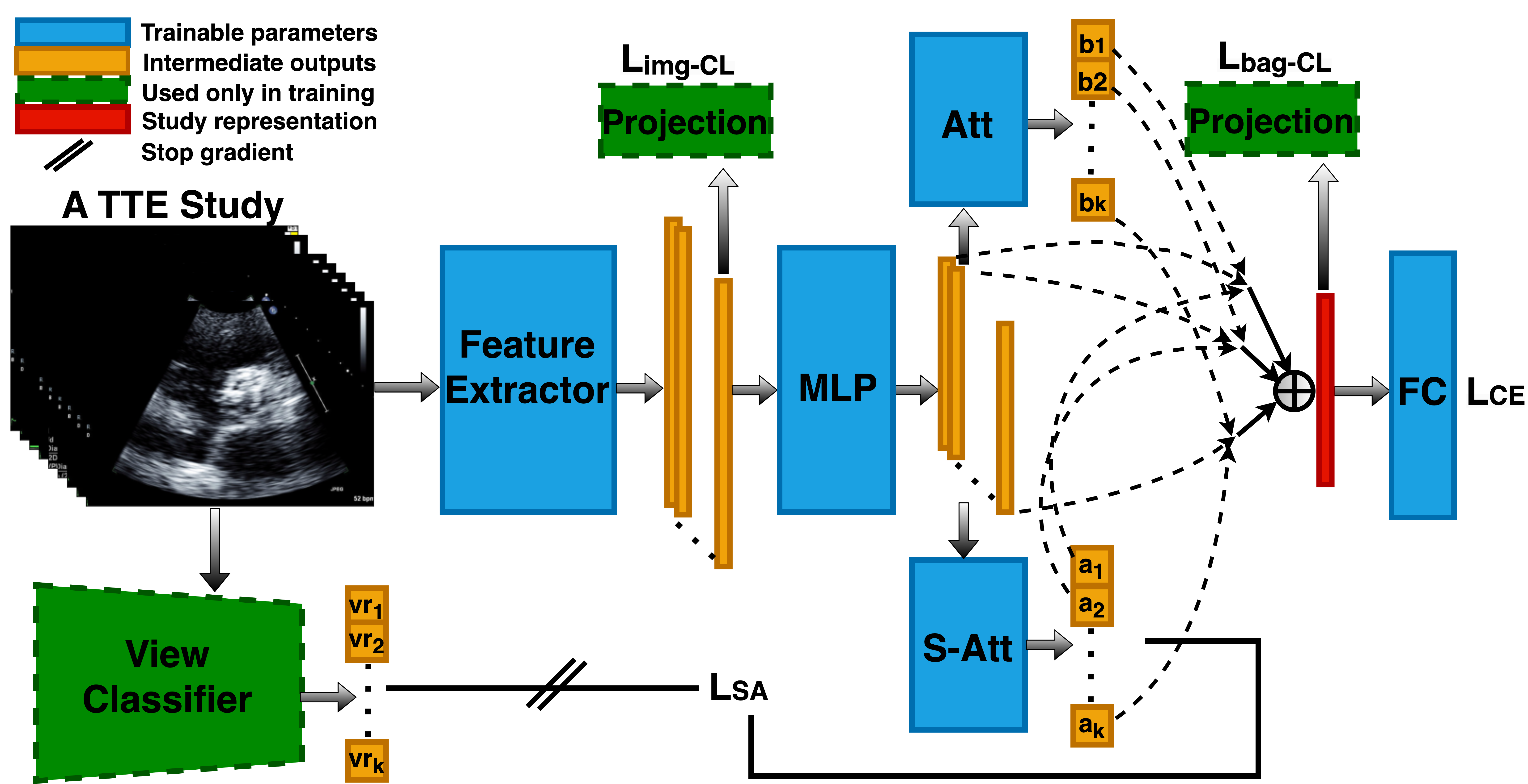
Figure 2: Overview of proposed method: Supervised Attention Multiple Instance Learning (SAMIL). Given a study or “bag” with various images, a feature extractor processes each image individually into an embedding vector. Two attention modules (one supervised by a trained view classifier and one without) produce attention weights for each instance. The final study representation averages the image embeddings weighted by a combination of the two attentions (Eq. (5)). A fully connected layer then maps the study representation to a diagnosis label. Pretraining: SAMIL can be pretrained using either bag-level (recommended, Sec. 4.4) or image-level contrastive learning. In either case, a projection head maps representations to a latent space where the contrastive loss is applied, following (Chen et al., 2020a, b). The projection head is discarded after pretraining.

4.1 Problem Formulation

Let $D=\{(X_{1},Y_{1}),\ldots,(X_{N},Y_{N})\}$ be a training dataset containing $N$ TTE studies. Each study, indexed by $i$, consists of a bag of images $X_{i}$ and an (optional) diagnostic label $Y_{i}$.

Prediction task. Given a training set of size $N$, our goal is to build a classifier that can consume a new echo study $X_{*}$ and assign the appropriate label $Y_{*}$.

Input. Each “bag” $X_{i}$ contains $K_{i}$ distinct images: $\{x_{i1},x_{i2},\ldots,x_{iK_{i}}\}$. These images represent all 2D TTE images gathered during a routine echocardiogram. The number of images $K_{i}$ varies across studies (typical range 27-97). Each image $x_{ik}$ is a grayscale image of 112x112 pixels.

Output. Each study’s diagnostic label $Y_{i}\in\{0,1,2\}$ indicates the assessed severity level of aortic stenosis (0 = no AS, 1 = early AS, 2 = significant AS). These labels are assigned by a cardiologist with specialty training in echocardiography during a routine clinical interpretation of the entire study. Diagnosis labels for individual images are unavailable.

Image preprocessing. We used the released dataset directly without additional preprocessing. As documented in Huang et al. (2022), the images are extracted from raw DICOM files in the health record by taking the first frame of the corresponding cineloop, removing identifying information, converted to grayscale, padding the shorter axis to a square aspect ratio, and resizing to 112x112.

4.2 General MIL architecture

Following past work on deep neural network approaches to MIL (Ilse et al., 2018; Li et al., 2021a), a typical architecture has 3 components, as illustrated in Fig. 1(d). First, an instance representation layer $f$ transforms each instance into a feature representation. Second, a pooling layer $\sigma$ aggregates across instances to form a bag-level representation in permutation-invariant fashion. Finally, an output layer $g$ maps the bag-level representation to a prediction.

We now describe the forward prediction process of one study or “bag” $X$ under this 3 component architecture when specialized to our AS severity prediction problem. Let $X=\{x_{1},\ldots,x_{K}\}$ be the input bag of K instances, with individual instances indexed by integer $k$. (We use $X$ interchangably with $X_{i}$ here, dropping the study-specific index $i$ to reduce notational clutter.)

Instance representation layer $f$.

Let $f$ be a row-wise feedforward layer that processes each instance $x_{k}\in\mathcal{X}$ independently and identically, producing an instance-specific embedding $h_{k}=f(x_{k})$, where $h_{k}\in\mathbb{R}^{M}$. Concretely, we use a stack of convolution layers and a MLP layer to extract and project the instance’s feature representation to low-dimensional embedding. More details in App. B.1.

Pooling layer $\sigma$.

ABMIL uses an attention-based pooling method which produces a bag-level representation $z\in\mathbb{R}^{M}$ via an attention-weighted average of the $K$ instance embeddings $\{h_{1},\ldots h_{K}\}$:

$$z=\sum_{k=1}^{K}a_{k}h_{k},\quad a_{k}=\frac{\exp(w^{\top}\tanh(Uh_{k}))}{\sum_{j=1}^{K}\exp(w^{\top}\tanh(Uh_{j}))},$$ (1)

where vector $w\in\mathbb{R}^{L}$ and matrix $U\in\mathbb{R}^{L\times M}$ are trainable parameters of layer $\sigma$. Alternative gated attention modules are also possible, but they tend to yield only marginal gains in classification performance.

Output layer $g$.

Given a bag-level feature vector $z=\sigma(f(X))$, the output layer performs probabilistic classification for the 3 levels of AS severity (0=none, 1=early, 2=significant) via a standard linear-softmax transformation of $z$:

$$p(Y=r|X)=g(z)_{r}~{}\text{for}~{}r\in\{0,1,2\},\qquad g(z)=\left[\frac{\exp(\eta_{0}^{\top}z)}{S(\eta,z)},\frac{\exp(\eta_{1}^{\top}z)}{S(\eta,z)},\frac{\exp(\eta_{2}^{\top}z)}{S(\eta,z)}\right].$$ (2)

Here, $\eta_{0},\eta_{1},\eta_{2}$ represent weights for each of the 3 severity levels of AS, and denominator $S=\sum_{r=0}^{2}\exp(\eta_{r}^{\top}z)$ ensures the probabilities sum to one. We do include an intercept term for each class, but omit from notation for clarity.

Training.

This 3-component deep MIL architecture has parameters $\eta$ for the output layer as well as $\theta$ for the pooling and representation layers ($\theta$ includes $w,U$ from Eq. (1)). We train these parameters by minimizing the cross-entropy loss between each study’s observed AS diagnosis $Y$ and the MIL-predicted probabilities given each bag of images $X$

$$\theta^{*},\eta^{*}=\arg\!\min_{\theta,\eta}\sum_{X,Y\in\mathcal{D}}\mathcal{L}_{\text{CE}}\left(Y,g_{\eta}(\sigma_{\theta}(f_{\theta}(X))\right)$$ (3)

In practice, weight decay is often used to regularize the model and improve generalization.

4.3 Contribution 1: Attention supervised by a view classifier

We find the attention-based architecture described above yields unsatisfactory performance in our diagnostic task (see table 1). Furthermore, the learned attention values used in Eq. (1) do not pass a clinical sanity check: attention should be paid only to PLAX and PSAX AoV view types, as only these show the aortic valve (see fig 3).

This last observation suggests a path forward: supervising the attention mechanism. Suppose we have access to a trustworthy view-type-relevance classifier $v:\mathcal{X}\rightarrow[0.0,1.0]$, which maps an image to the probability that it shows a relevant view depicting the aortic valve (either a PLAX or PSAX AoV view), rather than another view type (such as A2C, A4C, A5C, etc.). This classifier could be used to guide the attention to focus on relevant images. Directly classifying the view-type of a 2D TTE image has been demonstrated with high accuracy by several research groups  (Madani et al., 2018; Zhang et al., 2018; Long and Wessler, 2018; Huang et al., 2021).

Supervised attention.

To implement this idea, we introduce a new loss term, which we call supervised attention (SA), that directly steers the attention weights $A=\{a_{1},\ldots a_{K}\}$ produced by Eq. (1) to match normalized relevance scores $R=\{r_{1},\ldots r_{K}\}$ from a view-relevance classifier $v$:

$$\mathcal{L}_{SA}(w,U)=\text{KL}(R||A)=\sum_{k=1}^{K}r_{k}\log\frac{r_{k}}{a_{k}},\qquad r_{k}=\frac{\exp(v(x_{k})/\tau_{v})}{\sum_{k=1}^{K}\exp(v(x_{k})/\tau_{v})}$$ (4)

Here, KL means the KL-divergence between two discrete distributions over the same $K$ categories, and $R\in\Delta^{K}$ is a non-negative vector that sums to one obtained via a softmax transform of the view relevance probabilities with temperature scaling $\tau_{v}>0$. We define view relevance probability as the sum of probability that the image is PLAX or PSAX.

This supervision ensures the MIL diagnostic model attends to instances that are clinically plausible for the disease in question. That is, attention to PLAX or PSAX views that show the aortic valve is encouraged, and attention to irrelevant view types like A4C or A2C is discouraged. We emphasize that our approach is classifier-guided because reliable human-annotated labels are not always available. Only 40% percent of images in TMED-2 training set have view labels. If expert-derived labels were more readily available, we could have supervised directly on those. Using classifier-provided probabilistic labels $R$ allows us to train easily on “as-is” data without expensive annotation effort.

Our supervised attention module can be seen as an example of knowledge distillation (Hinton et al., 2015), because the MIL model is “taught” to output attentions weight similar to the relevant view predictions from the pretrained view classifier. In a sense, the knowledge from the view classifier is distilled directly into the MIL model.

View classifier.

We trained the view classifier via a recently proposed semi-supervised learning method (Huang et al., 2023) that is shown to be robust to potential unlabeled set noise. The classifier is trained on images with view labels in the train set and all images in the unlabeled set. The classifier is trained to recognize the view type of an image, classifying it as either PLAX, PSAX or Other. To prevent data leakage, separate view classifiers are independently trained for each data split. More details can be found in App  B.2.

Flexible attention.

A potential drawback of enforcing strict alignment between attention weights and predicted view relevance is the reduced flexibility. Concretely, among the identified relevant view images in a study, we would like the attention weights to have the freedom to focus on one over the other based on how it contributes to the diagnosis. To achieve this, we further introduce another set of attention weights $\mathrm{B}=\{b_{1},\dots,b_{K}\}$. Together, the view-classifier-supervised attention $A$ and the flexible attention $B$ are combined to produce the final study-level represention $z\in\mathbb{R}^{M}$ by a simple construction,

$$z=\sum_{k=1}^{K}c_{k}h_{k},\quad c_{k}(A,B)=\frac{a_{k}b_{k}}{\sum_{j=1}^{K}a_{j}b_{j}},\quad b_{k}=\frac{\exp(w_{b}^{\top}\tanh(U_{b}h_{k}))}{\sum_{j=1}^{K}\exp(w_{b}^{\top}\tanh(U_{b}h_{j}))}.$$ (5)

In this way, the ultimate attention $c_{k}$ paid to an image can span the full range of 0.0 to 1.0 if that image is a relevant view, but is likely to be near 0.0 if the classifier deems that image’s view irrelevant. Note that the trainable parameters that determine $B$ – $w_{b}\in\mathbb{R}^{L}$ and matrix $U_{b}\in\mathbb{R}^{L\times M}$ – are not guided by view-relevance supervision at all, unlike their counterparts $w,U$ that determine $A$.

4.4 Contribution #2: Contrastive learning of entire study representations

Self-supervised learning (SSL) is an effective way to pre-train models that can be later fine-tuned to downstream tasks. Most previous methods (Holste et al., 2022a, b; Liu et al., 2022; Lu et al., 2019; Li et al., 2021a; Saillard et al., 2021; Dehaene et al., 2020; Rymarczyk et al., 2023) applying SSL to MIL tasks focus on pretraining the instance-level feature extractor $f$ (or part of $f$) aiming to learn better instance-level feature representation. In contrast, we propose to pretrain the whole MIL network, refining the representation vector $z$ encompassing all $K$ images in an echo study. In the vocabulary of MIL, this would also be called the “bag-level” representation. Empirical results in Tab. 4 show that our study-level pretraining strategy is better suited for the problem of diagnosing Aortic Stenosis using multi-view ultrasound images, leading to substantial performance gain compared to image-level pretraining.

MoCo(v2) for representations of individual images.

Our pretraining strategy builds upon MoCo  (He et al., 2020; Chen et al., 2020b), a recent self-supervised learning method that yields state-of-the-art representations. MoCo trains useful representations via an instance discrimination task (Wu et al., 2018; Ye et al., 2019; Bachman et al., 2019). The learned embedding for a training image is encouraged to be similar to embeddings of slight transformations of itself, while being different from the embeddings of other images.

To obtain embeddings that should be similar, each image $x_{j}$ in training goes through different transformations (e.g., random augmentation) to yield two versions of itself: $x^{\prime}_{j}$ and $x^{+}_{j}$ (denote as the “query” and the “positive key”). These images are then encoded into an $L$-dimensional feature space by composing a projection layer $\psi$ (a feed-forward network with $l_{2}$ normalization) onto the output of the instance-level representation layer $f$.

To obtain embeddings that should be dissimilar to a given query, MoCo retrieves $P$ previous embeddings from a first-in-first-out queue data structure. For each new query, these are treated as $P$ “negative keys”. In practice, this queue is updated throughout training at each new batch: the oldest elements are dequeud and all key embeddings from the current batch are enqueued. $P$ is usually set to the size of the queue (He et al., 2020).

To train the representation layer $\phi$ given a training set of $J$ images $x_{j}\in\mathcal{X}$, we minimize this InfoNCE loss (Oord et al., 2018):

$$\mathcal{L}_{\text{img-CL}}(\phi_{q})=\sum_{j=1}^{J}-\log\frac{\exp(q_{j}^{\top}k^{+}_{j}/t)}{\exp(q_{j}^{\top}k^{+}_{j}/t)+\sum_{p=0}^{P}\exp(q_{j}^{\top}k^{-}_{jp}/t)},~{}\begin{array}[]{cc}q_{j}=\phi_{q}(x^{\prime}_{j})\\ k^{+}_{j}=\phi_{k}(x^{+}_{j})\end{array}$$ (6)

Here, $q_{j}\in\mathbb{R}^{L}$ is an embedding of the “query” image, $k_{j}^{+}\in\mathbb{R}^{L}$ is an embedding of the “positive key”, and $k^{-}_{j1},\ldots k^{-}_{jP}\in\mathbb{R}^{L}$ are $P$ embeddings of “negative keys” retrieved from the queue. Encoder $\phi=\psi\circ f$ composes a projection head $\psi$ with feature layer $f$. Scalar temperature $t>0$ is a hyperparameter (He et al., 2020).

To improve representation quality, in MoCo queries and keys are encoded by separate networks: a query encoder $\phi_{q}$ with parameters $\theta_{q}$ and a key encoder $\phi_{k}$ with parameters $\theta_{k}$. The query encoder $\phi_{q}$ is trained via standard backpropagation to minimize the loss above. The key encoder $\phi_{k}$ is only updated via momentum-based moving average of the query encoder: $\theta_{k}=m\theta_{k}+(1-m)\theta_{q}$. Momentum $m\in[0,1)$ is often set to a relatively large value such as 0.999 to make the key embeddings more consistent over time:

Adapting MoCo to bag-level representations.

Most prior studies in the MIL literature, such as  Li et al. (2021a), use an “off-the-shelf” version of contrastive learning algorithm (e.g., SimCLR  (Chen et al., 2020a) or MoCo (He et al., 2020; Chen et al., 2020b)) to pretrain image-level feature extractor $f$ like we illustrated above. However, we find that naively applying MoCo in this way does not yield useful results for our AS diagnosis problem.

Reasoning that what ultimately matters is the quality of the study-level representation $z$ produced by our MIL architecture, we adapted MoCo to produce solid representations of entire echocardiogram studies. Correspondingly, we modified the InfoNCE loss to operate on the bag-level representations $z$. Given a training set of $N$ bags $X_{1},\ldots X_{N}$, our approach to “bag-level” contrastive learning tries to pull together positive pairs of studies and push away (make dissimilar) negative pairs of studies, via the loss

$$\mathcal{L}_{\text{bag-CL}}(\phi_{q};X_{1:N})=\sum_{i=1}^{N}-\log\frac{\exp(\tilde{z_{i}}^{\top}\tilde{z_{i}}^{+}/t)}{\exp(\tilde{z_{i}}^{\top}\tilde{z}_{i}^{+}/t)+\sum_{p=0}^{P}\exp(\tilde{z_{i}}^{\top}\tilde{z}_{ip}^{-})/t)},~{}\begin{array}[]{cc}\tilde{z_{i}}=\phi_{q}(X^{\prime}_{i}),\\ \tilde{z_{i}}^{+}=\phi_{k}(X^{+}_{i}),\end{array}$$ (7)

Here, $\phi=\psi\circ\sigma\circ f$. $f$ and $\psi$ are the same feature extractor and projection head as in image-level case. However, a pooling layer $\sigma$ is used and the input is now all the images in a study. $\tilde{z}=\psi(z)$ is the projection of $z$, $z_{i}=\sigma_{q}(f_{q}(X_{i}^{\prime}))$ is the bag-level representation of the “query” study, and $z_{i}^{+}=\sigma_{k}(f_{k}(X_{i}^{+}))$ is the bag-level representation of the “positive key” study. $X^{\prime}$ and $X^{+}$ are obtained from the given study $X$ by applying different random augmentation to each of its images. $\tilde{z_{ip}}^{-}$ are again sampled from the queue. The enqueue and dequeue mechanism of the queue and the update rules of $\phi_{q}$ and $\phi_{k}$ are the same as the image level case.

4.5 SAMIL Pipeline

Self-Supervised Pretraining

We pretrain our SAMIL network on TMED-2 data utilizing our proposed bag-level pretraining strategy (Sec. 4.4). This method can learn from all available studies, including both the labeled train set as well as the much larger unlabeled set (over 350,000 images). After pretraining finishes, following convention (Chen et al., 2020b, a), the projection head $\psi_{q}$ is discarded, and parameters of $\sigma_{q}$ and $f_{q}$ are retained to warm-start the supervised fine-tuning. More details in App D.

Supervised Fine-Tuning of MIL Using Diagnosis Label

We initialize our SAMIL network (Fig. 2) with the self-supervised pretrained weights, then fine-tune it using studies from TMED2’s labeled train set by minimizing the overall loss

$$\mathcal{L}=\mathcal{L}_{CE}+\lambda_{SA}\mathcal{L}_{SA},$$ (8)

Here, the primary supervision signal comes from the diagnosis label for each study (via cross entropy loss $\mathcal{L}_{CE}$), while the predicted view probabilities of each image from the view classifier provide additional supervision to the attention module (via supervised attention loss $\mathcal{L}_{SA}$). Hyperparameter $\lambda_{SA}$ balances the weights of the two loss terms. Each study’s bag $X$ contains all available 2D images (regardless of view label availability).

5 Results

Performance metrics.

We use balanced accuracy as our primary performance metric. The class imbalance in TMED2 means standard accuracy is less suitable (Huang et al., 2021). Given a dataset of $N$ true labels $y_{1:N}$ and $N$ predicted labels $\hat{y}_{1:N}$, with each AS diagnosis label in $\{0,1,2\}$, we compute balanced accuracy as $\sum_{c=0}^{2}\frac{\text{TP}_{c}(y_{1:N},\hat{y}_{1:N})}{N_{c}(y_{1:N})}$, where $\text{TP}_{c}(\cdot)$ counts true positives for class $c$ and $N_{c}(\cdot)$ counts all examples with class label $c$. Later evaluations of screening potential assess discrimination between two classes via area under the ROC curve.

Comparisons.

We compared our methods with a set of strong baseline including general-purpose multiple-instance learning algorithms  (Zaheer et al., 2017; Ilse et al., 2018; Lee et al., 2019; Li et al., 2021a) and prior methods for Aortic Stenosis diagnosis using deep neural networks  (Wessler et al., 2023; Holste et al., 2022b, a). We also tried DeepSet, but omit those results as we were not able to perform better than random chance on this challenging diagnostic task despite substantial hyperparameter tuning (details in App. C.2).

	Test Set Bal. Accuracy
Method	split 1	split 2	split 3	average	# params	view clf.?
Filter then Avg. [b]	62.06	65.12	70.35	65.90	11.18 M	Yes
W. Avg. by View Rel. [c]$*$	74.46	72.61	76.24	74.43	5.93 M	Yes
SAMIL (ours)	75.41	73.78	79.42	76.20	2.31 M	No
ABMIL [d]	58.51	60.39	61.61	60.17	2.25 M	No
ABMIL + Gate Attn. [d]	57.83	62.60	59.79	60.07	2.31 M	No
Set Transformer [e]	60.95	62.61	62.64	62.06	1.98 M	No
DSMIL [f]	60.10	67.59	73.11	66.93	2.02 M	No

[b] Holste et al. (2022b), [c] Wessler et al. (2023) [d] Ilse et al. (2018) [e] Lee et al. (2019) [f] Li et al. (2021a)

Table 1: AS diagnosis results on TMED2. Showing balanced accuracy (percentage, higher is better) on the test set across three train/test splits. Methods b, c, d are diagrammed in corresponding panel in Fig. 1. Methods above the line are approaches specialized to the AS task, others are generic MIL methods. Column “# params” shows number of trainable parameters. Column “view clf.?” shows whether an additional view classifier is needed at deployment. $*$: value from the cited paper.

5.1 Quantitative evaluation on TMED-2

Table 1 compares all methods on test-set balanced accuracy for AS diagnosis (3 levels, no/early/significant) across the 3 splits of TMED2. Our proposed method, SAMIL, scores 76%, signficantly better than other state-of-the-art attention-based MIL architectures we tested (which span 60-67%). SAMIL improves over its predecessor ABMIL by a remarkable 16% gain, which is consistent across splits. SAMIL also outperforms more recent MIL architectures like Set Transformer, which employs self-attention for both feature extraction and pooling, and the recent state-of-the-art DSMIL, which leverages a two-stream architecture.

Table 1 also compares recent dedicated AS diagnostic models, revealing that our SAMIL method achieves better performance at substantially smaller model size. Moreover, once trained, our model can process the entire TTE study (dozens of images of different views) without the need to deploy an additional view classifier to filter (Holste et al., 2022b, a) or downweight (Wessler et al., 2023) images. This highlights the efficiency and effectiveness of SAMIL in comparison to other approaches.

To understand the source of SAMIL’s gains, we provide confusion matrices in Fig. A.1. SAMIL outperforms W. Avg. by View Rel. in early AS recall, while maintaining similar or slightly lower no AS and significant AS recall. Compared to DSMIL, SAMIL improves no AS and early AS recall, with similar significant AS recall. Compared to ABMIL, SAMIL performs better in all three categories.

Fig A.2 shows ROC curves indicating discriminative performance of three clinical use cases for binary screening (no vs some AS, early vs significant, and significant AS vs not). SAMIL outperforms ABMIL and DSMIL across all tasks. In comparison to W. Avg. by View Rel, SAMIL reaches similar performance in screening No AS vs. Some AS, while doing better in the other two tasks.

5.2 Evaluation of screening potential on 2022-Validation set.

We further validate methods on the separate 2022-Validation dataset described earlier, which contains 225/48/50 examples of no/early/significant AS. Results in Tab. 2 compare SAMIL to the best-performing baselines from previous section. SAMIL achieved competitive performance on two critical screening tasks: It seems best on Significant-vs-Not and equivalent to the best on No-vs-Some. On the more challenging Early-vs-Significant, where both classes have 50 or fewer examples in this set, all methods have wide uncertainty intervals from bootstrap resamples of this test set, and SAMIL remains only a bit behind DSMIL.

	AUROC for AS screening
Method	No vs Some	Significant vs. Not	Early vs Significant
W. Avg. by View Rel.	0.934 (0.904, 0.959)	0.881 (0.837, 0.921)	0.653 (0.539, 0.760)
DSMIL.	0.897 (0.862, 0.929)	0.902 (0.857, 0.941)	0.765 (0.664, 0.857)
SAMIL (ours)	0.923 (0.885, 0.955)	0.921 (0.886, 0.951)	0.717 (0.610, 0.813)

Table 2: AUROC for AS screening on temporarily distinct cohort. Values in parenthesis show 2.5th and 97.5th percentiles of AUROC values computed from 5000 bootstrap resamples of 323 studies.

5.3 Assessment of attention quality

Our supervised attention module is intended to ensure that the model’s decision-making process is consistent with human expert intuition, by only using relevant views to make diagnostic judgments. Here, we evaluate how well the attention mechanisms of various models align with this goal. Fig 3 compares the predicted view relevance of SAMIL’s and ABMIL’s attended images, aggregating across all studies in the test set. For instance, the first panel reveals that after ranking by attention, the 9th ranked image by ABMIL on average has less than 0.5 view relevance. This means that for many studies, some images in the top 9 (as ranked by attention) are likely from irrelevant views. In contrast, SAMIL’s 9th ranked image has an average view relevance above 0.9. Overall, the figure demonstrates that SAMIL bases decisions on clinically relevant views, while ABMIL fails this clinical sanity check. We hope these evaluations reveal how our SAMIL’s improved attention module contributes to helping audit a model’s overall interpretability, which is key to gaining trust from clinicians and successfully adopting an ML system in medical applications  (Holzinger et al., 2017; Lundberg and Lee, 2017; Tonekaboni et al., 2019).

We provide two additional sanity checks for our supervised attention module. First, Fig  A.3 illustrates the top 10 images ranked by attention from one study (the first in the test set to avoid cherry-picking). Among the top 10 images attended by ABMIL, 5 are actually irrelevant views. In contrast, the top 10 images attended by SAMIL are all from relevant views. Second, we assess the view classifier’s performance on the view classification task in App B.2, supporting that its predicted view relevance serves as a reliable indicator for assessing whether an image comes from a relevant view or not.

Split1	Split2	Split3

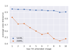
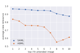
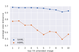
Figure 3: Predicted view relevance of top-ranked images by attention (higher is better). Supervised attention (SAMIL, ours) outperforms off-the-shelf ABMIL by wide margin across all 3 splits. The x-axis indicates a rank position of images within an echo study when sorted by attention (1 = largest $a_{k}$, 2 = second largest, etc.). The y-axis indicates the average view relevance (across studies in test set) assigned by view classifier $v(x)$ to image $x$ at rank $k$.

5.4 Ablation evaluations of attention and pretraining

	Test Set Bal. Accuracy
Method	1	2	3	average
ABMIL	58.5	60.4	61.6	60.2
ABMIL Gate Attn.	57.8	62.6	59.8	60.1
SAMIL no pretrain	72.7	71.6	73.5	72.6

Table 3: Ablation of attention strategies on TMED2. Showing balanced accuracy for AS severity (higher is better) on the test set across splits. All use  2.3 M parameters.

	Test set Bal. Accuracy
Method	1	2	3	average
SAMIL no pretrain	72.7	71.6	73.5	72.6
SAMIL w/ img-CL	71.2	67.0	75.8	71.4
SAMIL	75.4	73.8	79.4	76.2

Table 4: Ablation of pretraining strategies on TMED2. Reporting balanced accuracy for AS severity (higher is better) on the test set across splits. All use  2.3 M parameters.

The effectiveness of the supervised attention is evident in Table 4. SAMIL achieves an improvement of over 12% compared to ABMIL, the model it builds upon, even without self-supervised pretraining.

To understand what SAMIL’s built-in study-level (aka bag-level) pretraining adds, we compare to the regular approach of image-level self-supervised pretraining and without pretraining at all. Tab. 4 shows that naively using image-level pretraining does not improve AS diagnosis performance, while our proposed study-level pretraining strategy successfully delivers gains.

6 Discussion

We have developed an approach to deep multiple instance learning for diagnosing a common heart valve disease (aortic stenosis) from the dozens of images collected in a routine echocardiogram. In our evaluations on the open-access TMED-2 dataset, we find our approach reaches better classifier accuracy than several alternatives, including two recent methods dedicated to AS screening. We suspect that gains come from two sources. First, our method’s ability to use both PLAX and PSAX images, not just PLAX. Second, our method’s flexible attention that does not weight each relevant view equally. Both prior efforts on AS studied here, Filter-then-Average and Weighted Average by View Relevance, essentially treat each high-confidence PLAX or PSAX image equally in diagnosis. Instead, we emphasize that our method can learn a study-specific subset of PLAX or PSAX to attend to, based on image quality, anatomic visibility, or other factors.

Limitations in diagnostic potential.

Human experts assess AS using several additional factors not available to our method. These include patient demographics, clinical variables, and (most importantly) other imaging technologies such as doppler echocardiography as well as high-resolution cineloop videos from 2D TTE (not just lower-resolution single frame images used here). We suspect adapting our MIL architecture to these modalities would provide exciting further gains.

Limitations in evaluation.

As of this writing, TMED-2 is the only open-access dataset of echos known to us with diagnostic labels for AS or other valve disease. However, it is limited in size and in covered demographics due to drawing from just one hospital site. Further assessment is needed to understand how our proposed method generalizes, especially to populations underrepresented at the Boston-based hospital where this data was collected.

Advantages.

Our SAMIL approach is designed to perform automatic screening of an echo study without requiring a first-stage manual or automatic prefiltering to relevant view types. Even though prefiltering may sound simpler than MIL, we show our approach works better, likely due to its flexible attention mechanism. We can further leverage large unlabeled data collections for pretraining effective representations.

Our MIL approach could easily be applied to other structural heart diseases including cardiomyopathies and mitral and tricuspid disease if suitable labels were available for some studies. Additionally, multi-view image diagnostic problems are also abundant in fetal ultrasound, lung ultrasound, and head CT applications, so we expect translation of our insights to these other domains will bear fruit. Both key innovations – supervised attention to steer toward clinically-relevant views for the diagnostic task and study-level representation learning – are applicable to many other prediction tasks. Ultimately, we hope our study plays a part in transforming early screening for AS and other burdensome diseases to be more reproducible, effective, portable, and actionable.

We acknowledge financial support from the Pilot Studies Program at the Tufts Clinical and Translational Science Institute (Tufts CTSI NIH CTSA UL1TR002544). We are grateful for computing infrastructure support from the Tufts High-performance Computing cluster, partially funded by the National Science Foundation under grant OAC CC* 2018149. Author B. W. was supported in part by K23AG055667 (NIH-NIA).

[sections]

Appendix Contents

[sections]l1

Appendix A Further Results

A.1 Confusion matrix

	Split 1	Split 2	Split 3
W. Avg. by View Rel.
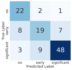
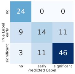
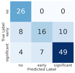
ABMIL
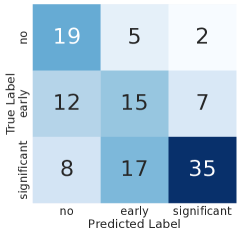
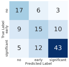
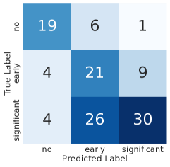
DSMIL
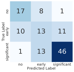
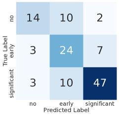
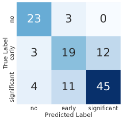
SAMIL (ours)

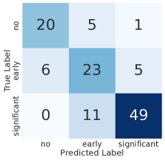
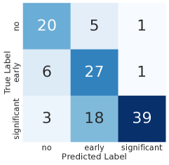
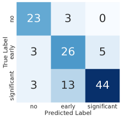
Figure A.1: Confusion matrices for the patient-level AS diagnosis classification, across three predefined train/test splits of TMED2.

A.2 ROC for AS Screening Tasks

	No vs Some AS	Early vs Significant AS	NoSignificant vs Significant AS
Split1
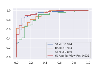
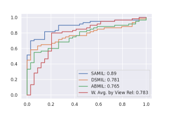
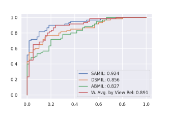
Split2
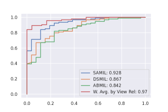
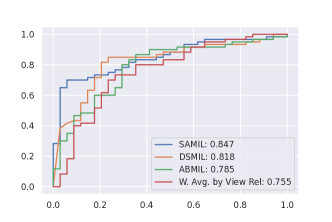
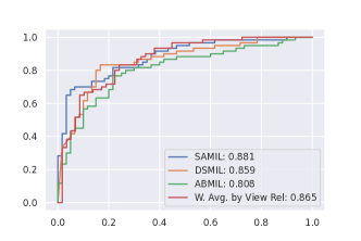
Split3

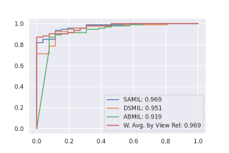
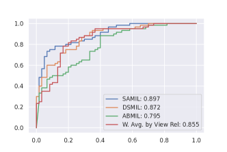
Figure A.2: Diagnosis classification receiver operator curves. Showing results across three predefined train/test splits of TMED2 and three clinically relevant screening tasks.

A.3 Attended Images by SAMIL and ABMIL

ABMIL
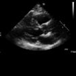
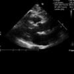
ABMIL
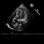
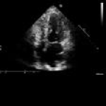
SAMIL
SAMIL

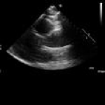
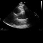
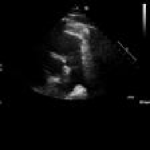
Figure A.3: Showing top attended images for the first study in the test set. The top 2 rows show the top 10 attended images by ABMIL, bottom 2 rows show the top 10 attended images by SAMIL. Red box indicates the image is not a clinically relevant view for AS diagnosis.

Appendix B Methods Supplement

B.1 Architecture

Below we report the architecture details for SAMIL. For feature extractor $f$, we use a simple stack of convolution layers as done in ABMIL (Ilse et al., 2018).

Feature Extractor $f$
Conv2d(3, 20, kernel=(5,5))
ReLU()
MaxPool2d(2, stride=2)
Conv2d(20, 50, kernel=(5,5))
ReLU()
MaxPool2d(2, stride=2)
Conv2d(50, 100, kernel=(5,5))
ReLU()
Conv2d(100, 200, kernel=(5,5))
ReLU()
MaxPool2d(2, stride=2)

Table B.1: Details of Feature Extractor $f$

We used the same feature extractor $f$ shown in B.1 for SAMIL, ABMIL, Set Transformer and DSMIL.

The feature extractor $f$ maps each of the original images into 200 feature maps with smaller size. In practice, a MLP can be use (optional) to further process the flattened feature maps (also see Fig 2). We use the same MLP [Linear(32000, 500), ReLU(), Linear(500, 250), ReLU(), Linear(250, 500), ReLU()] for both SAMIL and ABMIL. For Set Transformer, we directly flattened the extracted feature maps and feed them to the Set Transformer’s ISAB blocks. Please refer to original paper (Lee et al., 2019) for more details. For DSMIL, the extracted feature maps are flattened and projected to vectors of dimension 500 by a linear layer followed by ReLU, and then feed to its two streams. Please refer to original paper (Li et al., 2021a) for more details.

For the pooling layer $\sigma$, we use the same MLP architectures (shown in B.2) for both the supervised attention branch and flexible attention branch in SAMIL. Note that this is also the same MLP architecture to learn attention weights in ABMIL.

MLP learning attention weights
Linear(500, 128)
Tanh()
Linear(128, 1)

Table B.2: Details of MLP used to learn attention weights for SAMIL and ABMIL

For output layer $g$ both SAMIL and ABMIL use a simple linear layer (with softmax). Our experiments for DSMIL, and Set Transformer are mainly based on the official open-source code from corresponding paper. Please refer to the original papers for more details on their $\sigma$ and $g$.

B.2 View Classifier

We train a view classifier for each of the three splits independently. We train the classifiers using a recently proposed semi-supervised learning method (Huang et al., 2023) with Pi-model (Laine and Aila, 2016). We used the view labeled images in each split’s train set (as the labeled data) as well as the unlabeled set (as the unlabeled data).

The view classifiers are trained to output probabilities of three category: PLAX, PSAX and Other. The view classifiers’ performance is shown in B.3

Method	split1	split2	split3
Fix-A-Step + Pi	97.20	98.14	98.00

Table B.3: Balanced accuracy on view classification. Showing view classification on TMED2 test set’s view labeled images.

Backbone.

The view classifiers use Wide ResNet (Zagoruyko and Komodakis, 2016) as backbone, specifically, the “WRN-28-2” that has a depth 28 and width 2.

Training and Hyperparameters.

We train the view classifiers using SGD (Robbins and Monro, 1951) as optimizer. We train the classifiers for 500 epochs, and retain the checkpoint that has maximum validation accuracy on the validation set. Hyperparameters used are reported below B.4

Hyperparameter	split1	split2	split3
Labeled batch size	64	64	64
Unlabeled batch size	64	64	64
Learning rate	0.0003	0.009	0.009
Weight decay	0.05	0.0005	0.0005
Max consistency coefficient	0.3	0.3	0.3
Beta shape $\alpha$	0.5	0.5	0.5
Unlabeled loss warmup schedule	linear	linear	linear
Learning rate schedule	cosine	cosine	cosine

Table B.4: Hyperparameters used for the view classifiers in each split.

Appendix C MIL Experiment Details

C.1 Details on Filter then Avg. Approach

To apply the Filter then Avg. approach proposed on TMED2, we follow closely the steps outlined in the paper  Holste et al. (2022b, a). We first use the same view classifiers that are used for SAMIL to prefilter images in the dataset, keeping only images that are predicted as PLAX. We then use a 2D ResNet18 (He et al., 2016) to train the diagnosis classifier to classify each retained PLAX image as no AS, early AS or significant AS. In aggregation step, we average the AS predictions of all PLAX images in a study to obtain the study-level AS prediction. Note that author in  (Holste et al., 2022a) uses a 3D ResNet18 (Tran et al., 2018) since their proprietary dataset consists of 3D videos while the open access TMED2 consists of 2D images. For the same reason, we are not able to directly use their self-superivsed training strategy that are proposed for 3D videos.

C.2 Details on DeepSet

DeepSet (Zaheer et al., 2017) process each instance in the bag independently, and aggregate the processed feature embedding using simple pooling (mean or max). Fully connected layers are then used to map the aggregated feature embeddings into a bag prediction.

We perform the same hyperparameter search for DeepSet as shown below C.4. However, we won’t able to obtain any meaningful results, which suggest that problem of using multiple ultrasound images for AS diagnosis is too challenging for simple architecture like DeepSet.

C.3 Training.

Our open source code (will be released after upon acceptance) uses PyTorch  (Paszke et al., 2019). For all methods compared, we use SGD (Robbins and Monro, 1951) as optimizer. Each method is set to train for 2000 epochs, and early stop if validation performance does not increase for 200 consecutive epochs. Each training run uses one NVIDIA A100 GPU.

C.4 Hyperparameter.

We perform a grid search for each algorithm and each data split. From our preliminary experiments, we found that learning rate around 0.0005 and weight decay around 0.0001 is a good starting point.

For DSMIL, ABMIL, Set Transformer, DeepSet and Filter then Avg, we search learning rate in [0.0003, 0.0005, 0.0008, 0.001, 0.003] and weight decay in [0.00001, 0.00003, 0.0001, 0.0003, 0.001]. SAMIL involves two additional hyperparameters, a temperature scaling term $\tau_{v}$ used in eq. 4, and $\lambda_{SA}$ in eq. 8 that balance the supervised attention loss and the cross-entropy loss. For SAMIL, we search learning rate in [0.0005, 0.0008], weight decay in [0.0001, 0.001], $\tau_{v}$ in [0.1, 0.05, 0.03] and $\lambda_{SA}$ in [5, 15, 20]. Note that for ABMIL with gated attention, we did not search hyperparameters again, but directly use the corresponding best hyperparameter from its general attention version. Note that we perform same set of independent hyperparameter search for experiments on SAMIL with bag-level pretraining, image-level pretraining and without pretraining.

Final hyperparameter used are reported as follow:

SAMIL (with study-level SSL)
Hyperparameter	split1	split2	split3
Learning rate	0.0005	0.0008	0.0005
Weight decay	0.0001	0.001	0.001
Temperature T	0.1	0.1	0.05
$\lambda_{SA}$	15.0	20.0	20.0
Learning rate schedule	cosine	cosine	cosine

Table C.1: Hyperparameter settings for SAMIL across different data splits.

DSMIL
Hyperparameter	split1	split2	split3
Learning rate	0.001	0.0008	0.0008
Weight decay	0.0001	0.00003	0.00001
Learning rate schedule	cosine	cosine	cosine

Table C.2: Hyperparameter settings for DSMIL across different data splits.

ABMIL
Hyperparameter	split1	split2	split3
Learning rate	0.0008	0.0005	0.0008
Weight decay	0.0001	0.00005	0.00005
Learning rate schedule	cosine	cosine	cosine

Table C.3: Hyperparameter settings for ABMIL across different data splits.

Set Transformer
Hyperparameter	split1	split2	split3
Learning rate	0.0010	0.0008	0.0008
Weight decay	0.00003	0.0001	0.00001
Learning rate schedule	cosine	cosine	cosine

Table C.4: Hyperparameter settings for Set Transformer across different data splits.

Filter then Avg.
Hyperparameter	split1	split2	split3
Learning rate	0.003	0.001	0.003
Weight decay	0.00003	0.00001	0.00001
Learning rate schedule	cosine	cosine	cosine

Table C.5: Hyperparameter settings for Filter then Avg. across different data splits.

Appendix D Self-supervised Pretraining

Our implementation is based on the official code from MoCo (He et al., 2020; Chen et al., 2020b). For image-level contrastive learning, we set learning rate to 0.06, weight decay to 0.0005, batch size to 512, size of queue to 4096, momentum m to 0.99, softmax temperature to 0.1. For bag-level contrastive learning, we set learning rate to 0.00015 (following the linear Scaling Relu (Goyal et al., 2017), which is also recommended by MoCo’s author), weight decay to 0.0005, batch size to 1, size of queue to 4096, momentum m to 0.99, softmax temperature to 0.1. Note that we did not tune hyperparameters for the self-supervised pretraining.

We train the model using the train set as well as the unlabeled set for both image-level and bag-level contrastive learning. The model is set to train for 200 epochs, with early stopping monitored by knn protocol on the validation set. The early stopping patience is set to 20.

projection head $\psi$.

The projection head is a two-layer MLP with the structure [Linear(500, 500), ReLU(), Linear(500, 128)]. The projection head is used to project the image or bag representation to a latent space where the contrastive loss is applied. The projection head is discarded after training following the convention from  (Chen et al., 2020b, a).

Appendix E Additional Related Work

Classic approaches.

Examples of classic MIL methods includes iARP (Dietterich et al., 1997), Diverse Density (Maron and Lozano-Pérez, 1997), Citation-kNN (Wang and Zucker, 2000), MI-Kernels (Zhang and Goldman, 2001), MI/mi-SVM (Andrews et al., 2002), mi-Graph  (Zhou et al., 2009), MILBoost (Zhang et al., 2005), GPMIL (Kim and De la Torre, 2010), among others.

References

- Andrews et al. (2002) Stuart Andrews, Ioannis Tsochantaridis, and Thomas Hofmann. Support vector machines for multiple-instance learning. Advances in neural information processing systems, 15, 2002.
- Arora et al. (2019) Sanjeev Arora, Hrishikesh Khandeparkar, Mikhail Khodak, Orestis Plevrakis, and Nikunj Saunshi. A theoretical analysis of contrastive unsupervised representation learning. arXiv preprint arXiv:1902.09229, 2019.
- Ash et al. (2021) Jordan T Ash, Surbhi Goel, Akshay Krishnamurthy, and Dipendra Misra. Investigating the role of negatives in contrastive representation learning. arXiv preprint arXiv:2106.09943, 2021.
- Bachman et al. (2019) Philip Bachman, R Devon Hjelm, and William Buchwalter. Learning representations by maximizing mutual information across views. Advances in neural information processing systems, 32, 2019.
- Borowa et al. (2020) Adriana Borowa, Dawid Rymarczyk, Dorota Ochońska, Monika Brzychczy-Włoch, and Bartosz Zieliński. Classifying bacteria clones using attention-based deep multiple instance learning interpreted by persistence homology. arXiv preprint arXiv:2012.01189, 2020.
- Campanella et al. (2019) Gabriele Campanella, Matthew G Hanna, Luke Geneslaw, Allen Miraflor, Vitor Werneck Krauss Silva, Klaus J Busam, Edi Brogi, Victor E Reuter, David S Klimstra, and Thomas J Fuchs. Clinical-grade computational pathology using weakly supervised deep learning on whole slide images. Nature medicine, 25(8):1301–1309, 2019.
- Carbonneau et al. (2018) Marc-André Carbonneau, Veronika Cheplygina, Eric Granger, and Ghyslain Gagnon. Multiple instance learning: A survey of problem characteristics and applications. Pattern Recognition, 77:329–353, 2018.
- Caron et al. (2020) Mathilde Caron, Ishan Misra, Julien Mairal, Priya Goyal, Piotr Bojanowski, and Armand Joulin. Unsupervised learning of visual features by contrasting cluster assignments. Advances in neural information processing systems, 33:9912–9924, 2020.
- Chen et al. (2020a) Ting Chen, Simon Kornblith, Mohammad Norouzi, and Geoffrey Hinton. A simple framework for contrastive learning of visual representations. In International conference on machine learning, pages 1597–1607. PMLR, 2020a.
- Chen and He (2021) Xinlei Chen and Kaiming He. Exploring simple siamese representation learning. In Proceedings of the IEEE/CVF conference on computer vision and pattern recognition, pages 15750–15758, 2021.
- Chen et al. (2020b) Xinlei Chen, Haoqi Fan, Ross Girshick, and Kaiming He. Improved baselines with momentum contrastive learning. arXiv preprint arXiv:2003.04297, 2020b.
- Chikontwe et al. (2020) Philip Chikontwe, Meejeong Kim, Soo Jeong Nam, Heounjeong Go, and Sang Hyun Park. Multiple instance learning with center embeddings for histopathology classification. In Medical Image Computing and Computer Assisted Intervention–MICCAI 2020: 23rd International Conference, Lima, Peru, October 4–8, 2020, Proceedings, Part V 23, pages 519–528. Springer, 2020.
- Chuang et al. (2020) Ching-Yao Chuang, Joshua Robinson, Yen-Chen Lin, Antonio Torralba, and Stefanie Jegelka. Debiased contrastive learning. Advances in neural information processing systems, 33:8765–8775, 2020.
- Cohen-Shelly et al. (2021) Michal Cohen-Shelly, Zachi I Attia, Paul A Friedman, Saki Ito, Benjamin A Essayagh, Wei-Yin Ko, Dennis H Murphree, Hector I Michelena, Maurice Enriquez-Sarano, Rickey E Carter, et al. Electrocardiogram screening for aortic valve stenosis using artificial intelligence. European heart journal, 42(30), 2021.
- Cosatto et al. (2013) Eric Cosatto, Pierre-Francois Laquerre, Christopher Malon, Hans-Peter Graf, Akira Saito, Tomoharu Kiyuna, Atsushi Marugame, and Ken’ichi Kamijo. Automated gastric cancer diagnosis on h&e-stained sections; ltraining a classifier on a large scale with multiple instance machine learning. In Medical Imaging 2013: Digital Pathology, volume 8676, pages 51–59. SPIE, 2013.
- Dai et al. (2023) Wangzhi Dai, Hamed Nazzari, Mayooran Namasivayam, Judy Hung, and Collin M Stultz. Identifying aortic stenosis with a single parasternal long-axis video using deep learning. Journal of the American Society of Echocardiography, 36(1), 2023.
- Dehaene et al. (2020) Olivier Dehaene, Axel Camara, Olivier Moindrot, Axel de Lavergne, and Pierre Courtiol. Self-supervision closes the gap between weak and strong supervision in histology. arXiv preprint arXiv:2012.03583, 2020.
- Dietterich et al. (1997) Thomas G Dietterich, Richard H Lathrop, and Tomás Lozano-Pérez. Solving the multiple instance problem with axis-parallel rectangles. Artificial intelligence, 89(1-2):31–71, 1997.
- Ding et al. (2012) Jianrui Ding, Heng-Da Cheng, Jianhua Huang, Jiafeng Liu, and Yingtao Zhang. Breast ultrasound image classification based on multiple-instance learning. Journal of digital imaging, 25:620–627, 2012.
- Dwibedi et al. (2021) Debidatta Dwibedi, Yusuf Aytar, Jonathan Tompson, Pierre Sermanet, and Andrew Zisserman. With a little help from my friends: Nearest-neighbor contrastive learning of visual representations. In Proceedings of the IEEE/CVF International Conference on Computer Vision, pages 9588–9597, 2021.
- Elias et al. (2022) Pierre Elias, Timothy J Poterucha, Vijay Rajaram, Luca Matos Moller, Victor Rodriguez, Shreyas Bhave, Rebecca T Hahn, Geoffrey Tison, Sean A Abreau, Joshua Barrios, et al. Deep learning electrocardiographic analysis for detection of left-sided valvular heart disease. Journal of the American College of Cardiology, 80(6):613–626, 2022.
- Gardezi et al. (2018) Syed KM Gardezi, Saul G Myerson, John Chambers, Sean Coffey, Joanna d’Arcy, FD Richard Hobbs, Jonathan Holt, Andrew Kennedy, Margaret Loudon, Anne Prendergast, et al. Cardiac auscultation poorly predicts the presence of valvular heart disease in asymptomatic primary care patients. Heart, 104(22):1832–1835, 2018.
- Gidaris et al. (2018) Spyros Gidaris, Praveer Singh, and Nikos Komodakis. Unsupervised representation learning by predicting image rotations. arXiv preprint arXiv:1803.07728, 2018.
- Goyal et al. (2017) Priya Goyal, Piotr Dollár, Ross Girshick, Pieter Noordhuis, Lukasz Wesolowski, Aapo Kyrola, Andrew Tulloch, Yangqing Jia, and Kaiming He. Accurate, large minibatch sgd: Training imagenet in 1 hour. arXiv preprint arXiv:1706.02677, 2017.
- Grill et al. (2020) Jean-Bastien Grill, Florian Strub, Florent Altché, Corentin Tallec, Pierre Richemond, Elena Buchatskaya, Carl Doersch, Bernardo Avila Pires, Zhaohan Guo, Mohammad Gheshlaghi Azar, et al. Bootstrap your own latent-a new approach to self-supervised learning. Advances in neural information processing systems, 33:21271–21284, 2020.
- He et al. (2016) Kaiming He, Xiangyu Zhang, Shaoqing Ren, and Jian Sun. Deep residual learning for image recognition. In Proceedings of the IEEE conference on computer vision and pattern recognition, pages 770–778, 2016.
- He et al. (2020) Kaiming He, Haoqi Fan, Yuxin Wu, Saining Xie, and Ross Girshick. Momentum contrast for unsupervised visual representation learning. In Proceedings of the IEEE/CVF conference on computer vision and pattern recognition, pages 9729–9738, 2020.
- Hinton et al. (2015) Geoffrey Hinton, Oriol Vinyals, and Jeff Dean. Distilling the knowledge in a neural network. arXiv preprint arXiv:1503.02531, 2015.
- Holste et al. (2022a) Gregory Holste, Evangelos K Oikonomou, Bobak Mortazavi, Zhangyang Wang, and Rohan Khera. Self-supervised learning of echocardiogram videos enables data-efficient clinical diagnosis. arXiv preprint arXiv:2207.11581, 2022a.
- Holste et al. (2022b) Gregory Holste, Evangelos K Oikonomou, Bobak J Mortazavi, Andreas Coppi, Kamil F Faridi, Edward J Miller, John K Forrest, Robert L McNamara, Lucila Ohno-Machado, Neal Yuan, et al. Automated severe aortic stenosis detection on single-view echocardiography: A multi-center deep learning study. medRxiv, 2022b.
- Holzinger et al. (2017) Andreas Holzinger, Chris Biemann, Constantinos S Pattichis, and Douglas B Kell. What do we need to build explainable ai systems for the medical domain? arXiv preprint arXiv:1712.09923, 2017.
- Hou et al. (2016) Le Hou, Dimitris Samaras, Tahsin M Kurc, Yi Gao, James E Davis, and Joel H Saltz. Patch-based convolutional neural network for whole slide tissue image classification. In Proceedings of the IEEE conference on computer vision and pattern recognition, pages 2424–2433, 2016.
- Huang et al. (2021) Zhe Huang, Gary Long, Benjamin Wessler, and Michael C Hughes. A new semi-supervised learning benchmark for classifying view and diagnosing aortic stenosis from echocardiograms. In Machine Learning for Healthcare Conference, 2021. URL https://proceedings.mlr.press/v149/huang21a.html.
- Huang et al. (2022) Zhe Huang, Gary Long, Benjamin S Wessler, and Michael C Hughes. TMED 2: A dataset for semi-supervised classification of echocardiograms. In DataPerf: Benchmarking Data for Data-Centric AI Workshop at ICML, 2022.
- Huang et al. (2023) Zhe Huang, Mary-Joy Sidhom, Benjamin S Wessler, and Michael C Hughes. Fix-a-step: Semi-supervised learning from uncurated unlabeled data. In Artificial Intelligence and Statistics (AISTATS), 2023. URL https://proceedings.mlr.press/v206/huang23c.html.
- Ilse et al. (2018) Maximilian Ilse, Jakub Tomczak, and Max Welling. Attention-based deep multiple instance learning. In International conference on machine learning, pages 2127–2136. PMLR, 2018.
- Kandemir and Hamprecht (2015) Melih Kandemir and Fred A Hamprecht. Computer-aided diagnosis from weak supervision: A benchmarking study. Computerized medical imaging and graphics, 42:44–50, 2015.
- Khosla et al. (2020) Prannay Khosla, Piotr Teterwak, Chen Wang, Aaron Sarna, Yonglong Tian, Phillip Isola, Aaron Maschinot, Ce Liu, and Dilip Krishnan. Supervised contrastive learning. Advances in neural information processing systems, 33:18661–18673, 2020.
- Kim and De la Torre (2010) Minyoung Kim and Fernando De la Torre. Gaussian processes multiple instance learning. In ICML, pages 535–542. Citeseer, 2010.
- Krishna et al. (2023) Hema Krishna, Kevin Desai, Brody Slostad, Siddharth Bhayani, Joshua H Arnold, Wouter Ouwerkerk, Yoran Hummel, Carolyn SP Lam, Justin Ezekowitz, Matthew Frost, et al. Fully automated artificial intelligence assessment of aortic stenosis by echocardiography. Journal of the American Society of Echocardiography, 2023.
- Laine and Aila (2016) Samuli Laine and Timo Aila. Temporal ensembling for semi-supervised learning. arXiv preprint arXiv:1610.02242, 2016.
- Lee et al. (2019) Juho Lee, Yoonho Lee, Jungtaek Kim, Adam Kosiorek, Seungjin Choi, and Yee Whye Teh. Set transformer: A framework for attention-based permutation-invariant neural networks. In International conference on machine learning, pages 3744–3753. PMLR, 2019.
- Li et al. (2021a) Bin Li, Yin Li, and Kevin W Eliceiri. Dual-stream multiple instance learning network for whole slide image classification with self-supervised contrastive learning. In Proceedings of the IEEE/CVF conference on computer vision and pattern recognition (CVPR), 2021a.
- Li et al. (2021b) Junnan Li, Caiming Xiong, and Steven CH Hoi. Comatch: Semi-supervised learning with contrastive graph regularization. In Proceedings of the IEEE/CVF international conference on computer vision, pages 9475–9484, 2021b.
- Li et al. (2021c) Xirong Li, Wencui Wan, Yang Zhou, Jianchun Zhao, Qijie Wei, Junbo Rong, Pengyi Zhou, Limin Xu, Lijuan Lang, Yuying Liu, et al. Deep multiple instance learning with spatial attention for rop case classification, instance selection and abnormality localization. In 2020 25th International Conference on Pattern Recognition (ICPR), pages 7293–7298. IEEE, 2021c.
- Li et al. (2021d) Xirong Li, Yang Zhou, Jie Wang, Hailan Lin, Jianchun Zhao, Dayong Ding, Weihong Yu, and Youxin Chen. Multi-modal multi-instance learning for retinal disease recognition. In Proceedings of the 29th ACM International Conference on Multimedia, pages 2474–2482, 2021d.
- Liu et al. (2022) Kangning Liu, Weicheng Zhu, Yiqiu Shen, Sheng Liu, Narges Razavian, Krzysztof J Geras, and Carlos Fernandez-Granda. Multiple instance learning via iterative self-paced supervised contrastive learning. arXiv preprint arXiv:2210.09452, 2022.
- Liu et al. (2017) Yun Liu, Krishna Gadepalli, Mohammad Norouzi, George E Dahl, Timo Kohlberger, Aleksey Boyko, Subhashini Venugopalan, Aleksei Timofeev, Philip Q Nelson, Greg S Corrado, et al. Detecting cancer metastases on gigapixel pathology images. arXiv preprint arXiv:1703.02442, 2017.
- Long and Wessler (2018) Gary Long and Benjamin S Wessler. Identification of echocardiographic imaging view using deep learning. Circulation: Cardiovascular Quality and Outcomes, 11(suppl_1):A276–A276, 2018.
- Lu et al. (2019) Ming Y Lu, Richard J Chen, Jingwen Wang, Debora Dillon, and Faisal Mahmood. Semi-supervised histology classification using deep multiple instance learning and contrastive predictive coding. arXiv preprint arXiv:1910.10825, 2019.
- Lundberg and Lee (2017) Scott M Lundberg and Su-In Lee. A unified approach to interpreting model predictions. Advances in neural information processing systems, 30, 2017.
- Madani et al. (2018) Ali Madani, Ramy Arnaout, Mohammad Mofrad, and Rima Arnaout. Fast and accurate view classification of echocardiograms using deep learning. NPJ digital medicine, 1(1):6, 2018.
- Maron and Lozano-Pérez (1997) Oded Maron and Tomás Lozano-Pérez. A framework for multiple-instance learning. Advances in neural information processing systems, 10, 1997.
- Mitchell et al. (2019) Carol Mitchell, Peter S Rahko, Lori A Blauwet, Barry Canaday, Joshua A Finstuen, Michael C Foster, Kenneth Horton, Kofo O Ogunyankin, Richard A Palma, and Eric J Velazquez. Guidelines for performing a comprehensive transthoracic echocardiographic examination in adults: recommendations from the american society of echocardiography. Journal of the American Society of Echocardiography, 32(1):1–64, 2019.
- Noroozi and Favaro (2016) Mehdi Noroozi and Paolo Favaro. Unsupervised learning of visual representations by solving jigsaw puzzles. In Computer Vision–ECCV 2016: 14th European Conference, Amsterdam, The Netherlands, October 11-14, 2016, Proceedings, Part VI, pages 69–84. Springer, 2016.
- Oord et al. (2018) Aaron van den Oord, Yazhe Li, and Oriol Vinyals. Representation learning with contrastive predictive coding. arXiv preprint arXiv:1807.03748, 2018.
- Paszke et al. (2019) Adam Paszke, Sam Gross, Francisco Massa, Adam Lerer, James Bradbury, Gregory Chanan, Trevor Killeen, Zeming Lin, Natalia Gimelshein, Luca Antiga, et al. Pytorch: An imperative style, high-performance deep learning library. Advances in neural information processing systems, 32, 2019.
- Quellec et al. (2012) Gwénolé Quellec, Mathieu Lamard, Michael D Abràmoff, Etienne Decencière, Bruno Lay, Ali Erginay, Béatrice Cochener, and Guy Cazuguel. A multiple-instance learning framework for diabetic retinopathy screening. Medical image analysis, 16(6):1228–1240, 2012.
- Quellec et al. (2017) Gwenolé Quellec, Guy Cazuguel, Béatrice Cochener, and Mathieu Lamard. Multiple-instance learning for medical image and video analysis. IEEE reviews in biomedical engineering, 10:213–234, 2017.
- Robbins and Monro (1951) Herbert Robbins and Sutton Monro. A stochastic approximation method. The Annals of Mathematical Statistics, 22(3):400–407, 1951.
- Rymarczyk et al. (2023) Dawid Rymarczyk, Adam Pardyl, Jarosław Kraus, Aneta Kaczyńska, Marek Skomorowski, and Bartosz Zieliński. Protomil: Multiple instance learning with prototypical parts for whole-slide image classification. In Machine Learning and Knowledge Discovery in Databases: European Conference, ECML PKDD 2022, Grenoble, France, September 19–23, 2022, Proceedings, Part I, pages 421–436. Springer, 2023.
- Saillard et al. (2021) Charlie Saillard, Olivier Dehaene, Tanguy Marchand, Olivier Moindrot, Aurélie Kamoun, Benoit Schmauch, and Simon Jegou. Self supervised learning improves dmmr/msi detection from histology slides across multiple cancers. arXiv preprint arXiv:2109.05819, 2021.
- Shao et al. (2021) Zhuchen Shao, Hao Bian, Yang Chen, Yifeng Wang, Jian Zhang, Xiangyang Ji, et al. Transmil: Transformer based correlated multiple instance learning for whole slide image classification. Advances in neural information processing systems, 34:2136–2147, 2021.
- Sharma et al. (2021) Yash Sharma, Aman Shrivastava, Lubaina Ehsan, Christopher A Moskaluk, Sana Syed, and Donald Brown. Cluster-to-conquer: A framework for end-to-end multi-instance learning for whole slide image classification. In Medical Imaging with Deep Learning, pages 682–698. PMLR, 2021.
- Tonekaboni et al. (2019) Sana Tonekaboni, Shalmali Joshi, Melissa D McCradden, and Anna Goldenberg. What clinicians want: contextualizing explainable machine learning for clinical end use. In Machine learning for healthcare conference, pages 359–380. PMLR, 2019.
- Tran et al. (2018) Du Tran, Heng Wang, Lorenzo Torresani, Jamie Ray, Yann LeCun, and Manohar Paluri. A closer look at spatiotemporal convolutions for action recognition. In Proceedings of the IEEE conference on Computer Vision and Pattern Recognition, pages 6450–6459, 2018.
- Vaswani et al. (2017) Ashish Vaswani, Noam Shazeer, Niki Parmar, Jakob Uszkoreit, Llion Jones, Aidan N Gomez, Łukasz Kaiser, and Illia Polosukhin. Attention is all you need. Advances in neural information processing systems, 30, 2017.
- Wang and Zucker (2000) Jun Wang and Jean-Daniel Zucker. Solving multiple-instance problem: A lazy learning approach. In International Conference on Machine Learnign (ICML), 2000.
- Wang et al. (2018) Xinggang Wang, Yongluan Yan, Peng Tang, Xiang Bai, and Wenyu Liu. Revisiting multiple instance neural networks. Pattern Recognition, 74:15–24, 2018.
- Wessler et al. (2023) Benjamin S Wessler, Zhe Huang, Gary M Long Jr, Stefano Pacifici, Nishant Prashar, Samuel Karmiy, Roman A Sandler, Joseph Z Sokol, Daniel B Sokol, Monica M Dehn, et al. Automated detection of aortic stenosis using machine learning. Journal of the American Society of Echocardiography, 2023.
- Wu et al. (2018) Zhirong Wu, Yuanjun Xiong, Stella X Yu, and Dahua Lin. Unsupervised feature learning via non-parametric instance discrimination. In Proceedings of the IEEE conference on computer vision and pattern recognition (CVPR), 2018.
- Xu et al. (2014) Yan Xu, Jun-Yan Zhu, I Eric, Chao Chang, Maode Lai, and Zhuowen Tu. Weakly supervised histopathology cancer image segmentation and classification. Medical image analysis, 18(3):591–604, 2014.
- Yadgir et al. (2020) Simon Yadgir, Catherine Owens Johnson, Victor Aboyans, Oladimeji M Adebayo, Rufus Adesoji Adedoyin, Mohsen Afarideh, Fares Alahdab, Alaa Alashi, Vahid Alipour, Jalal Arabloo, et al. Global, regional, and national burden of calcific aortic valve and degenerative mitral valve diseases, 1990–2017. Circulation, 141(21):1670–1680, 2020.
- Yang et al. (2020) Chenxi Yang, Banish D. Ojha, Nicole D. Aranoff, Philip Green, and Negar Tavassolian. Classification of aortic stenosis using conventional machine learning and deep learning methods based on multi-dimensional cardio-mechanical signals. Scientific Reports, 10(1), 2020.
- Ye et al. (2019) Mang Ye, Xu Zhang, Pong C Yuen, and Shih-Fu Chang. Unsupervised embedding learning via invariant and spreading instance feature. In Proceedings of the IEEE/CVF Conference on Computer Vision and Pattern Recognition, pages 6210–6219, 2019.
- Zagoruyko and Komodakis (2016) Sergey Zagoruyko and Nikos Komodakis. Wide residual networks. arXiv preprint arXiv:1605.07146, 2016.
- Zaheer et al. (2017) Manzil Zaheer, Satwik Kottur, Siamak Ravanbakhsh, Barnabas Poczos, Russ R Salakhutdinov, and Alexander J Smola. Deep sets. Advances in neural information processing systems, 30, 2017.
- Zhang et al. (2005) Cha Zhang, John Platt, and Paul Viola. Multiple instance boosting for object detection. Advances in neural information processing systems, 18, 2005.
- Zhang et al. (2018) Jeffrey Zhang, Sravani Gajjala, Pulkit Agrawal, Geoffrey H Tison, Laura A Hallock, Lauren Beussink-Nelson, Mats H Lassen, Eugene Fan, Mandar A Aras, ChaRandle Jordan, et al. Fully automated echocardiogram interpretation in clinical practice: feasibility and diagnostic accuracy. Circulation, 138(16):1623–1635, 2018.
- Zhang and Goldman (2001) Qi Zhang and Sally Goldman. Em-dd: An improved multiple-instance learning technique. Advances in neural information processing systems, 14, 2001.
- Zhao et al. (2013) Zhendong Zhao, Gang Fu, Sheng Liu, Khaled M Elokely, Robert J Doerksen, Yixin Chen, and Dawn E Wilkins. Drug activity prediction using multiple-instance learning via joint instance and feature selection. BMC bioinformatics, 14(S16), 2013. URL https://doi.org/10.1186/1471-2105-14-S14-S16.
- Zheng et al. (2021) Mingkai Zheng, Fei Wang, Shan You, Chen Qian, Changshui Zhang, Xiaogang Wang, and Chang Xu. Weakly supervised contrastive learning. In Proceedings of the IEEE/CVF International Conference on Computer Vision, pages 10042–10051, 2021.
- Zhou (2004) Zhi-Hua Zhou. Multi-instance learning: A survey. Department of Computer Science & Technology, Nanjing University, Tech. Rep, 1, 2004.
- Zhou et al. (2009) Zhi-Hua Zhou, Yu-Yin Sun, and Yu-Feng Li. Multi-instance learning by treating instances as non-iid samples. In Proceedings of the 26th annual international conference on machine learning, pages 1249–1256, 2009.