Arbitrarily accurate, nonparametric coarse graining with Markov renewal processes and the Mori-Zwanzig formulation

Abstract

Stochastic dynamics, such as molecular dynamics, are important in many scientific applications. However, summarizing and analyzing the results of such simulations is often challenging, due to the high dimension in which simulations are carried out, and consequently to the very large amount of data that is typically generated. Coarse graining is a popular technique for addressing this problem by providing compact and expressive representations. Coarse graining, however, potentially comes at the cost of accuracy, as dynamical information is in general lost when projecting the problem in a lower dimensional space. This article shows how to eliminate coarse-graining error using two key ideas. First, we represent coarse-grained dynamics as a Markov renewal process. Second, we outline a data-driven, non-parametric Mori-Zwanzig approach for computing jump times of the renewal process. Numerical tests on a small protein illustrate the method.

I Introduction

Stochastic dynamics play a critical role in the study of complex systems across various scientific domains. Molecular dynamics (MD), for instance, simulate the motion of collections of atoms over time. MD simulations have found applications in materials science, chemistry, biology, and physics Karplus and Petsko (1990); Karplus and McCammon (2002); Hansson et al. (2002); Durrant and McCammon (2011); Hospital et al. (2015); Hollingsworth and Dror (2018).Analyzing the immense volume of data generated, and navigating the high-dimensional space in which these simulations operate, creates significant challenges. Indeed, a single snapshot of an MD trajectory resides in a continuous 3$N_{\mathrm{atom}}$-dimensional space, with $N_{\mathrm{atom}}$ ranging from hundreds to billions. This makes model reduction highly desirable. Effective model reduction not only enhances interpretability, but also allows for upscaling results to inform higher-fidelity models.

Yet another challenge comes from metastability Chong et al. (2017) where stochastic trajectories are confined to small regions of space for long times, punctuated by rare but fast transitions between regions. Metastability is typical in MD, where such regions might represent folded and unfolded states of a protein. In addition to MD, metastable stochastic dynamics arise in climate models Weare (2009); Webber et al. (2019); Finkel et al. (2023a, b), granular flows Seiden and Thomas (2011), neural evolution Fingelkurts and Fingelkurts (2004); Haldeman and Beggs (2005); Hellyer et al. (2015); Córdova-Palomera et al. (2017); Naik et al. (2017); Cavanna et al. (2018), hydrodynamics Pomeau (1986), and power networks Matthews et al. (2018), in addition to various ordinary differential equations models Duncan and Dunwell (2002); Sun and Ward (1999); Estep (1994); Groisman et al. (2018).

Coarse-graining is a common approach for handling high dimensionality or metastability. It is based on dividing the original high-dimensional space of microstates into a discrete set of macrostates. Usually, the dynamics on the macrostates is modeled as a Continuous Time Markov Chain (CTMC) Norris (1998) or a discrete time Markov chain (DTMC) Norris (1998); Durrett and Durrett (1999). In MD, such CTMC models are called chemical reaction networks or Kinetic Monte Carlo models Angeli (2009); Voter (2007), and the DTMCs are called Markov State Models Chodera and Noé (2014). These Markovian models offer advantages like formal simplicity, compact representation, and ease of use with ready-made algorithms like BKL Bortz et al. (1975) or Gillespie Gillespie (1977) for simulation.

The Markov assumption underlying CTMC and DTMC models is significantly flawed if macrostates are not carefully chosen Husic and Pande (2018), if temperatures are not sufficiently low Di Gesù et al. (2016), or if time scales are not long enough. Even with careful choices of all these parameters, some degree of departure from exact Markovian behavior remain in general Ross (1995); Brémaud (2001); Lelièvre (2015, 2020).

Meanwhile, recent findings show the Markov assumption can be weakened, with an arbitrarily accurate representation achievable using Markov Renewal Processes Cinlar (1975) (MRPs) by simply adjusting a scalar parameter Agarwal et al. (2020). This scalar parameter, called $\tau$ below, is a decorrelation time chosen to allow the underlying dynamics to periodically reach local equilibrium in the macrostates, inheriting the Markov property at each such time. MRPs differ from Markov processes in only having the Markov property at certain times (called jump times). Despite having formal simplicity, a complete MRP parametrization for $N$ macrostates would require $N^{2}$ scalars and $N^{2}$ functions of time. Accurately representing these functions from limited, short-time length data poses a challenge Agarwal et al. (2020). This article proposes a new technique, rooted in first principles, to efficiently model this MRP with a few $N\times N$ matrices.

I.1 Contributions

Below, we propose a compact, data-driven parametrization for the MRP model described in Agarwal et al. (2020). Our methods, rooted in Mori-Zwanzig theory, are simple and data-driven, and our contributions are practical and theoretical.

On the practical side, we propose a compact, mathematically principled representation of the MRP derived from Mori-Zwanzig theory. In our formulation, the MRP is represented by, and can be generated from, a (small) number of memory kernels. These memory kernels are $N\times N$ matrices, where $N$ is the number of macrostates. We propose a new method to obtain the kernels by solving a certain linear system comprised of correlation matrices. Efficient, scalable solvers designed for positive semidefinite systems can then be used to obtain the kernels. (E.g., RPCholesky Chen et al. (2022); Díaz et al. (2023) uses randomized low-rank approximation.) Numerical results on alanine dipeptide, a small protein, illustrate the promise of the method.

On the theoretical side, we show that these methods become exact as the number of memory kernels and the decorrelation time grow. This demonstration takes the following steps. To start, we give the first proof that coarse-grained dynamics described in Agarwal et al. (2020) in fact converges to a MRP (Theorem A.1). Then, we represent the transition probabilities of the MRP in terms of memory kernels using the discrete Mori Zwanzig equation (3). And finally, we prove that equation (3) is exact (Theorem D.2). This equation first appeared in Cao et al. (2020) in a different setting (without the decorrelation). There, it was derived as an approximation of a continuous time Mori-Zwanzig equation. We give the first full derivation of (3) that shows it is exact for any choice of dynamical lag (we use lag $\tau$ in our setup). As $\tau$ can be significantly longer than the time step of the underlying dynamical integrator, exactness at the discrete time level is important.

In addition, we provide exact expressions for the memory kernels in terms of an orthogonal dynamics (Appendix D). While these expressions cannot directly be put to practical use, they help lend explainability to the kernels, and could potentially be used to quantify their decay in time. Our novel data-driven method for actually computing the memory kernels, based on the linear solve (5), can also be explained in terms of inter-macrostate correlations.

Finally, we show that our Mori-Zwanzig equation is optimal, in the sense that the representation is compact when the MRP representation is almost fully Markovian. We actually prove an ideal case of this, showing that all but one of the memory kernels vanishes in the case where the MRP representation is in fact Markovian.

This article is organized as follows. We summarize our notation in Table 1. In Section II, we review how we discretize the underlying dynamics, followingAgarwal et al. (2020). In Section III, we introduce the Mori-Zwanzig equation and explain how we use it to estimate memory kernels nonparametrically from short time simulations. We also show how the memory kernels can be used to infer longer time information. In Section IV, we give an outline of our proof that the discretized dynamics converges to a MRP (the proof is in Appendix A). In Section V, we illustrate our method on alanine dipeptide. We show that we can reduce errors arising from ordinary spatial discretization, recovering accurate dynamics with a relatively small number of memory kernels. All proofs, including the derivation of the Mori-Zwanzig equation and the proof of convergence to a MRP, are in the Appendix.

Table 1: Definitions of symbols used in this work.

Symbol	Definition
$X(t)$	underlying Markov chain on microstates
$x$, $y$, $z$	microstates
$I$, $J$, $L$	macrostates
$N$	number of macrostates
$\tau$	macroscopic time step
$R(t)$	macroscopic jump process
$r$, $s$, $t$	times (multiples of $\tau$, when associated with $R(t)$)
$s_{-}$, $t_{-}$	preceding times: $s_{-}=s-\tau$, $t_{-}=t-\tau$
$\tau_{I}$	decorrelation time in macrostate $I$
$\eta_{I}$	QSD in macrostate $I$
$\mathcal{T}(s,t)$	transition probability matrix
$\mathcal{T}(t)$	transition matrix of renewal process
$\mathcal{P}(t)$	jump probability matrix
$\mathcal{K}(t)$	memory kernel matrix
$C(t)$	consecutive time in current macrostate
$P$, $Q$	projector and complementary projector
$\chi_{I}$	characteristic function of macrostate $I$
$n,m$	nonnegative integers

II Markov chains and Markov renewal process

Throughout, $X(t)$ is an underlying Markov process evolving in a space of microstates. This process can be discrete or continuous in both time and space. We consider a division of microstates into finitely many macrostates $I$, $J$, etc.

Our work focuses on a discrete time jump process $R(t)$ on these macrostates, with time step $\tau$, defined from the underlying process and a set of decorrelation times, written $\tau_{I}$, $\tau_{J}$, etc. The jumps occur when $X(t)$ spends consecutive time $\tau_{J}$ in some macrostate $J$. Specifically, $R(t)$ jumps from $I$ to $J$ at time $t$ if $X(t-c)$ is in macrostate $J$ for $0\leq c\leq\tau_{J}$. Jumps only occur among distinct states ($J\neq I$) and at multiples of the time step ($t=n\tau$ for integer $n$). See Figure 1 for an illustration.

To describe the evolution of $R(t)$, we define $\mathcal{T}_{IJ}(s,t)$ as the probability for $R(t)$ to be in $J$ at time $s+t$, assuming there was a jump into $I$ at time $s$. That is,

$$\mathcal{T}_{IJ}(s,t)={\mathbb{P}}(R(s+t)=J|R(s_{-})\neq I,\,R(s)=I),$$ (1)

where we use the shorthand $s_{-}=s-\tau$.

The introduction of decorrelation times allows the underlying Markov process to reach a local equilibrium within each macrostate. Conceptually, when $\tau_{J}$ is large enough, $X(t)$ loses memory of how it entered $J$ by the time that $R(t)$ jumps into macrostate $J$. This makes $R(t)$ into a MRP, which means it has the Markov property at jump times Agarwal et al. (2020). Note that $R(t)$ does not retain information about what occurs on timescales shorter than the decorrelation times and $\tau$. This is a modeling assumption that may lead to the loss of relevant dynamical information if important transition events occur on such timescales. On the other hand, information loss will be minimal when the typical residence time in a macrostate is much longer than both $\tau$ and the decorrelation time.

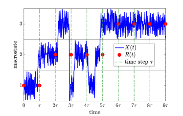
Figure 1: Illustration of $X(t)$ and $R(t)$, with three macrostates labeled $1,2,3$, when the decorrelation times are $\tau_{1}=\tau_{2}=\tau_{3}=\tau$. Solid horizontal lines divide the macrostates. For illustrative purposes, we show an example where $X(t)$ makes several transitions that are not recorded by $R(t)$, due to a failure to decorrelate in macrostates.

Assuming that $R(t)$ is in fact a MRP, we can write $\mathcal{T}(s,t)=\mathcal{T}(t)$, where $\mathcal{T}(t)$ is a standard transition matrix for each $t$. These transition matrices together satisfy a renewal equation defined by a jump probability matrix $\mathcal{P}(t)$, where $\mathcal{P}_{IJ}(t)$ is the probability for $R(t)$ to jump from $I$ to $J$ in time $t$:

$$\mathcal{P}_{IJ}(t)={\mathbb{P}}(R(s+t)=J|R(s_{-})\neq I,\,R(s^{\prime})=I,\,s\leq s^{\prime}<s+t).$$

The renewal equation is Cinlar (1975)

$$\mathcal{T}(t)=\sum_{0<s\leq t}\mathcal{P}(s)\mathcal{T}(t-s)+\mathcal{F}(t),$$ (2)

where $\mathcal{F}_{IJ}(t)=\delta_{I=J}\sum_{L}\sum_{s>t}\mathcal{P}_{IL}(s)$. Here, $\delta_{I=J}=1$ if $I=J$, and $\delta_{I=J}=0$ otherwise. The time arguments here are multiples of $\tau$, and we continue with this convention for other equations associated with $R(t)$ below.

The Markov renewal framework of (2) is exact in the limit of large decorrelation times (Theorem A.1). Below, we outline how to estimate $\mathcal{T}(t)$ in a principled, parameter-free way using Mori-Zwanzig theory. Once $\mathcal{T}(t)$ is estimated, equation (2) can be used to compute the jump time distribution $\mathcal{P}(t)$. This provides a principled way to describe – and simulate – the process $R(t)$, which exactly reflects the macroscopic behavior of $X(t)$.

Our setup above allows for situations where the decorrelation times are state-dependent: there is a (potentially different) decorrelation time $\tau_{I}$ for each macrostate $I$. For simplicity, in the numerical examples and ensuing discussion in Section V, we take all the decorrelation times to be the same and equal to $\tau$, i.e., $\tau_{I}=\tau$ for each $I$.

III Nonparametric estimation of transition probabilities

Using Mori-Zwanzig theory,

$$\mathcal{T}(t)=\sum_{0<s\leq t}\mathcal{K}(s)\mathcal{T}(t-s),$$ (3)

where $\mathcal{K}(s)$ are memory kernels that can be estimated from data, as we describe below. Equation (3) was derived as an approximation of a continuous-time Mori Zwanzig equation in Cao et al. (2020), while different discrete time Mori-Zwanzig equations have been described in Darve et al. (2009); Lin et al. (2021). We will give a short proof of exactness of (3) in Appendix D (Theorem D.2), and provide more details on the memory kernel structure there.

Equations (2) and (3) appear superficially similar but are quite different. While $\mathcal{P}(s)$ defines jump probabilities of the MRP, $\mathcal{K}(s)$ involves quantities associated to a so-called orthogonal dynamics. Roughly speaking, this dynamics describes situations where $X(t)$ transitions between macrostates without decorrelating in them. We arrived at (3) by choosing a Mori-Zwanzig projector that leads to very compact representations (i.e., fast time decay of memory kernels) when $R(t)$ is nearly Markovian. Indeed, in Appendix D, we show that if $R(t)$ is actually Markovian, only one memory kernel is nonzero, $\mathcal{K}(s)=0$ for $s>\tau$. Meanwhile, if $R(t)$ is Markovian, then $\mathcal{P}(s)$ is geometric in $s$ with rates in inverse proportion to the mean jump times between macrostates (resulting in slow decay of $\mathcal{P}(s)$ for large mean jump times).

While equation (3) could be used to solve for the memory kernels directly given enough sampling Cao et al. (2020), we find that the following setup is superior in practice. In order to nonparametrically estimate $\mathcal{K}(t)$, we introduce a loss function

$${\mathcal{L}}(\mathcal{K})=\sum_{t\leq t_{max}}\left\|\mathcal{T}(t)-\sum_{0<s\leq\min\{t,t_{mem}\}}\mathcal{K}(s)\mathcal{T}(t-s)\right\|^{2},$$ (4)

where $t_{mem}$ is a cutoff time for the memory matrices, $t_{max}$ is a cutoff time for the transition matrices, and $\|\cdot\|$ represents the Frobenius norm.

By setting the gradient of the loss function equal to zero, we get the following symmetric positive semidefinite linear system that can be solved for the memory matrices (see Appendix E):

$$\sum_{0<s\leq t_{mem}}\mathcal{K}(s)\mathcal{A}(s,t)=\mathcal{B}(t),\quad 0<t\leq t_{mem},$$ (5)

where $\mathcal{A}$ and $\mathcal{B}$ are the correlation matrices

$$\begin{split}\mathcal{A}(s,t)&=\sum_{r\leq t_{max}}\mathcal{T}(r-s)\mathcal{T}(r-t)^{T},\\ \mathcal{B}(s)&=\sum_{r\leq t_{max}}\mathcal{T}(r)\mathcal{T}(r-s)^{T},\end{split}$$ (6)

and where by convention $\mathcal{T}(s)=0$ for $s<0$. (Various regularizations, including ridge regression that penalizes the Frobenius norms of the memory kernels, can easily be applied if desired.)

The memory kernels $\mathcal{K}(t)$ can then be obtained as follows. First, we can estimate $\mathcal{T}(t)$ for $t\leq t_{max}$ from data of the underlying Markovian dynamics. Then, we can estimate the matrices $\mathcal{A}$ and $\mathcal{B}$ in (6). Finally, we solve the linear system (5) to obtain $\mathcal{K}(t)$ for $0<t\leq t_{mem}$.

With the memory kernels in hand, the transition probabilities can be estimated by repeatedly applying the equation

$$\mathcal{T}(t)\approx\sum_{0<s\leq\min\{t,t_{mem}\}}\mathcal{K}(s)\mathcal{T}(t-s),$$ (7)

while incrementally increasing $t$. Note that this allows for estimation up to any time, including beyond $t_{max}$. The memory kernels carry $N^{2}k$ entries in total, with $N$ the number of macrostates and $k$ the number of memory kernels. We find good results even with a relatively small number of kernels; see Section V. Once $\mathcal{T}(t)$ is in hand, $\mathcal{P}(t)$ can be computed by unrolling the renewal equation (2).

In Appendix II, we show that if $R(t)$ is actually a Markov chain – that is, if it has the Markov property at all times, not just at jump times – then $\mathcal{K}(t)=0$ for $t>\tau$. In this case, $\mathcal{T}(n\tau)=\mathcal{K}(\tau)^{n}=\mathcal{T}(\tau)^{n}$, and the estimation of the system only depends on the underlying Markov chain dynamics at lag $\tau$. Equation (7) provides an extension of this to allow for non-Markovian behavior.

Other methods for estimating memory kernels have been recently described in Cao et al. (2020); Lin et al. (2022); Dominic III et al. (2023a, b). We find that our method significantly outperforms applying a direct solve Cao et al. (2020) in equation (3), while inheriting the simplicity of least squares Lin et al. (2022), and interpretability in terms of time correlation matrices.

IV Quasistationary distributions, and convergence to a Markov renewal process

For large enough decorrelation times, the underlying process reaches a local equilibrium each time that $R(t)$ makes a jump, leading to a Markov property for $R(t)$. We now make this precise using quasistationary distributions (QSDs).

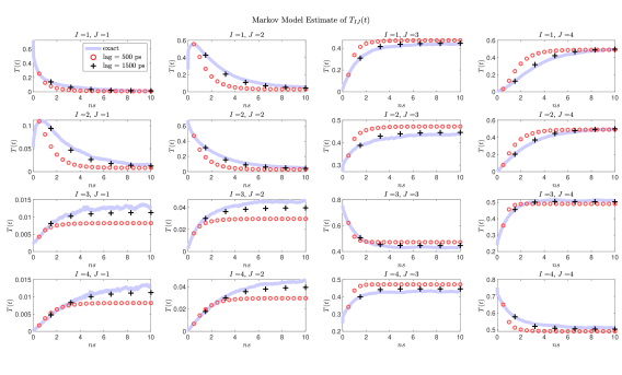
Figure 2: Building a Markov model for alanine dipeptide, using states defined through PCCA. Except at very long lags, the Markov model is considerably less accurate than what we obtain with our methods (see Figure 3). This is because a simple coarse-graining of $X(t)$ into these states is not sufficiently Markovian. Each Markov model is based on a single transition matrix, computed from counts of transitions of $X(t)$ between macrostates at the specified lag time. Transitions at longer lags are computed using powers of this single matrix.

The QSD of $X(t)$ in $I$ is defined by the condition that if $X(t)$ is initially distributed as the QSD in $I$, then conditionally on staying in $I$, it remains distributed as the QSD. Writing $\eta_{I}$ for the QSD in $I$,

$$\eta_{I}(\cdot)=\int\eta_{I}(dx){\mathbb{P}}(X(t)\in\cdot|X(0)=x,\,X(s)\in I,\,s\leq t),$$ (8)

where the variable $x$ represents microstates of $X(t)$.

Under mild assumptions Collet et al. (2013); Champagnat and Villemonais (2023),

$$\|\eta_{I}-{\mathbb{P}}(X(t)\in\cdot\,|\,X(s)\in I,\,s\leq t)\|\leq c_{I}\delta_{I}^{t},$$ (9)

where $c_{I}$ and $\delta_{I}<1$ are constants, and the norm is the total variation of measures. Informally, given that $X(t)$ remains in macrostate $I$, it converges to $\eta_{I}$ at a geometric rate.

In Theorem A.1 of Appendix A, we show that

$$\mathcal{T}(s,t)=O(t\delta^{\sigma})+\sum_{0<r\leq t}\mathcal{P}(r)\mathcal{T}(s,t-r)+\mathcal{F}(t),$$ (10)

where $\mathcal{P}(t)$ is the jump probability matrix of a Markov renewal process, $\mathcal{F}_{IJ}(t)=\delta_{I=J}\sum_{L}\sum_{s>t}\mathcal{P}_{IL}(s)$, and $\delta=\max_{I}\delta_{I}$, $\sigma=\min_{I}\tau_{I}$. It follows that the transition matrices $\mathcal{T}(s,t)$ converge to the transition matrices of a Markov renewal process defined by the jump time distribution $\mathcal{P}(t)$, at a geometric rate in terms of the decorrelation times.

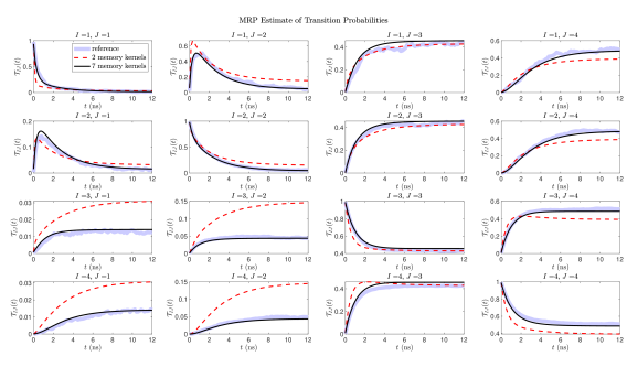
(a) PCCA states

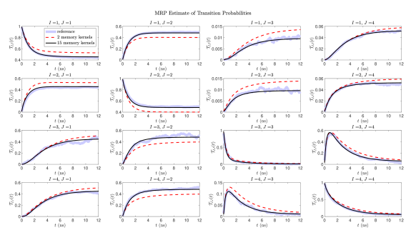
(b) Rectangular states

Figure 3: Results from our method for parametrizing the MRP using (a) states defined by PCCA and (b) equal rectangular states. A very good parameterization is achieved in each case with $7$ and $15$ memory kernels in (a) and (b) respectively. Shown in (a) and (b) are transition probabilities inferred using (7) with a smaller number of memory kernels (dashed line) and a larger number of memory kernels (solid line). The kernels are computed using (5)- (6) with cutoff time twice the memory length ($t_{max}=2t_{mem}$). We use the macroscopic time steps, $\tau=8$ ps (a) and $\tau=30$ ps (b), that define the “good” decorrelation times. (See Figure 4 for the choice of $\tau$ in (a).) Results are clearly improved with the larger number of memory kernels.

V Numerical results

To demonstrate the potential of our method, we apply it to alanine dipeptide, using an MD trajectory Agarwal et al. (2020) of length about $70$ ms. Positions in $\phi$-$\psi$ space were saved at every $2$ ps. The macrostates are either chosen by using PCCA or by dividing $\phi$-$\psi$ space into four equal rectangles. While the PCCA states are highly metastable, the rectangular states are not. A finite spatial discretization limits the accuracy of Markov models, as seen in Figure 2, which shows that a Markov model does not accurately represent the discretized alanine dipeptide dynamics, except at long timescales.

We use a decorrelation time $\tau_{I}=\tau$ ps that is the same for all states $I=1,2,3,4$. These decorrelation times were chosen to be large enough to obtain good numerical accuracy of the renewal equation (2); see Figure 4. Then we construct a trajectory $R(t)$ as described in Section II (see also Figure 1), and apply our method. The alanine MD trajectory was split in half into a training set and a test (or reference) set. We use the former to create our model of $R(t)$, and the latter to create reference results.

To assess our method, we compare it with a reference that uses the indicated value of $\tau$. The reference results are based on simple counts of transitions. Figure 3 compares reference counts with our method’s estimates of $\mathcal{T}(t)$. Figure 5 shows the error in $\mathcal{P}(t)$. To mitigate noise effects from finite sampling, we use the error measurement

$$\begin{split}\textup{Error}&=\sum_{I,J}\int_{0}^{\infty}\left(\int_{0}^{t}\frac{[\mathcal{P}_{IJ}(s)-\hat{\mathcal{P}}_{IJ}(s)]}{Z_{IJ}}ds\right)^{2}\frac{\mathcal{P}_{IJ}(t)}{Z_{IJ}}dt,\end{split}$$ (11)

where $Z_{IJ}=\int_{0}^{\infty}\mathcal{P}_{IJ}(t)\,dt$, and where $\hat{\mathcal{P}}(t)$ is our estimate on training data, with $\mathcal{P}(t)$ the reference. This is a slight variation on the Cramer-von Mises criterion Anderson (1962). Figures 3 and 5 show that the approach outlined in Section III gives good agreement with the reference, with just a few memory kernels.

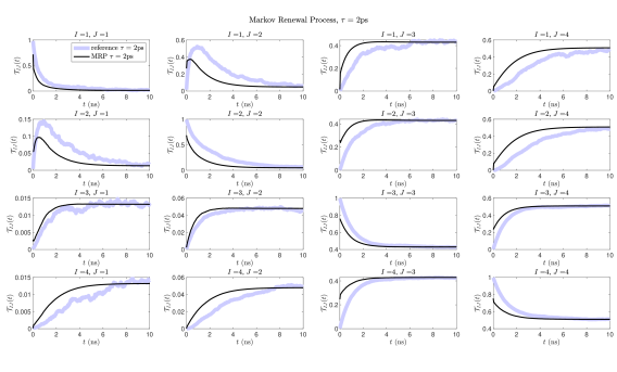
(a) $\tau=2$ps

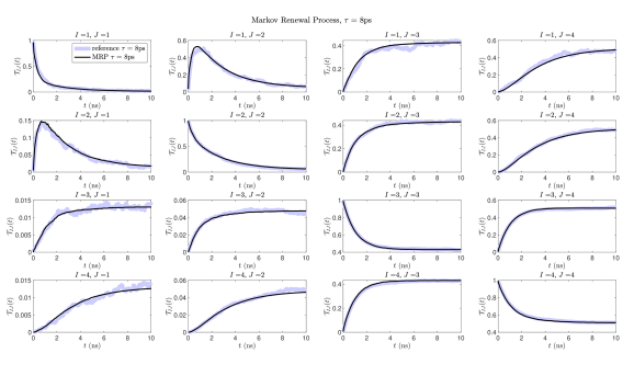
(b) $\tau=8$ps

Figure 4: Verifying that $R(t)$ is approximately a MRP for large enough decorrelation times, for PCCA states. Plotted are reference transition probabilities computed from simple counts of $R(t)$, for $\tau=2$ ps in (a) and $\tau=8$ ps in (b), compared to probabilities computed from the renewal equation (2). (In the renewal equation, the jump probability matrix, $\mathcal{P}$, is similarly computed from simple counts.) The (constant) decorrelation time must be chosen long enough to allow local equilibration within the macrostates. There is significant disagreement using $\tau=2$ ps in (a), while the larger value, $\tau=8$ ps, in (b) gives good agreement without being unnecessarily large.

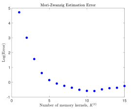
(a) PCCA States, $\tau=8$ ps

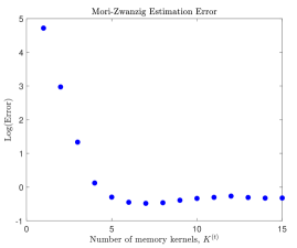
(b) Rectangular States, $\tau=30$ ps

Figure 5: The error in our method vs. the number of memory kernels. Memory kernels are estimated at multiples of $\tau$ and the error is defined by (11). The cutoff times, (a): $t_{max}=120$ ps and (b): $t_{max}=900$ ps, are chosen by applying the rule $t_{mem}=0.5\times t_{max}$ to the largest $t_{mem}$ pictured (for instance in (b) $t_{mem}=450$ ps, corresponding to $15$ memory kernels).

Practical considerations

Our method requires a choice of macrostates and of scalar parameters $\tau$, $t_{mem}$ and $t_{max}$. Here, we discuss how these parameters might be chosen. Briefly, the microstates should be chosen as metastable states associated with timescales of interest; the parameter $\tau$ should be large enough for the Markov property to (nearly) hold, but no larger; and $t_{mem}$ and $t_{max}$ should be as large as needed to accurately parametrize the model, given constraints on how much data is available. We discuss all this in more detail below. In this discussion, as in the numerical simulations, we assume that all the decorrelation times equal $\tau$, that is, $\tau_{I}=\tau$ for each macrostate $I$.

We first consider $\tau$, $t_{mem}$ and $t_{max}$. With enough data, increasing $\tau$, $t_{mem}$ and $t_{max}$ will systematically improve results; in practice, though, there are tradeoffs. (Caveat: a too large $\tau$ causes modeling problems; see below.) Clearly, there need to be enough sampled transitions at each time lag. That is, we need enough samples of $\mathcal{T}_{IJ}(t)$ for each $I,J$ and $t\leq t_{max}$. So for example, if data comes in the form of many short trajectories of $X(t)$, then increasing $t_{max}$ lowers transition counts, and can improve model fidelity only to the extent that the number of sampled transitions does not get too low. The parameter $t_{mem}$ defines the number of memory kernels, and we found good results when pairing it to $t_{max}$ using the rule $t_{mem}\approx 0.5\times t_{max}$. In practice, $t_{max}$ (and/or $t_{mem}$) could be chosen with standard techniques like cross-validation.

The macrostates and the parameter $\tau$ are more fundamental (though they are also subject to similar considerations concerning transition counts). Unlike $t_{mem}$ and $t_{max}$, which are parameters used to obtain the memory kernels which generate an approximation of $R(t)$, the macrostates and $\tau$ actually define $R(t)$. They must be chosen carefully to yield good results. For a given set of macrostates, a minimum value of $\tau$ is set by the requirement that $R(t)$ is approximately a MRP; the required value can be found empirically by using a plot like Figure 4 (we simply chose one “by eye” from such plots). Good macrostates are ones in which decorrelation occurs on a time scale much smaller than the typical escape time – i.e., good macrostates are metastable Lelièvre (2015). In practice, they could be chosen by standard techniques like PCCA Chodera and Noé (2014).

A bad choice of macrostates cannot be rescued by a good choice of $\tau$. Indeed, $R(t)$ does not retain any events that occur on timescales smaller than $\tau$. As a result, if $\tau$ is close or larger than typical transition times between macrostates, then $R(t)$ can miss such transitions (as shown in Figure 1), resulting in a potentially accurate but uninformative model. A good choice of both the macrostates and of $\tau$ is therefore important. For the purposes of this article, we think of the macrostates as already being given, and we choose $\tau$ by looking at plots like Figure 4, increasing $\tau$ until we find a good match.

Figure 2 shows an ordinary Markov model based on PCCA states. These PCCA states are the same as reference Agarwal et al. (2020). A lag of $1500$ ps is needed for accuracy comparable to our methods. (Compare with Figure 3(a).) This lag is on the order of the longest mean transition time, roughly $1000$ ps. Particularly for macrostates 1 and 2, this lag sacrifices knowledge of shorter timescale (but still physically relevant) state-to-state transitions. Although these states are considered very good (Markovian) states, our methods still provide significant improvement over Markov models, as illustrated in Figure 3.

Figure 3(a) shows results from our methods when using the PCCA states. There, we use a decorrelation time $\tau=8$ ps. This serves as the fundamental time step of our coarse-grained model, and is small enough that few transitions are missed. To build our model, we use many short trajectories of length $112$ ps, smaller than the shortest mean transition time of $175$ ps. (This trajectory length corresponds to using $\tau=8$ ps, with $t_{mem}=7$ memory kernels and $t_{max}=2\times t_{mem}$.) In contrast, a similarly accurate Markov model in Figure 2 requires trajectories of length $1500$ ps. Recall that the longest mean transition time is around $1000$ ps. In sum, the renewal model requires significantly shorter trajectories and is more accurate than the Markov model on all timescales.

Figure 3(b) shows analogous results for unphysical macrostates (defined as equal rectangles in $\phi$-$\psi$ coordinates, divided by the lines $\phi=0,\pm\pi$ and $\psi=0,\pm\pi$). Although these states are no longer metastable, results are similar to Figure 3(a). (In this case $\tau$ needs to be larger, however, resulting in our model missing some transitions, as discussed above.) We find good accuracy when $\tau=30$ ps, $t_{mem}=15$ memory kernels, and trajectories have length $900$ ps. A Markov model would require a lag of $5000$ ps for similar accuracy. Smaller Markov model lags of $\sim 1000$ ps result in wildly inaccurate estimates for even a few time steps’ prediction.

VI Discussion

The methodology introduced in this paper allows for the systematic exploitation of a rich set of trade-offs between compactness, expressiveness, and accuracy. It is particularly well suited to cases where the system contains a relatively small number of metastable states, but where metastability is insufficient for a Markovian assumption to be accurate. In contrast to conventional approaches like Markov State Models, where accuracy can be improved by increasing the number of states at the cost of interpretability, the accuracy of the approach proposed is instead controlled by increasing the decorrelation time, to ensure the convergence to a MRP. Doing so however comes with its own trade-off, as the expressiveness of $R(t)$ decreases when the decorrelation time exceeds the shortest transition time. However, the geometric convergence rate to an MRP makes this trade-off particularly advantageous as a small increase in decorrelation time yields a large increase in accuracy. Therefore, even for modestly metastable systems, it should be possible to produce very accurate MRPs using decorrelation times that are short compared to typical transition times, hence minimizing the loss of kinetic information. In this situation, the MZ approach described above will also yield a compact representation in terms of a limited number of kernel matrices. As shown above, this approach allows one to obtain compact and accurate models even with sub-optimal state definitions, which is very useful given that optimizing state definitions in high dimension is generally difficult. That being said, the approach cannot fix state definitions where most of the states are not at least somewhat metastable, as accuracy would demand very long decorrelation times, which would then entail low expressiveness. It is arguable, however, that no representation in terms of jump processes would be appropriate in such a scenario.

Appendix A Convergence to a Markov renewal process

We begin by introducing some notation. Let

$$E_{IJ}(s,t)=\{R(s+t)=J,\,R(s^{\prime})=I,\,s\leq s^{\prime}<s+t\}$$

be the event of switching to from $I$ to $J$ after a time $t$, starting from time $s$. Let

$$E_{J}(t)=\{R(t)=J\},\qquad E_{J}^{c}(t)=\{R(t)\neq J\}$$

be the events that $R(t)=J$ and $R(t)\neq J$, respectively.

We use $\sim$ to indicate equality in distribution; for example, $X(s)\sim\eta_{I}$ indicates that $X(s)$ is distributed as $\eta_{I}$.

The following result demonstrates convergence in distribution of $R(t)$ to a Markov renewal process as the decorrelation times grow.

Theorem A.1 (Exactness of renewal equation).

Assume that each macrostate $I$ has a QSD $\eta_{I}$, and assume that (9) holds. Define

$$\mathcal{T}_{IJ}(t)={\mathbb{P}}(E_{J}(s+t)|E_{I}(s),\,X(s)\sim\eta_{I}).$$ (12)

Then $\mathcal{T}(s,t)$ defined by (1) converges to $\mathcal{T}(t)$ defined by (12) as $\min_{I}\tau_{I}\to\infty$. Moreover, the limit $\mathcal{T}(t)$ is the unique solution to the renewal equation (2) when $\mathcal{P}$ is defined by

$$\begin{split}\mathcal{P}_{IJ}(t)&=\delta_{I\neq J}{\mathbb{P}}(E_{IJ}(s,t)|E_{I}(s),\,X(s)\sim\eta_{I}).\end{split}$$ (13)

Proof.

Using the law of total probability,

$$\begin{split}\mathcal{T}_{IJ}(s,t)&={\mathbb{P}}(E_{J}(s+t)|E_{I}^{c}(s_{-}),\,E_{I}(s))\\ &=\sum_{K\neq I}\sum_{0<r\leq t}{\mathbb{P}}(E_{J}(s+t)|E_{I}^{c}(s_{-}),E_{IK}(s,r))\\ &\qquad\qquad\times{\mathbb{P}}(E_{IK}(s,r)|E_{I}^{c}(s_{-}),\,E_{I}(s))\\ &+\delta_{I=J}{\mathbb{P}}(E_{II}(s,t)|E_{I}^{c}(s_{-}),\,E_{I}(s)).\end{split}$$ (14)

Let $\sigma=\min_{I}\tau_{I}$, and in the notation of (9), define

$$c=\max_{I}c_{I},\quad\delta=\max_{I}\delta_{I}.$$

Using (9), (12), and the Markov property of $X(t)$,

$$\begin{split}\mathcal{T}_{IJ}(s,t)&={\mathbb{P}}(E_{J}(s+t)\,|\,E_{I}^{c}(s_{-}),\,E_{I}(s))\\ &=\int{\mathbb{P}}(E_{J}(s+t)\,|\,E_{I}^{c}(s_{-}),\,E_{I}(s),\,X(s)=x)\\ &\qquad\quad\times{\mathbb{P}}(X(s)\in dx\,|\,E_{I}^{c}(s_{-}),\,E_{I}(s))\\ &=\int{\mathbb{P}}(E_{J}(s+t)\,|\,E_{I}(s),\,X(s)=x)\nu_{I}(dx)+\epsilon_{I}\\ &=\mathcal{T}_{IJ}(t)+\epsilon,\end{split}$$ (15)

where $|\epsilon|\leq c\delta^{\sigma}$. Similar calculations show that

$$\delta_{I\neq K}{\mathbb{P}}(E_{J}(s+t)|E_{I}^{c}(s_{-}),E_{IK}(s,r))=\mathcal{T}_{KJ}(t-r)+\epsilon$$

$$\delta_{I\neq K}{\mathbb{P}}(E_{IK}(s,r)|E_{I}^{c}(s_{-}),\,E_{I}(s))=\mathcal{P}_{IK}(r)+\epsilon$$

$${\mathbb{P}}(E_{II}(s,t)|E_{I}^{c}(s_{-}),\,E_{I}(s))=\mathcal{F}_{II}(t)+\epsilon,$$

where each $\epsilon$ is different but $|\epsilon|\leq c\delta^{\sigma}$, and

$$\mathcal{F}_{IJ}(t) =\delta_{I=J}{\mathbb{P}}(E_{II}(s,t)|E_{I}(s),\,X(s)\sim\nu_{I})$$

$$=\delta_{I=J}\sum_{L}\sum_{s>t}\mathcal{P}_{IL}(s).$$

Combining the previous three displays with (14),

$$\mathcal{T}(s,t)=O(t\delta^{\sigma})+\sum_{0<r\leq t}\mathcal{P}(r)\mathcal{T}(s+r,t-r)+\mathcal{F}(t).$$ (16)

Now from (15), we conclude that $\mathcal{T}(s,t)$ converges to $\mathcal{T}(t)$ as $\sigma\to\infty$. Meanwhile, using (16), it is readily shown from a standard renewal equation representation (Cinlar, 1975, Proposition 4.2) that $\mathcal{T}(t)$ is the unique solution to equation (2). ∎

The proof shows that the convergence rate is geometric in $\sigma$ on finite time intervals, suggesting that large decorrelation times are not needed in order to model $R(t)$ as a Markov renewal process, at least for reasonably defined states.

Appendix B Actions of projector and Markov kernels

Below, we introduce another process $C(t)$ that counts the consecutive time that $X(t)$ has spent in its current macrostate, where the count stops at $\tau_{J}$ if $X(t)\in J$.

To develop the Mori Zwanzig theory, we introduce the augmented Markov chain $(X(t),R(t),C(t))$ on augmented states $(x,I,s)$, where $x$ and $I$ represent the current values of $X(t)$ and $R(t)$, and $s$ is the consecutive time that $X(t)$ has spent in the macrostate in which it currently resides, up to the decorrelation time. This Markov chain has time step $\tau$.

Below, let ${\mathbb{P}}^{x,I,s}$ denote probability for the augmented Markov chain that starts at $(X(0),R(0),C(0))=(x,I,s)$. Let $T$ be the Markov kernel of this augmented chain,

$$\begin{split}&T(x,I,s;dy,J,t)\\ &\qquad={\mathbb{P}}^{x,I,s}[(X(\tau),R(\tau),C(\tau))=(dy,J,t)].\end{split}$$ (17)

We will also make use of more broadly defined kernels $S(x,I,s;dy,J,t)$ by relaxing the nonnegativity and unit normalization properties of $T$. Specifically, such a kernel acts on functions $f=f(x,I,s)$ of augmented space according to the rule

$$Sf(x,I,s)=\int\sum_{J,t}S(x,I,s;dy,J,t)f(y,J,t).$$

We define a projector $P$ on functions $f=f(x,I,s)$ of augmented states, that is, a mapping satisfying $P^{2}=P$, by

$$Pf(x,I,s)=\int\eta_{I}(dz)f(z,I,\tau_{I}).$$ (18)

Appendix C Principal and orthogonal dynamics, and Markovian case

The Mori-Zwanzig theory is characterized by a principal and orthogonal dynamics. The principal dynamics is driven by $PT$, defined by

$$PT(x,I,s;dy,J,t)=\int\eta_{I}(dz)T(z,I,\tau_{I};dy,J,t).$$

The orthogonal dynamics is driven by $QT$, where $Q=\textup{Id}-P$ and Id is the identity operator; that is, $QT=T-PT$.

We consider a special Markovian case, in which the underlying dynamics instantaneously reaches the QSD in whatever macrostate it resides in, with associated decorrelation times $\tau_{I}=0$ for all $I$. In this case, $T=PT$, so the orthogonal dynamics vanish, $QT=0$, and all but one of the memory kernels is zero; see Appendix D.

Appendix D Derivation of the Mori Zwanzig equation

The following lemma applies to any transition kernel $T$ and projector $P$, although we have in mind the Markov kernel $T$ in (LABEL:eq:T) and the projector $P$ in (18).

Lemma D.1.

For any projector $P$ and its complementary projector $Q=\textup{Id}-P$, where $Id$ is the identity mapping, we have

$$PT^{n}=\sum_{m=1}^{n}K(m)PT^{n-m}+F(n),$$ (19)

where $K(n)=PT(QT)^{n-1}$ and $F(n)=PT(QT)^{n-1}Q$.

Proof.

Start with the self-evident equations

$$PT^{n+1} =PTPT^{n}+PTQT^{n}$$ (20)

$$QT^{n+1} =QTPT^{n}+QTQT^{n}.$$ (21)

Using induction in (21),

$$QT^{n}=\sum_{m=1}^{n}(QT)^{m}PT^{n-m}+(QT)^{n}Q.$$

Plugging this back into (20) yields the result.∎

Below, we will make use of functions $\chi_{J}$ defined by

$$\chi_{J}(x,I,s)=\delta_{I=J}.$$

Theorem D.2 (Exactness of MZ equation).

Let $K(n)$ be as in Lemma D.1, where $P$ is the projector from (18) and $T$ is defined in (LABEL:eq:T). Define

$$\mathcal{K}_{IJ}(n\tau):=K(n)\chi_{J}(x,I,s).$$ (22)

Then, with $\mathcal{T}(t)$ as in (12),

$$\mathcal{T}(n\tau)=\sum_{m=1}^{n}\mathcal{K}(m\tau)\mathcal{T}((n-m)\tau).$$ (23)

Proof.

Multiply (19) on the right by $\chi_{J}(x,I,s)$. Note that $P\chi_{J}=\chi_{J}$, so that $Q\chi_{J}=0$ and $F(n)\chi_{J}(x,I,s)=0$. Thus,

$$PT^{n}\chi_{J}(x,I,s)=\sum_{m=1}^{n}K(m)PT^{n-m}\chi_{J}(x,I,s).$$ (24)

Recalling $\mathcal{T}(t)$ defined in (12), we compute

$$PT^{n}\chi_{J}(x,I,s) =\int\eta_{I}(dx)T^{n}\chi_{J}(x,I,\tau_{I})$$

$$=\int\eta_{I}(dx)\mathbb{E}^{x,I,\tau_{I}}[\chi_{J}(X(n\tau),R(n\tau),C(n\tau))]$$

$$=\int\eta_{I}(dx){\mathbb{P}}^{x,I,\tau_{I}}[R(n\tau)=J]$$

$$=\mathcal{T}_{IJ}(n\tau).$$

Below, write $S_{m}=T(QT)^{m-1}$, and note that $PT^{n-m}\chi_{J}(y,L,t)$ does not depend on $y$ or $t$. Thus,

$$\sum_{L}\mathcal{K}_{IL}(m\tau)\mathcal{T}_{LJ}((n-m)\tau)$$

$$=\sum_{L}K(m)\chi_{L}(x,I,s)PT^{n-m}\chi_{J}(y,L,t)$$

$$=\sum_{L}\int\eta_{I}(dz)\left[\int\sum_{t}S_{m}(z,I,\tau_{I};dy,L,t)\right]PT^{n-m}\chi_{J}(y,L,t)$$

$$=\int\eta_{I}(dz)\left[\int\sum_{L,t}S_{m}(z,I,\tau_{I};dy,L,t)PT^{n-m}\chi_{J}(y,L,t)\right]$$

$$=K(m)PT^{n-m}\chi_{J}(x,I,s).$$

Combining the last two displays with (24) gives (23). ∎

Next, we show that all but one of the memory kernels vanishes in the case where $R(t)$ is Markovian.

Theorem D.3.

Suppose that $\tau_{I}=0$ for all $I$ and that

$$T(x,I,s;dy,J,t)=\int\nu_{I}(dz)T(z,I,\tau_{I};dy,J,t).$$

Then $\mathcal{K}(n\tau)=0$ for $n>1$.

Proof.

The assumption on $T$ implies that $PT=T$, so $QT=0$ and the result follows from the formula

$$\mathcal{K}_{IJ}(n\tau)=PT(QT)^{n-1}\chi_{J}(x,I,s).$$

∎

Appendix E Minimizing the loss function

The gradient of the loss function (4) is

$$\nabla_{\mathcal{K}(t)}{\mathcal{L}}(\mathcal{K}) =\sum_{r\leq t_{max}}\mathcal{T}(r)\mathcal{T}(r-t)^{T}$$

$$\qquad-\sum_{0<s\leq t_{mem}}\mathcal{K}(s)\sum_{r\leq t_{max}}\mathcal{T}(r-s)\mathcal{T}(r-t)^{T},$$

where by definition $\mathcal{T}(s)=0$ for $s<0$.

This immediately leads to the linear system reported in (5).

References

- Karplus and Petsko (1990) M. Karplus and G. A. Petsko, Nature 347, 631 (1990).
- Karplus and McCammon (2002) M. Karplus and J. A. McCammon, Nature structural biology 9, 646 (2002).
- Hansson et al. (2002) T. Hansson, C. Oostenbrink, and W. van Gunsteren, Current opinion in structural biology 12, 190 (2002).
- Durrant and McCammon (2011) J. D. Durrant and J. A. McCammon, BMC biology 9, 1 (2011).
- Hospital et al. (2015) A. Hospital, J. R. Goñi, M. Orozco, and J. L. Gelpí, Advances and applications in bioinformatics and chemistry , 37 (2015).
- Hollingsworth and Dror (2018) S. A. Hollingsworth and R. O. Dror, Neuron 99, 1129 (2018).
- Chong et al. (2017) L. T. Chong, A. S. Saglam, and D. M. Zuckerman, Current opinion in structural biology 43, 88 (2017).
- Weare (2009) J. Weare, Journal of Computational Physics 228, 4312 (2009).
- Webber et al. (2019) R. J. Webber, D. A. Plotkin, M. E. O’Neill, D. S. Abbot, and J. Weare, Chaos: An Interdisciplinary Journal of Nonlinear Science 29, 053109 (2019).
- Finkel et al. (2023a) J. Finkel, R. J. Webber, E. P. Gerber, D. S. Abbot, and J. Weare, Journal of the Atmospheric Sciences 80, 519 (2023a).
- Finkel et al. (2023b) J. Finkel, E. P. Gerber, D. S. Abbot, and J. Weare, AGU Advances 4, e2023AV000881 (2023b).
- Seiden and Thomas (2011) G. Seiden and P. J. Thomas, Reviews of Modern Physics 83, 1323 (2011).
- Fingelkurts and Fingelkurts (2004) A. A. Fingelkurts and A. A. Fingelkurts, International Journal of Neuroscience 114, 843 (2004).
- Haldeman and Beggs (2005) C. Haldeman and J. M. Beggs, Physical review letters 94, 058101 (2005).
- Hellyer et al. (2015) P. J. Hellyer, G. Scott, M. Shanahan, D. J. Sharp, and R. Leech, Journal of Neuroscience 35, 9050 (2015).
- Córdova-Palomera et al. (2017) A. Córdova-Palomera, T. Kaufmann, K. Persson, D. Alnæs, N. T. Doan, T. Moberget, M. J. Lund, M. L. Barca, A. Engvig, A. Brækhus, et al., Scientific reports 7, 1 (2017).
- Naik et al. (2017) S. Naik, A. Banerjee, R. S. Bapi, G. Deco, and D. Roy, Trends in cognitive sciences 21, 509 (2017).
- Cavanna et al. (2018) F. Cavanna, M. G. Vilas, M. Palmucci, and E. Tagliazucchi, Neuroimage 180, 383 (2018).
- Pomeau (1986) Y. Pomeau, Physica D: Nonlinear Phenomena 23, 3 (1986).
- Matthews et al. (2018) C. Matthews, B. Stadie, J. Weare, M. Anitescu, and C. Demarco, arXiv preprint arXiv:1806.02420 (2018).
- Duncan and Dunwell (2002) D. B. Duncan and R. M. Dunwell, Proceedings of the Edinburgh Mathematical Society 45, 701 (2002).
- Sun and Ward (1999) X. Sun and M. J. Ward, European Journal of Applied Mathematics 10, 27 (1999).
- Estep (1994) D. Estep, Nonlinearity 7, 1445 (1994).
- Groisman et al. (2018) P. Groisman, S. Saglietti, and N. Saintier, Stochastic Processes and their Applications 128, 1558 (2018).
- Norris (1998) J. R. Norris, Markov chains, 2 (Cambridge university press, 1998).
- Durrett and Durrett (1999) R. Durrett and R. Durrett, Essentials of stochastic processes, Vol. 1 (Springer, 1999).
- Angeli (2009) D. Angeli, in 2009 European Control Conference (ECC) (IEEE, 2009) pp. 649–657.
- Voter (2007) A. F. Voter, in Radiation effects in solids (Springer, 2007) pp. 1–23.
- Chodera and Noé (2014) J. D. Chodera and F. Noé, Current opinion in structural biology 25, 135 (2014).
- Bortz et al. (1975) A. B. Bortz, M. H. Kalos, and J. L. Lebowitz, Journal of Computational Physics 17, 10 (1975).
- Gillespie (1977) D. T. Gillespie, The journal of physical chemistry 81, 2340 (1977).
- Husic and Pande (2018) B. E. Husic and V. S. Pande, Journal of the American Chemical Society 140, 2386 (2018).
- Di Gesù et al. (2016) G. Di Gesù, T. Lelièvre, D. Le Peutrec, and B. Nectoux, Faraday discussions 195, 469 (2016).
- Ross (1995) S. M. Ross, Stochastic processes (John Wiley & Sons, 1995).
- Brémaud (2001) P. Brémaud, Markov chains: Gibbs fields, Monte Carlo simulation, and queues, Vol. 31 (Springer Science & Business Media, 2001).
- Lelièvre (2015) T. Lelièvre, The European Physical Journal Special Topics 224, 2429 (2015).
- Lelièvre (2020) T. Lelièvre, Handbook of Materials Modeling: Methods: Theory and Modeling , 773 (2020).
- Cinlar (1975) E. Cinlar, Management Science 21, 727 (1975).
- Agarwal et al. (2020) A. Agarwal, S. Gnanakaran, N. Hengartner, A. F. Voter, and D. Perez, arXiv preprint arXiv:2008.11623 (2020).
- Darve et al. (2009) E. Darve, J. Solomon, and A. Kia, Proceedings of the National Academy of Sciences 106, 10884 (2009).
- Cao et al. (2020) S. Cao, A. Montoya-Castillo, W. Wang, T. E. Markland, and X. Huang, The Journal of Chemical Physics 153, 014105 (2020).
- Lin et al. (2022) Y. T. Lin, Y. Tian, D. Perez, and D. Livescu, arXiv preprint arXiv:2205.05135 (2022).
- Chen et al. (2022) Y. Chen, E. N. Epperly, J. A. Tropp, and R. J. Webber, arXiv preprint arXiv:2207.06503 (2022).
- Díaz et al. (2023) M. Díaz, E. N. Epperly, Z. Frangella, J. A. Tropp, and R. J. Webber, arXiv preprint arXiv:2304.12465 (2023).
- Lin et al. (2021) Y. T. Lin, Y. Tian, D. Livescu, and M. Anghel, SIAM Journal on Applied Dynamical Systems 20, 2558 (2021).
- Dominic III et al. (2023a) A. J. Dominic III, T. Sayer, S. Cao, T. E. Markland, X. Huang, and A. Montoya-Castillo, Proceedings of the National Academy of Sciences 120, e2221048120 (2023a).
- Dominic III et al. (2023b) A. J. Dominic III, S. Cao, A. Montoya-Castillo, and X. Huang, Journal of the American Chemical Society (2023b).
- Collet et al. (2013) P. Collet, S. Martínez, and J. San Martín, Quasi-stationary distributions: Markov chains, diffusions and dynamical systems, Vol. 1 (Springer, 2013).
- Champagnat and Villemonais (2023) N. Champagnat and D. Villemonais, Electronic Journal of Probability 28, 1 (2023).
- Anderson (1962) T. W. Anderson, The Annals of Mathematical Statistics , 1148 (1962).