Observation of a dissipative time crystal in a strongly interacting Rydberg gas
Abstract
The notion of spontaneous symmetry breaking has been well established to characterize classical and quantum phase transitions of matter, such as in condensation, crystallization or quantum magnetism. Generalizations of this paradigm to the time dimension can lead to an exotic dynamical phase, the time crystal, which spontaneously breaks the time translation symmetry of the system Wilczek (2012). While the existence of a continuous time crystal at equilibrium has been challenged by no-go theorems Nozières (2013); Bruno (2013); Watanabe and Oshikawa (2015), the difficulty can be circumvented by dissipation in an open system. Here, we report the experimental observation of such dissipative time crystalline order in a room-temperature atomic gas, where ground-state atoms are continuously driven to Rydberg states. The emergent time crystal is revealed by persistent oscillations of the photon transmission, with no observable damping during the measurement. We show that the observed limit cycles arise from the coexistence and competition between distinct Rydberg components, in agreement with a mean-field analysis derived from the microscopic model. The nondecaying autocorrelation of the oscillation, together with the robustness against temporal noises, indicates the establishment of true long-range temporal order and demonstrates the realization of a continuous time crystal in our experiments.
The search for emergent many-body phases is among the central objectives of quantum physics Sondhi et al. (1997). While the concept of phase transitions in thermal equilibrium is well developed, the presence of driving and dissipation can result in a rich phenomenology that has no counterpart in equilibrium Eisert et al. (2015), such as ubiquitous self-organization effects in physics, biology, and economics Haken (2006). In particular, such nonequilibrium processes can facilitate a novel dynamical phase that spontaneously breaks time translation symmetry Keßler et al. (2019); Buča et al. (2019); Dogra et al. (2019); Dreon et al. (2022), commonly referred to as a time crystal Shapere and Wilczek (2012); Sacha and Zakrzewski (2017); Zhang et al. (2017); Choi et al. (2017); Rovny et al. (2018); Riera-Campeny et al. (2020); Randall et al. (2021); Kyprianidis et al. (2021); Keßler et al. (2021); Mi et al. (2022); Taheri et al. (2022). In analogy to crystals in space, a continuous time crystal (CTC) phase has an order parameter with self-sustained oscillations, even though the system is driven in a continuous manner Iemini et al. (2018); Bakker et al. (2022); Carollo and Lesanovsky (2022); Krishna et al. (2023); Nie and Zheng (2023). Remarkably, the spontaneous time translation symmetry breaking associated with a dissipative CTC has been recently observed with atomic Bose-Einstein condensate in an optical cavity Kongkhambut et al. (2022). The inevitable loss of atoms in the ultracold regime, however, complicates the investigation of long-time dynamics and thereby hinders the analysis of long-range time crystalline order.
Ensembles of Rydberg atoms represent a suitable platform for exploring many-body phenomena away from equilibrium emerging from coherent driving, dissipation, and long-range dipole-dipole interactions Carr et al. (2013); Malossi et al. (2014); Ding et al. (2020); Wu et al. (2021); Horowicz et al. (2021); Franz et al. (2022). Such a Rydberg gas is well controllable and can be confined in a room-temperature vapour cell at virtually no atom loss. Here, we exploit this feature and report the experimental observation of long-range time crystalline order in a continuously driven Rydberg gas [see Fig. 1(a)]. In our experiment, the CTC manifests itself in limit cycle oscillations of the Rydberg atom density and the atomic dipole moment, which we probe directly by the transmission of light through the gas [see Fig. 1(b)]. We demonstrate that the time crystal originates from the competition between atomic excitations in different Rydberg states, and characterize the parameter regimes that support this phase. We verify the observation of a CTC by experimentally demonstrating the establishment of a long-range autocorrelation function and its robustness against noisy temporal perturbations.
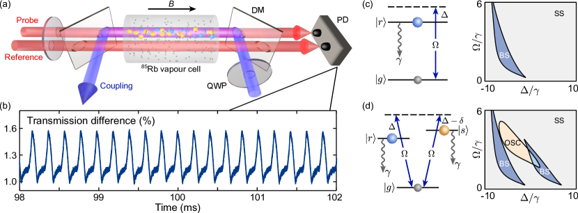
To understand the origin of the limit cycle in our experiment, we first consider the microscopic description of the driven-dissipative Rydberg gas. As illustrated in Fig. 1(c), the applied laser fields generated a coherent coupling between the atomic ground state and a Rydberg state , with a corresponding Rabi frequency and frequency detuning , while spontaneous decay leads to a loss of coherence and Rydberg population with a rate . The strong interaction between Rydberg states is governed by a Hamiltonian , with the local Rydberg density and the van der Waals interaction between Rydberg atoms located at and . In a thermal Rydberg gas, however, the atomic motion averages out the associated spatial correlations between Rydberg atoms and permits a mean-field treatment of the interaction Carr et al. (2013), whereby the laser detuning acquires a dependence on the uniform Rydberg density , with an effective nonlinearity strength . The finite decay rate usually relaxes the system to a stationary mixed state (SS), corresponding to the fixed point of the nonlinear optical Bloch equation. However, it has been shown that the interaction induced nonlinearity can cause a saddle-node bifurcation Carr et al. (2013), through which a bistable stationary state emerges in a finite region of the parameter space. For an attractive interaction (), such a bistable phase (BS) can occur at the negative detuning regime [see the right panel of Fig. 1(c)]. At its boundaries one finds a discontinuous nonequilibrium transition between distinct stationary states with low and high Rydberg-state concentration, respectively.
The situation changes dramatically when more than one Rydberg states come into play. In order to illustrate this effect, we consider a minimal extension, in which one additional Rydberg state is coupled with an identical Rabi frequency but different detuning , [see Fig. 1(d)]. These distinct Rydberg states can establish their respective bistable phases at different detunings for a sufficiently large energy separation . More importantly, their strong interactions generate nonlinear energy shifts, , that couple the dynamics of both Rydberg states (see Methods). The resulting competition can drive a Hopf bifurcation for , whereby a non-stationary dynamical phase appears in between the two bistable regions, as illustrated in the right panel of Fig. 1(d). In this non-stationary regime, the interaction can facilitate the excitation of one Rydberg state at the cost of the other, leading to limit cycle dynamics with persistent oscillations of the Rydberg densities without damping.
The experimental setup for observing such an oscillatory dynamics is depicted in Fig. 1(a), where 85Rb atoms are trapped in a room-temperature vapour cell. The atoms are continuously excited to the Rydberg states via a two-photon process, in which a probe beam and a coupling beam counterpropagates with each other. Here, the probe and the coupling fields drive the ground state manifold to the Rydberg manifold () via intermediate states . The exact Zeeman level of the states can be specified by the polarization of the beams [see Fig. 2(a)]. In the limit cycle phase, the dynamics imposes an oscillation of the transition dipoles between these states, which results in an oscillating transmission of the probe field. To obtain a clear transmission signal, we use a calcite beam displacer to generate a reference beam parallel to the probe beam for differential measurement. The transmission signal for a high lying Rydberg state with a principal quantum number is shown in Fig. 1(b), which exhibits a stable periodic oscillation pattern. In this single experiment, three Rydberg states close in energy are involved in the driving scheme Su et al. (2022), and should all participate in the synchronized oscillating dynamics.
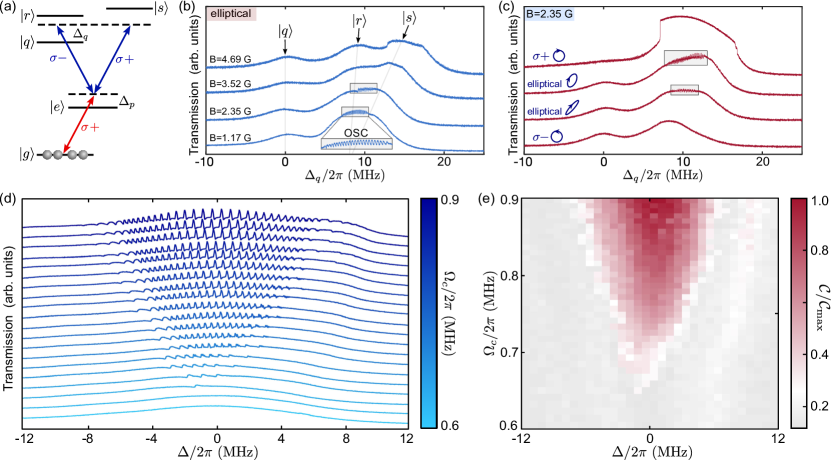
To confirm that the oscillation is indeed induced by the involvement of multiple Rydberg states, we reduce the principal quantum number to and apply a magnetic field to adjust the energy differences between distinct Zeeman levels. Then, with a careful choice of the polarization, we can study the dynamics mainly involving two Rydberg states close in energy, i.e., states and in Fig. 2(a). The branching ratio of the coupling to these states can be tuned by the polarization of the coupling field Su et al. (2022). In order to identify the region displaying limit cycles, we perform a scanning spectroscopy measurement, in which the frequency of the coupling beam is slowly scanned near the two-photon resonance with a fixed intermediate-state detuning . In the scanning process, the magnetic insensitive Rydberg level separated from the two target states can also be laser coupled, and is chosen as a reference state with a detuning .
The observed transmission spectrum for different magnetic fields and polarizations are shown in Figs. 2(b) and 2(c). First, we set the polarization of coupling beam to be elliptical, by which both Rydberg states can be excited, and they are distinguishable at a large magnetic field [see Fig. 2 (b)]. Crucially, oscillations appear only in the case of a relatively small magnetic field, where and are close enough to induce the competition. Next, we fix the magnetic field at a small value and vary the polarization of the coupling light [see Fig. 2(c)]. We find the oscillating phase only exists at an elliptical polarization, but disappears for a perfectly circularly polarized case or , where only one of the Rydberg states or is excited. Based on this experimental evidence, we can conclude that it is the competition between multiple Rydberg levels facilitating the limit cycle phase, in agreement with the mean-field prediction.
In addition to multiple Rydberg components, sufficiently large Rabi frequencies of the probe () and the coupling () are also necessary to induce the limit cycle. Figure 2(d) displays the transmission spectrum at different with a large and fixed , from which rich oscillating patterns can be identified. First, we note that the oscillation completely disappears if the Rabi frequency is too small. Then, weak and long-period oscillations come into appearance when slightly exceeds a certain critical point. As the Rabi frequency is further increased, the amplitude of the oscillation as well as its range increases. Choosing the oscillating contrast ratio as the order parameter, we can extract an approximate phase diagram from the transmission spectrum, as shown in Fig. 2(e), where limit cycle phase is revealed by a nonvanishing contrast. The measured phase diagram indicates that the limit cycle phase exists over a wide parameter regimes and is not sensitive to experimental conditions, such as laser power and frequency, etc.
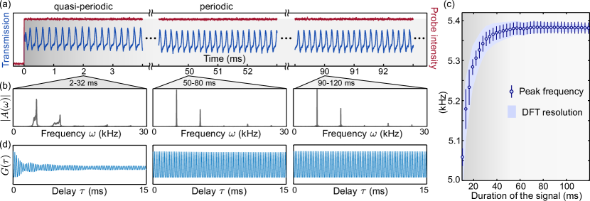
Having identified parameter regions that support oscillatory states, we can now study their properties in relation to the physics of time crystals. Specifically, we investigate a quench dynamics, where the probe field is suddenly turned on and then held at a constant strength for a very long time. As a typical realization shown in Fig. 3(a), the elementary oscillation pattern is rapidly established within , and then sustained in the entire driving window of . A detailed analysis of the signal reveals that the oscillation is initially quasi-periodic and synchronizes steadily to a periodic one. Figure 3(b) displays the discrete Fourier transform (DFT) of the transmission signal at different stages. For the time window 2-32 ms, the Fourier spectrum has several broad peaks, indicating the absence of a well-defined periodicity. In contrast, the spectrum features equally separated narrow spikes for the time window 50-80 ms and remains its shape for a lagged copy 90-120 ms, suggesting that a stable periodic pattern has been reached and maintained. We then perform 100 independent measurements and study evolution of the oscillation frequencies. As shown in Fig. 3(c), the fundamental frequency drifts towards higher values in the quasi-periodic region, and then converges to a stable one. These repeated realizations of the quench dynamics confirm that the above evolution towards a stable oscillating periodicity is not a consequence of fluctuations of the experimental conditions but rather an inherent process of the interacting atoms.
We further extract the autocorrelation function (ACF) , where is the shifted transmission signal with zero mean []. The ACF is the mean-field estimation of the two-time quantum correlation function Medenjak et al. (2020); Guo and You (2022); Greilich et al. (2023), which can quantify temporal correlations of the dynamics. Figure 3(d) shows the ACF at the same stages as in Fig. 3(b). In the quasi-periodic stage, the envelope of the ACF exhibits approximately an algebraic decay with delay , in accordance with a quasi long-range order. Remarkably, as the system enters the stable periodic stage, the ACF shows a persistent oscillation with an almost constant amplitude within the considered range of the delay ( periods). The nondecaying behavior of the ACF here corroborates the establishment of a true long-range order (LRO), which is a strong evidence of the time crystal.
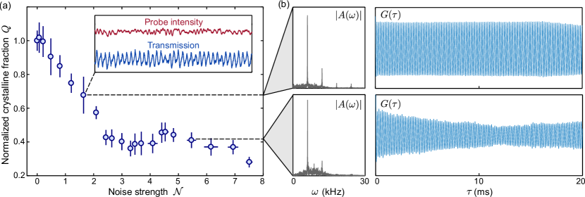
As a defining property, a CTC is predicted to be rigid, i.e., robust against temporal perturbations. To test the rigidity of the observed limit cycle, we add intensity noise on the probe light during the quench dynamics. For a small but finite noise strength , we note that the ordered oscillation of the transmission signal will not suddenly disappear, but preserves the basic pattern found in the noise-free case [see the inset of Fig. 4(a)]. With increasing noise strength, the random noise gradually dominates over the ordered oscillation. To quantify such a melting process of the CTC, we introduce a relative crystalline fraction Kongkhambut et al. (2022), defined as , where and respectively denote the fundamental frequency and the resolution of the DFT amplitude . As shown in Fig. 4(a), the measured crystalline fraction drops almost linearly with the noise strength in the initial stage and then holds within a certain range of strong noise strengths. To investigate the temporal correlation of the melting time crystal, we extract the DFT spectrum and the ACF for measurements performed in different stages [see Fig. 4(b)]. In the linear drop zone, the DFT spectrum still has equally separated spikes embedded in a noisy background. The oscillation of the ACF remains persistent before a slight drop at a very large delay , signaling a preserved LRO. Entering the strong noise region, while the DFT amplitude spectrum has a sharp peak at the fundamental frequency, high-frequency components are erased by the noise. Meanwhile, the noise destroys the LRO, as revealed by the decay of the autocorrelation function for . These observations demonstrate that the long-range temporal correlation can be partially maintained during the melting, confirming that the observed dissipative time crystal is robust to temporal fluctuations of the continuous driving.
In summary, we experimentally demonstrate a dissipative time crystalline order in a room-temperature Rydberg atom ensemble, which is directly observed by the oscillatory transmission of the probe beam. The observed oscillation originates from the simultaneous couplings to distinct Rydberg states, by which the competition between different Rydberg components facilitate the emergence of limit cycles. Importantly, the persistent oscillations has a true long-range temporal order and is robust against noisy perturbations, fulfilling the fundamental criteria of a CTC. By employing a periodic driving, the current setup also holds promise for the study of a discrete time crystal Else et al. (2016); Gong et al. (2018); Lazarides et al. (2020); Cabot et al. (2022); Pal et al. (2018); Cosme et al. (2019); Gambetta et al. (2019); Tuquero et al. (2022). Our work provides a realistic interacting many-body system for systematically investigating the dissipative time crystal, and also opens up a new route to quantum synchronization Khasseh et al. (2019); Buča et al. (2022) and sensing.
Note added. After completion of this work, we became aware of three recent preprints on limit cycles in driven-dissipative systems. In Ref. Greilich et al. (2023), a persistent auto-oscillation is observed in an electron-nuclear spin setup. In Ref. Ding et al. (2023), a transient oscillation induced by inhomogeneous Rydberg excitations is studied. In Ref. Wadenpfuhl and Adams (2023), a synchronized oscillation of Rydberg atoms with different velocities is investigated.
Acknowledgements.
We acknowledge valuable discussions with Klaus Mølmer, Yaofeng Chen, Feng Chen, Yuanjiang Tang, Hadi Yarloo, and Huachen Zhang. This work is supported by the National Key RD Program of China (Grant No. 2018YFA0306504 and No. 2018YFA0306503), the National Natural Science Foundation of China (NSFC) (Grant No. 92265205), and the Innovation Program for Quantum Science and Technology (2021ZD0302100). F. Yang and T. Pohl acknowledge the support from Carlsberg Foundation through the “Semper Ardens” Research Project QCooL and from the Danish National Research Foundation (DNRF) through the Center of Excellence “CCQ” (Grant No. DNRF156).Data availability The data are available from the corresponding author on reasonable request.
Code availability The codes are available upon reasonable request from the corresponding author.
Competing interests The authors declare no competing interests.
References
- Wilczek (2012) F. Wilczek, Phys. Rev. Lett. 109, 160401 (2012).
- Nozières (2013) P. Nozières, Europhys. Lett. 103, 57008 (2013).
- Bruno (2013) P. Bruno, Phys. Rev. Lett. 111, 070402 (2013).
- Watanabe and Oshikawa (2015) H. Watanabe and M. Oshikawa, Phys. Rev. Lett. 114, 251603 (2015).
- Sondhi et al. (1997) S. L. Sondhi, S. Girvin, J. Carini, and D. Shahar, Rev. Mod. Phys. 69, 315 (1997).
- Eisert et al. (2015) J. Eisert, M. Friesdorf, and C. Gogolin, Nat. Phys. 11, 124 (2015).
- Haken (2006) H. Haken, Information and self-organization: A macroscopic approach to complex systems (Springer Science & Business Media, 2006).
- Keßler et al. (2019) H. Keßler, J. G. Cosme, M. Hemmerling, L. Mathey, and A. Hemmerich, Phys. Rev. A 99, 053605 (2019).
- Buča et al. (2019) B. Buča, J. Tindall, and D. Jaksch, Nat. Commun. 10, 1730 (2019).
- Dogra et al. (2019) N. Dogra, M. Landini, K. Kroeger, L. Hruby, T. Donner, and T. Esslinger, Science 366, 1496 (2019).
- Dreon et al. (2022) D. Dreon, A. Baumgärtner, X. Li, S. Hertlein, T. Esslinger, and T. Donner, Nature 608, 494 (2022).
- Shapere and Wilczek (2012) A. Shapere and F. Wilczek, Phys. Rev. Lett. 109, 160402 (2012).
- Sacha and Zakrzewski (2017) K. Sacha and J. Zakrzewski, Rep. Prog. Phys. 81, 016401 (2017).
- Zhang et al. (2017) J. Zhang, P. W. Hess, A. Kyprianidis, P. Becker, A. Lee, J. Smith, G. Pagano, I.-D. Potirniche, A. C. Potter, A. Vishwanath, N. Yao, and C. Monroe, Nature 543, 217 (2017).
- Choi et al. (2017) S. Choi, J. Choi, R. Landig, G. Kucsko, H. Zhou, J. Isoya, F. Jelezko, S. Onoda, H. Sumiya, V. Khemani, C. Keyserlink, N. Yao, E. Demler, and M. Lukin, Nature 543, 221 (2017).
- Rovny et al. (2018) J. Rovny, R. L. Blum, and S. E. Barrett, Phys. Rev. Lett. 120, 180603 (2018).
- Riera-Campeny et al. (2020) A. Riera-Campeny, M. Moreno-Cardoner, and A. Sanpera, Quantum 4, 270 (2020).
- Randall et al. (2021) J. Randall, C. Bradley, F. van der Gronden, A. Galicia, M. Abobeih, M. Markham, D. Twitchen, F. Machado, N. Yao, and T. Taminiau, Science 374, 1474 (2021).
- Kyprianidis et al. (2021) A. Kyprianidis, F. Machado, W. Morong, P. Becker, K. S. Collins, D. V. Else, L. Feng, P. W. Hess, C. Nayak, G. Pagano, N. Yao, and C. Monroe, Science 372, 1192 (2021).
- Keßler et al. (2021) H. Keßler, P. Kongkhambut, C. Georges, L. Mathey, J. G. Cosme, and A. Hemmerich, Phys. Rev. Lett. 127, 043602 (2021).
- Mi et al. (2022) X. Mi, M. Ippoliti, C. Quintana, et al., Nature 601, 531 (2022).
- Taheri et al. (2022) H. Taheri, A. B. Matsko, L. Maleki, and K. Sacha, Nat. Commun. 13, 848 (2022).
- Iemini et al. (2018) F. Iemini, A. Russomanno, J. Keeling, M. Schirò, M. Dalmonte, and R. Fazio, Phys. Rev. Lett. 121, 035301 (2018).
- Bakker et al. (2022) L. Bakker, M. Bahovadinov, D. Kurlov, V. Gritsev, A. K. Fedorov, and D. O. Krimer, Phys. Rev. Lett. 129, 250401 (2022).
- Carollo and Lesanovsky (2022) F. Carollo and I. Lesanovsky, Phys. Rev. A 105, L040202 (2022).
- Krishna et al. (2023) M. Krishna, P. Solanki, M. Hajdušek, and S. Vinjanampathy, Phys. Rev. Lett. 130, 150401 (2023).
- Nie and Zheng (2023) X. Nie and W. Zheng, Phys. Rev. A 107, 033311 (2023).
- Kongkhambut et al. (2022) P. Kongkhambut, J. Skulte, L. Mathey, J. G. Cosme, A. Hemmerich, and H. Keßler, Science 377, 670 (2022).
- Carr et al. (2013) C. Carr, R. Ritter, C. Wade, C. S. Adams, and K. J. Weatherill, Phys. Rev. Lett. 111, 113901 (2013).
- Malossi et al. (2014) N. Malossi, M. Valado, S. Scotto, P. Huillery, P. Pillet, D. Ciampini, E. Arimondo, and O. Morsch, Phys. Rev. Lett. 113, 023006 (2014).
- Ding et al. (2020) D.-S. Ding, H. Busche, B.-S. Shi, G.-C. Guo, and C. S. Adams, Phys. Rev. X 10, 021023 (2020).
- Wu et al. (2021) X. Wu, X. Liang, Y. Tian, F. Yang, C. Chen, Y.-C. Liu, M. K. Tey, and L. You, Chin. Phys. B 30, 020305 (2021).
- Horowicz et al. (2021) Y. Horowicz, O. Katz, O. Raz, and O. Firstenberg, Proc. Natl. Acad. Sci. U.S.A 118, e2106400118 (2021).
- Franz et al. (2022) T. Franz, S. Geier, C. Hainaut, N. Thaicharoen, A. Braemer, M. Gärttner, G. Zürn, and M. Weidemüller, arXiv:2209.08080 (2022).
- Su et al. (2022) H.-J. Su, J.-Y. Liou, I.-C. Lin, and Y.-H. Chen, Opt. Express 30, 1499 (2022).
- Medenjak et al. (2020) M. Medenjak, B. Buča, and D. Jaksch, Phys. Rev. B 102, 041117 (2020).
- Guo and You (2022) T.-C. Guo and L. You, Frontiers in Physics 10 (2022).
- Greilich et al. (2023) A. Greilich, N. Kopteva, A. Kamenskii, P. Sokolov, V. Korenev, and M. Bayer, arXiv:2303.15989 (2023).
- Else et al. (2016) D. V. Else, B. Bauer, and C. Nayak, Phys. Rev. Lett. 117, 090402 (2016).
- Gong et al. (2018) Z. Gong, R. Hamazaki, and M. Ueda, Phys. Rev. Lett. 120, 040404 (2018).
- Lazarides et al. (2020) A. Lazarides, S. Roy, F. Piazza, and R. Moessner, Phys. Rev. Research 2, 022002 (2020).
- Cabot et al. (2022) A. Cabot, F. Carollo, and I. Lesanovsky, Phys. Rev. B 106, 134311 (2022).
- Pal et al. (2018) S. Pal, N. Nishad, T. Mahesh, and G. Sreejith, Phys. Rev. Lett. 120, 180602 (2018).
- Cosme et al. (2019) J. G. Cosme, J. Skulte, and L. Mathey, Phys. Rev. A 100, 053615 (2019).
- Gambetta et al. (2019) F. Gambetta, F. Carollo, M. Marcuzzi, J. Garrahan, and I. Lesanovsky, Phys. Rev. Lett. 122, 015701 (2019).
- Tuquero et al. (2022) R. J. L. Tuquero, J. Skulte, L. Mathey, and J. G. Cosme, Phys. Rev. A 105, 043311 (2022).
- Khasseh et al. (2019) R. Khasseh, R. Fazio, S. Ruffo, and A. Russomanno, Phys. Rev. Lett. 123, 184301 (2019).
- Buča et al. (2022) B. Buča, C. Booker, and D. Jaksch, SciPost Phys. 12, 097 (2022).
- Ding et al. (2023) D.-S. Ding, Z. Bai, Z.-K. Liu, B.-S. Shi, G.-C. Guo, W. Li, and C. S. Adams, arXiv:2305.07032 (2023).
- Wadenpfuhl and Adams (2023) K. Wadenpfuhl and C. S. Adams, arXiv:2306.05188 (2023).
- Lee et al. (2011) T. E. Lee, H. Häffner, and M. Cross, Phys. Rev. A 84, 031402 (2011).
- Qian et al. (2012) J. Qian, G. Dong, L. Zhou, and W. Zhang, Phys. Rev. A 85, 065401 (2012).
- Šibalić et al. (2016) N. Šibalić, C. G. Wade, C. S. Adams, K. J. Weatherill, and T. Pohl, Phys. Rev. A 94, 011401 (2016).
- He et al. (2022) Y. He, Z. Bai, Y. Jiao, J. Zhao, and W. Li, Phys. Rev. A 106, 063319 (2022).
- Marcuzzi et al. (2014) M. Marcuzzi, E. Levi, S. Diehl, J. P. Garrahan, and I. Lesanovsky, Phys. Rev. Lett. 113, 210401 (2014).
- Strogatz (2018) S. H. Strogatz, Nonlinear dynamics and chaos with student solutions manual: With applications to physics, biology, chemistry, and engineering (CRC press, 2018).
- Miller et al. (2016) S. A. Miller, D. A. Anderson, and G. Raithel, New J. Phys. 18, 053017 (2016).
- Ripka et al. (2018) F. Ripka, H. Kübler, R. Löw, and T. Pfau, Science 362, 446 (2018).
- Li et al. (2022) W. Li, J. Du, M. Lam, and W. Li, Opt. Lett. 47, 4399 (2022).
Methods
Mean-field description of the dynamics
As our experiments are carried out with a large intermediate state detuning , the resulting dynamics can be reasonably described by the V-type three-level model shown in Fig. 1(d). Then, the time translation invariant Hamiltonian (in the rotating frame) of the model is given by
| (1) |
where is the atomic transition operator (), and () denotes the local Rydberg density. Here, we assume an equal interaction strength for different Rydberg levels and . Taking the Rydberg decay into consideration, the evolution of an operator is governed by
| (2) |
where is the Lindbladian describing the decay of the Rydberg state (). The equations of motion for the first moments are then determined by
In the mean-field treatment Lee et al. (2011); Qian et al. (2012); Šibalić et al. (2016); He et al. (2022), we neglect the correlation between different atoms, which allows for a factorization of the high-order moments, e.g., . Assuming a uniform spatial distribution Marcuzzi et al. (2014), e.g., , we arrive at the mean-field equations:
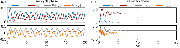
where is the nonlinear energy shift with . The stable behavior of the system is determined by the property of the fixed points of the above nonlinear Bloch equations. With a standard stability analysis Strogatz (2018), we can analyze types of bifurcations and obtain the phase diagram shown in Fig. 1(d), where we set and . In Fig. 5, we calculate the mean-field dynamics in different regimes. When the system is in the limit cycle phase, the mean-field components exhibit persistent periodic oscillations after an initial synchronization [see Fig. 5(a)]. Here, oscillation of the imaginary part of the transition dipole causes an oscillating absorption coefficient of the probe field, which can be directly monitored by the transmission signal as in our experiment. Instead, if the system is in the stationary phase [see Fig. 5(b)], all observables will eventually converge to their steady-state values.
Experimental details
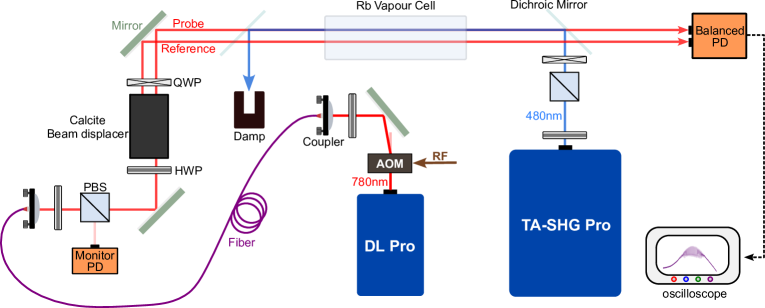
The detailed experimental setup is depicted in Fig. 6. Our experiments are performed in a 7.5-cm-long room-temperature Rb vapour cell Miller et al. (2016); Ripka et al. (2018); Li et al. (2022) with natural abundance, where the proportions of 85Rb and 87Rb isotopes are about 72.2% and 27.8%. The laser sources of 780-nm and 480-nm light fields are [Toptica DL pro @780nm] and [Toptica TA-SHG pro @480nm], and both of them can work in the frequency-scanning mode or the frequency-locking mode. For 780-nm laser, we use an acoustic optical modulator (AOM) before the coupler of the fiber to control the output laser intensity, which is monitored by an independent PD. Then, a calcite beam displacer (Thorlabs BD40) is used to generate two parallell 780-nm beams for differential measurements, one of which is chosen as the probe beam (overlapped with a 480-nm coupling beam) with the other being a reference. The maximum powers of the probe ( waist radius ) and the coupling ( waist radius ) beams are approximately and , with which the maximum Rabi frequencies are approximately and (dependent on the laser polarization and the specific Zeeman level). The transmission spectrum is obtained by scanning the frequency of the coupling field (the detuning ) at a fixed intermediate-state detuning around the two-photon resonance .
For the measurement of the quench dynamics, the frequencies of both laser sources are locked to an ultralow expansion (ULE) cavity with the help of the Pound-Drever-Hall (PDH) technique. Then, by controlling the radio frequency (RF) driving on the AOM, we can turn on and off the 780-nm output laser abruptly within s, during which the 480-nm laser is always kept on. When exploring the rigidity of the dissipative time crystal, the intensity noise added to the probe field is achieved by using a waveform generator (Keysight 33600A Series) to modulate the RF amplitude.
To adjust the energy spacing of different Rydberg Zeeman sublevels, we use a homemade 7.5-cm-long coil with 35 windings to generate a homogeneous external magnetic field parallel to the laser beams. Meanwhile, quarter-wave plates (QWP) are used to control the polarizations of the 780-nm and 480-nm light fields, with which we can tune the coupling strengths to different Zeeman levels (see Fig. 2 of the main text).
While the data shown in this paper is based on the excitation of 85Rb isotopes, similar oscillatory behavior is also observed for 87Rb isotopes, indicating that the oscillating dynamics is a universal phenomenon in Rydberg atomic ensembles. However, the appearance of the limit cycle phase for 87Rb atoms is rarer than 85Rb atoms, which can be attributed to the lower natural abundance of 87Rb isotopes and can be improved by increasing the atomic density with an additional heating.
Influence of the principal quantum number
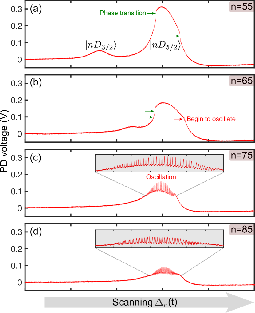
It is necessary to exicite atoms to a high principal quantum number for the observation of oscillatory signals. Figure 7(a)-(d) show the transmission spectrum at different , where the probe (coupling) beam is elliptically (linearly) polarized with no external magnetic field. At a relatively small , as expected, there are only two distinct transmission peaks, representing the resonant positions or energy levels of two Rydberg -state manifolds with total angular momentum quantum numbers and . The peak of the latter is higher due to the larger dipole matrix element between the Rydberg state and the intermediate state. In other words, the Rabi frequency of coupling beam for is larger than . Consequently, the Rydberg population is also higher for , leading to non-equilibrium dynamical phase transitions in bistable regions where the signal abruptly changes (green arrows).
When is increased to 65 [see Fig. 7(b)], the overall peaks become lower due to the smaller coupling Rabi frequency which scales as . The energy difference between two Rydberg states also becomes smaller. Here, multiple phase transitions in the left side of are identified, and the emergent oscillatory signal appears in the right side of (red arrow). Dramatic changes to the above features occur when is further increased [see Fig. 7(c)-(d)]. As and become closer, the two Rydberg states came to merge and the oscillation signal gets amplified over a wide range of the detuning . In general, the appearance and the enhancement of the oscillating dynamics with an increasing can be attributed to: (i) the stronger Rydberg interactions, and (ii) the participation of more Rydberg states (within and manifold) in the dynamics.
Long-term stability of the oscillation frequency
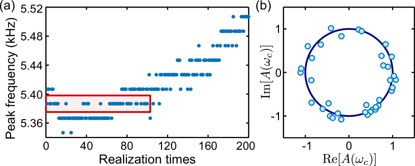
As described in the main text, the oscillating signal will synchronize to a stable frequency in each single shot realization of the quench dynamics. However, two independent realizations separated by a very long time can still possess very different stable frequencies, due to the drift of experimental conditions, e.g., room temperatures and magnetic noises. For the measurement performed in Fig. 3(c), we record 200 independent realizations of the quench dynamics, which are separated into 50 groups, with a 125 ms duration between successive realizations within each group and a 10 s duration between nearest groups. As shown in Fig. 8(a), the extracted peak frequencies of the DFT spectrum (performed for the time window 50-100 ms, already in the stable periodic region) for these 200 realizations have a long-term drift, approximately 6 times of the DFT resolution. To control the influence of frequency drifts, we select the first 100 realizations for Fig. 4(c). The evolution of the peak frequency obeys the same law if we choose the full 200 realizations, albeit with a slightly larger error bar.
Here, we also show that the aperiodic to periodic transition can naturally induce a random phase distribution of the established time crystal. To avoid the phase uncertainty caused by fluctuations of the oscillation frequency, we further postselect the data of the same frequency from the first 100 realizations (indicated by the red box in Fig. 8(a). As shown in Fig. 8(b), the phase of the Fourier amplitude at the peak frequency is randomly distributed over , indicative of a spontaneous time translation symmetry breaking.