Rare Life Event Detection via Mobile Sensing Using Multi-Task Learning

Abstract

Rare life events significantly impact mental health, and their detection in behavioral studies is a crucial step towards health-based interventions. We envision that mobile sensing data can be used to detect these anomalies. However, the human-centered nature of the problem, combined with the infrequency and uniqueness of these events makes it challenging for unsupervised machine learning methods. In this paper, we first investigate granger-causality between life events and human behavior using sensing data. Next, we propose a multi-task framework with an unsupervised autoencoder to capture irregular behavior, and an auxiliary sequence predictor that identifies transitions in workplace performance to contextualize events. We perform experiments using data from a mobile sensing study comprising N=126 information workers from multiple industries, spanning 10106 days with 198 rare events ($<2\%$). Through personalized inference, we detect the exact day of a rare event with an F1 of 0.34, demonstrating that our method outperforms several baselines. Finally, we discuss the implications of our work from the context of real-world deployment.

Data and Code Availability.

Tesserae study data (Mattingly et al., 2019) can be obtained through a data usage agreement (https://tesserae.nd.edu/). Code is not publicly available, but provided on request.

Institutional Review Board (IRB).

The study protocol is fully approved by the Institutional Review Boards at Dartmouth College, University of Notre Dame, University of California-Irvine, Georgia Tech, Carnegie Mellon University, University of Colorado-Boulder, University of Washington, University of Texas-Austin, and Ohio State University. This research is based upon work supported in part by the Office of the Director of National Intelligence (ODNI), Intelligence Advanced Research Projects Activity (IARPA), via IARPA Contract No. 2017-17042800007. The views and conclusions contained herein are those of the authors and should not be interpreted as necessarily representing the official policies, either expressed or implied, of ODNI, IARPA, or the U.S. Government.

1 Introduction

Life events (LE) are significant changes in an individual’s circumstances that affect interpersonal relationships, work, and leisure (Hill, 2002). The nature of these events inevitably affect mental well-being and general health (Goodyer, 2001). The detrimental effects of adverse LEs (e.g., death of a loved one, losing a job, terminal illness) have been widely studied and known to be associated with a higher incidence of depression and altered brain network structure (Falkingham et al., 2020; Gupta et al., 2017). In contrast, positive LEs (e.g., taking a vacation, job promotion, childbirth) are associated with increased life satisfaction, and higher cognitive function (Castanho et al., 2021). Moreover, LEs affect cardiovascular vascular disease risk factors, such as increased central adiposity, heightened exposure to inflammation, and elevated resting blood pressure (Steptoe and Kivimäki, 2013). A study by Steptoe and Kivimäki (2012) suggests that even minor LEs can trigger cardiac events like myocardial ischemia.

Sensing data is a multivariate time series, and traditional ML approaches for anomaly detection include the One-Class SVM (OCSVM) (Ma and Perkins, 2003), Isolation Forest (IF) (Liu et al., 2008), and logistic regression (Hilbe, 2009). However, these approaches do not capture temporal dependencies. Additionally, creating user-specific thresholds is critical in human-centered tasks. Thus, methods which directly predict anomalies (IF) or require threshold parameter tuning (OCSVM) are not ideal.

Recently, timeseries based autoencoders have received significant attention (Rumelhart et al., 1985; Zhou and Paffenroth, 2017; Audibert et al., 2020; Su et al., 2019), and many methods use RNN variants such as LSTM (Hochreiter and Schmidhuber, 1997) and GRU (Cho et al., 2014) to capture temporal dependencies. In an autoencoder, the reconstruction error is used to detect anomalies. However, the complexity of human behavior and class imbalance creates biased learned representations, making it challenging to distinguish normal and rare events (Pang et al., 2021). An intuitive solution to this problem involves increasing the error of rare events without affecting normal events. Multi-task learning achieves this by incorporating additional information from a related task(s) to learn a shared representation, and thus compensate for the limitations of a purely unsupervised approach (Sadhu et al., 2019; Wu et al., 2021).

In this paper, we first use statistical analysis to examine whether LEs result in behavioral shifts observable through mobile sensing. Next, we propose Multi-Task Anomaly Detection (MTAD) to detect “in-the-wild” rare LEs using behavioral mobile sensing data. We hypothesize that a standalone unsupervised autoencoder cannot effectively capture differences between normal and rare events using the reconstruction error because of the heterogeneity in human data and the significant class imbalance ($<2\%$ rare events). Thus, MTAD trains an auxiliary sequence predictor to contextualize events by capturing changes in workplace performance due to the event. For example, a participant reported that getting promoted positively impacted their work performance, while another person mentioned that visiting their sick parents had a negative effect. We aim to identify such changes at inference and compute a scaling factor that magnifies the reconstruction error of rare events.

1.1 Contributions

Toward the vision of detecting life events from mobile sensing data collected in in-the-wild settings, our main contributions are as follows. First, we perform granger-causality testing to detect if the days before an event can be used to predict days after the event. Thus, establishing a relationship between LEs and behavior (section 4). Second, we propose a multi-task learning architecture consisting of two components: (1) an LSTM based encoder-decoder to calculate an anomaly score, and (2) a sequence predictor to contextualize the anomaly score by inferring a transition in workplace performance (section 5). Third, we perform empirical analysis on a real-world dataset to compare MTAD with five state-of-the-art baselines to analyze performance and robustness (section 5.4). Finally, we rigorously evaluate parameters that affect MTAD (section 5.4) and discuss implications of our research (section 6).

2 Related Work

2.1 Change Point Detection

Change point detection (CPD) refers to the change in the state of a time series. CPD has been applied to various physiological signals (Shvetsov et al., 2020; Fotoohinasab et al., 2020; Stival et al., 2022). For example, Shvetsov et al. (2020) propose an unsupervised approach based on point clouds and Wasserstein distances to detect six different types of arrhythmias. Designing appropriate metrics that can identify change is vital in CPD. Consequently, Chen et al. (2019) design a metric for EEG CPD by modifying several similarity metrics from other domains. In fitness, Stival et al. (2022) propose a method combining CPD and Gaussian state space models to detect actionable information such as physical discomfort and de-training.

2.2 Anomaly detection methods

Approaches for anomaly detection in multivariate time series are varying, and several challenges exist based on the method, and applied area (Pang et al., 2021). In deep learning, the LSTM encoder-decoder (or LSTM autoencoder) has received a lot of attention. Malhotra et al. (2016) demonstrate the robustness of using an LSTM in an autoencoder framework. Similarly, Park et al. (2018) propose the LSTM-VAE, which combines the temporal modeling strength of LSTM with the variational inference capability of a VAE. The resulting model obtains better generalization for multimodal sensory signals. The Deep Autoencoding Gaussian Mixture Model (DAGMM) jointly optimizes two components to enable optimal anomaly detection, an autoencoder computes a low-dimensional representation, and a gaussian mixture model that predicts sample membership from the compressed data (Zong et al., 2018). Audibert et al. (2020) propose an adversarially trained autoencoder framework to detect anomalies. For anomalous driving detection, Sadhu et al. (2019) introduce a multi-task architecture that magnifies rare maneuvers using domain knowledge regarding the frequency of driving actions.

2.3 Life event detection

To the best of our knowledge, there are two works similar to ours. First, Faust et al. (2021) use OCSVM to assess the response to an adverse life event using physiological and behavioral signals from wrist-worn wearables. They focus on examining the responses to the adverse event and the coping strategies employed by the participant. Their findings suggest the existence of behavioral deviations after a negative event, motivating us to focus on prediction. Second, Burghardt et al. (2021) detect abnormal LEs using wrist-worn wearables from hospital and aerospace workers. Their method works by first creating a time series embedding using a hidden markov model variant and then uses a random forest or logistic regression for classification.

Our work differs from the previous studies in several ways: (1) we use smartphone behavioral data instead of wearable physiological data, (2) we consider postive, negative, and multiple LEs (differing from Faust et al. (2021)), (3) we focus on deep models instead of traditional ML, (4) our data has an extremely low anomaly ratio ($<2\%$) compared to Burghardt et al. (2021) (11.7% and 14.9%). Thus, we view our problem to be significantly challenging. Moreover, we provide crucial statistical motivation to pursue LE detection.

3 Study

The Tesserae study (Mattingly et al., 2019) recruited 757 information workers across different companies in the USA for one year where participants respond to several surveys. They were instrumented with a Garmin vivoSmart 3 wearable and a continuous sensing app is installed on their phone. Participants are instructed to maintain data compliance level of 80% to warrant eligibility for monetary remuneration. The sub-cohort’s age ranged from 21 to 64, with an average of 34. Of the 126 individuals, the dataset is fairly balanced with 67 and 59 identified as male and female, respectively. The top 3 areas of occupation were Computer and Mathematical Sciences, Business and Finance, and Engineering. Roughly 98% of the participants had at least a college degree. In terms of mobile platform, the cohort had 66 Android users and 60 iOS users. Please refer to the link in the data availability statement to learn about the Tesserae study. Additional demographic information is listed in Appendix A.3.

3.1 Features

In contrast to studies using wearable physiology data (Faust et al., 2021; Burghardt et al., 2021), we use daily summaries of behavioral mobile sensing features in our analyses. Overall, we used walking duration, sedentary duration, running duration, distance traveled, phone unlock duration, number of phone unlocks, number of locations visited, and number of unique locations visited. Further, to better understand user behavior, we divide the features (except number of unique locations visited) into 4 “epochs” for modelling: epoch 1 (12am - 6am), epoch 2 (6am - 12pm), epoch 3 (12pm - 6pm), and epoch 4 (6pm - 12am). Ultimately, 29 features were used for analyses. Previous studies elucidate the importance of these features to understand human behavior from a workplace context (Nepal et al., 2020; Mirjafari et al., 2019).

3.2 Ground Truth

The definition of a significant life event is subjective and depends on the individual. We adopt a widely accepted definition from job stress literature, which describes these events as situations where psychological demand exceeds available resources (Karasek et al., 1981).

After study completion, participants were asked to describe significant LEs using their diaries, calendars, and other documents. Participants provided free-text descriptions for every event, start and end dates, date confidence, significance, valence (positive/negative), type of event, and workplace performance impact. Valence, date confidence, and workplace performance are reported on a 1-7 likert scale as follows: (1) Valence: “1” indicated “Extremely Positive” and “7” indicated “Extremely Negative”, and (2) Date confidence: “1” indicated “Lowest confidence” and “7” indicated “Highest confidence”. Workplace performance impact is assigned to one of the following - “Large Negative Effect”, “Medium Negative Effect”, “Small Negative Effect”, “No Effect”, “Small Positive Effect”, “Medium Positive Effect”, “Large Positive Effect”.

Our selection criteria is as follows: (1) Valence must be Extremely Positive, Very Positive, Very Negative, or Extremely Negative, and (2) Date confidence must be “Moderately High”, “High”, or “Highest”. Next, we set a 30-day date limit before and after an event for analysis. For overlapping events, the limit is set 30 days before and after the first and last events, respectively. These choices are based on a study by Faust et al. (2021) examining the impact of LEs within a 60-day period. Finally, the missingness and uneven spacing (discontinuous days) within this time frame must be $<25\%$. Every day was labelled as “1” indicating a rare event or “0” indicating a normal event. For workplace performance, the label is forward filled, and an “Unknown” label is assigned to days before the rare event. Our final dataset consists of 10106 days from 126 participants with 198 rare LEs ($<2\%$).

4 Statistical Testing

Initially, we ask the question: “Does the behavior of an individual change after an LE?”. If so, what features are significant in most of the time series? To this end, we applied the granger-causality test as follows. First, we split the 159 multivariate time series (29 features) into two parts, one before and including the rare event ($T^{pre}$) and the other after the rare event ($T^{post}$). Next, for each feature, a granger-cause test is applied to investigate if $T^{pre}$ granger-causes $T^{post}$. A $p<0.05$ implies the time series for the specific feature is significant. Finally, we sum the significant time series across each feature. For example, in Figure 1, loc_visit_num_ep_1 has a value of 42, which implies that 42 out of 159 time series were granger-cause significant. We used the statsmodel package for python to apply the granger-cause test with a lag of upto 6. The SSR-based F-test is used to evaluate statistical significance at $p=0.05$. Significance at any lag is considered granger-causality, and the total number of significant time series (out of 159) for each feature is displayed in Figure 1.

From Figure 1, we observe that the number of locations visited and location distance between 12am-6am and 12pm-6pm is significantly impacted by LEs in several cases, suggesting location behaviors are crucial to LE detection. In addition, we observe that walking and running have approximately the same number of granger-cause time series across episodes, suggesting an overall change throughout the day rather than a shift in the timing of these activities. In contrast, sedentary action varies across episodes, suggesting that LEs might affect the sedentary state at different times of the day. Also, unlock duration and count vary due to a life event. While the number of unlocks between 12am-6am has the most number of significant time series, the unlock duration between 6am-12pm has more significance comparatively.

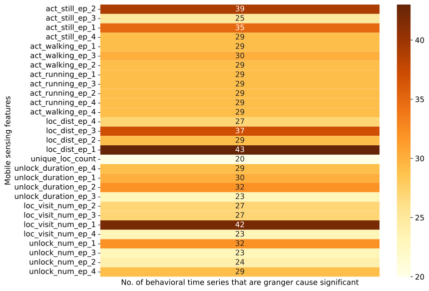
Figure 1: Heatmap indicating the number of time series (out of 159) that are granger-cause significant at $p<0.05$. Larger values imply that the corresponding feature changes after an LE in many participants, and could be important for detection. The x-axis is the number of significant time series, i.e., the count of significant time series out of 159. The y-axis are the mobile sensing features. “act” is an activity which can be still, walking, running. “loc” specifies location. “dist” is distance. “num” is number.

5 Multi-task anomaly detection

5.1 Problem formulation

Given a set of $I$ participants, we define a multivariate time series for each user $u\in\{1,\ldots,I\}$ with $T$ days as $\mathcal{T}^{u}=\{{\boldsymbol{x}^{u}_{1}},\ldots,\boldsymbol{x}^{u}_{T}\}$, where $\boldsymbol{x}\in\mathbb{R}^{m}$ , $m$ is the number of mobile sensing features, and $t\in\{1,\ldots,T\}$ is a specific day. To model temporal dependencies, we apply a rolling window approach to the time series. A window at day $t$ with a predefined length $l$ is given by:

$$W_{t}=\{\boldsymbol{x}_{t-l+1},\ldots,\boldsymbol{x}_{t-1},\boldsymbol{x}_{t}\}$$ (1)

Using equation (1), the user’s multivariate time series $\mathcal{T}^{u}$ is transformed into a collection of windows $\mathcal{W}=\{W_{1},\dots,W_{T}\}$, where $W\in\mathbb{R}^{l\times m}$. Next, a window is assigned a binary label $y^{R}\in\{0,1\}$, where $y^{R}=1$ indicates a rare life event at the time $t$ (i.e., $y_{t}^{R}=1$) and $y^{R}=0$ indicates a normal event in all other cases. Observe that we only consider the exact day of the rare event to be a rare window. Given that each participant’s windows is transformed separately, we generalize the entire collection of normal and rare event windows across participants as $\mathcal{W}_{normal}=\{W_{1},\ldots,W_{N}\}$ and $\mathcal{W}_{rare}=\{W_{1},\dots,W_{R}\}$, respectively.

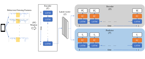
Figure 2: The proposed multi-task learning architecture illustrating training information flow for a window $W$ of length $l$.

In our context, we define a multi-task model with two related tasks trained using $\mathcal{W}_{normal}$. First, an unsupervised learning task trained to reconstruct the input $\mathcal{W}_{normal}$, which produces higher errors or anomaly scores when reconstructing $\mathcal{W}_{rare}$. Thus, facilitating rare life event detection. Second, a supervised learning task to contextualize and scale the anomaly score. Here, $\mathcal{W}_{normal}$ is trained to predict a workplace performance vector $\boldsymbol{y}\in\mathbb{R}^{l}$, where each day $t\in\{1,\ldots,l\}$ in $W$ represented by $y_{t}$ belongs to one of the workplace performance labels described in 3.2.

Problem Statement. Given a participant’s multivariate time series window $W_{t}$ and the corresponding workplace performance vector $\boldsymbol{y}$, the objective of our problem is to train a multi-task framework capable of detecting a rare life event at time $t$.

5.2 Multi-task Architecture

Our multi-task framework (Figure 2) consists of three components: an encoder E which maps a window $W$ to a low-dimensional representation (latent space) $Z$, a decoder $D$ to reconstruct $W$ from $Z$ (5.2.1), and a sequence predictor $P$ to predict the workplace performance vector $\boldsymbol{y}$ (5.2.2).

5.2.1 Unsupervised Autoencoder (Task A)

We capture temporal dependencies from the multivariate time series using LSTMs (Hochreiter and Schmidhuber, 1997) to build the encoder-decoder architecture. An LSTM encoder learns from an input window $W$ by running through the day-wise input sequence and computes a fixed size latent space $Z$. Next, $Z$ is copied multiple times to match the length of the window. Finally, the LSTM decoder $D$ uses $Z$ to reconstruct the input sequence, and the reconstructed sequence is represented as $\overline{W}$. We train the LSTM encoder-decoder (LSTM-ED) by minimizing the reconstruction error between $W$ and $\overline{W}$ using the mean squared error defined as:

$$\mathcal{L}_{A}=\frac{1}{l\times m}\|W-\overline{W}\|^{2}_{F}$$ (2)

where $\overline{W}=D(Z)$; $Z=E(W)$; $\|\cdot\|_{F}$ is the Frobenius norm

Recall that we only use $\mathcal{W}_{normal}$ to train the LSTM-ED to learn normal event representations. Therefore, by using the reconstruction error as an anomaly score $\alpha$, we can detect rare events based on their higher $\alpha$ values. However, it is possible that some participants or events do not exhibit significant behavior changes which can be captured by our LSTM-ED through $\alpha$. To address this challenge, we attempt to identify anomalies through a supervised learning setup in the next section. Srivastava et al. (2015) describes LSTM encoder-decoder architectures in detail.

Input: $\mathcal{D}_{train}$ with $\mathcal{W}_{normal}=\{W_{1},\ldots,W_{N}\}$, $\{Y_{1},\ldots,Y_{N}\}$, class weight vector $\boldsymbol{w}$, and number of epochs $E$.

Output: Trained $E$, $D$, $P$

$E$, $D$, $P$ $\leftarrow$ initialize weights;

$e\leftarrow 1$;

repeat

       for $n\leftarrow 1$ to $N$ do

             $Z_{n}\leftarrow E(W_{n})$;

             $\overline{W_{n}}\leftarrow D(Z_{n})$;

             $\widehat{Y_{n}}\leftarrow P(Z_{n})$;

             $\mathcal{L}_{A}\leftarrow\frac{1}{l\times m}\|W_{n}-\overline{W_{n}}\|^{2}_{F}$;

             $\mathcal{L}_{B}\leftarrow-\sum_{i=1}^{l}\sum_{j=1}^{c}Y_{nij}\times\ln(\widehat{Y_{nij}})\times w_{j}$;

             $\mathcal{L}\leftarrow\mathcal{L}_{A}+\mathcal{L}_{B}$;

             $E,D,P\leftarrow$ update weights using $\mathcal{L}$;

            

       end for

      $e\leftarrow e+1$;

      

until $e=E$;

Algorithm 1 Training

5.2.2 Sequence Prediction (Task B)

To scale the anomaly score $\alpha$, we train a supervised sequence predictor $P$ to detect day-wise workplace performance. The window $W$ and a true workplace performance label vector $\boldsymbol{y}\in\mathbb{R}^{l}$ as training inputs, where the label for day $t\in\{1,\ldots,l\}$ in $W$represented by $y_{t}$ has one of the performance labels described in section 3.2. Moreover, $Y\in\mathbb{R}^{l\times c}$ represents one-hot vectors from $\boldsymbol{y}$ with $c$ classes ($c$ = 8). Observe that $W$ is same for tasks A and B. Hence, our architecture shares the LSTM encoder network $E$ described in section 5.2.1. For Task B, $P$ is composed of an LSTM network to further extract temporal features from the latent representation $Z$ followed by a fully connected layer $FC$ (softmax activation) to predict day-wise class probabilities ${\widehat{Y}}$. At inference, ${\widehat{Y}}$ is mapped to the predicted workplace performance label vector $\boldsymbol{\widehat{y}}$. The model is optimized using the weighted categorical cross-entropy loss function defined by:

$$\mathcal{L}_{B}=-\sum_{i=1}^{l}\sum_{j=1}^{c}Y_{ij}\times\ln(\widehat{Y_{ij}})\times{w_{j}}$$ (3)

where $\widehat{Y}=\text{softmax}(FC)$; $w_{j}\text{ is the weight for class }j$.

From equations (2) and (3), we can represent the final loss function as $\mathcal{L}=\mathcal{L}_{A}+\mathcal{L}_{B}$. The proposed multi-task architecture is trained in an end-to-end fashion, where the tasks A and B are jointly optimized by minimizing $\mathcal{L}$ (Algorithm 1).

5.2.3 Inference

The detection phase workflow (Algorithm 2) computes the anomaly score $\alpha$ from Task A and a scaling factor $s$ from Task B for each test window.
Anomaly Score. Recall that, our goal is to identify a rare event on the exact day. Thus, we unroll $W$ and $\overline{W}$ to compute the score for the most recent day $t$ as follows:

$$\alpha=\frac{1}{m}\sum_{j=1}^{m}(x_{j}-\overline{x_{j}})^{2}$$ (4)

where $\boldsymbol{x}\text{ and }\boldsymbol{\overline{x}}$ are the true and reconstructed multivariate time series, respectively; $m$ is the number of mobile sensing features.
Scaling factor. The effect of stressful life events affect work-life balance in US workers and reduce productivity (Hobson et al., 2001). Thus, there is reason to believe workplace performance shifts after an LE. To capture this change, we first transform the predicted workplace performance vector $\boldsymbol{\widehat{y}}$ into a binary vector $\boldsymbol{r}\in\mathbb{R}^{l-1}$ defined as:

$$r_{t-1}=\begin{cases}1&\widehat{y}_{t}\neq\widehat{y}_{t-1}\\ 0&otherwise\\ \end{cases}$$

where $t\in\{2,\ldots,l\}$

In essence, we identify the day of workplace performance change and use it as a proxy for rare event detection. For example, consider a $\boldsymbol{\widehat{y}}=$ [“Unknown”, “Unknown”, “Large Negative Effect”] with $l=3$, then the transition vector is $r=[0,1]$. Initially, we assumed that a value “1” on the most recent day could be directly used to detect the rare event. However, this idea had two major limitations. First, it is possible that larger window sizes might have multiple transitions ($r_{t}=1$). Second, erroneous predictions might hinder detection. Thus, we exponential weight our transition vector $r$. Intuitively, more recent workplace performance shifts have larger impact on behavioral changes owing to LE. The scaling factor $s$ aims to capture the abovementioned effect as follows:

$$s=\frac{1}{l-1}\sum_{t=1}^{l-1}e^{-\lambda tr_{t}}$$ (5)

where $\lambda$ is a constant decay factor.

Detection. The final scaled anomaly score $\delta$ is computed from equations (4) and (5) in the following way: $\delta=\frac{\alpha}{s}$. Observe that $\delta=\alpha$ when $\boldsymbol{r}$ is a zero vector, i.e., a vector with no workplace performance changes. Ultimately, a window $W_{t}$ with a scaled anomaly score $\delta$ has a rare life event at $t$ ($y^{R}_{t}=1$) if $\delta$ is greater than a threshold $\gamma$. However, the scarcity of rare events hindered threshold tuning based on performance metrics. Thus, $\gamma$ is the 95^th percentile anomaly scores from the validation data set.

Input: $\mathcal{D}_{test}$ with $\mathcal{W}=\{W_{1},\ldots,W_{N+R}\}$, $\gamma$ from $D_{val}$, $l$, $\lambda$.

Output: $\boldsymbol{y^{R}}=\{y^{R}_{1},\ldots,y^{R}_{N+R}\}$

for $n\leftarrow 0$ to $N+R$ do

       $Z_{n}\leftarrow E(W_{n})$;

       $\overline{W_{n}}\leftarrow D(Z_{n})$;

       $\widehat{Y_{n}}\leftarrow P(Z_{n})$;

       $\boldsymbol{x},\overline{\boldsymbol{x}}\leftarrow$ unroll($W_{n}$), unroll($\overline{W_{n}}$) ;

       $\alpha\leftarrow\frac{1}{m}\sum_{j=1}^{m}(x_{j}-\overline{x_{j}})^{2}$;

       $\widehat{\boldsymbol{y}}\leftarrow$ get class labels from probabilities $\widehat{Y_{n}}$;

       $\boldsymbol{r}\leftarrow$ compute binary transition vector from $\widehat{\boldsymbol{y}}$;

       $s\leftarrow\frac{1}{l-1}\sum_{t=1}^{l-1}e^{-\lambda tr_{t}}$;

       $\delta\leftarrow\frac{\alpha}{s}$;

       if $\delta>\gamma$ then

             $y^{R}_{n}\leftarrow 1$;

            

      else

            $y^{R}_{n}\leftarrow 0$;

       end if

      

end for

Algorithm 2 Inference

5.3 Experimental Setup

We performed several pre-processing steps for optimal training and inference. First, we impute missing data and unevenly sampled time series using the mean. Second, we forward fill missing rare event and workplace performance labels. Third, within-subject feature normalization is applied as a precursor for personalization. Finally, each participant’s time series is transformed into windows of length $l=10$ using equation (1).

In our analysis, we divide $\mathcal{W}_{normal}$ and the corresponding $y$ into training ($\mathcal{D}_{train}$), validation ($\mathcal{D}_{val}$), and test ($\mathcal{D}_{test}$) with ratio of 80:10:10, respectively. Next, we append $\mathcal{W}_{rare}$ to $\mathcal{D}_{test}$. Note that rare events are held-out for testing and are neither used for training nor validation. Moreover, we generate ten different user-dependent splits to ensure the training, validation, and test data sets consist of time series from all participants. To assess positive class performance in imbalanced data, we use precision (P), recall (R), and the F1-score, and report mean and standard deviation across the splits. The windows are unrolled at inference to detect a rare event on the exact day. Thus, identifying if a rare event is present within a window is not considered to be an accurate detection.

5.4 Results

In this section, we examine the properties of the proposed framework by comparing it with other baselines (5.4.1), analyzing the strengths of personalization (5.4.2), and estimating the changes in performance at different window sizes and decay constants for the scaling factor (5.4.3). Next, we perform an ablation study to assess the necessity of the sequence predictor (5.4.4). Finally, we assess the types of events identified by MTAD (5.4.5).

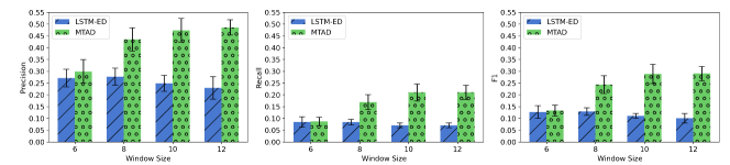
Figure 3: Comparison between general LSTM-ED and MTAD at different window sizes.

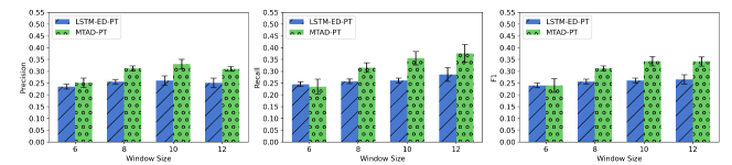
Figure 4: Comparison between LSTM-ED-PT and MTAD-PT at different window sizes.

5.4.1 Performance

We evaluate the performance of our algorithm by comparing it with five state-of-the-art baselines for anomaly detection, namely, OCSVM, IF, LSTM-VAE, DAGMM, and LSTM-ED. As shown in Table 1, MTAD performs significantly better than all traditional machine learning and deep learning methods in terms of P, R, and F1. Particularly, MTAD’s 0.29 F1 score is 2.6 times greater than a standard LSTM autoencoder (LSTM-ED). Unlike other methods, DAGMM does not compute a normal event decision boundary, i.e., train only with normal event data. Consequently, we observe that DAGMM has a higher recall than methods like LSTM-ED, LSTM-VAE, and OCSVM, but it has poor precision.

Interestingly, IF performs better than deep models like LSTM-ED and LSTM-VAE. IF directly predicts a rare event without considering temporal information, whereas LSTM approaches used windows that might contain unknown rare events or behavioral discrepancies, thus, resulting in poor performance. Moreover, we observe that unsupervised LSTM autoencoder approaches are sensitive to variance in human behavior (Table 1), suggesting that the latent representation computed might be biased to a specific user “persona”. To address this, we attempt to personalize our approach to improve performance.

Table 1: Comparison of MTAD with baselines using precision (P), Recall (R), and F1-score (F1).

Algorithm P (std) R (std) F1 (std) OCSVM 0.32 (0.04) 0.07 (0.00) 0.12 (0.06) IF 0.22 (0.01) 0.18 (0.01) 0.20 (0.00) LSTM-VAE 0.28 (0.04) 0.07 (0.01) 0.12 (0.01) DAGMM 0.04 (0.01) 0.11 (0.02) 0.06 (0.01) LSTM-ED 0.25 (0.03) 0.07 (0.01) 0.11 (0.01) MTAD 0.47 (0.05) 0.21 (0.03) 0.29 (0.04)

5.4.2 Personalization

Towards personalization, we applied within-subject normalization to capture user-specific behavior changes and computed user-specific thresholds $\gamma^{u}$ from the individual’s validation data. Detecting rare events using these personalized thresholds (PT) yields performance improvements for all threshold-based methods, as shown in Table 2. Overall, MTAD-PT is the best performing method with an F1 of 0.34, a 0.05 increase from the general model. From Table 1 and 2, we see that unsupervised methods like LSTM-VAE-PT and LSTM-ED-PT show the most F1 score improvements of 0.14 and 0.15, respectively. Interestingly, by personalizing MTAD, we observe a trade-off between precision and recall. Additionally, methods like IF directly predict an anomaly without thresholds and cannot be personalized without training. Our experiments show that methods like MTAD can achieve performance improvement simply by personalized thresholding without additional training, demonstrating its advantage in human-centered problems.

Table 2: Comparison of personalized threshold models using precision (P), Recall (R), and F1-score (F1).

Algorithm P (std) R (std) F1 (std) LSTM-VAE-PT 0.25 (0.02) 0.27 (0.02) 0.26 (0.02) LSTM-ED-PT 0.26 (0.02) 0.26 (0.02) 0.26 (0.01) MTAD-PT 0.33 (0.02) 0.35 (0.03) 0.34 (0.03)

5.4.3 Effect of parameters

Window size. Optimal window size is critical to sufficiently discerning differences between normal and rare events. Smaller window sizes allow each day to have more impact, whereas larger ones spread importance across many days. Thus, we evaluate the performance of MTAD, LSTM-ED, MTAD-PT, LSTM-ED-PT using four different window sizes $l\in\{6,8,10,12\}$.

We observe several interesting trends from Figures 3 and 4. First, the performance of MTAD and MTAD-PT increases with larger window sizes from 6 to 10. However, the difference in F1 score of MTAD-PT at $l=10$ and $l=12$ (0.34 vs 0.34) is insignificant. Second, the performance of LSTM-ED deteriorates gradually with increasing window sizes. Conversely, LSTM-ED-PT F1 score increases, demonstrating the robustness of using user-specific thresholds. Third, by personalizing, we observe a trade-off between P and R for MTAD at all window sizes. For our problem, the higher recall is acceptable, and we use a window size $l=10$.
Decay constant. The constant $\lambda$ used in exponential weighting determines the intensity of decay where higher values drastically reduce the weight of days farther from the current day as opposed to lower values. We evaluated the sensitivity of MTAD and MTAD-PT at different decay constants $\lambda\in\{0.5,2,5,10\}$ and identified no significant changes (Appendix A.4). Intuitively, we expect this behavior as the proposed method only magnifies the anomaly score of windows with at least one rare event, leaving windows with normal events unchanged.

5.4.4 Utility of the sequence predictor

We evaluate the necessity of having both tasks by performing an ablation study at inference. After training, we treat the sequence predictor as a supervised classifier where a $W$ has a rare event at time $t$ if the transition vector value $r_{t-1}=1$, i.e., there is a workplace performance change between the two most recent days. The model obtained a P, R, and F1 of 0.52, 0.04, and 0.07 respectively. An 0.07 F1 score of the sequence predictor is poor compared to the baselines in Table 1. Additionally, this experiment shows that a combined multi-task model has superior performance compared to standalone methods.

5.4.5 Analyzing event type and valence

We analyze the events identified by our model and observe that it is capable of identifying personal, work, health, and financial events (Table 3). These types of events directly affect the participant or their relatives. Our method is unable to identify societal and miscellaneous events. These events could be related to politics, sports, or other local activities which could indirectly affect mood. From Table 3, we observe that MTAD-PT is fairly balanced at detecting positive and negative events with similar recall (0.40 vs 0.39).

Table 3: Events detected or recall (R) using MTAD-PT distributed by type

Event Type Total Events Events Detected (R) Type Personal 92 41 (0.44) Work 69 21 (0.30) Health 14 7 (0.50) Financial 13 9 (0.69) Societal 8 0 (0.00) Other 2 0 (0.00) Valence Positive 136 54 (0.40) Negative 62 24 (0.39)

6 Discussion

6.1 Summary of results

Initially, granger causality testing suggested that location features are crucial in detecting behavioral changes after an event. Perhaps, both negative and positive events such as loss of loved one or vacation result in changes in location dynamics. We observed that 46 time series were significant for location distance between 12am-6am. This is considerably large from an extreme anomaly detection perspective. Thus, motivating us to build a multi-task learning model to detect rare LEs.

The results of rare life event detection presented in section 5.4 highlight the advantages our deep learning approach. A multi-task setup can be used to overcome the deficiencies of a purely unsupervised deep learning model. Specifically, the presence of a severe class imbalance ($<2\%$) can be addressed using our method. In comparison to Burghardt et al. (2021), we achieve a comparable F1 of 0.34 on a more challenging problem because of the aforementioned class imbalance (11.7% & 14.9% vs. 1.9%). Moreover, our method can detect both positive and negative LEs in addition to different events types such as personal, work, health, and financial (Burghardt et al., 2021). Our approach can be extended to other applications by appropriately identifying auxiliary tasks to positively transfer knowledge to the main task.

With the future vision of deploying models on mobile devices, it is imperative that models are not re-trained on the phone. Higher computational costs of training models results in slower application performance. Consequently, human interaction with the application might be reduced. Personalizing the thresholds for each individual without re-training addresses this issue while simultaneously improving the performance of MTAD and other unsupervised models.

6.2 Implications

Two major directions could greatly benefit from our work. First, as LEs are difficult to identify without explicit questions, detecting them using mobile phones is valuable. Second, interventions can alleviate the stressful impact of LEs.
Detection. Generally, LEs are identified only through self-reports. Automated detection in-the-wild is difficult because of the subtleties of human behavior. Our analysis of data from Android and iOS devices illustrates the effectiveness of using passive sensing data instead of conducting monthly interviews or similar alternative methods with employees. Thus, mobile phones are a low-burden option offering continuous real-time sensing to detect rare LEs. Ultimately, we envision detection leading to helpful and empathetic interventions.
Ubiquitous health interventions. Individuals can use our detection algorithm for teletherapy and self-monitoring. In teletherapy, smartphone sensing applications can connect people to counselors, mentors, or therapists offering event-specific services. For example, a death in the family requires the expertise of a grief counselor, whereas a mentor can help tackle the stressors of a new job promotion. Applications like Talkspace and Betterhelp offer several services in this sector, and our methods can be integrated with similar applications. Second, our algorithm can be extended for self-monitoring, where an app tracks anomalous behaviors longitudinally—ultimately suggesting intervention strategies for significant behavioral deviations.

Organizations should be proactive in improving the mental health and wellness of its employees. Here, we describe three intervention scenarios using smartphones. First, having helpful co-workers reduces negative triggers. Our method may be used to detect a life event passively and provide incentives to an information worker to help colleagues. Second, Spector and Fox (2002) suggest that emotion about control over a stressful event affects health. Thus, emotion regulation strategies such as cognitive re-appraisal (re-interpreting a situation) can be prompted to the user through mobile apps (Katana et al., 2019). Third, organized leisure crafting have been shown to positively affect mental health and can be used as an intervention tool (Ugwu, 2017).

6.3 Limitations

Some limitations of this work should be noted. First, we do not address the “cold-start problem” to evaluate performance for an unseen user. Thus, our model with personalization requires user behavioral data to construct specific thresholds and latent spaces for detecting LEs in the future. Second, it is useful to understand how the various mobile features contribute the most to detection. The latent features constructed by autoencoders are unobserved feature spaces compressed into a low-dimensional for reconstruction and prediction. Therefore, interpretation of these features is not straight-forward, the additional scaling of the auxiliary task further hinders this ability. Third, some rare events cannot be detected because of their similarity to normal events. In essence, there are several confounding factors that may or may not elicit a behavioral change in an individual. For example, if a person’s responsibilities are similar after a job promotion, their routine and actions might not be significantly different. Conversely, it is also possible that normal days are anomalies and not related to the events themselves.

6.4 Ethical considerations

While monitoring worker behavior has benefits to health, it also highlights the need for ethical data usage. For instance, organizations analyzing mobile phone data should use informed consent to protect private data. The primary intention of life event detection must be to offer help and support. Nevertheless, sensing data can be used adversarially to monitor employee productivity to maximize benefits for the organization. Thus, sacrificing trust between employee and organization, while damaging interaction between people and technology. We do not advocate the use of mobile sensing methods like event detection in these scenarios. Future studies must collect data only through transparent and ethical processes to protect the employee’s data. Moreover, extreme anomaly detection have higher error rates owing to its challenging nature. Therefore, having a human-in-the-loop is a necessity. We discuss two scenarios of good and bad interventions.
Scenario 1. A recently promoted information worker is overwhelmed and unable to meet product goals. A good intervention offers resources for mentorship and stress management. A bad intervention gives ultimatums that affect job security.
Scenario 2. An employee recovering from a physical injury struggles to keep up with their old workload. A good intervention connects them to an accessbility expert or counselor to help them with their specific issues. A bad intervention monitors the employees performance and puts them on performance review.

7 Conclusion

In this paper, we showed that mobile sensing can address the challenging task of detecting rare LEs in-the-wild. We proposed MTAD, a multi-task framework for life event detection using behavioral sensing data from mobile phones. MTAD’s use of an auxiliary sequence predictor addresses several challenges like extreme class imbalance ($<2\%$) and biased reconstruction score. We demonstrated the superior performance of our approach using a real-world longitudinal dataset by comparing it with state-of-the-art baselines. From a human-centered perspective, MTAD’s effectiveness in personalization without additional training, robustness to decay, and balanced prediction of positive and negative events are desirable qualities. Ultimately, we envision our work motivates ubiquitous health-based intervention strategies through smartphones.

This work is supported in part by the Army Research Laboratory (ARL) under Award W911NF202011. The views and conclusions contained herein are those of the authors and should not be interpreted as necessarily representing the official policies, either expressed or implied by ARO or the U.S. Government.

Appendix A

A.1 Implementation details

An open source version of the Tesserae Dataset is available on request , additional data will be released in the future. All experiments were performed on an NVIDIA RTX 3070 8 GB laptop GPU. One-Class Support Vector Machine (OCSVM) and Isolation Forest (IF) were implemented using scikit-learn, . We implemented the deep learning models using keras and tensorflow. LSTM-ED, LSTM-VAE, and DAGMM were designed using open source repositories and articles. We use the following packages in our MTAD implementation:

• python == 3.9.7

• numpy == 1.21.3

• scikit-learn == 1.0

• pandas == 1.3.4

• keras == 2.4.3

• tensorflow == 2.5.0

A.2 MTAD hyperparameters

MTAD is trained using the following hyperparameters: epochs = 500; batch size (bs) = 128; Adam optimizer with a learning rate = $1\times 10^{-4}$. In our implementation, we use window size = 10 for the 29 features. We set two early-stopping criteria to prevent overfitting: (1) if validation loss has not improved in 10 epochs, and (2) if validation loss reaches 0.2. The reason for criteria (2) is to account for the reduced data set size when window size is increased. Additionally, the class weights for the cross-entropy loss were calculated using the compute_sample_weight function from sklearn.utils.class_weight.

Table 4: MTAD architecture and parameters

Layer Parameters Output shape Encoder LSTM units=100 activation=relu (bs, 100) recurrent dropout=0.2 Repeat Vector n=10 (bs, 10, 100) Decoder LSTM units=100 (bs, 10, 100) activation=relu Dense units=29 (bs, 10, 29) Predictor LSTM units=100 activation=relu (bs, 10, 100) recurrent dropout=0.2 Dense units=8 (bs, 10, 8) activation=softmax

A.2.1 Hyper-parameters of other models

Here, we list the best parameters obtained from tuning that maximized performance.

One Class SVM. kernel=’rbf’; gamma=0.01; nu=0.03.

Isolation Forest. n_estimators=200 and contamination=0.02

LSTM-ED. We use the same encoder and decoder architecture and parameters (Table 4) as Task A of MTAD and train the model for 300 epochs.

LSTM-VAE. Here, our encoder uses an LSTM layer with units=100 and activation=relu. Next, the latent representation is computed through a distribution by sampling. We use two Dense layers with 32 units for this. And the Repeat Vector function copies the latent vector 10 times based on the window size. The decoder uses the same architecture and parameters as MTAD’s decoder (Table 4).

DAGMM. Compression Network Units: $100\rightarrow 50\rightarrow 20\rightarrow 10$; activation=tanh
Estimation Network: $5\rightarrow 10\rightarrow 2$; activation=tanh;
dropout=0.5
We train using the following setup: batch size = 256, epochs = 9000; learning rate= 0.0001; lambda1=0.01;lambda2=0.00001

A.3 Demographics

Table 5: Demographic descriptors of participants in our analysis

Category Count Percentage Sex Female 59 46.8% Male 67 53.2% Occupation Architecture and Engineering 16 12.7% Business and Financial Operation 28 22.2% Computer and Mathematical 43 34.1% Construction and Extraction 1 0.8% Education, Training, and Library Services 1 0.8% Healthcare Practitioners and Technical Healthcare Occupations 2 1.6% Healthcare Support 1 0.8% Management 13 10.3% Office and Administrative Support Occupations 3 2.3% Production 1 0.8% Sales and Related Occupations 3 2.3% Other 14 11.1% Education High school degree 1 0.8% College degree 58 46.0% Master’s degree 38 30.1% Doctoral degree 2 1.6% Some high school 1 0.8% Some college 14 11.1% Some graduate school 12 9.5%

A.4 Decay Constant

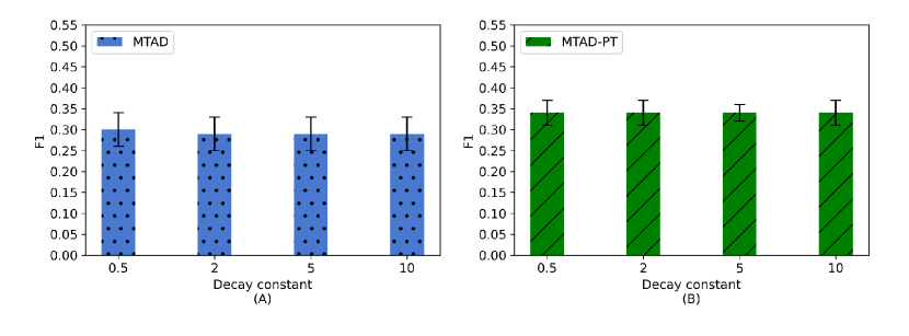
Figure 5: Comparing different decay constant values: (A) F1 score for MTAD (B) F1 score for MTAD-PT.

References

- Audibert et al. (2020) Julien Audibert, Pietro Michiardi, Frédéric Guyard, Sébastien Marti, and Maria A Zuluaga. Usad: Unsupervised anomaly detection on multivariate time series. In Proceedings of the 26th ACM SIGKDD International Conference on Knowledge Discovery & Data Mining, pages 3395–3404, 2020.
- Burghardt et al. (2021) Keith Burghardt, Nazgol Tavabi, Emilio Ferrara, Shrikanth Narayanan, and Kristina Lerman. Having a bad day? detecting the impact of atypical events using wearable sensors. In International Conference on Social Computing, Behavioral-Cultural Modeling and Prediction and Behavior Representation in Modeling and Simulation, pages 257–267. Springer, 2021.
- Castanho et al. (2021) Teresa Costa Castanho, Nadine Correia Santos, C Meleiro-Neves, S Neto, GR Moura, MA Santos, AR Cruz, Olga Cunha, A Castro Rodrigues, Ana João Rodrigues, et al. Association of positive and negative life events with cognitive performance and psychological status in late life: A cross-sectional study in northern portugal. Aging Brain, 1:100020, 2021.
- Chen et al. (2019) Guangyuan Chen, Guoliang Lu, Wei Shang, and Zhaohong Xie. Automated change-point detection of eeg signals based on structural time-series analysis. IEEE Access, 7:180168–180180, 2019.
- Cho et al. (2014) Kyunghyun Cho, Bart Van Merriënboer, Dzmitry Bahdanau, and Yoshua Bengio. On the properties of neural machine translation: Encoder-decoder approaches. arXiv preprint arXiv:1409.1259, 2014.
- Falkingham et al. (2020) Jane Falkingham, Maria Evandrou, Min Qin, and Athina Vlachantoni. Accumulated lifecourse adversities and depressive symptoms in later life among older men and women in england: a longitudinal study. Ageing & Society, 40(10):2079–2105, 2020.
- Faust et al. (2021) Louis Faust, Keith Feldman, Suwen Lin, Stephen Mattingly, Sidney D’Mello, and Nitesh V Chawla. Examining response to negative life events through fitness tracker data. Frontiers in digital health, 3:37, 2021.
- Fotoohinasab et al. (2020) Atiyeh Fotoohinasab, Toby Hocking, and Fatemeh Afghah. A graph-constrained changepoint detection approach for ecg segmentation. In 2020 42nd Annual International Conference of the IEEE Engineering in Medicine & Biology Society (EMBC), pages 332–336. IEEE, 2020.
- Goodyer (2001) Ian M Goodyer. Life events: Their nature and effects. The depressed child and adolescent, 2:204–232, 2001.
- Gupta et al. (2017) Arpana Gupta, Emeran A Mayer, and et al. Acosta, Jonathan R. Early adverse life events are associated with altered brain network architecture in a sex-dependent manner. Neurobiology of stress, 7:16–26, 2017.
- Hilbe (2009) Joseph M Hilbe. Logistic regression models. Chapman and hall/CRC, 2009.
- Hill (2002) McGraw Hill. Mcgraw hill concise medical dictionary of modern medicine, 2002.
- Hobson et al. (2001) Charles J Hobson, Linda Delunas, and Dawn Kesic. Compelling evidence of the need for corporate work/life balance initiatives: results from a national survey of stressful life-events. Journal of employment counseling, 38(1):38–44, 2001.
- Hochreiter and Schmidhuber (1997) Sepp Hochreiter and Jürgen Schmidhuber. Long short-term memory. Neural computation, 9(8):1735–1780, 1997.
- Karasek et al. (1981) Robert Karasek, Dean Baker, Frank Marxer, Anders Ahlbom, and Tores Theorell. Job decision latitude, job demands, and cardiovascular disease: a prospective study of swedish men. American journal of public health, 71(7):694–705, 1981.
- Katana et al. (2019) Marko Katana, Christina Röcke, Seth M Spain, and Mathias Allemand. Emotion regulation, subjective well-being, and perceived stress in daily life of geriatric nurses. Frontiers in psychology, 10:1097, 2019.
- Liu et al. (2008) Fei Tony Liu, Kai Ming Ting, and Zhi-Hua Zhou. Isolation forest. In 2008 eighth ieee international conference on data mining, pages 413–422. IEEE, 2008.
- Ma and Perkins (2003) Junshui Ma and Simon Perkins. Time-series novelty detection using one-class support vector machines. In Proceedings of the International Joint Conference on Neural Networks, 2003., volume 3, pages 1741–1745. IEEE, 2003.
- Malhotra et al. (2016) Pankaj Malhotra, Anusha Ramakrishnan, Gaurangi Anand, Lovekesh Vig, Puneet Agarwal, and Gautam Shroff. Lstm-based encoder-decoder for multi-sensor anomaly detection. arXiv preprint arXiv:1607.00148, 2016.
- Mattingly et al. (2019) Stephen M Mattingly, Julie M Gregg, Pino Audia, Ayse Elvan Bayraktaroglu, Andrew T Campbell, Nitesh V Chawla, Vedant Das Swain, Munmun De Choudhury, Sidney K D’Mello, Anind K Dey, et al. The tesserae project: Large-scale, longitudinal, in situ, multimodal sensing of information workers. In Extended Abstracts of the 2019 CHI Conference on Human Factors in Computing Systems, pages 1–8, 2019.
- Mirjafari et al. (2019) Shayan Mirjafari, Kizito Masaba, Ted Grover, Weichen Wang, Pino Audia, Andrew T Campbell, Nitesh V Chawla, Vedant Das Swain, Munmun De Choudhury, Anind K Dey, et al. Differentiating higher and lower job performers in the workplace using mobile sensing. Proceedings of the ACM on Interactive, Mobile, Wearable and Ubiquitous Technologies, 3(2):1–24, 2019.
- Nepal et al. (2020) Subigya Nepal, Shayan Mirjafari, Gonzalo J Martinez, Pino Audia, Aaron Striegel, and Andrew T Campbell. Detecting job promotion in information workers using mobile sensing. Proceedings of the ACM on Interactive, Mobile, Wearable and Ubiquitous Technologies, 4(3):1–28, 2020.
- Pang et al. (2021) Guansong Pang, Chunhua Shen, Longbing Cao, and Anton Van Den Hengel. Deep learning for anomaly detection: A review. ACM Computing Surveys (CSUR), 54(2):1–38, 2021.
- Park et al. (2018) Daehyung Park, Yuuna Hoshi, and Charles C Kemp. A multimodal anomaly detector for robot-assisted feeding using an lstm-based variational autoencoder. IEEE Robotics and Automation Letters, 3(3):1544–1551, 2018.
- Rumelhart et al. (1985) David E Rumelhart, Geoffrey E Hinton, and Ronald J Williams. Learning internal representations by error propagation. Technical report, California Univ San Diego La Jolla Inst for Cognitive Science, 1985.
- Sadhu et al. (2019) Vidyasagar Sadhu, Teruhisa Misu, and Dario Pompili. Deep multi-task learning for anomalous driving detection using can bus scalar sensor data. In 2019 IEEE/RSJ International Conference on Intelligent Robots and Systems (IROS), pages 2038–2043, 2019. 10.1109/IROS40897.2019.8967753.
- Shvetsov et al. (2020) Nikolay Shvetsov, Nazar Buzun, and Dmitry V. Dylov. Unsupervised non-parametric change point detection in electrocardiography. In 32nd International Conference on Scientific and Statistical Database Management, SSDBM 2020, New York, NY, USA, 2020. Association for Computing Machinery. ISBN 9781450388146. 10.1145/3400903.3400917.
- Spector and Fox (2002) Paul E Spector and Suzy Fox. An emotion-centered model of voluntary work behavior: Some parallels between counterproductive work behavior and organizational citizenship behavior. Human resource management review, 12(2):269–292, 2002.
- Srivastava et al. (2015) Nitish Srivastava, Elman Mansimov, and Ruslan Salakhudinov. Unsupervised learning of video representations using lstms. In International conference on machine learning, pages 843–852. PMLR, 2015.
- Steptoe and Kivimäki (2012) Andrew Steptoe and Mika Kivimäki. Stress and cardiovascular disease. Nature Reviews Cardiology, 9(6):360–370, 2012.
- Steptoe and Kivimäki (2013) Andrew Steptoe and Mika Kivimäki. Stress and cardiovascular disease: an update on current knowledge. Annual review of public health, 34:337–354, 2013.
- Stival et al. (2022) Mattia Stival, Mauro Bernardi, and Petros Dellaportas. Doubly-online changepoint detection for monitoring health status during sports activities. arXiv preprint arXiv:2206.11578, 2022.
- Su et al. (2019) Ya Su, Youjian Zhao, Chenhao Niu, Rong Liu, Wei Sun, and Dan Pei. Robust anomaly detection for multivariate time series through stochastic recurrent neural network. In Proceedings of the 25th ACM SIGKDD International Conference on Knowledge Discovery & Data Mining, KDD ’19, page 2828–2837, New York, NY, USA, 2019. Association for Computing Machinery. ISBN 9781450362016. 10.1145/3292500.3330672.
- Ugwu (2017) Fabian O Ugwu. Contribution of perceived high workload to counterproductive work behaviors: Leisure crafting as a reduction strategy. Practicum Psychologia, 7(2):1–17, 2017.
- Wu et al. (2021) Junfeng Wu, Li Yao, Bin Liu, Zheyuan Ding, and Lei Zhang. Multi-task learning based encoder-decoder: A comprehensive detection and diagnosis system for multi-sensor data. Advances in Mechanical Engineering, 13(5):16878140211013138, 2021.
- Zhou and Paffenroth (2017) Chong Zhou and Randy C Paffenroth. Anomaly detection with robust deep autoencoders. In Proceedings of the 23rd ACM SIGKDD international conference on knowledge discovery and data mining, pages 665–674, 2017.
- Zong et al. (2018) Bo Zong, Qi Song, Martin Renqiang Min, Wei Cheng, Cristian Lumezanu, Daeki Cho, and Haifeng Chen. Deep autoencoding gaussian mixture model for unsupervised anomaly detection. In International conference on learning representations, 2018.