Probabilistic Uncertainty Quantification of Prediction Models with Application to Visual Localization

Abstract

The uncertainty quantification of prediction models (e.g., neural networks) is crucial for their adoption in many robotics applications. This is arguably as important as making accurate predictions, especially for safety-critical applications such as self-driving cars. This paper proposes our approach to uncertainty quantification in the context of visual localization for autonomous driving, where we predict locations from images. Our proposed framework estimates probabilistic uncertainty by creating a sensor error model that maps an internal output of the prediction model to the uncertainty. The sensor error model is created using multiple image databases of visual localization, each with ground-truth location. We demonstrate the accuracy of our uncertainty prediction framework using the Ithaca365 dataset, which includes variations in lighting, weather (sunny, snowy, night), and alignment errors between databases. We analyze both the predicted uncertainty and its incorporation into a Kalman-based localization filter. Our results show that prediction error variations increase with poor weather and lighting condition, leading to greater uncertainty and outliers, which can be predicted by our proposed uncertainty model. Additionally, our probabilistic error model enables the filter to remove ad hoc sensor gating, as the uncertainty automatically adjusts the model to the input data.

I Introduction

The evolution of modern prediction models (e.g., neural networks) has revolutionized the performance of applications ranging from medical diagnostics, business analysis to robotics. However, much of the research in this field has focused primarily on enhancing performance (e.g., average prediction accuracy) through better data collection and architectures. Despite these advancements, one significant weakness of many models is their inability to provide a sense of confidence in individual predictions. Predictive accuracies of these models can vary based on factors such as the amount and diversity of training data, the model architecture details, and the complexity of the test environment [1, 2].

In certain applications, such as medical imaging or self-driving, probabilistic uncertainty quantification of prediction outputs is crucial. Realizing uncertainty models for these networks will not only facilitate their integration into formal probabilistic perception and planning frameworks but also enable better reasoning over the outputs. For example, in medical diagnosis, doctors should intervene when the neural network lacks confidence in its prediction [3]. While some modern neural networks attempt to output probabilistic uncertainty, the reliability of the uncertainty prediction is still insufficient for safety-critical decision-making [4]. Most modern neural networks are deterministic or produce only non-probabilistic confidence, such as the softmax function.

Current uncertainty modeling methods can generally be divided into three categories: Bayesian neural networks, ensemble, and post-processing methods. Bayesian neural networks [5, 6] construct an inherent uncertainty estimation framework by formalizing a probability distribution over the model parameters [7]. However, they are difficult to train and often output poorly calibrated confidence scores [8]. Ensemble methods [9] typically train multiple neural networks with different training data or architectures, and the variance of the networks’ output can indicate the uncertainty level. However, these methods require larger networks and additional training and inference steps. Post-processing methods, such as neural network calibration, are general enough to be used with different networks. However, they require uncalibrated uncertainty as an input and cannot predict uncertainty directly. Examples include histogram binning [10] and isotonic regression [11]. Some post-processing methods, such as Platt scaling [12], can predict uncertainty directly but require additional layers to be trained. The output of these methods is typically a simple confidence score, which is calibrated to be an approximate probability of correctness.

This paper presents a general uncertainty prediction framework that does not require additional training of the network or changes in network architecture. The framework is probabilistically formulated to provide both probability/confidence and an uncertainty distribution across the outputs. To achieve this, we leverage the concept of sensor models in estimation frameworks (e.g., Kalman filter). For traditional sensors, manufacturers typically provide error model specifications that indicate the accuracy of the sensor under different conditions, e.g. the accuracy of LiDAR as a function of range or the covariance of pseudo-ranges for GPS in various weather conditions. We propose creating an error uncertainty model for the network predictions using the internal network outputs and analysis across datasets.

We demonstrate the effectiveness of our uncertainty prediction approach using the problem of visual localization [13]. We focus on this problem for two reasons: first, the neural network outputs a 2D position from an image, making it easy to analyze, and second, the network’s performance is known to degrade in poor weather and lighting conditions[14, 15]. We build upon a typical visual localization model [16] which predicts the pose of a query image by searching the most similar image from a database of images with known poses using keypoint matching [17]. Firstly, we analyze the performance of a baseline neural network to understand its performance over different databases (weather and lighting). We then create a statistical error model using the internal outputs of the network (number of keypoint matches between the query and retrieved images) as the cue to predict visual localization error uncertainty. Importantly, the matched keypoints of each model/database can be calibrated and binned based on both a probability and 2D error. During inference, given the number of keypoint matches from an image, the sensor error model can directly return an uncertainty estimate in the form of a 2D error covariance (analogous to a traditional sensor) and a formal confidence. We can also incorporate the error model output in a Kalman-based localization filter, which provides a range of formal evaluation tools such as filter integrity and sensor hypothesis testing. We evaluate our approach using Ithaca365 [18], a large-scale real-world self-driving dataset that includes multiple traversals along repeated routes, varying weather and lighting conditions, and high precision GPS.

Our main contributions are three-folded: First, we analyze a state-of-the-art neural network for visual localization across a comprehensive dataset that includes multiple routes, lighting, and weather conditions to understand how errors vary across these key conditions. Second, we propose an approach to predict well-calibrated uncertainty without modifying the base neural network or requiring additional training. Third, we validate our method in the visual localization problem on a large real-world dataset under various settings and demonstrate that it consistently produces well-calibrated uncertainty estimates and high integrity filters without ad hoc fixes.

II Related Works

II-A Uncertainty Modeling.

Modern prediction models are known for their high performance in various tasks, but they often lack the ability to tell the uncertainty in their predictions. While some models, such as classification neural networks, can produce a confidence score, it is not probabilistic and therefore may not be entirely reliable. Ensembles [9, 19, 20] offer a solution by training multiple networks and combining their predictions to calculate variance and represent uncertainty. However, ensembles require more costly training steps for training multiple networks, as well as more inference time. Bayesian neural networks (BNNs) [5, 6] offer another potential solution by treating neural network weights as random variables instead of deterministic values, with predictions in the form of an expectation over the posterior distribution of the model weights. Two prominent methods in BNN are Bayes by Backprop [21] and Monte Carlo (MC) Dropout [22]. Bayes by Backprop regularises the weights by minimising the expected lower bound on the marginal likelihood. MC Dropout interprets dropout approximately as integrates over the models’ weights. However, BNN requires specifying a meaningful prior for the parameters which can be challenging. Additionally, the uncertainty is often poorly calibrated, necessitating post-processing methods [8, 23, 24] to map poorly calibrated uncertainty to well-calibrated uncertainty. For instance, temperature scaling is a widely used post-processing methods due to its simplicity and effectiveness [23] . [8] extends the technique from just classification tasks to regression tasks. However, such post-processing methods either require inputs of uncalibrated uncertainty or re-training some layers. In contrast, our method differs from these methods in that we do not alter the prediction model’s structure, hence preserving its performance. Furthermore, our method can output accurate uncertainty with no additional training and can be applied to any prediction models.

II-B Visual Localization

Visual localization aims to predict the pose of a query image using environmental information such as images and point clouds. Two main branches of visual localization are image-based localization and 3D-structure-based localization. Image-based localization [25, 26, 27] can be understood as an image retrieval problem, i.e. retrieving the most similar image from an image database/library with known poses and taking the pose of the retrieved image as the predicted pose. Several approaches [28, 29] have been proposed to extract image features for this purpose In contrast, 3D-structure-based localization [30, 31, 32, 33, 34, 35, 16] predicts the location by finding the pose that best matches the detected 2D keypoints in the query image with the 3D keypoints in a pre-constructed 3D model. However, to the best of our knowledge, few works have considered the uncertainty associated with the predicted location. While some works [17, 36] output confidence scores on detected keypoints and their matching, they do not provide any information about the uncertainty of the predicted location.

III Method

In this section, we discuss our method for uncertainty quantification of prediction models, using visual localization as the application task. We start by defining a baseline visual localization framework, then present our approach to modeling the errors and calibrating the uncertainties of the predictive network, and finally, we define a full visual localization pipeline, with a filter and sensor gating, to be used in the validation steps.

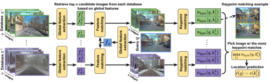
Figure 1: Pipeline for location prediction form image-retrieval using multiple traversals.

III-A Location Prediction from Image Retrieval

Let $X=\{k_{i}\}_{i=1}^{N}$ be a set of database images with known GPS locations $r(k_{i})$. Given a query image $q$, our goal is to estimate the location where the image was taken. As images taken from close-by poses should preserve some content similarity, we find the closest image $f_{\text{closest}}(q;X)$ from database $X$ and use its corresponding location as the predicted location $\hat{r}(q)=r(f_{\text{closest}}(q;X))$. We define the closest image as the image with the most number of keypoint matches $n_{\text{kpm}}$ to the query image. However, performing keypoint matching of the query image to all $N$ database images is computationally expensive. Therefore, more efficient global feature matching (NetVLAD [29]) is performed first, followed by neural keypoint matching (SuperPoint[36] + SuperGlue [17]) on the top $n\!<<\!N$ candidate images. This pipeline is shown in Figure 1 (top, green).

A standard location prediction from image retrieval pipeline typically uses a database from just one traversal (passing the route once). We propose to use multiple databases from multiple traversals, motivated by several key observations. First, a query image has a non-zero distance to even its closest image from a database (see Figure 2). Using multiple traversals increases the database image options and thus lowers the average error. Second, as the query image for localization can originate from different weather and lighting conditions, it is important to diversify the database images to reduce potential errors (those from the traversal and from keypoint mismatches). Finally and most importantly, data from multiple traversals can be used to provide a localization uncertainty prediction, as will be shown in III-B.

One naive approach is to simply treat the additional data from multiple traversals $X^{1},X^{2},\dots,X^{L}$ as one combined (large) database, and apply the same pipeline. However, this is not effective, as the candidate images retrieved by global feature matching often are biased to come from a single database whose color or even foreground object appearance is most similar to the query image. This motivates our new approach that encourages retrieval of candidate images from each traversal as shown in Figure 1.

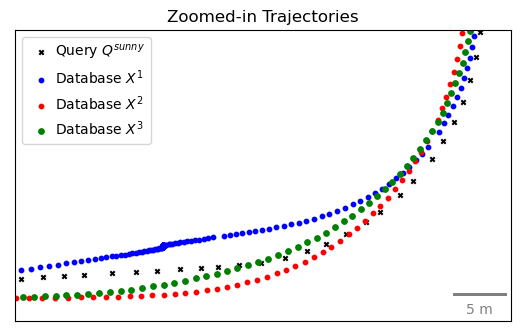
Figure 2: GPS locations of several traversals (zoomed in for illustration; full trajectory is not shown). Using multiple traversals increases the chances that a database image is closer to the query image location (i.e., smaller theoretical error).

III-B Uncertainty Prediction and Quantification

III-B1 Problem Definition

We formally define the uncertainty quantification problem as predicting the error bound $\sigma_{c}(q)\in\mathbb{R}^{+}$ of image $q$ and confidence level $c\in[0,1]$ such that the error between the predicted location $\hat{r}=r(f(q;X))$ and the ground-truth $r_{\text{gt}}$ is below $\sigma_{c}$ by $c$ probability:

$$p\left(\lVert\hat{r}-r_{\text{gt}}\rVert<\sigma_{c}(q)\right)=c$$ (1)

III-B2 Sensor Error Model

We propose to create a sensor error model to determine the confidence of the prediction (e.g. neural network output). A sensor error model maps key attributes of prediction to error bound $\sigma_{c}$ and confidence $c$ estimates; for example, the error of stereo depth sensor is quadratic to range [37]. We first analyze the performance of visual localization prediction as a function of the number of keypoint matches $n_{\text{kpm}}$ by performing cross-validation using different databases. As an example, Figure 3 shows scatter plots of the location error between images from two databases (sunny and night) and their closest images from another database (sunny) as a function of the number of keypoint matches.

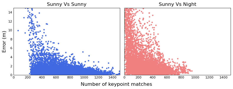
Figure 3: Relationship between number of keypoint matches and location error for two different database traversals.

From this analysis, we learn two things. First, the number of keypoint matches $n_{\text{kpm}}$ can serve as a good indicator for uncertainty quantification. Second, the relationship between number of keypoint matches and error can be different for different databases (traversals); the scatter plots have different distributions. Thus, we propose to build the sensor error model as a function of number of keypoint matches, and build one model for each different traversal. We can utilize multiple traversals to learn this mapping as follows.

III-B3 Creating Sensor Error Model

Key to our approach is creating a sensor error model for each database/traversal. For database $l$, we apply the image retrieval pipeline using traversal $X^{l}$ as the query and another traversal $X^{m\neq l}$ as the database. For every image $k_{i}^{l}\in X^{l}$, we find the closest image $f(k_{i}^{l};X^{m})$ from database $m$ and compute the location error $\lVert r(f(k_{i}^{l};X^{m}))-r(k_{i}^{l})\rVert$. Thus, for each image, we can compute the number of keypoint matches (to its closest image) and location error. This process is repeated using all $L-1$ different traversals (other than $X_{l}$). We divide the data (number of keypoints vs error) into bins according to the number of keypoint matches (e.g., bin 1 contains data points with keypoint matches ranging from 0-200, bin 2 from 200-400, and so on). For each bin, we empirically determine the error bound $\sigma_{c}$ for confidence $c$ such that $c$ fraction of data in that bin has smaller error than $\sigma_{c}$. We repeat for each traversal/database, as shown in Figure 4(top).

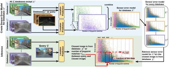
Figure 4: Pipeline for uncertainty prediction. Top: creating sensor error model. Bottom: using sensor error model in inference.

III-B4 Model Prediction with Uncertainty and Confidence

The inference process is shown in Figure 4(bottom). Given a query image of unknown location, we retrieve the closest image (as detailed in III-A); the location of the closest image becomes the predicted location. To find the confidence of the prediction, we use the database of the closest image (say $l$, or $X^{l}$). The corresponding ($l$) sensor error model is then used; the bin associated with the number of keypoint matches (between query and closest image) gives the corresponding error bound $\sigma_{c}$ at confidence level $c$.

Finally, we form a quantified uncertainty (in the form of a 2D estimation error covariance in this case). Specifically, we compute the measurement covariance $R\in\mathbb{R}^{2\times 2}$ from the cross-validation data, per database, per number of keypoint matches range (bin). The covariance matrices are formed and expressed in the ego car (sensor) coordinates. This covariance matrix will be used as the measurement covariance in subsection III-C.

III-C Full Visual Localization Pipeline

We build a full visual localization pipeline using the location prediction (III-A) as the uncertain measurement, the uncertainty prediction (III-B) as the error covariance, within a formal estimation framework using the Sigma Point (Unscented) filter (SPF) [38, 39]. Our goal is to estimate the $p(s_{t}|m_{1:t})$ of the state vector $s_{t}$ at time $t$ given observed measurements $m_{1:t}$. We define the state vector as follows:

$$s=\begin{bmatrix}x&y&\theta&v&\dot{\theta}\end{bmatrix}^{T}$$ (2)

where $x,y,\theta$ are the inertial, planar position and heading angle, and $v,\dot{\theta}$ are the linear and angular velocity of the car. In the prediction step of the SPF, we assume constant linear and angular velocity ($v$ and $\dot{\theta}$) with a small process noise. In the measurement update, given an image input, we process the image through the location and uncertainty prediction pipeline (III-A and III-B) to give the ($x,y$) location measurement and error covariance; the covariance is transformed to the inertial coordinates for the filter.

Most modern estimation frameworks also typically employ sensor measurement gating to decide whether to accept a measurement (i.e., use it in the filter update) or reject the measurement (i.e., it is an outlier, outside the nominal error mode). Given a measurement vector $m$, we compute the Mahalanobis distance $d_{M}$ defined as follows:

$$d_{\textrm{M}}^{2}=(m-\hat{m})^{T}(H\hat{C}H^{T}+R)^{-1}(m-\hat{m})$$ (3)

where $R$ is the measurement covariance transformed to the world coordinate, $\hat{C}$ is the estimated state covariance from the SPF, $H$ is the measurement matrix that maps the state vector to the measurement, and $\hat{m}=Hs$ is the expected measurement. The measurement is rejected if it lies outside of the validation gate,

$$\text{if }d_{\textrm{M}}^{2}>\chi^{2}_{k,\alpha}\rightarrow\text{reject},$$ (4)

where $\chi^{2}_{k,\alpha}$ is a threshold from the inverse chi-squared cumulative distribution at a level $\alpha$ with $k$ degrees of freedom. The level $\alpha$ controls the validation gate, i.e. it rejects $(1\!-\!\alpha)\times 100\%$ of the measurements at the tail; typical values are $0.99$, $0.975$, and $0.95$.

IV Experiments

IV-A Dataset

We use the Ithaca365 dataset [18], containing data collected over multiple traversals along a 15km route under various conditions: snowy, rainy, sunny, and nighttime. We utilize two types of sensor data, images, and GPS locations for our experiments. For our database, we randomly select nine traversals, with three traversals each from the sunny ($X^{1}$, $X^{2}$, $X^{3}$), nighttime ($X^{4}$, $X^{5}$, $X^{6}$), and snowy ($X^{7}$, $X^{8}$, $X^{9}$). We use three additional traversals ($Q^{\text{sunny}}$, $Q^{\text{snow}}$ and $Q^{\text{night}}$), one from each condition, as queries for testing and evaluation. To avoid double counting and ensure a uniform spatial distribution across the scenes in evaluation, we sample query images at an interval of $\approx$1m, except for highways where the spacing is larger. This results in an average of $\approx$10,000 images for each query traversal, $Q^{(\cdot)}$.

IV-B Evaluation

IV-B1 Sensor Error Model

First, we evaluate the correctness of our uncertainty prediction on location prediction using image retrieval. Following [8, 23], we use reliability diagram to compare the expected confidence level with the observed confidence level. For a given expected confidence level $c$, the observed confidence is obtained by computing the empirical frequency $\hat{p}_{c}$ that the location error $\lVert\hat{x}(q)-x_{\text{gt}}(q)\rVert$ is below the predicted uncertainty $\sigma_{c}(q)$:

$$\hat{p}_{c}=\frac{\left|\{q\in Q\ \text{ s.t. }\lVert\hat{x}(q)-x_{\text{gt}}(q)\rVert\leq\sigma_{c}(q)\}\right|}{|Q|}.$$ (5)

If the uncertainty quantification is accurate, the diagram should plot the identity function (a straight line with a gradient of one). The reliability diagram in Figure 5 shows that our method produces accurate probabilistic confidence, as evidenced by the small gaps between observed and expected confidence at all levels and across all three conditions.

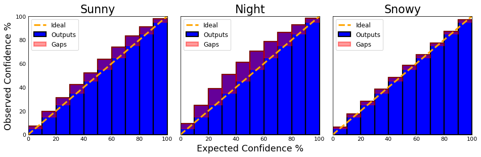
Figure 5: Reliability diagrams for $Q^{\text{sunny}}$, $Q^{\text{night}}$, and $Q^{\text{snowy}}$.

IV-B2 Visual Localization: Filter + Prediction/Error Model

Next, we evaluate the full visual localization pipeline, which uses the previous location predictions as measurements in the SPF (subsection III-C). We evaluate both the localization error and the uncertainty of the estimates. The localization error $d_{\text{err}}$ is the average distance error between estimated and ground-truth locations, whereas covariance credibility measures the frequency that the 2D localization error lies within an $n$-sigma covariance ellipse; we use 1-, 2- and 3-sigma, corresponding to $68\%$, $95\%$ and $99.7\%$ probability respectively in a 2D Gaussian distribution.

We present three sets of experiments in Table I. The first set of experiments (rows 1-9) uses the original image inputs. The second and the third sets simulate high sensor error/failure by corrupting several images along the red paths of Figure 7. Specifically, the second set (rows 10-15) applies average blurring, and the third set (rows 16-21) applies salt and pepper noise, as shown in Figure 7. Within each set, three sets of measurement gating are evaluated, with 0, 1.0% and 2.5% probability gate. We compare our method to a constant covariance baseline commonly used in Kalman filter, where the constant covariance value is obtained by tuning on the validation data, separately for each weather condition. Our method and the constant covariance baseline receive the same measurement vectors but use different measurement covariance. Additionally, in the first experiment set, we provide a comparison to the Monte Carlo (MC) Dropout method. Specifically, we apply a dropout layer after the final keypoint feature projection layer with a 0.3 dropout probability and repeat the dropout process multiple times until the SPF localization results stabilize. We report the converged results.

TABLE I: Evaluation result of Unscented Kalman Filter localization for sunny, night, and snowy conditions.

Row	Method	Gating $(1-\alpha)$	$d_{\text{err}}$(m) $\downarrow$	Cov-credibility(%)	$n_{r}(\%)$	$d_{\text{err}}$(m) $\downarrow$	Cov-credibility(%)	$n_{r}(\%)$	$d_{\text{err}}$(m) $\downarrow$	Cov-credibility(%)	$n_{r}(\%)$
Normal measurement — Average measurement error: 0.83m / 11.67m / 1.76m for MC dropout – 0.87m / 8.68m / 1.42m for baseline and ours.
1	MC d.o	0	0.792	32.8 / 67.4 / 84.7	0	7.442	27.6 / 56.2 / 71.0	0	1.501	20.4 / 50.4 / 69.8	0
2	Baseline	0	0.766	46.1 / 81.2 / 92.3	0	8.425	38.5 / 67.0 / 78.9	0	1.302	30.5 / 61.8 / 79.6	0
3	Ours	0	0.569	62.2 / 91.4 / 97.4	0	3.075	75.9 / 94.6 / 98.6	0	0.811	55.4 / 86.4 / 95.9	0
4	MC d.o	1.0%	0.612	33.1 / 68.2 / 85.6	1.0	165.282	23.4 / 46.0 / 57.7	33.0	1.442	21.2 / 51.6 / 71.6	4.8
5	Baseline	1.0%	0.610	46.6 / 82.1 / 93.3	1.0	54.382	33.9 / 57.2 / 67.0	30.3	333.538	17.5 / 38.3 / 51.7	37.7
6	Ours	1.0%	0.570	62.3 / 91.4 / 97.5	0.2	2.926	76.2 / 94.6 / 98.7	0.3	222.608	34.5 / 56.4 / 63.9	33.2
7	MC d.o	2.5%	0.613	33.1 / 68.2 / 85.9	1.5	7607.294	3.6 / 8.5 / 11.5	86.7	8144.861	3.7 / 9.0 / 12.3	82.5
8	Baseline	2.5%	790.307	32.8 / 54.5 / 61.6	35.2	54.205	34.1 / 57.9 / 69.1	31.3	8169.233	5.1 / 11.2 / 14.8	82.3
9	Ours	2.5%	82.828	47.7 / 67.9 / 72.5	26.2	2.942	76.3 / 94.6 / 98.7	0.4	8121.261	7.6 / 14.1 / 16.7	82.0
Study case where 5.0% / 4.7% / 4.6% of data are corrupted with average blurring — Average measurement error: 108.21m / 121.78m / 108.66m
10	Baseline	0	107.163	41.9 / 74.6 / 85.4	0	121.370	36.3 / 63.5 / 74.4	0	108.080	29.2 / 58.9 / 75.3	0
11	Ours	0	3.371	61.0 / 90.3 / 96.9	0	7.702	72.9 / 92.7 / 97.2	0	3.351	56.4 / 87.0 / 95.7	0
12	Baseline	1.0%	1726.025	3.6 / 7.1 / 8.3	91.1	8776.021	1.8 / 2.6 / 3.4	97.2	726.828	14.9 / 28.9 / 37.0	58.7
13	Ours	1.0%	3.529	61.3 / 90.6 / 97.0	1.3	66.813	65.8 / 82.3/ 86.7	12.4	264.000	35.8 / 57.4 / 64.2	33.3
14	Baseline	2.5%	1756.856	6.0 / 8.0 / 8.9	91.4	1510.11	6.0 / 11.4 / 15.6	84.1	8169.514	5.5 / 11.6 / 15.0	83.3
15	Ours	2.5%	110.299	51.3 / 73.2 / 78.2	20.6	70.659	65.9 / 82.0 / 86.5	13.2	820.152	16.0 / 29.0 / 34.8	62.1
Study case where 5.0% / 4.7% / 4.6% of data are corrupted with salt and pepper noise — Average measurement error: 66.09m / 103.63m / 85.26m
16	Baseline	0	65.365	42.0 / 74.9 / 85.6	0	102.887	36.8 / 63.9 / 75.0	0	84.738	29.1 / 58.7 / 75.1	0
17	Ours	0	1.971	61.9 / 91.1 / 97.4	0	7.083	73.1 / 92.2 / 97.1	0	2.468	57.0 / 87.4 / 96.1	0
18	Baseline	1.0%	0.985	45.8 / 80.4 / 92.1	5.5	3563.210	24.6 / 36.2 / 40.2	60.4	724.023	15.1 / 29.3 / 38.0	56.7
19	Ours	1.0%	1.719	62.3 / 91.3 / 97.5	0.6	437.251	28.7 / 40.6 / 48.0	39.5	1329.145	13.3 / 17.7 / 18.8	76.7
20	Baseline	2.5%	420.962	35.2 / 58.2 / 66.7	33.7	1308.586	2.2 / 3.2 / 7.9	96.1	1554.474	2.2 / 3.8 / 6.4	94.5
21	Ours	2.5%	81.392	48.3 / 68.4 / 74.0	25.4	408.598	27.6 / 38.7 / 46.6	42.8	1110.267	7.4 / 13.4 / 17.6	79.9

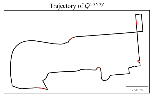
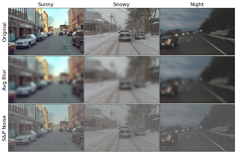
Figure 6: Data collection path (black), with corrupted images (red).

Figure 7: Examples of corrupted images. Top: original images. Mid: blurred images (average blur with kernel size 80, Bottom: images corrupted with salt and pepper noise (noise amount is 0.5)).

Analysis of Table I yields several observations. Firstly, our method outperforms the MC Dropout and constant covariance baselines in terms of localization accuracy ($d_{\text{err}}$) in nearly all cases, suggesting that a good uncertainty model can improve localization accuracy, even with similar measurement quality. Our method also produces more accurate uncertainty estimates (indicated by covariance-credibility) than the two baselines in nearly all cases. This is crucial for making informed decisions in the future. Second, we observe that formal sensor gating through hypothesis testing with prediction networks is too sensitive and does not work well. However, our adaptive covariance method removes the need for sensor gating and standard outlier rejection in filters. In the typical estimation framework, sensor gating is used to reject bad measurements that could adversely affect the performance. While outlier rejection may improve performance, it is highly susceptible to threshold parameter selection ($\chi^{2}_{k,\alpha}$). We observe that there is hardly a single appropriate threshold value that works for different query and measurement conditions. The analysis of the chi-square test using errors and covariances indicates that the errors produced by the DL algorithm do not conform to a Gaussian error model, which is essential to the chi-square test. This finding suggests potential future work in developing non-Gaussian uncertainty models and associated gating techniques that can better match the DL errors.

Fortunately, a key novelty of our approach is that it does not require a formal outlier rejection method. Our approach automatically adjusts the error covariance based on the number of keypoints, which addresses the uncertainty of the measurement, even if it is an outlier. We argue that this is a key contribution for two reasons. First, it is clear that outlier prediction is highly sensitive. Second, even noisy, uncertain measurements can still contain useful information. Our uncertainty modeling approach allows the filter to incorporate all prediction outputs, resulting in better performance and more robust applications.

IV-B3 Latency and Data Size

On a 1080Ti GPU, extracting global features of an image using NetVLAD takes about 8ms, while performing keypoint matching for a single pair of images using SuperPoint and SuperGlue takes approximately 112ms. Although keypoint matching is done between a query image and ten candidate images, the GPU can simultaneously process them in a batch without affecting the speed. The database comprises 127,225 images with a total size of 417.7 GB. Instead of storing the original images, we only need to store the extracted global features (2.24GB) and the keypoint features (161.9GB).

V Conclusion

We present a general and formal probabilistic approach for modeling prediction (e.g., neural network) uncertainties, which we validate in the context of visual localization problem. Our approach involves creating a sensor error model that maps the output of the internal prediction model (number of keypoint matches) to probabilistic uncertainty for each database. During inference, we use the sensor error model to map the number of keypoint matches to confidence probability and 2D covariance. We evaluate our approach using a large-scale real-world self-driving dataset with varying weather, lighting, and sensor corruption conditions, demonstrating accurate uncertainty predictions across all conditions. Notably, our approach of creating a different error covariance tailored to each measurement eliminates the need for sensor gating, which is overly sensitive due to their non-Gaussian nature. Our approach results in more robust and better-performing perception pipelines.

References

- [1] Yan Wang, Xiangyu Chen, Yurong You, Li Erran, Bharath Hariharan, Mark Campbell, Kilian Q. Weinberger, and Wei-Lun Chao. Train in germany, test in the usa: Making 3d object detectors generalize, 2020.
- [2] Judy Hoffman, Eric Tzeng, Taesung Park, Jun-Yan Zhu, Phillip Isola, Kate Saenko, Alexei A. Efros, and Trevor Darrell. Cycada: Cycle-consistent adversarial domain adaptation, 2017.
- [3] Xiaoqian Jiang, Melanie Osl, Jihoon Kim, and Lucila Ohno-Machado. Calibrating predictive model estimates to support personalized medicine. Journal of the American Medical Informatics Association : JAMIA, 19:263–74, 03 2012.
- [4] Deng-Bao Wang, Lei Feng, and Min-Ling Zhang. Rethinking calibration of deep neural networks: Do not be afraid of overconfidence. In M. Ranzato, A. Beygelzimer, Y. Dauphin, P.S. Liang, and J. Wortman Vaughan, editors, Advances in Neural Information Processing Systems, volume 34, pages 11809–11820. Curran Associates, Inc., 2021.
- [5] David J. C. MacKay. A Practical Bayesian Framework for Backpropagation Networks. Neural Computation, 4(3):448–472, 05 1992.
- [6] Radford M. Neal. Bayesian Learning for Neural Networks. Springer-Verlag, Berlin, Heidelberg, 1996.
- [7] Jakob Gawlikowski, Cedrique Rovile Njieutcheu Tassi, Mohsin Ali, Jongseo Lee, Matthias Humt, Jianxiang Feng, Anna M. Kruspe, Rudolph Triebel, Peter Jung, Ribana Roscher, M. Shahzad, Wen Yang, Richard Bamler, and Xiaoxiang Zhu. A survey of uncertainty in deep neural networks. ArXiv, abs/2107.03342, 2021.
- [8] Volodymyr Kuleshov, Nathan Fenner, and Stefano Ermon. Accurate uncertainties for deep learning using calibrated regression. In Jennifer Dy and Andreas Krause, editors, Proceedings of the 35th International Conference on Machine Learning, volume 80 of Proceedings of Machine Learning Research, pages 2796–2804. PMLR, 10–15 Jul 2018.
- [9] Balaji Lakshminarayanan, Alexander Pritzel, and Charles Blundell. Simple and scalable predictive uncertainty estimation using deep ensembles. In Proceedings of the 31st International Conference on Neural Information Processing Systems, NIPS’17, page 6405–6416, Red Hook, NY, USA, 2017. Curran Associates Inc.
- [10] Bianca Zadrozny and Charles Peter Elkan. Obtaining calibrated probability estimates from decision trees and naive bayesian classifiers. In ICML, 2001.
- [11] Bianca Zadrozny and Charles Elkan. Transforming classifier scores into accurate multiclass probability estimates. Proceedings of the ACM SIGKDD International Conference on Knowledge Discovery and Data Mining, 08 2002.
- [12] John C. Platt. Probabilistic outputs for support vector machines and comparisons to regularized likelihood methods. In ADVANCES IN LARGE MARGIN CLASSIFIERS, pages 61–74. MIT Press, 1999.
- [13] Tayyab Naseer, Wolfram Burgard, and Cyrill Stachniss. Robust visual localization across seasons. IEEE Transactions on Robotics, 34(2):289–302, 2018.
- [14] Martin Humenberger, Yohann Cabon, Nicolas Guerin, Julien Morat, Vincent Leroy, Jérôme Revaud, Philippe Rerole, Noé Pion, Cesar de Souza, and Gabriela Csurka. Robust image retrieval-based visual localization using kapture, 2020.
- [15] Tianxin Shi, Hainan Cui, Zhuo Song, and Shuhan Shen. Dense semantic 3d map based long-term visual localization with hybrid features, 2020.
- [16] Paul-Edouard Sarlin, Cesar Cadena, Roland Siegwart, and Marcin Dymczyk. From coarse to fine: Robust hierarchical localization at large scale. In 2019 IEEE/CVF Conference on Computer Vision and Pattern Recognition (CVPR), pages 12708–12717, 2019.
- [17] Paul-Edouard Sarlin, Daniel DeTone, Tomasz Malisiewicz, and Andrew Rabinovich. Superglue: Learning feature matching with graph neural networks, 2019.
- [18] Carlos A. Diaz-Ruiz, Youya Xia, Yurong You, Jose Nino, Junan Chen, Josephine Monica, Xiangyu Chen, Katie Luo, Yan Wang, Marc Emond, Wei-Lun Chao, Bharath Hariharan, Kilian Q. Weinberger, and Mark Campbell. Ithaca365: Dataset and driving perception under repeated and challenging weather conditions. In Proceedings of the IEEE/CVF Conference on Computer Vision and Pattern Recognition (CVPR), pages 21383–21392, June 2022.
- [19] Matias Valdenegro-Toro. Deep sub-ensembles for fast uncertainty estimation in image classification. ArXiv, abs/1910.08168, 2019.
- [20] Yeming Wen, Dustin Tran, and Jimmy Ba. Batchensemble: An alternative approach to efficient ensemble and lifelong learning. ArXiv, abs/2002.06715, 2020.
- [21] Charles Blundell, Julien Cornebise, Koray Kavukcuoglu, and Daan Wierstra. Weight uncertainty in neural networks, 2015.
- [22] Yarin Gal and Zoubin Ghahramani. Dropout as a bayesian approximation: Representing model uncertainty in deep learning, 2016.
- [23] Chuan Guo, Geoff Pleiss, Yu Sun, and Kilian Q. Weinberger. On calibration of modern neural networks, 2017.
- [24] Matthias Minderer, Josip Djolonga, Rob Romijnders, Frances Hubis, Xiaohua Zhai, Neil Houlsby, Dustin Tran, and Mario Lucic. Revisiting the calibration of modern neural networks, 2021.
- [25] Relja Arandjelović and Andrew Zisserman. Three things everyone should know to improve object retrieval. In 2012 IEEE Conference on Computer Vision and Pattern Recognition, pages 2911–2918, 2012.
- [26] Hyo Jin Kim, Enrique Dunn, and Jan-Michael Frahm. Predicting good features for image geo-localization using per-bundle vlad. In 2015 IEEE International Conference on Computer Vision (ICCV), pages 1170–1178, 2015.
- [27] Filip Radenović, Giorgos Tolias, and Ondřej Chum. Cnn image retrieval learns from bow: Unsupervised fine-tuning with hard examples. In ECCV, 2016.
- [28] Akihiko Torii, Relja Arandjelović, Josef Sivic, Masatoshi Okutomi, and Tomas Pajdla. 24/7 place recognition by view synthesis. In 2015 IEEE Conference on Computer Vision and Pattern Recognition (CVPR), pages 1808–1817, 2015.
- [29] Relja Arandjelovic, Petr Gronat, Akihiko Torii, Tomas Pajdla, and Josef Sivic. Netvlad: Cnn architecture for weakly supervised place recognition. In 2016 IEEE Conference on Computer Vision and Pattern Recognition (CVPR), pages 5297–5307, 2016.
- [30] Arnold Irschara, Christopher Zach, Jan-Michael Frahm, and Horst Bischof. From structure-from-motion point clouds to fast location recognition. pages 2599–2606, 06 2009.
- [31] J. L. Schonberger, M. Pollefeys, A. Geiger, and T. Sattler. Semantic visual localization. In 2018 IEEE/CVF Conference on Computer Vision and Pattern Recognition (CVPR), pages 6896–6906, Los Alamitos, CA, USA, jun 2018. IEEE Computer Society.
- [32] Marcel Geppert, Peidong Liu, Zhaopeng Cui, Marc Pollefeys, and Torsten Sattler. Efficient 2d-3d matching for multi-camera visual localization. pages 5972–5978, 05 2019.
- [33] Uzair Nadeem, Mohammad Jalwana, Mohammed Bennamoun, Roberto Togneri, and Ferdous Sohel. Direct Image to Point Cloud Descriptors Matching for 6-DOF Camera Localization in Dense 3D Point Clouds, pages 222–234. 12 2019.
- [34] Hugo Germain, Guillaume Bourmaud, and Vincent Lepetit. Sparse-to-dense hypercolumn matching for long-term visual localization. pages 513–523, 09 2019.
- [35] Torsten Sattler, Michal Havlena, Filip Radenović, Konrad Schindler, and Marc Pollefeys. Hyperpoints and fine vocabularies for large-scale location recognition. 12 2015.
- [36] Daniel DeTone, Tomasz Malisiewicz, and Andrew Rabinovich. Superpoint: Self-supervised interest point detection and description. In 2018 IEEE/CVF Conference on Computer Vision and Pattern Recognition Workshops (CVPRW), pages 337–33712, 2018.
- [37] David Gallup, Jan-Michael Frahm, Philippos Mordohai, and Marc Pollefeys. Variable baseline/resolution stereo. In 2008 IEEE conference on computer vision and pattern recognition, pages 1–8. IEEE, 2008.
- [38] Eric A Wan and Rudolph Van Der Merwe. The unscented kalman filter for nonlinear estimation. In Proceedings of the IEEE 2000 Adaptive Systems for Signal Processing, Communications, and Control Symposium (Cat. No. 00EX373), pages 153–158. Ieee, 2000.
- [39] Shelby Brunke and Mark E. Campbell. Square Root Sigma Point Filtering for Real-Time, Nonlinear Estimation. AIAA J. Guid. Control. Dyn., 27(2):314–317, mar 2004.