A Study of Bayesian Neural Network Surrogates
for Bayesian Optimization

Abstract

Bayesian optimization is a highly efficient approach to optimizing objective functions which are expensive to query. These objectives are typically represented by Gaussian process (GP) surrogate models which are easy to optimize and support exact inference. While standard GP surrogates have been well-established in Bayesian optimization, Bayesian neural networks (BNNs) have recently become practical function approximators, with many benefits over standard GPs such as the ability to naturally handle non-stationarity and learn representations for high-dimensional data. In this paper, we study BNNs as alternatives to standard GP surrogates for optimization. We consider a variety of approximate inference procedures for finite-width BNNs, including high-quality Hamiltonian Monte Carlo, low-cost stochastic MCMC, and heuristics such as deep ensembles. We also consider infinite-width BNNs and partially stochastic models such as deep kernel learning. We evaluate this collection of surrogate models on diverse problems with varying dimensionality, number of objectives, non-stationarity, and discrete and continuous inputs. We find: (i) the ranking of methods is highly problem dependent, suggesting the need for tailored inductive biases; (ii) HMC is the most successful approximate inference procedure for fully stochastic BNNs; (iii) full stochasticity may be unnecessary as deep kernel learning is relatively competitive; (iv) infinite-width BNNs are particularly promising, especially in high dimensions.

1 Introduction

Bayesian optimization [31] is a distinctly compelling success story of Bayesian inference. In Bayesian optimization, we place a prior over the objective we wish to optimize, and use a surrogate model to infer a posterior predictive distribution over the values of the objective at all feasible points in space. We then combine this predictive distribution with an acquisition function that trades-off exploration (moving to regions of high uncertainty) and exploitation (moving to regions with a high expected value, for maximization). The resulting approach converges quickly to a global optimum, with strong performance in many expensive black-box settings ranging from experimental design, to learning parameters for simulators, to hyperparameter tuning [7, 10].

While many acquisition functions have been proposed for Bayesian optimization [e.g. 8, 44], Gaussian processes (gps) with standard Matérn or RBF kernels are almost exclusively used by default as a surrogate model for the objective, without checking whether other alternatives would be more appropriate, despite the fundamental role that the surrogate model plays in Bayesian optimization.

Thus, despite promising advances in Bayesian optimization research, there is an elephant in the room: should we be considering other surrogate models? It has become particularly timely to evaluate Bayesian neural network (bnn) surrogates as alternatives to Gaussian processes with standard kernels: In recent years, there has been extraordinary progress in making bnns practical [e.g. 4, 17, 34, 42, 47]. Moreover, bnns can flexibly represent the non-stationary behavior typical of optimization objectives, discover similarity measures as part of representation learning which is useful for higher dimensional inputs, and naturally handle multi-output objectives. In parallel, new Monte-Carlo acquisition functions [1] have been developed which only require posterior samples, significantly lowering the barrier to using non-gp surrogates that do not provide closed-form predictive distributions.

In this paper, we exhaustively evaluate Bayesian neural networks as surrogate models for Bayesian optimization. We consider conventional fully stochastic multilayer bnns with a variety of approximate inference procedures, ranging from high-quality full-batch Hamiltonian Monte Carlo [15, 27, 28], to stochastic gradient Markov Chain Monte Carlo [3], to heuristics such as deep ensembles [21]. We also consider infinite-width bnns [22, 29], corresponding to gps with fixed non-stationary kernels derived from a neural network architecture, as well as partially Bayesian last-layer deep kernel learning methods [48]. This particularly wide range of neural network-based surrogates allows us to evaluate the role of representation learning, non-stationarity, and stochasticity in modeling Bayesian optimization objectives. Moreover, given that so much is unknown about the role of the surrogate model, we believe it is particularly valuable not to have a “horse in the race”, such as a special bnn model particularly designed for Bayesian optimization, in order to conduct an unbiased scientific study where any outcome is highly informative.

We also extensively study a variety of synthetic and real-world objectives—with a wide range of input space dimensionalities, single- and multi-dimensional output spaces, and both discrete and continuous inputs, and non-stationarities.

Our study provides several key findings: (1) while stochasticity is often prized in Bayesian optimization [10, 35], fully stochastic bnns do not consistently dominate deep kernel learning, which is not stochastic about network parameters, due to the small data sizes in Bayesian optimization; (2) of the fully stochastic bnns, hmc generally works the best for Bayesian optimization, and deep ensembles work surprisingly poorly, given their success in other settings; (3) on standard benchmarks, standard gps are relatively competitive, due to their strong priors and simple exact inference procedures; (4) there is no single method that dominates across most problems, demonstrating that there is significant variability across Bayesian optimization objectives, where tailoring the surrogate to the objective has particular value; (5) infinite-width bnns are surprisingly effective at high-dimensional optimization, even relative to dkl and stochastic multilayer bnns. These results suggest that the non-Euclidean similarity metrics constructed from neural networks are valuable for high-dimensional Bayesian optimization, but representation learning (provided by dkl and finite-width bnns) is not as valuable as a strong prior derived from a neural network architecture (provided by the infinite-width bnn).

This study also serves as an evaluation framework for considering alternative surrogate models for Bayesian optimization. Our code is available at https://github.com/yucenli/bnn-bo.

2 Related Work

There is a large body of literature on improving the performance of Bayesian optimization. However, an overwhelming majority of this research only considers Gaussian process surrogate models, focusing on developing new acquisition functions [e.g. 8, 44], additive covariance functions [9, 16], the inclusion of gradient information [49], multi-objectives [41], trust region methods that use input partitioning for higher dimensional and non-stationary data [6], and covariance functions for discrete inputs and strings [26]. For a comprehensive review, see Garnett [10].

There has been some prior work focusing on other types of surrogate models for Bayesian optimization, such as random forests [13] and tree-structured Parzen estimators [2]. Moreover, Snoek et al. [36] apply a Bayesian linear regression model to the last layer of a deterministic neural network for computational scaling, which can be helpful for the added number of objective queries associated with higher dimensional inputs. Deep kernel learning [48], which transforms the inputs of a Gaussian process kernel with a deterministic neural network, is sometimes also used with Bayesian optimization, especially in specialized applications like protein engineering [40]. Additionally, the linearized-Laplace approximation to produce a linear model from a neural network has recently been applied to Bayesian optimization in concurrent work [19].

Despite the extraordinary recent practical advances in developing Bayesian neural networks for many tasks [e.g. 47], and recent Monte-Carlo acquisition functions which make it easier to use surrogates like bnns that do not provide closed-form predictive distributions [1], there is a vanishingly small body of work that considers bnns as surrogates for Bayesian optimization. This is surprising, since we would indeed expect bnns to have properties naturally aligned with Bayesian optimization, such as the ability to learn non-stationary functions without explicit modeling interventions and gracefully handle high-dimensional input and output spaces.

The possible first attempt to use a Bayesian neural network surrogate for Bayesian optimization [38] came before most of these advances in bnn research, and used a form of stochastic gradient Hamiltonian Monte Carlo (sghmc) [3] for inference. Like Snoek et al. [36], the focus was largely on scalability advantages over Gaussian processes; however, the reported gains were marginal, and puzzling in that they were largest for a small number of objective function queries (where the neural net would not be able to learn a rich representation, and scalability would not be required). Kim et al. [18] used the same method for bnns with Bayesian optimization, also with sghmc, targeted at scientific problems with known structures and high dimensionality. In these applications, bnns leverage auxiliary information, domain knowledge, and intermediate data, which would not typically be available in many Bayesian optimization problems.

Our paper provides several key contributions in the context of this prior work, where standard gp surrogates are nearly always used with Bayesian optimization. While finite-width bnn surrogates have been attempted, they have been largely limited to sghmc inference, and are often applied in specialized settings without an effort to understand their properties. Little is known about whether bnns could generally be used as an alternative to gps for Bayesian optimization, especially in light of more recent general advances in bnn research. This is the first paper to provide a comprehensive study of bnn surrogates, considering a range of model types and experimental settings. We test the utility of bnns in a variety of contexts, exploring their behavior as we change the dimensionality of the problem and the number of objectives, investigating their performance on non-stationary functions, and also incorporating problems with a mix of discrete and continuous input parameters. Moreover, we are the first to study infinite bnn models in Bayesian optimization, and to consider the role of stochasticity and representation learning in neural network based Bayesian optimization surrogates. Finally, rather than champion a specific approach, we provide an objective assessment, also highlighting the benefits of gp surrogates for general Bayesian optimization problems.

3 Surrogate Models

We consider a wide variety of surrogate models, helping to separately understand the role of stochasticity, representation learning, and strong priors in Bayesian optimization surrogates. We provide additional information about these surrogates, as well as background about Bayesian optimization in Appendix A.

Gaussian Processes.

Throughout our experiments, when we refer to Gaussian processes, we always mean standard Gaussian processes, with the Matérn-5/2 kernel that is typically used in Bayesian optimization [35]. These Gaussian processes have the advantage of simple exact inference procedures, strong priors, and only a few hyperparameters, such as length-scale, which controls rate of variability. On the other hand, these models are stationary, meaning the covariance function is translation invariant and models the objective as having similar properties (such as rate of variation) at different points in input space. They also provide a similarity metric for data points based on simple Euclidean distance of inputs, which is often not suitable for higher dimensional input spaces.

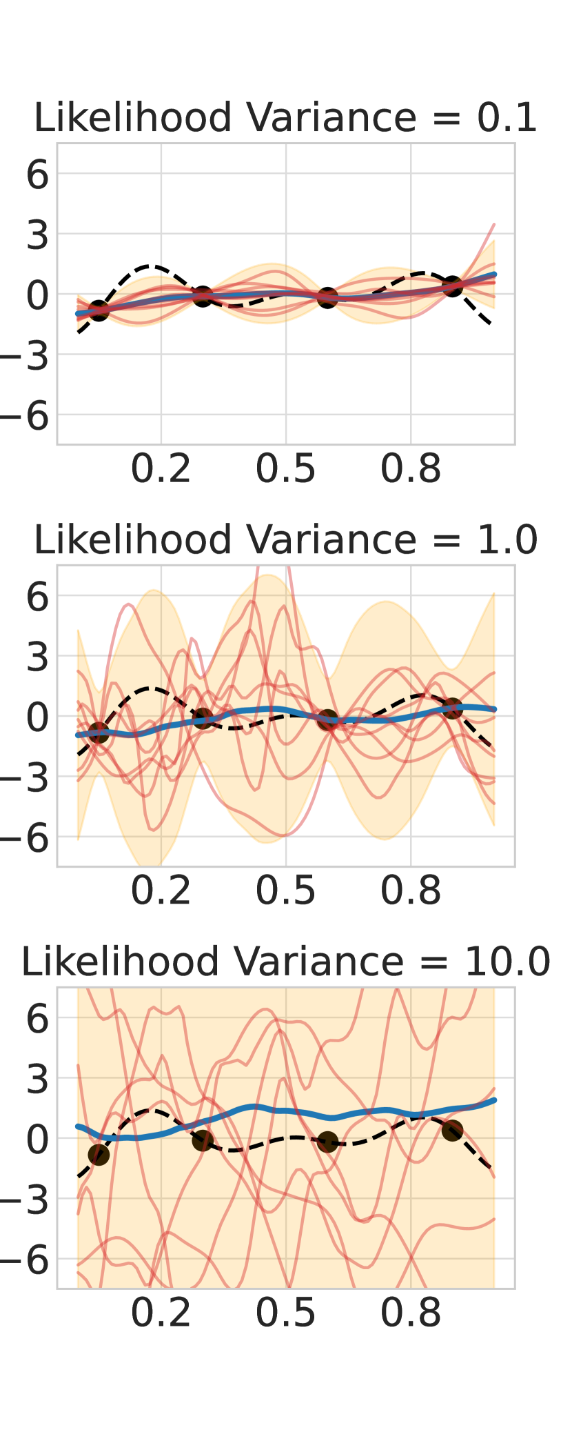
(a) Likelihood Variance

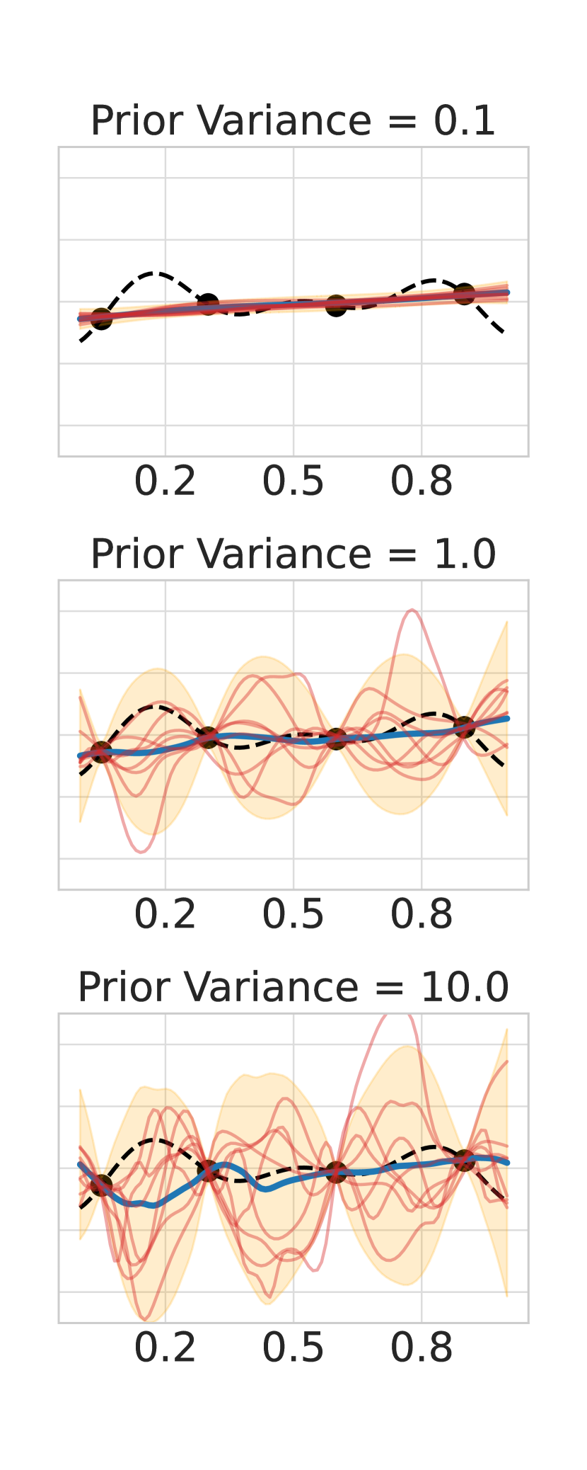
(b) Prior Variance

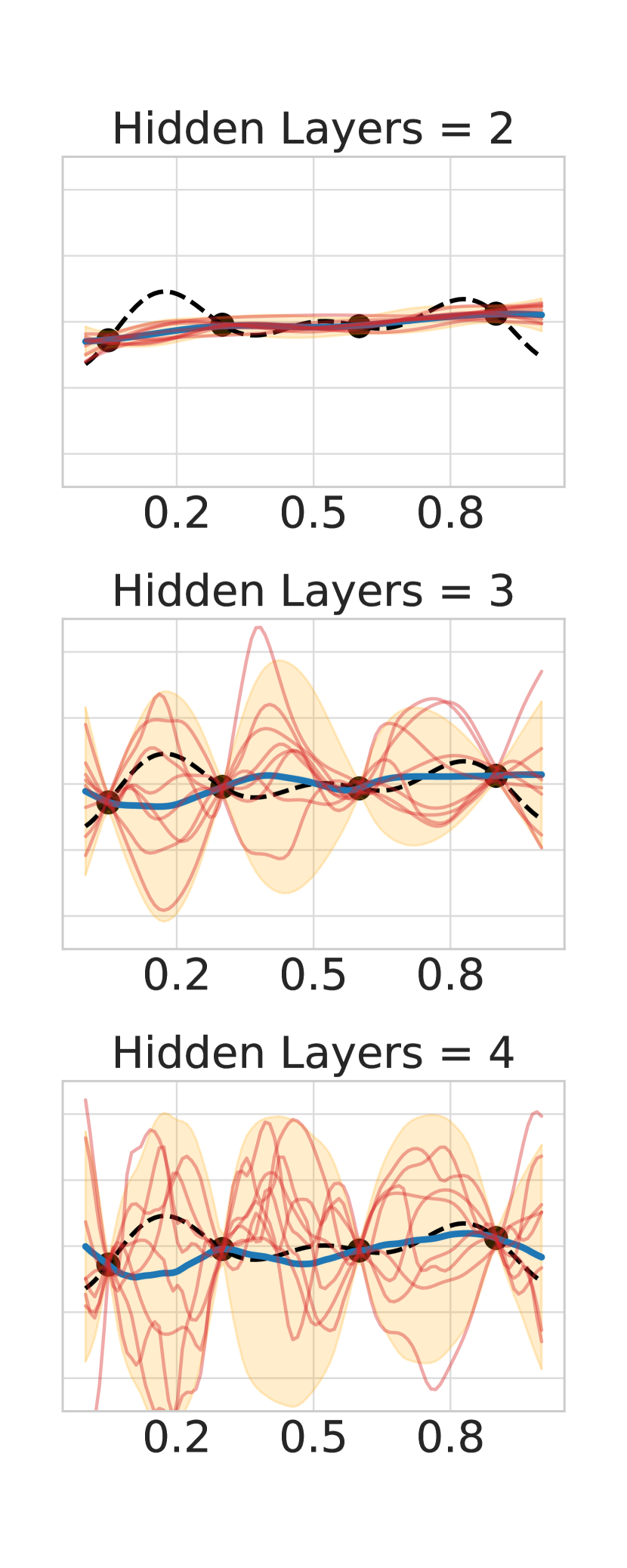
(c) Network Depth

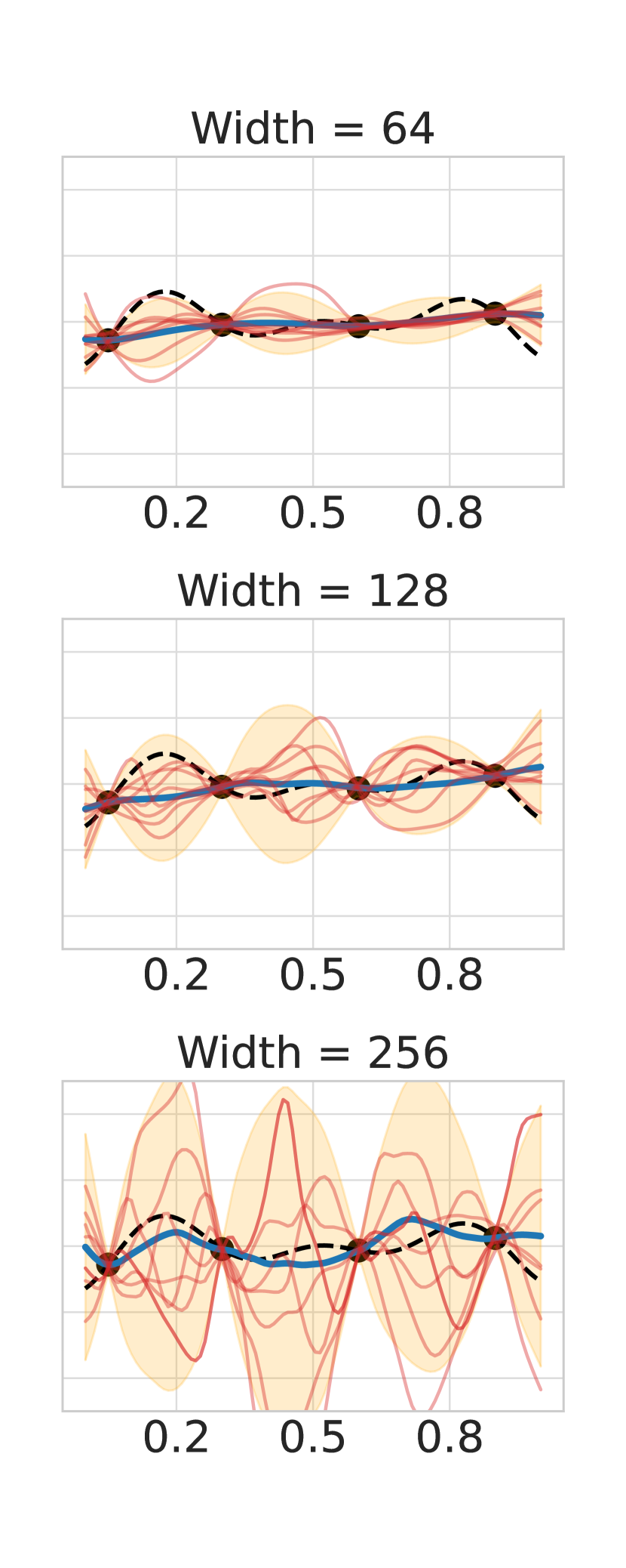
(d) Network Width

Figure 1: The design of the bnn has a significant impact on the uncertainty estimates. We visualize the uncertainty estimates and function draws produced by full-batch hmc on a simple toy objective function with four function queries (denoted in black). For the visualizations above, we fix all other design choices with the following base parameters: likelihood variance $=1$, prior variance $=1$, number of hidden layers $=3$, and width $=128$. We see that varying the different aspects of the model leads to significantly different posterior predictive distributions.

Fully Stochastic Finite-Width Bayesian Neural Networks.

These models treat all of the parameters of the neural network as random variables, which necessitates approximate inference. We consider four different mechanisms of approximate inference: (1) Hamiltonian Monte Carlo (hmc), an MCMC procedure which is the computationally expensive gold standard [15, 27, 28]; (2) Stochastic Gradient Hamiltonian Monte Carlo (sghmc), a scalable MCMC approach that works with mini-batches [3]; (3) Deep Ensembles, considered a practically effective heuristic that ensembles a neural network retrained multiple times, and has been shown to approximate fully Bayesian inference [15, 21]. These approaches are fully stochastic, and can do representation learning, meaning that they can learn appropriate distance metrics for the data as well as particular types of non-stationarity.

Deep Kernel Learning.

Deep kernel learning (dkl) [48] is a hybrid Bayesian deep learning model, which layers a GP on top of a neural network feature extractor. This approach can do non-Euclidean representation learning, handle non-stationarity, and also uses exact inference. However, it is only stochastic about the last layer.

Linearized Laplace Approximation.

The linearized-Laplace approximation (lla) is a deterministic approximate inference method that uses the Laplace approximation [24, 14] to produce a linear model from a neural network, and has recently been considered for Bayesian optimization in concurrent work [19].

Infinite-Width Bayesian Neural Networks.

Infinite-width neural networks (i-bnns) refer to the behavior of neural networks as the number of nodes per hidden layer increases to infinity. Neal [27] famously showed with a central limit theorem argument that a bnn with a single infinite-width hidden layer converges to a gp with a neural network covariance function, and this result has been extended to deep neural networks by Lee et al. [22]. i-bnns are fully stochastic and very different from standard gps, as it can handle non-stationarity and provides a non-Euclidean notion of distance inspired by a neural network. However, it cannot do representation learning and instead has a fixed covariance function that provides a relatively strong prior.

3.1 Role of Architecture

We conduct a sensitivity study into the role of architecture and other key design choices for bnn surrogate models. We highlight results for hmc inference, as it is the gold standard for approximate inference in bnns [15].

Gaussian processes involve relatively few design choices — essentially only the covariance function, which is often simply set to the RBF or Matérn kernel. Additionally, we are able to have an intuitive understanding of what the induced distributions over functions look like for the different choices of covariance functions.

In contrast, with bnns, we must consider the architecture, the prior over parameters, and the approximate inference procedure. It is also less clear how different modeling choices in bnns affect the inferred posterior predictive distributions. To illustrate these differences for varying network, prior, and variance parameters, we plot the inferred posterior predictive distributions over functions for different network widths and depths, the activation functions, and likelihood and variance parameters in Figure 1, and we evaluate the performance under different model choices for three synthetic data problems in Figure 2. We focus on fully-connected multi-layer perceptrons for this study: while certain architectures have powerful inductive biases for computer vision and language tasks, generic regression tasks such as Bayesian optimization tend to be well-suited for fully-connected multi-layer perceptrons, which have relatively mild inductive biases and make loose assumptions about the structure of the function we are modeling.

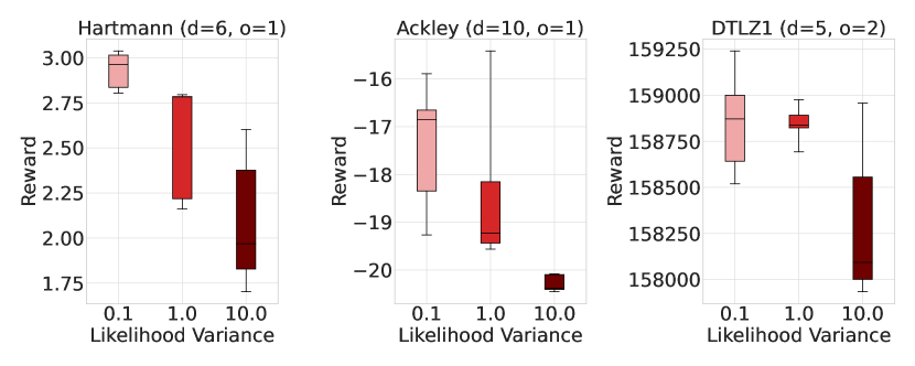
(a) Likelihood Variance

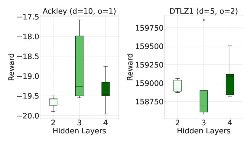
(b) Network Depth

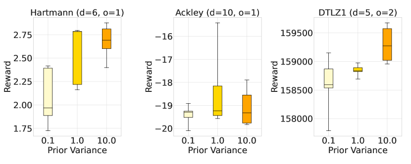
(c) Prior Variance

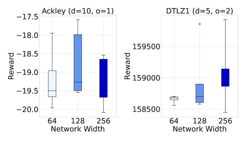
(d) Network Width

Figure 2: There is no single architecture for hmc that performs the best across all problems. We compare the impact of the design on the Bayesian optimization performance for different benchmark problems. For each set of experiments, we fix all other aspects of the design and plot the values of the maximum reward found using hmc after 100 function evaluations over 10 trials.

Model Hyperparameters.

We consider isotropic priors over the neural network parameters with zero mean and variance parameters 0.1, 1, and 10. Similarly, we consider Gaussian likelihood functions with variance parameters 0.1, 1, and 10. The corresponding posterior predictive distributions for full-batch hmc are shown in Figure 1(a). As would be expected, an increase in the likelihood variance results in a poor fit of the data and virtually no posterior collapse. In contrast, increasing the prior variance results in a higher predictive variance between data points with a good fit to the data points, whereas a prior variance that is too small leads to over-regularization and uncertainty collapse. As shown in Figure 2(a) and Figure 2(c), lower likelihood variance parameters and larger prior variance parameters tended to perform best across three synthetic data experiments.

Network Width and Depth.

To better understand the effects of the network size on inference, we explore the differences in performance when varying the number of hidden layers and the number of parameters per layer, each corresponding to an increase in model complexity. In Figure 1(c), we can see that there is a significant increase in uncertainty as we increase the number of hidden layers from two to three, and a bnn with four hidden layers has even larger uncertainty with higher variations in the function draws. Figure 1(d) also shows an increase in uncertainty as we increase the width of the network, where a smaller width leads to function draws that are much flatter than function draws from a larger width. However, the best size to choose seems to be problem-dependent, as shown in Figure 2(b) and Figure 2(d).

Activation Function.

The choice of activation function in a neural network determines important characteristics of the function class, such as smoothness or periodicity. The impact of the activation function can be seen in Appendix D, with function draws from the ReLU bnn appearing more jagged and function draws from the tanh bnn more closely resembling the draws from a gp with a Squared Exponential or Matérn 5/2 covariance function.

4 Empirical Evaluation

We provide an extensive empirical evaluation of bnn surrogates for Bayesian optimization. We first assess how bnns compare to gps in relatively simple and well-understood settings through commonly used synthetic objective functions, and we perform an empirical comparison between gps and different types of bnns (hmc, sghmc, lla, ensemble, i-bnn, and dkl). To further ascertain whether bnns may be a suitable alternative to gps in real-world Bayesian optimization problems, we study six real-world datasets used in prior work on Bayesian optimization with gp surrogates [5, 6, 25, 30, 43]. We also provide evidence that the performance of bnns could be further improved with a careful selection of network hyperparameters. We conclude our evaluation with a case study of Bayesian optimization tasks where simple Gaussian process models may fail but bnn models would be expected to prevail. To this end, we design a set of experiments to assess the performance of gps and bnns as a function of the input dimensionality and in settings where the objective function is non-stationary.

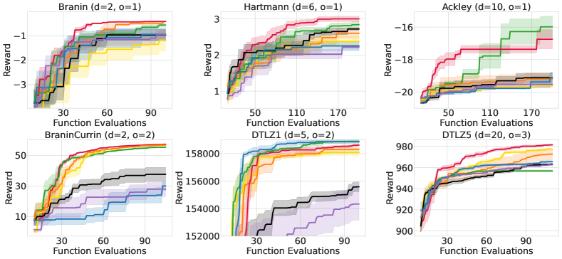
Figure 3: bnns are often comparable to gps on standard synthetic benchmarks. However, the type of bnn used has a big impact: hmc is similar to gps and even outperforms them on Ackley, while sghmc and deep ensembles seem to have less reliable performance and are often unable to effectively find the maximum. i-bnns also seem to struggle on these low-dimensional problems. For each benchmark function, we include $d$ for the number of input dimensions, and $o$ for the number of objectives. We plot the mean and one standard error of the mean over 5 trials.

4.1 Synthetic Benchmarks

We evaluate bnn and gp surrogates on a variety of synthetic benchmarks, and we choose problems with a wide span of input dimensions to understand how the performance differs as we increase the dimensionality of the data. We also select problems that vary in the number of objectives to compare the performance of the different surrogate models. Detailed problem descriptions can be found in Appendix B, and we include the experiment setup in Appendix C. We use Monte-Carlo based Expected Improvement [1] as our acquisition function for all problems.

As shown in Figure 3, we find bnn surrogate models to show promising results; however, the specific performance of different bnns varies considerably per problem. dkl matches gps in Branin and BraninCurrin, but seems to perform poorly on highly non-stationary problems such as Ackley. i-bnns also seem to slightly underperform compared to gps on these synthetic problems, many of which have a small number of input dimensions. In contrast, we find finite-width bnns using full hmc to be comparable to gps, performing very similarly in many of the experiments, slightly underperforming in Hartmann and DTLZ5, and outperforming standard gps in the 10-dimensional Ackley experiment. However, this behavior is not generalizable to all approximate inference methods: the performance of sghmc and lla vary significantly per problem, matching the performance of hmc and gps in some experiments while failing to approach the maximum value in others. Deep ensembles also consistently underperform the other surrogate models, plateauing at noticeably lower objective values on multi-objective problems like BraninCurrin and DTLZ1. This result is surprising, since ensembles are often seen to as an effective way to measure uncertainty (Appendix D).

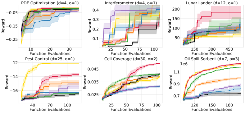
Figure 4: Real world benchmarks show mixed results. bnns outperform gps on some problems and underperform on others, and there does not seem to be a noticeable preference for any particular surrogate as we increase the number of input dimensions. Additionally, there does not appear to be a clear separation between the top row of experiments, which optimize over continuous parameters, and the bottom row of experiments, which also include some discrete inputs. For each benchmark, we include $d$ for the number of input dimensions, and $o$ for the number of objectives. We plot the mean and one standard error of the mean over 5 trials.

4.2 Real-World Benchmarks

To provide an evaluation of bnn surrogates in more realistic optimization problems, we consider a diverse selection of real-world applications which span a variety of domains, such as solving differential equations and monitoring cellular network coverage [5, 6, 25, 30, 43]. Many of these problems, such as the development of materials to clean oil spills, have consequential applications; however, these objectives are often multi-modal and are difficult to optimize globally. Additionally, unlike the synthetic benchmarks, many real-world applications consist of input data with ordinal or categorical values, which may be difficult for gps to handle. Several of the problems also require multiple objectives to be optimized. Detailed problem descriptions are provided in Appendix B.

We share the results of our experiments in Figure 4, and details about the experiment setup can be found in Appendix C. The results are mixed: bnns are able to significantly outperform gps in the Pest Control dataset, while gps find the maximum reward in the Cell Coverage and Lunar Lander experiments. The Pest Control, Cell Coverage, and Oil Spill Sorbent experiments all include discrete input parameters, and there seems to be a slight trend of gp and i-bnns performing well, and sghmc and ensembles performing more poorly. Similar to the findings from the synthetic benchmarks, we see that the different approximate inference methods for finite-width bnns lead to significantly different Bayesian optimization performance, with hmc generally finding higher rewards compared to sghmc, lla, and deep ensembles. Additionally, it appears that gps perform well in the two multi-objective problems, although that may not be generalizable to additional multi-objective problems and may be more related to the curvature of the specific problem space.

4.3 Neural Architecture Search

To better understand the impact of architecture on the performance of bnns, we conduct an extensive neural architecture search over a selection of the benchmark problems, varying the width, depth, prior variance, likelihood variance, and activation function. For our experiments, we use SMAC3 [23], a framework which uses Bayesian optimization to select the best hyperparameters, and we detail the experiment setup in Appendix C. While a thorough search over architectures is often impractical for realistic settings of Bayesian optimization since it requires a very large number of function evaluations, we use this experiment to demonstrate the flexibility of bnns and to showcase its potential when the design is well-suited for the problem.

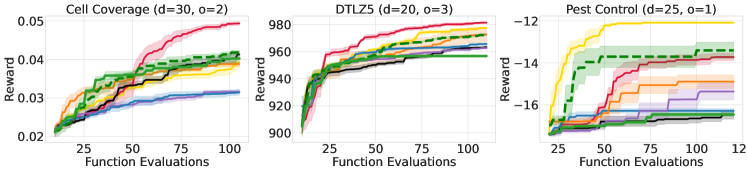
Figure 5: The impact of neural architecture search on hmc is problem-dependent. The dashed green line indicates the performance of hmc after an extensive neural architecture search, compared to the solid green line representing the hmc model selected from a much smaller pool of hyperparameters. We see that it has minimal impact on Cell Coverage (left), moderate impact on DTLZ5 (center), and extensive impact on Pest Control (right), even outperforming gps. For each benchmark, we include $d$ for the number of input dimensions, and $o$ for the number of objectives. We plot the mean and one standard error of the mean over 5 trials.

We show the effect of neural architecture search on hmc surrogate models in Figure 5. On the Cell Coverage problem, the architecture search did not drastically change the performance of hmc. In contrast, extensively optimizing the hyperparameters made a significant difference on the Pest Control problem, leading to hmc finding higher rewards than gps while using fewer function evaluations; however, on this problem i-bnn, which does not require specifying an architecture, still performs best. Neural architecture search was also able to improve the results on DTLZ5, leading hmc to be competitive with other surrogate models such as i-bnns and dkl. The difference in the benefits of the search may be attributed to some problems having less inherent structure than others, where extensive hyperparameter optimization may not be as necessary. Additionally, our original hmc surrogate model choice may already have been a suitable choice for some problems, so an extensive search over architectures may not significantly improve the performance.

4.4 Limitations of GP Surrogate Models

Although popular, gps suffer from well-known limitations that directly impact their usefulness as surrogate models. To contrast bnn and gp surrogates, we explore two failure modes of gps and demonstrate that the increased flexibility provided by bnn surrogate models can overcome these issues and improve performance in Bayesian optimization.

Non-Stationary Objective Functions.

To use gp surrogates, we must specify a kernel function class that governs the covariance structure over data points and learn the kernel hyperparameters. We typically constrain model selection to models with kernel of the form $k(\operatorname{\mathbf{x}},\operatorname{\mathbf{x}}^{\prime})=k(\lVert\operatorname{\mathbf{x}}-\operatorname{\mathbf{x}}^{\prime}\rVert)$. This constraint makes it easier to describe the functional form and learn the hyperparameters of the kernel. However, because the covariance between two values only depends on their distance and not on the values themselves, this setup assumes the function is stationary and has similar mean and smoothness throughout the input space. Unfortunately, this assumption of stationarity does not hold true in many real-world settings. For example, in the common Bayesian optimization application of choosing hyperparameters of a neural network, the true loss function landscape may have vastly different behavior in one part of the input space compared to another. bnn surrogates, in contrast to gp surrogates, are able to model non-stationary functions without similar constraints.

In Appendix D, we show the performance of Bayesian optimization with bnn and gp surrogate models for a non-stationary objective function. Because the gp assumes that the behavior of the function is the same throughout the input domain, it cannot accurately model the input-dependent variation of the function and leads to underfitting around the true optimum. In contrast, bnn surrogates can learn the non-stationarity of the function.

High-Dimensional Input Spaces.

Due to the curse of dimensionality, gps do not scale well to high-dimensional input spaces without careful human intervention. Common covariance functions may fail to faithfully represent high-dimensional input data, making the design of custom-tailored kernel functions necessary. In contrast, neural networks are well-suited for modeling high-dimensional input data [20].

To measure the effect of dimensionality on the performance of gps and bnns, we first benchmark the ability of the surrogate models to maximize synthetic test functions provided by high-dimensional polynomial functions and function draws from neural networks. To better understand the behaviors of different surrogate models in real-world settings, we also construct a high-dimensional problem by using Bayesian optimization to set the parameters of a neural network in the context of knowledge distillation. Knowledge distillation refers to the act of “distilling” information from a larger teacher model to a smaller student model by matching model outputs [11], and it is known to be a difficult optimization problem [39]. For full descriptions of the high-dimensional problems, see Appendix B.

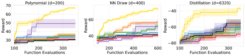
Figure 6: i-bnns outperform other surrogates in many high-dimensional settings. We show the results of maximizing a polynomial function (left), maximizing a fixed function draw from a neural network (center), and optimizing the parameters of a neural network in the context of knowledge distillation (right). All of these objectives are high-dimensional and non-stationary, and we find that bnns consistently find higher rewards than gps across all problems. We plot the mean and one standard error of the mean over 5 trials, and $d$ corresponds to the number of input dimensions.

We share the results of our findings in Figure 6 and Appendix D. There is a clear trend that i-bnns perform very well in these high-dimensional settings. The i-bnn has several conceptual advantages in this setting: (1) it provides a non-Euclidean and non-stationary similarity metric, which can be particularly valuable in high-dimensions; (2) it does not have any hyperparameters for learning, and thus is not “data hungry” — especially important in high dimensional problems with small data sizes, which provide relatively little information for representation learning.

Additionally, we find that other bnn surrogate models also outperform gps across the high-dimensional problems, providing a compelling motivation for bnns as surrogate models for Bayesian optimization.

5 Discussion

While Bayesian optimization research has made significant progress over the last few decades [10], the surrogate model is a crucial and highly underexplored design choice. Although standard gp models are the default surrogate, it is not because they have been shown to be superior to alternatives — we simply have had almost no evidence about how alternatives would perform. It is particularly timely to consider neural network surrogates, given significant recent advances in Bayesian neural networks and related approaches. The setting of Bayesian optimization is also quite different from where bnns are typically applied, involving particularly small datasets and online learning.

The fact that dkl is competitive with bnns calls into question the importance of fully stochastic surrogates — a surprising finding given the small datasets common to Bayesian optimization, where overfitting would be a more significant concern. Moreover, infinite-width bnns show promising performance in general, but especially for higher dimensional settings. Given that they also do not involve learning many hyperparameters, and do not require approximate inference, it is possible they could become a de facto standard surrogate for Bayesian optimization.

We also show that the Bayesian optimization objectives are sufficiently different such that one method does not generally dominate. This finding supports the use of simple models with strong but generic assumptions, such as standard gp models, which indeed provide relatively competitive performance. On the other hand, perhaps it is self-fulfilling that standard gps would be competitive on standard benchmarks, since most problems were designed with very few alternative models in mind. It may be time for the community to consider new benchmarks that evolve with the advances in our choice of surrogate models.

Acknowledgements

We thank Greg Benton for helpful guidance in the beginning stages of this research, and Sanyam Kapoor for discussions. This work is supported by NSF CAREER IIS-2145492, NSF I-DISRE 193471, NIH R01DA048764-01A1, NSF IIS-1910266, NSF 1922658 NRT-HDR, Meta Core Data Science, Google AI Research, BigHat Biosciences, Capital One, and an Amazon Research Award.

Code

Table of Contents

[sections] [sections]l1

Appendix A Background on Surrogate Models

A.1 Gaussian Processes

Gaussian processes (gps) [33] are distributions over functions entirely specified by a mean function $\mu(\operatorname{\mathbf{x}})$ and a covariance function $k(\operatorname{\mathbf{x}},\operatorname{\mathbf{x}}^{\prime})$. For regression tasks with gps, we assume $y(\operatorname{\mathbf{x}})=f(\operatorname{\mathbf{x}})+\epsilon$ with $f(\operatorname{\mathbf{x}})\sim\mathcal{GP}(\mu(\operatorname{\mathbf{x}}),k(\operatorname{\mathbf{x}},\operatorname{\mathbf{x}}^{\prime}))$ and $\epsilon\sim\mathcal{N}(0,\sigma^{2})$, where $\sigma^{2}$ is the likelihood variance. The functions $\mu(\operatorname{\mathbf{x}})$ and $k(\operatorname{\mathbf{x}},\operatorname{\mathbf{x}}^{\prime})$ are the mean and kernel functions of the gp that govern the functional properties and generalization performance of the model. In practice, we tune the hyperparameters of $\mu(\operatorname{\mathbf{x}})$ and $k(\operatorname{\mathbf{x}},\operatorname{\mathbf{x}}^{\prime})$ on the training data to optimize the marginal likelihood of the gp, which maximizes the probability that the gp model will have generated the data.

By the definition of a gp, for any finite collection of inputs $\mathbf{x}=[\operatorname{\mathbf{x}}_{\text{train}},\operatorname{\mathbf{x}}_{\text{test}}]$, $f(\mathbf{x})$, and thus $y(\mathbf{x})$ are jointly normal. Therefore, we can apply the rules of conditioning partitioned multivariate normals to form a posterior distribution $p\left(f(\operatorname{\mathbf{x}}_{\text{test}})\,|\,y(\operatorname{\mathbf{x}}_{\text{train}})\right)$, which will also be Gaussian.

In the context of Bayesian optimization, this simple conditioning procedure means that given some set of points at which we have already queried the objective function, we can quickly generate a posterior over potential candidate points and, with the help of an acquisition function, select the next points to query the objective.

A.2 Bayesian Neural Networks

Bayesian neural networks (bnns) are neural networks with stochastic parameters for which a posterior distribution is inferred using Bayesian inference.

More specifically, for regression tasks, we can specify a Gaussian observation model, $p(y(\operatorname{\mathbf{x}})\,|\,\operatorname{\mathbf{x}},{\bm{\theta}})=\mathcal{N}(h(\operatorname{\mathbf{x}}\,|\,{\bm{\theta}}),\sigma^{2})$, where $y(\operatorname{\mathbf{x}})$ represents a noisy observed value and $h(\operatorname{\mathbf{x}}\,|\,{\bm{\theta}})$ represents the output of a neural network with parameter realization ${\bm{\theta}}$ for input $\operatorname{\mathbf{x}}$. For bnns, a prior distribution is placed over the stochastic parameters ${\bm{\theta}}$ of the neural network, and the corresponding posterior distribution is given by $p({\bm{\theta}}\,|\,\mathcal{D})=p(\mathcal{D}\,|\,{\bm{\theta}})p({\bm{\theta}})/p(\mathcal{D})$. This posterior distribution can then be used in combination with the acquisition function for Bayesian optimization to select the next set of candidate points to query.

There are many different choices to consider when using Bayesian neural networks, such the inference method used to compute the posterior distribution, the architecture of the neural network, and the selection of which parameters are stochastic. In this work, we study the performance of five different types of bnns with varying inference methods and stochasticity.

A.2.1 Fully-Stochastic Finite-Width Neural Networks

For fully-stochastic Bayesian neural networks, every parameter of the neural network is stochastic and has a prior placed over it. Exact inference over these stochastic network parameters for fully-stochastic finite-width bnns is analytically intractable, since neural networks are non-linear in their parameters. To enable Bayesian inference in this setting, approximate inference methods can be used to find approximations to the exact posterior $p({\bm{\theta}}\,|\,\mathcal{D})$. In this work, we focus on four types of approximate inference: Hamiltonian Monte Carlo (hmc; Neal [28]), stochastic-gradient hmc [3], linearized Laplace approximations [14], and deep ensembles of deterministic neural networks [21].

Hamiltonian Monte Carlo.

Hamiltonian Monte Carlo is a Markov Chain Monte Carlo method that produces asymptotically exact samples from the posterior distribution [28] and is commonly referred to as the “gold standard” for inference in bnns. At test time, hmc approximates the integral $p(y(\operatorname{\mathbf{x}}_{\text{test}})\,|\,\mathcal{D})\approx\frac{1}{M}\sum_{i=1}^{M}p(y(\operatorname{\mathbf{x}}_{\text{test}})\,|\,{\bm{\theta}}_{i})$ using samples ${\bm{\theta}}_{i}$ drawn from the posterior over parameters.

Full-batch hmc provides the most accurate approximation of the posterior distribution but is computationally expensive and in practice limited to models with only a few hundred thousand parameters [15]. Full-batch hmc allows us to study the performance of bnns in Bayesian optimization without many of the confounding factors of inaccurate approximations of the predictive distribution.

Stochastic Gradient Hamiltonian Monte Carlo.

Stochastic gradient methods [45, 12] are commonly used as an inexpensive approach to sampling from the posterior distribution. Unlike full-batch hmc, which computes the gradients over the full dataset, stochastic gradient hmc instead samples a mini-batch to compute a noisy estimate of the gradient [3]. While these methods may seem appealing when working with large models or datasets, they can result in inaccurate approximations and posterior predictive distribution with unfaithful uncertainty representations.

Deep Ensembles.

Deep ensembles are ensembles of several deterministic neural networks, each trained using maximum a posteriori estimation using a different random seed and initialization (and sometimes using different subsets of the training data). The ensemble components can be viewed as forming an efficient approximation to the posterior predictive distribution, by choosing parameters that represent typical points in the posterior and have high functional variability [47]. Deep ensembles are easy to implement in practice and have been shown to provide highly accurate predictions and a good predictive uncertainty estimate [21, 32].

A.2.2 Fully-Stochastic Infinite-Width Neural Networks

Infinitely-wide neural networks [29] refer to the behavior of neural networks when the number of nodes in each internal layer increases to infinity. Each one of these nodes continues is stochastic and has a specific prior placed over its parameters.

Infinite-width Neural Network.

It is possible to specify a gp that has an exact equivalence to an infinitely-wide fully-connected Bayesian neural network (i-bnn) [22]. For a single-layer network, the Central Limit Theorem can be used to show that in the limit of infinite width, each output of the network will be Gaussian distributed, and the exact distribution can be computed [29, 46]. This process can then be applied recursively for additional hidden layers [22]. i-bnns can be used in the same way as gps to calculate the posterior distribution for infinitely-wide neural networks.

A.2.3 Linearized Finite-Width Neural Networks

Linearized Laplace Approximation.

The linearized Laplace approximation [14] (lla) is a deterministic approximate inference method which uses the Laplace approximation [24, 14] to produce a linear model from a neural network. llas can be represented as Gaussian processes with mean functions provided by the MAP predictive function, and covariance functions provided by the finite, empirical neural tangent kernel at the MAP estimate.

A.2.4 Partially-Stochastic Finite-Width Neural Networks

For partially-stochastic neural networks, we learn point estimates for a subset of the parameters, and we learn the full posterior distribution for the remaining parameters in the neural network.

Deep Kernel Learning.

Deep Kernel Learning (dkl) is a hybrid method that combines the flexibility of gps with the expressivity of neural networks [48]. In dkl, a neural network $g_{\mathbf{w}}(\cdot)$ parameterized by weights $\mathbf{w}$ is used to transform inputs into intermediate values, where additional gp kernels can then be applied. Specifically, given inputs $\mathbf{x}$ and a base kernel $k_{\text{BASE}}(\mathbf{x},\mathbf{x^{\prime}})$, $k_{\text{DKL}}(\mathbf{x},\mathbf{x^{\prime}})=k_{\text{BASE}}(g_{\mathbf{w}}(\mathbf{x}),g_{\mathbf{w}}(\mathbf{x^{\prime}}))$. Unlike gps with standard kernels which depend only on the distance between inputs and therefore assume that the mean and smoothness of the function are consistent throughout, dkl does not assume stationarity and is able to represent how the properties of the function change due to its neural network feature extractor.

Appendix B Problem Descriptions

B.1 Synthetic Datasets

In the single-objective case, Branin is a function with two-dimensional inputs with three global minima, Hartmann is a six-dimensional function with six local minima, and Ackley is a multi-dimensional function with many local minima which is commonly used to test optimization algorithms. We convert all problems to maximization problems, and the goal of Bayesian optimization in single-objective settings is to find the maximum value of the objective function.

For multi-objective Bayesian optimization benchmarks, BraninCurrin is a two-dimensional input and two-objective problem composed of the Branin and Currin functions, and DTLZ1 and DTLZ5 are multi-dimensional and multi-objective test functions which are used to measure an optimization algorithm’s ability to converge to the Pareto-frontier. Here, the goal is to find an input corresponding to the multi-dimensional objective value with the maximum hypervolume from a problem-specific reference point.

B.2 Real-World Datasets

Interferometer In this problem, the goal is to tune an optical interferometer through the alignment of two mirrors. We use the simulator in Sorokin et al. [37] to replicate the Bayesian optimization problem in Maddox et al. [25]. Each mirror has a continuous x and y coordinate, which should be optimized so that the two mirrors reflect light with minimal amounts of interference.

Lunar Lander Following Eriksson et al. [6], we aim to learn the parameters of a controller for a lunar lander as implemented in OpenAI gym. The controller has 12 continuous input dimensions, corresponding to events such as “change the angle of the rover if it is tilted more than $x$ degrees." The objective is to maximize the average final reward over 50 randomly generated environments.

Cellular Coverage We want to optimize the cellular network coverage and capacity from 15 cell towers [5]. Each tower has a continuous parameter corresponding to transmit power parameter and an ordinal parameter with 6 values corresponding to tilt, for a total of 15 continuous and 15 ordinal input parameters. There are two different objectives: maximize the cellular coverage, and minimize the total interference between cell towers.

Oil Spill Sorbent In this problem, we optimize the properties of a material to maximize its performance as a sorbent for marine oil spills [43]. We tune 5 ordinal parameters and 2 continuous parameters which control the manufacturing process of electrospun materials, and optimize over three objectives: water contact angle, oil absorption capacity, and mechanical strength.

Pest Control Minimizing the spread of pests while minimizing the prevention costs of treatment is an important problem with many parallels [30]. In this experiment, we define the setting as a categorical optimization problem with 25 categorical variables corresponding to stages of intervention, with 5 different values at each stage. We optimize over two objectives: minimizing the spread of pests and minimizing the cost of prevention.

PDE Optimization Here, following Maddox et al. [25], we optimize 4 continuous parameters corresponding to the diffusivity and reaction rates of a Brusselator with spatial coupling. The objective of the problem is to minimize the variance of the PDE output.

B.3 High-Dimensional Problems

Polynomial In this optimization problem, the goal is to find the maximum value of a polynomial function. For input $\mathbf{x}\in\mathbb{R}^{d}$, the objective value is calculated using $\sum_{i=1}^{d/4}\prod_{j=1}^{4}(\mathbf{x}_{i+j}-c_{i+j})$, where $c_{i}\sim\text{Normal}(0,1)$. We set the boundaries of the input space to be $[0,1]^{d}$, and this problem setup can be used for any number of dimensions $d$.

Neural Network Draw We want to find the maximum value of a function specified by a draw from a neural network. For the neural network, we use an MLP with $d$ inputs connected to 2 hidden layers of 256 nodes each with tanh activation, connected to a final layer of size 1 (unless otherwise specified). We set each parameter $w$ in the network to a value drawn from $\mathcal{N}(0,1)$. The final objective function is equivalent to the output of the neural network with the specified weights. With this setup, we can vary $d$ to alter the input dimensionality of the problem.

Knowledge Distillation The goal of knowledge distillation is to use a larger teacher model to train a smaller student model, typically done by matching the teacher and student predictive distributions. In this problem, we use Bayesian optimization to determine the optimal parameters of the student neural network by setting our objective function as the KL divergence between the teacher and student predictive distributions. Knowledge distillation is known to be a difficult optimization problem, and this is problem also has many more dimensions than typical Bayesian optimization benchmarks. For our experiment, we use the MNIST dataset, and we train a LeNet-5 for our teacher model. For our student model, we use a small CNN with the following architecture:

1. convolutional layer with 16 convolution kernels of 3x3 (ReLU activation)

2. max pool layer 2x2

3. convolutional layer with 12 convolution kernels of 3x3 (ReLU activation)

4. max pool layer 2x2

5. fully connected layer with 10 outputs

Appendix C Experiment Details

C.1 General Setup

For all datasets, we normalize input values to be between [0, 1] and standardize output values to have mean 0 and variance 1. We also use Monte-Carlo based Expected Improvement as our acquisition function.

gp: For single-objective problems, we use gps with a Matérn $5/2$ kernel, adaptive scale, a length-scale prior of Gamma$(3,6)$, and an output-scale prior of Gamma$(2.0,0.15)$, which combine with the marginal likelihood to form a posterior which we optimize for hyperparameter learning. For multi-objective problems, we use the same gp to independently model each objective.

dkl: We set up the base kernel using the same Matérn $5/2$ kernel that we use for gps. For the feature extractor, we use the same model parameters as found in our full hmc search. For multi-objective problems, we independently model each objective.

i-bnn: We use i-bnns with 3 hidden layers and the ReLU activation function. We set the variance of the weights to 10.0, and the variance of the bias to 1.3. For multi-objective problems, we independently model each objective.

hmc: We use hmc with an adaptive step size, and we do a small search over different architectures and model choices for each problem. We use MLPs for all experiments, and we first do a grid search over MLP architectures, where we run all combinations of width (64, 128, 256), and depth (2, 3, 4, 5) with the prior and likelihood variance set to 1.0. From the best performing run, we then fix the width and depth of the network and do a grid search over the prior variance (0.1, 1.0, and 10.0) and likelihood variance (0.1, 1.0, and 10.0). We model multi-objective problems by setting the number of nodes in the final layer equal to the number of objectives.

sghmc: We use sghmc with minibatch size of 5 using the same model parameters as found in our full hmc search. We model multi-objective problems by setting the number of nodes in the final layer equal to the number of objectives.

lla: We use the same model parameters as found in our hmc search. We model multi-objective problems by setting the number of nodes in the final layer equal to the number of objectives.

ensemble: We use an ensemble of 10 models, each with the same architecture as found in the hmc search. Each model is trained on a random 80% of the function evaluations. We model multi-objective problems by setting the number of nodes in the final layer equal to the number of objectives.

We run multiple trials for all experiments, where each trial starts with a different set of initial function evaluations drawn using a Sobol sampler.

C.2 Synthetic Benchmarks

Branin We ran 5 trials using batch size 5 with 10 initial points. Our bnn models used MLPs with 3 hidden layers, 128 parameters per layer, tanh activation, likelihood variance of 0.1, and prior variance of 10.0.

Hartmann We ran 5 trials using batch size 10 with 10 initial points. Our bnn models used MLPs with 3 hidden layers, 128 parameters per layer, tanh activation, likelihood variance of 0.1, and prior variance of 1.0.

Ackley We ran 5 trials using batch size 10 with 10 initial points. Our bnn models used MLPs with 3 hidden layers, 128 parameters per layer, tanh activation, likelihood variance of 0.1, and prior variance of 0.1.

BraninCurrin We ran 5 trials using batch size 10 with 10 initial points. Our bnn models used MLPs with 3 hidden layers, 128 parameters per layer, tanh activation, likelihood variance of 0.1, and prior variance of 10.0.

DTLZ1 We ran 5 trials using batch size 5 with 10 initial points. Our bnn models used MLPs with 2 hidden layers, 128 parameters per layer, tanh activation, likelihood variance of 0.1, and prior variance of 10.0.

DTLZ5 We ran 5 trials using batch size 1 with 10 initial points. Our bnn models used MLPs with 5 hidden layers, 10 parameters per layer, tanh activation, likelihood variance of 0.001, and prior variance of 10.0.

C.3 Real-World Benchmarks

PDE Optimization We ran 5 trials using batch size 1 with 5 initial points. Our bnn models used MLPs with 3 hidden layers, 128 parameters per layer, tanh activation, likelihood variance of 1.0, and prior variance of 1.0.

Interferometer We ran 10 trials using batch size 10 with 10 initial points. Our bnn models used MLPs with 5 hidden layers, 100 parameters per layer, tanh activation, likelihood variance of 10.0, and prior variance of 10.0.

Lunar Lander We ran 5 trials using batch size 50 with 50 initial points. Our bnn models used MLPs with 5 hidden layers, 100 parameters per layer, tanh activation, likelihood variance of 10.0, and prior variance of 10.0.

Pest Control We ran 5 trials using batch size 4 with 20 initial points. Our bnn models used MLPs with 5 hidden layers, 100 parameters per layer, tanh activation, likelihood variance of 10.0, and prior variance of 10.0.

Cell Coverage We ran 5 trials using batch size 5 with 10 initial points. Our bnn models used MLPs with 3 hidden layers, 128 parameters per layer, tanh activation, likelihood variance of 0.1, and prior variance of 0.1.

Oil Spill Sorbent We ran 5 trials using batch size 10 with 10 initial points. Our bnn models used MLPs with 5 hidden layers, 100 parameters per layer, tanh activation, likelihood variance of 0.1, and prior variance of 10.0.

C.4 Neural Architecture Search

We used SMAC [23] to find the optimal hyperparameters of HMC for Cell Coverage, Pest Control, and DTLZ5 benchmark problems using Bayesian optimization. For each benchmark, our new objective function was the average maximum value found for three runs of Bayesian optimization using the same problem setup as detailed above. We used the hyperparameter optimization facade in SMAC, and for each problem, we used Bayesian optimization to select 200 different HMC architectures to find the optimal combination from the following set of possible values:

• Network width: [32, 512] (continuous)

• Network depth: {1, 2, 3, 4, 5, 6} (discrete)

• Network activation: {"ReLU", "tanh"} (discrete)

• $\log_{10}$ of likelihood variance: [-3.0, 2.0] (continuous)

• $\log_{10}$ of prior variance: [-3.0, 2.0] (continuous)

We then use the optimal architecture and run the benchmark for 5 trials with the same setup as described in Section C.2 and Section C.3 to compare the results of HMC with and without neural architecture search.

For cell coverage, the final hmc model was an MLP with 5 hidden layers, 184 parameters per layer, tanh activation, likelihood variance of 26.3, and prior variance of 0.54.

For pest control, the final hmc model was an MLP with 1 hidden layer of size 321, tanh activation, likelihood variance of 0.26, and prior variance of 0.31.

For DTLZ5, the final hmc model was an MLP with 3 hidden layers, 297 parameters per layer, relu activation, likelihood variance of 0.01, and prior variance of 0.30.

C.5 High-Dimensional Experiments

Polynomial We ran 5 trials using batch size 10 with 100 initial points. Our hmc model was an MLP with 2 hidden layers, 256 parameters per layer, tanh activation, likelihood variance of 1.0, and prior variance of 10.0.

Neural Network Draw We ran 5 trials using batch size 10 with 100 initial points. Our hmc model was an MLP with 2 hidden layers, 256 parameters per layer, tanh activation, likelihood variance of 1.0, and prior variance of 10.0.

Knowledge Distillation We ran 5 trials using batch size 10 with 100 initial points. Our hmc model was an MLP with 2 hidden layers, 256 parameters per layer, tanh activation, likelihood variance of 1.0, and prior variance of 10.0.

Appendix D Further Empirical Results

D.1 Deep Ensembles

While deep ensembles often provide good accuracy and well-calibrated uncertainty estimates in other settings [21], we show they can perform relatively poorly for Bayesian optimization. For instance, when compared to other bnns on benchmark problems such as BraninCurrin and DTLZ1, the maximum reward found by deep ensembles plateaus at a lower value than other surrogate models.

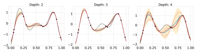
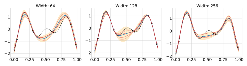
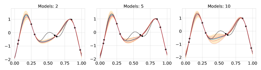
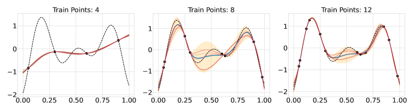
Figure A.1: We visualize the uncertainty of deep ensembles in various scenarios. For each set of experiments, we fix all other design choices with the following base parameters: depth = 3, width = 128, models = 5, train points = 9.

To further investigate the behavior of deep ensembles, we conduct a sensitivity study, varying the architecture, the amount of training data, and the number of models in the ensemble.

In Figure A.1, we see that smaller training sizes can paradoxically lead to less uncertainty with deep ensembles. A critical component in the success of deep ensembles is the diversity of its models. After training, each model falls within a distinct basin of attraction, where solutions across different basins correspond to diverse functions. Intuitively, however, in the low data regime there are fewer settings of parameters that give rise to easily discoverable basins of attraction, making it harder to find diverse solutions simply by re-initializing optimization runs. We consider, for example, the straight path between the weights of Model 1 and Model 2, and we follow how the loss changes as we linearly interpolate between the weights. Specifically, given neural network weights $\mathbf{w}_{1}$ from Model 1 and $\mathbf{w}_{2}$ from Model 2, and $\mathcal{L}(\mathbf{w})$ representing the loss of the neural network with weights $\mathbf{w}$ on the training data, we plot the loss $\mathcal{L}(\mathbf{w}_{2}+(\mathbf{w}_{1}-\mathbf{w}_{2})*x)$ for varying values of $x$.

We share results in Figure A.2 for DTLZ1, a problem where deep ensembles performed poorly. We can see that in low-data regimes, although the loss between the two models does increase, the loss is significantly higher in other regions of the loss landscape. This behavior suggests that the basins are not particularly distinct, as the loss stays relatively flat between them, and thus less likely to provide diverse solutions. However, as we increase the amount of training data, the models are able to find more pronounced basins. We also verify that the flatter regions correspond to a decrease in model diversity by measuring the cosine similarity between the model weights, and we see that in the low-data regime, models have more similar weights and therefore are less diverse.

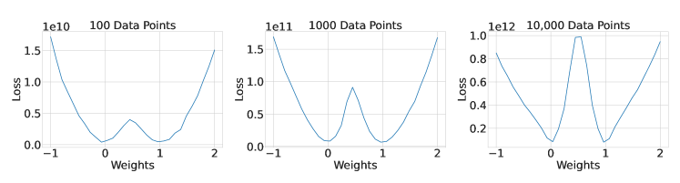
(a) Loss landscape

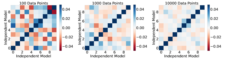
(b) Cosine similarity between models

Figure A.2: With minimal training data, the loss landscape is relatively smooth, and separately-trained models are less diverse. In the top figure, we train two models, corresponding to $x=0$ and $x=1$. We then linearly interpolate the weights between the two models to measure how the loss changes. As we increase the number of datapoints, the loss landscape becomes less smooth and models are able to find diverse basins of attraction. For the bottom figure, we train 10 models and plot the cosine similarity between weights. With less training data, the weights of the models are more related and the models are less diverse. We plot the results for DTLZ1 with 5 input dimensions and 2 output dimensions.

In general, Bayesian optimization problems contain significantly fewer datapoints than where deep ensembles are normally applied. Standard Bayesian optimization benchmarks rarely exceed about 600 data points (objective queries), while in contrast deep ensembles are often trained on problems like CIFAR-10 which have 50,000 training points.

D.2 Infinite-Width BNNs

i-bnns outperformed gps in Bayesian optimization on a variety of high-dimensional problems, and we show results in Figure A.3. The first row of results corresponds to finding the maximum value of a random polynomial function, and the second and third rows show the results of maximizing a function draw from a neural network. For the neural network function draw benchmark, we experimented with many different architectures for the neural network to ensure that we had a diverse set of objective functions to maximize, as denoted in the title of each plot. In all cases, i-bnns were able to find significantly larger values than gps.

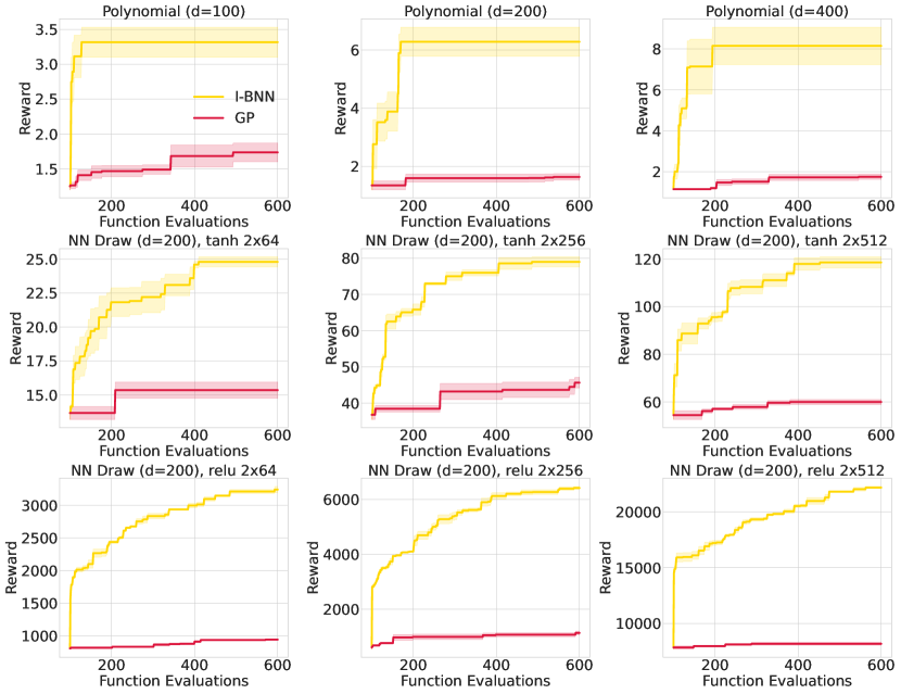
Figure A.3: i-bnns outperform gps in high dimensions. We plot the mean and one standard error of the mean over 3 trials, and $d$ corresponds to the number of input dimensions. For the neural network draw benchmark, the architecture of the neural network which the function is drawn from is also included, where $2\times 64$ means the network has 2 hidden layers of 64 nodes each.

In Figure A.4, we conduct a sensitivity analysis on the design of i-bnns, showing how the posterior changes as we vary certain hyperparameters. Unlike standard gps with RBF or Matérn kernels which are based in Euclidean similarity, i-bnns instead have a non-stationary and non-Euclidean similarity metric which is more suitable for high-dimensional problems. Additionally, i-bnns consist of a relatively strong prior, which is particularly useful in the data-scarce settings common to high-dimensional-problems.

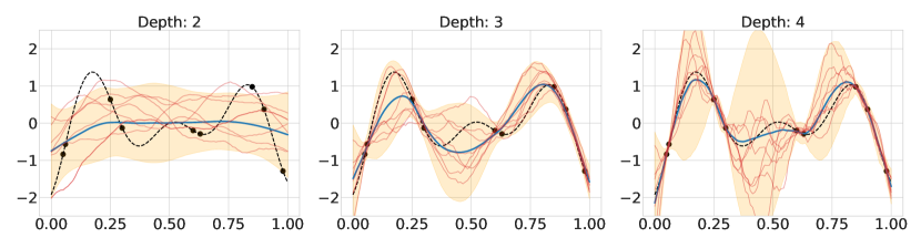
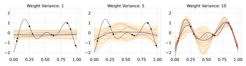
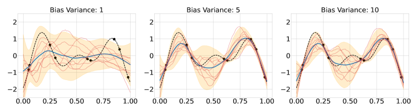
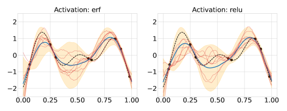
Figure A.4: We visualize how posterior predictive distribution of i-bnns changes with different design choices. For each set of experiments, we fix all other design choices with the following base parameters: depth = 3, weight variance = 10, bias variance = 5, activation = relu.

To explore the suitability of the neural network kernel, we compare the marginal likelihood of gps and i-bnns on problems with various dimensions, and we report results in Table A.1. We see that i-bnns and gps have similar marginal likelihoods on problems with fewer dimensions, such as Branin and Hartmann, but as we increase the number of dimensions, the marginal likelihood of gps becomes lower than that of i-bnns. Interestingly, we see that the marginal likelihood of gps does not decrease as quickly for Ackley as it does for the neural network draw test problem. This may be due to the neural network draw objective function having higher non-stationarity, so the standard gp kernel is less suitable for this problem compared to Ackley. For the knowledge distillation experiment, we see that the marginal likelihood of gps plummets, and it was also not able to find high rewards for the problem as shown in Figure 6. Overall, i-bnns have a higher marginal likelihood than gps on high-dimensional problems, indicating that the i-bnn prior may be more reasonable in these settings.

Problem	Dim	GP MLL	I-BNN MLL
Branin	2	-3775.3	-1354.1
Hartmann	6	-1320.4	-1630.1
Ackley	10	-1463.6	-1824.3
Ackley	20	-1657.3	-2070.2
Ackley	50	-2788.9	-2316.4
Ackley	100	-4131.6	-2456.9
NN Draw	10	-3226.9	-1829.6
NN Draw	50	-15544.3	-2344.7
NN Draw	100	-39197.5	-2453.8
NN Draw	200	-35775.2	-2584.0
NN Draw	400	-48710.9	-2737.2
NN Draw	800	-63123.4	-2868.9
Distillation	6230	-2126658.7	-3059.8

Table A.1: i-bnns have larger marginal likelihoods than gps on high-dimensional problems. Here, we show the marginal log likelihood (MLL) of gps and i-bnns on various benchmark problems, and we estimate the MLL by sampling 1000 points randomly from the input domain.

D.3 Hamiltonian Monte Carlo

We also explore the effect of the activation function on hmc. In Figure A.5, we see that the function draws from bnns with tanh activations appear quite different from the function draws from bnns with ReLU activations. The tanh draws are smoother and have more variation, while the ReLU draws seem to be more jagged. We also include results in Figure A.6 which compare the performance of ReLU and tanh activations in Bayesian optimization problems. We see that there does not appear to be an obvious trend, the optimal choice of activation function is problem-specific.

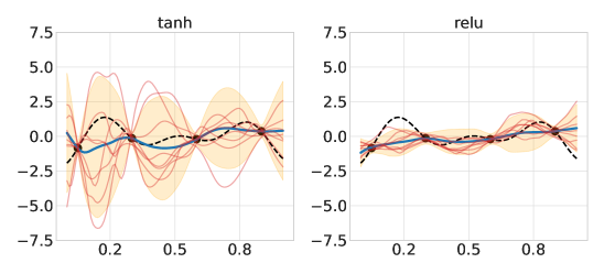
Figure A.5: The function draws of bnns with tanh activations appear to be similar to the function draws from a gp. In contrast, the function draws from bnns with ReLU are often jagged, and the network seems to deviate less from the mean.

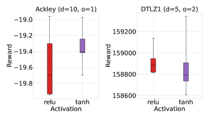
Figure A.6: In practice, ReLU and tanh activation functions can have comparable performance on synthetic functions.

D.4 Linearized Laplace Approximation

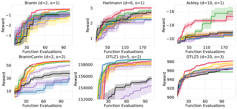
(a) Synthetic Benchmarks

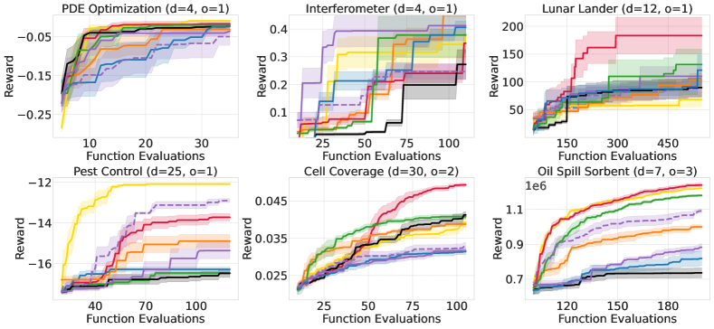
(b) Real-World Benchmarks

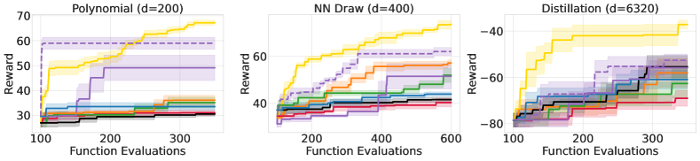
(c) High-dimensional Benchmarks

Figure A.7: The linearized Laplace approximation with a different architecture. The solid line purple line represents the performance of lla with the same architecture as the other bnn methods as specified in Appendix C, which provides a controlled comparison. The dashed purple line represents the performance of lla with the relatively small architecture specified by Kristiadi et al. [19]: an MLP with 2 hidden layers of size 50 with ReLU activation. For each benchmark, we include $d$ for the number of input dimensions, and $o$ for the number of objectives. We plot the mean and one standard error of the mean over 5 trials. Neither architecture is best for all problems, consistent with our findings in Section 3.1. While the smaller architecture tends to improve performance for lla, the i-bnn, hmc, and the standard gp generally provide stronger Bayesian optimization performance than lla.

D.5 Limitations of Gaussian Process Surrogate Models

Due to their assumptions of stationarity as noted in Section 4.4, gps struggle in non-stationary settings. In Figure A.8, we compare the posterior distribution from a gp with the posterior from different bnn surrogate models. We show results after 20 iterations of Bayesian optimization, starting with an initial point of $x=0$. The function we wish to maximize is non-stationary: the function has greater variance between $-2$ and $2$, and there is also a slight downward trend. We see that due to their stronger assumptions, gps are not able to find the true global maximum of 0.8, instead getting suck in local optima. In contrast, hmc and i-bnns are able to find the global maximum within 20 iterations.

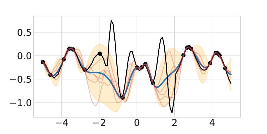
(a) gp

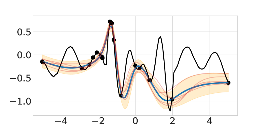
(b) hmc

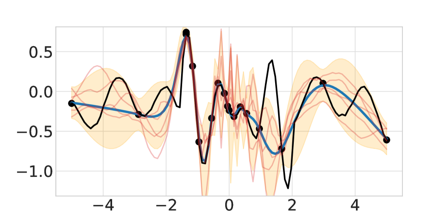
(c) i-bnn

Figure A.8: gps struggle to find the global maximum for non-stationary functions. After 20 function evaluations, the gp does not accurately model the true function around $x=-1$ because it is unable to account for the sudden increase in scale due to its assumption of stationarity. bnns do not suffer from the same pathologies and are able to find the true maximum.

An additional limitation of gp surrogate models, which we demonstrate in Figure A.9, is its performance on multi-objective problems in Bayesian optimization. Although gps have been successfully extended to a wide range of multi-objective problems, in the interest of making the approaches scalable, there are many assumptions placed onto the kernel. In the most naive setting, we can model each objective independently. While this approach is convenient, it completely ignores the relationship between objective values and has no notion of shared structure, so it is unable to take advantage of all of the information in the problem. Multi-objective covariance functions can also be decomposed as Kronecker product kernels. While this approach can have significant computational advantages compared to modeling the full covariance function, it requires each objective to itself be modeled with the same underlying kernel. Thus, this method of modeling multiple objectives will fail to capture the nuances of each particular objective when the functions have differing properties.

In Figure A.9, we show the result of twenty iterations of Bayesian optimization over a synthetic multitask example, where we care about optimizing over the fourth function but provide additional information through the other three datasets. We use the gp with Kronecker product kernels to model the multiple objectives. In our experiment, although the gp is able to learn the proper length scale and variance over the three additional functions with similar length scales, it struggles to accurately fit the fourth objective. Because the gp is unable to account for the differences between the four functions, it does not find the global optimum. Unlike gps, bnns are not restricted to strict covariance structures and are able to produce well-calibrated uncertainty estimates in multi-objective settings. The bnns are able to accurately fit all four functions, including the fourth objective function which has a much smaller length scale compared to the others.

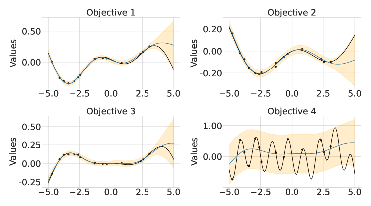
(a) gp

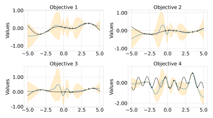
(b) hmc

Figure A.9: gps have a hard time finding the global maximum in multi-objective settings. Multi-task gps learn one length scale across all objectives, which may not be suitable for many datasets. In this example, it does not find the global minimum in the 4th objective because it treats the shorter length scale as noise. In contrast, bnns are able to appropriately model the uncertainty for the 4th objective and find its true minimum.

References

- Balandat et al. [2020] Maximilian Balandat, Brian Karrer, Daniel Jiang, Samuel Daulton, Ben Letham, Andrew G Wilson, and Eytan Bakshy. Botorch: A framework for efficient monte-carlo bayesian optimization. Advances in neural information processing systems, 33:21524–21538, 2020.
- Bergstra et al. [2013] James Bergstra, Daniel Yamins, and David Cox. Making a science of model search: Hyperparameter optimization in hundreds of dimensions for vision architectures. In International conference on machine learning, pages 115–123. PMLR, 2013.
- Chen et al. [2014] Tianqi Chen, Emily B Fox, Carlos Guestrin, and Michael I Jordan. Stochastic gradient hamiltonian monte carlo. In International Conference on Machine Learning, pages 1683–1691, 2014.
- Daxberger et al. [2021] Erik Daxberger, Agustinus Kristiadi, Alexander Immer, Runa Eschenhagen, Matthias Bauer, and Philipp Hennig. Laplace redux-effortless bayesian deep learning. Advances in Neural Information Processing Systems, 2021.
- Dreifuerst et al. [2021] Ryan M Dreifuerst, Samuel Daulton, Yuchen Qian, Paul Varkey, Maximilian Balandat, Sanjay Kasturia, Anoop Tomar, Ali Yazdan, Vish Ponnampalam, and Robert W Heath. Optimizing coverage and capacity in cellular networks using machine learning. In ICASSP 2021-2021 IEEE International Conference on Acoustics, Speech and Signal Processing (ICASSP), pages 8138–8142. IEEE, 2021.
- Eriksson et al. [2019] David Eriksson, Michael Pearce, Jacob Gardner, Ryan D Turner, and Matthias Poloczek. Scalable global optimization via local bayesian optimization. Advances in neural information processing systems, 32, 2019.
- Frazier [2018] Peter I Frazier. A tutorial on bayesian optimization. Foundations and Trends® in Machine Learning, 11(1):1–96, 2018.
- Frazier et al. [2008] Peter I Frazier, Warren B Powell, and Savas Dayanik. A knowledge-gradient policy for sequential information collection. SIAM Journal on Control and Optimization, 2008.
- Gardner et al. [2017] Jacob Gardner, Chuan Guo, Kilian Weinberger, Roman Garnett, and Roger Grosse. Discovering and exploiting additive structure for bayesian optimization. In Artificial Intelligence and Statistics, 2017.
- Garnett [2023] Roman Garnett. Bayesian optimization. Cambridge University Press, 2023.
- Hinton et al. [2015] Geoffrey Hinton, Oriol Vinyals, and Jeff Dean. Distilling the knowledge in a neural network. arXiv preprint arXiv:1503.02531, 2015.
- Hoffman et al. [2013] Matthew D. Hoffman, David M. Blei, Chong Wang, and John Paisley. Stochastic variational inference. Journal of Machine Learning Research, 14(1):1303–1347, May 2013. ISSN 1532-4435.
- Hutter et al. [2011] Frank Hutter, Holger H Hoos, and Kevin Leyton-Brown. Sequential model-based optimization for general algorithm configuration. In International conference on learning and intelligent optimization, pages 507–523. Springer, 2011.
- Immer et al. [2021] Alexander Immer, Maciej Korzepa, and Matthias Bauer. Improving predictions of bayesian neural nets via local linearization. In International Conference on Artificial Intelligence and Statistics, pages 703–711. PMLR, 2021.
- Izmailov et al. [2021] Pavel Izmailov, Sharad Vikram, Matthew D Hoffman, and Andrew Gordon Gordon Wilson. What are bayesian neural network posteriors really like? In International conference on machine learning, pages 4629–4640. PMLR, 2021.
- Kandasamy et al. [2015] Kirthevasan Kandasamy, Jeff Schneider, and Barnabás Póczos. High dimensional bayesian optimisation and bandits via additive models. In International conference on machine learning, 2015.
- Khan and Rue [2021] Mohammad Emtiyaz Khan and Håvard Rue. The bayesian learning rule. arXiv preprint arXiv:2107.04562, 2021.
- Kim et al. [2021] Samuel Kim, Peter Y Lu, Charlotte Loh, Jamie Smith, Jasper Snoek, and Marin Soljacic. Deep learning for bayesian optimization of scientific problems with high-dimensional structure. Transactions of Machine Learning Research, 2021.
- Kristiadi et al. [2023] Agustinus Kristiadi, Alexander Immer, Runa Eschenhagen, and Vincent Fortuin. Promises and pitfalls of the linearized laplace in bayesian optimization. arXiv preprint arXiv:2304.08309, 2023.
- Krizhevsky et al. [2012] Alex Krizhevsky, Ilya Sutskever, and Geoffrey E. Hinton. ImageNet classification with deep convolutional neural networks. In Advances in Neural Information Processing Systems 25:, pages 1106–1114, 2012.
- Lakshminarayanan et al. [2017] Balaji Lakshminarayanan, Alexander Pritzel, and Charles Blundell. Simple and scalable predictive uncertainty estimation using deep ensembles. Advances in neural information processing systems, 30, 2017.
- Lee et al. [2017] Jaehoon Lee, Yasaman Bahri, Roman Novak, Samuel S Schoenholz, Jeffrey Pennington, and Jascha Sohl-Dickstein. Deep neural networks as gaussian processes. arXiv preprint arXiv:1711.00165, 2017.
- Lindauer et al. [2022] Marius Lindauer, Katharina Eggensperger, Matthias Feurer, André Biedenkapp, Difan Deng, Carolin Benjamins, Tim Ruhkopf, René Sass, and Frank Hutter. Smac3: A versatile bayesian optimization package for hyperparameter optimization. Journal of Machine Learning Research, 23(54):1–9, 2022. URL http://jmlr.org/papers/v23/21-0888.html.
- MacKay [1992] David JC MacKay. A practical bayesian framework for backpropagation networks. Neural computation, 4(3):448–472, 1992.
- Maddox et al. [2021] Wesley J Maddox, Maximilian Balandat, Andrew G Wilson, and Eytan Bakshy. Bayesian optimization with high-dimensional outputs. Advances in Neural Information Processing Systems, 34:19274–19287, 2021.
- Moss et al. [2020] Henry Moss, David Leslie, Daniel Beck, Javier Gonzalez, and Paul Rayson. Boss: Bayesian optimization over string spaces. Advances in Neural Information Processing Systems, 2020.
- Neal [1996] Radford M Neal. Bayesian Learning for Neural Networks. 1996.
- Neal [2010] Radford M. Neal. MCMC using Hamiltonian dynamics. Handbook of Markov Chain Monte Carlo, 54:113–162, 2010.
- Neal and Neal [1996] Radford M Neal and Radford M Neal. Priors for infinite networks. Bayesian learning for neural networks, pages 29–53, 1996.
- Oh et al. [2019] Changyong Oh, Jakub Tomczak, Efstratios Gavves, and Max Welling. Combinatorial bayesian optimization using the graph cartesian product. Advances in Neural Information Processing Systems, 32, 2019.
- O’Hagan [1978] A O’Hagan. On curve fitting and optimal design for regression. J. Royal Stat. Soc. B, 40:1–32, 1978.
- Ovadia et al. [2019] Yaniv Ovadia, Emily Fertig, Jie Ren, Zachary Nado, D. Sculley, Sebastian Nowozin, Joshua Dillon, Balaji Lakshminarayanan, and Jasper Snoek. Can you trust your model’s uncertainty? Evaluating predictive uncertainty under dataset shift. In Advances in Neural Information Processing Systems 32. 2019.
- Rasmussen and Williams [2006] Carl Edward Rasmussen and Christopher KI Williams. Gaussian processes for machine learning, volume 2. MIT Press Cambridge, MA, 2006.
- Rudner et al. [2022] Tim G. J. Rudner, Freddie Bickford Smith, Qixuan Feng, Yee Whye Teh, and Yarin Gal. Continual Learning via Sequential Function-Space Variational Inference. In Proceedings of the 38th International Conference on Machine Learning, Proceedings of Machine Learning Research. PMLR, 2022.
- Snoek et al. [2012] Jasper Snoek, Hugo Larochelle, and Ryan P Adams. Practical bayesian optimization of machine learning algorithms. Advances in neural information processing systems, 25, 2012.
- Snoek et al. [2015] Jasper Snoek, Oren Rippel, Kevin Swersky, Ryan Kiros, Nadathur Satish, Narayanan Sundaram, Mostofa Patwary, Mr Prabhat, and Ryan Adams. Scalable bayesian optimization using deep neural networks. In International conference on machine learning, pages 2171–2180. PMLR, 2015.
- Sorokin et al. [2020] Dmitry Sorokin, Alexander Ulanov, Ekaterina Sazhina, and Alexander Lvovsky. Interferobot: aligning an optical interferometer by a reinforcement learning agent. Advances in Neural Information Processing Systems, 33:13238–13248, 2020.
- Springenberg et al. [2016] Jost Tobias Springenberg, Aaron Klein, Stefan Falkner, and Frank Hutter. Bayesian optimization with robust bayesian neural networks. Advances in neural information processing systems, 29, 2016.
- Stanton et al. [2021] Samuel Stanton, Pavel Izmailov, Polina Kirichenko, Alexander A Alemi, and Andrew G Wilson. Does knowledge distillation really work? Advances in Neural Information Processing Systems, 34:6906–6919, 2021.
- Stanton et al. [2022] Samuel Stanton, Wesley Maddox, Nate Gruver, Phillip Maffettone, Emily Delaney, Peyton Greenside, and Andrew Gordon Wilson. Accelerating Bayesian optimization for biological sequence design with denoising autoencoders. In International Conference on Machine Learning, 2022.
- Swersky et al. [2013] Kevin Swersky, Jasper Snoek, and Ryan P Adams. Multi-task bayesian optimization. Advances in neural information processing systems, 26, 2013.
- Tran et al. [2022] Dustin Tran, Jeremiah Liu, Michael W. Dusenberry, Du Phan, Mark Collier, Jie Ren, Kehang Han, Zi Wang, Zelda Mariet, Huiyi Hu, Neil Band, Tim G. J. Rudner, Karan Singhal, Zachary Nado, Joost van Amersfoort andAndreas Kirsch, Rodolphe Jenatton, Nithum Thain, Honglin Yuan, Kelly Buchanan, Kevin Murphy, D. Sculley, Yarin Gal, Zoubin Ghahramani, Jasper Snoek, and Balaji Lakshminarayanan. Plex: Towards Reliability Using Pretrained Large Model Extensions. 2022.
- Wang et al. [2020] Boqian Wang, Jiacheng Cai, Chuangui Liu, Jian Yang, and Xianting Ding. Harnessing a novel machine-learning-assisted evolutionary algorithm to co-optimize three characteristics of an electrospun oil sorbent. ACS Applied Materials & Interfaces, 12(38):42842–42849, 2020.
- Wang and Jegelka [2017] Zi Wang and Stefanie Jegelka. Max-value entropy search for efficient bayesian optimization. In International Conference on Machine Learning, pages 3627–3635. PMLR, 2017.
- Welling and Teh [2011] Max Welling and Yee W Teh. Bayesian learning via stochastic gradient langevin dynamics. In Proceedings of the 28th international conference on machine learning (ICML-11), pages 681–688, 2011.
- Williams [1996] Christopher Williams. Computing with infinite networks. Advances in neural information processing systems, 9, 1996.
- Wilson and Izmailov [2020] Andrew G Wilson and Pavel Izmailov. Bayesian deep learning and a probabilistic perspective of generalization. Advances in neural information processing systems, 33:4697–4708, 2020.
- Wilson et al. [2016] Andrew Gordon Wilson, Zhiting Hu, Ruslan Salakhutdinov, and Eric P Xing. Deep kernel learning. In Artificial intelligence and statistics, 2016.
- Wu et al. [2017] Jian Wu, Matthias Poloczek, Andrew G Wilson, and Peter Frazier. Bayesian optimization with gradients. Advances in neural information processing systems, 30, 2017.