Magnetic Lieb–Thirring inequalities on the torus

Abstract. In this paper we prove Lieb–Thirring inequalities for magnetic Schrödinger operators on the torus, where the constants in the inequalities depend on the magnetic flux.

1. Introduction

Lieb–Thirring inequalities have important applications in mathematical physics, analysis, dynamical systems, attractors, to mention a few. A current state of the art of many aspects of the theory is presented in [7].

In certain applications Lieb–Thirring inequalities are considered on a compact manifold (e. g., torus, sphere [11]). In this case one has to impose the zero mean orthogonality condition. However, in the case of a torus the corresponding constants in the Lieb–Thirring inequalities depend on the aspect ratios of the periods, for example, on the 2D torus the rate of growth of the constants is proportional to the aspect ratio.

On the other hand, on the torus $\mathbb{T}^{d}$ with arbitrary periods it is possible to obtain bounds for the Lieb–Thirring constants that are independent of the ratios of the periods, provided that we impose a stronger orthogonality condition that the functions must have zero average over the shortest period uniformly with respect to the remaining variables [10].

In this work we prove Lieb–Thirring inequalities on the torus for the magnetic Laplacian. The introduction of the magnetic potential not only removes the orthogonality condition but makes it possible to obtain bounds for the constants that are independent of the periods of the torus (more precisely, depend only on the corresponding magnetic fluxes).

In this paper, when obtaining the constant in the Lieb–Thirring inequality we use a combination of the result obtained in [8] and also adopting the proof from [7] to the case of the magnetic operator on the torus. Surprisingly both such independent estimates play important and non-interchangeable roles depending on the magnetic fluxes.

In conclusion of this brief introduction we point out that magnetic interpolation inequalities both in $\mathbb{R}^{d}$, and in the periodic case received much attention over the last years, see [3, 4, 13] and the references therein.

We now describe our main result. Let $\mathbb{T}^{d}=\mathbb{T}^{d}(L)$ be the $d$-dimensional torus with periods $L_{1},\dots,L_{d}$. Let us consider the eigenvalue problem for the magnetic Schrödinger operator $\mathcal{H}$ in $L_{2}(\mathbb{T}^{d})$:

$$\mathcal{H}\Psi=\left(i\,\nabla_{x}-\mathbf{A}(x)\right)^{2}\Psi-V(x)\Psi$$ (1.1)

$$= \sum_{j=1}^{d}(i\partial_{x_{j}}-a_{j}(x_{j}))^{2}\Psi-V(x)\Psi=-\lambda\Psi,$$

where

$$\mathbf{A}(x)=\left(a_{1}(x_{1}),\dots a_{d}(x_{d})\right)$$

is the real-valued magnetic vector potential in the “diagonal” case when $a_{j}(x)=a_{j}(x_{j})$. For each $j$ we define the magnetic flux

$$\alpha_{j}=\frac{1}{2\pi}\,\int_{0}^{L_{j}}a_{j}(x_{j})\,dx_{j}\qquad 1\leq j\leq d,$$

and assume that $\alpha_{j}\not\in\mathbb{Z}$ for all $j$. Then we have the following result.

Theorem 1.1.

Suppose that the potential $V(x)\geq 0$ and $V\in L_{\gamma+d/2}(\mathbb{T}^{d})$. Let $\gamma\geq 1$. Then the following bound holds for the $\gamma$-moments of the negative eigenvalues of operator (1.1):

$$\sum_{n}\lambda_{n}^{\gamma}\leq L_{\gamma,d}\,\int_{\mathbb{T}^{d}}V^{\gamma+d/2}(x)\,dx,$$ (1.2)

where

$$L_{\gamma,d}\leq\left(\frac{\pi}{\sqrt{3}}\right)^{d}L_{\gamma,d}^{\mathrm{cl}}\prod_{j=1}^{d}\sqrt{\mathrm{K}(\alpha_{j})}.$$ (1.3)

Here $L_{\gamma,d}^{\mathrm{cl}}$ is the semiclassical constant (3.4), and

$$\mathrm{K}(\alpha)\leq\min(\mathrm{K}_{1}(\alpha),\mathrm{K}_{2}(\alpha)).$$

The expressions for $\mathrm{K}_{1}(\alpha)$ and $\mathrm{K}_{2}(\alpha)$ are as follows:

$$\mathrm{K}_{1}(\alpha)=\mathrm{k}(\alpha)^{2},\quad\mathrm{k}(\alpha)=\left\{\begin{array}[]{ll}\frac{1}{|\sin(2\pi\alpha)|},&\hbox{$0<\alpha\,\mathrm{mod}(1)<1/4$;}\\ 1,&\hbox{$1/4\leq\alpha\,\mathrm{mod}(1)\leq 3/4$;}\\ \frac{1}{|\sin(2\pi\alpha)|},&\hbox{$3/4<\alpha\,\mathrm{mod}(1)<1$,}\end{array}\right.$$ (1.7)

$$\mathrm{K}_{2}(\alpha)=\frac{5}{3\sqrt{3}\pi}\cdot\left[\sup_{b\geq 0}b^{5/3}\sum_{k\in\mathbb{Z}}\frac{1}{(|k+\alpha|^{3}+b)^{2}}\right]^{2}\,.$$ (1.8)

In Sections 2 and 3 we consider the one dimensional case, where this theorem is proved in the equivalent dual formulation in terms of orthonormal systems in the scalar case and the matrix case, respectively. We point out that this theorem with $\mathrm{K}(\alpha)\leq\mathrm{K}_{1}(\alpha)$ was proved in [8] and the proof was based on the magnetic interpolation inequality (2.3) (whose proof is briefly recalled in Section 2). In the 1D scalar case this inequality immediately gives the result by the method of [5], while the inequality in the essential matrix case was proved in [8] (see also [2] for the starting point of this approach).

The bound for the constant $\mathrm{K}(\alpha)\leq\mathrm{K}_{2}(\alpha)$ was proved in the 1D scalar case in [9]. The proof in the matrix case is given in Theorem 3.1. Then the inequalities for orthonormal systems are equivalently reformulated in Theorem 3.2 in terms of estimates for the negative trace and for higher-order Riesz means of negative eigenvalues in Corollary 3.1. Finally, Theorem 1.1 is proved in Section 4 by using the lifting argument with respect to dimensions [12]. The fact that the magnetic potential is of the special diagonal form is crucial here.

We see in (1.7) and (1.8) that unlike $\mathrm{K}_{1}(\alpha)$, the constant $\mathrm{K}_{2}(\alpha)$ is not given in the explicit form. A computation in Section 5 shows that in the central region $|\alpha-1/2|<0.2273$ it holds that $\mathrm{K}_{2}(\alpha)<\mathrm{K}_{1}(\alpha)$, while near the end-points $\mathrm{K}_{1}(\alpha)$ is better, see Fig. 2.

2. 1D periodic case

We consider here the magnetic Lieb–Thirring inequality in the 1D periodic case. We assume that the period equals

$$L=\frac{2\pi}{\varepsilon},\quad\varepsilon>0.$$

Of course, one can use scaling and consider only the case $\varepsilon=1$, but we prefer to consider the general case in order to trace down the corresponding constants in the most explicit way.

Theorem 2.1.

Let the family of functions $\psi_{1},\dots,\psi_{N}\in H^{1}([0,L]_{\mathrm{per}})$ be orthonormal in $L^{2}([0,L]_{\mathrm{per}})$. Then

$$\int_{0}^{L}\rho(x)^{3}\,dx\leq{\mathrm{K}}(\alpha)\sum_{n=1}^{N}\int_{0}^{L}|i\psi^{\prime}_{n}(x)-a(x)\psi_{n}(x)|^{2}\,dx,$$ (2.1)

where

$$\rho(x)=\sum_{n=1}^{N}|\psi_{n}(x)|^{2}$$

and

$$\mathrm{K}(\alpha)\leq\min(\mathrm{K}_{1}(\alpha),\mathrm{K}_{2}(\alpha)).$$

Here $\alpha$ is the magnetic flux

$$\alpha:=\frac{1}{2\pi}\int_{0}^{L}a(x)\,dx,$$ (2.2)

and the constants $\mathrm{K}_{1}(\alpha)$ and $\mathrm{K}_{2}(\alpha)$ are defined in (1.7), (1.8).

Proof.

We first point out that estimate (1.7) was obtained in [8, (6.8)], where $\mathrm{k}(\alpha)$ is the constant in the 1D magnetic interpolation inequality

$$\|u\|_{\infty}^{2}\leq\mathrm{k}(\alpha)\left(\int_{0}^{L}\left|i\,u^{\prime}(x)-a(x)u(x)\right|^{2}dx\right)^{1/2}\left(\int_{0}^{L}|u(x)|^{2}dx\right)^{1/2}.$$ (2.3)

The sharp constant $\mathrm{k}(\alpha)$ (shown in Figure 2) was found in [8, (3.5)] and is given in (1.7). For the sake of completeness we briefly recall the proof of (2.3). We further assume for the moment that the magnetic potential is constant $a(x)\equiv a=\mathrm{const}$. We use the Fourier series

$$\psi(x)=\sqrt{\frac{\varepsilon}{2\pi}}\sum_{k\in\mathbb{Z}}\widehat{\psi}_{k}e^{ik\varepsilon x},\qquad\widehat{\psi}_{k}=\sqrt{\frac{\varepsilon}{2\pi}}\int_{0}^{2\pi/\varepsilon}\psi(x)e^{-ik\varepsilon x}dx.$$

We consider the self-adjoint operator

$$A(\lambda):=\left(i\frac{d}{dx}-a\right)^{2}+\lambda I$$

and its Green’s function $G_{\lambda}(x,\xi)$

$$A(\lambda)G_{\lambda}(x,\xi)=\delta(x-\xi),$$

which is found in terms of the Fourier series

$$G_{\lambda}(x,\xi)=\frac{\varepsilon}{2\pi}\sum_{n\in\mathbb{Z}}\frac{e^{in\varepsilon(x-\xi)}}{(n\varepsilon+a)^{2}+\lambda}.$$ (2.4)

On the diagonal we obtain

$$G(\lambda):=G_{\lambda}(\xi,\xi)=\frac{\varepsilon}{2\pi}\sum_{n\in\mathbb{Z}}\frac{1}{(n\varepsilon+a)^{2}+\lambda}$$

$$=\frac{1}{\varepsilon}\frac{1}{2\pi}\sum_{n\in\mathbb{Z}}\frac{1}{(n+\alpha)^{2}+\lambda/\varepsilon^{2}}$$

$$=\frac{1}{2\sqrt{\lambda}}\,\frac{\sinh(2\pi\sqrt{\lambda}/\varepsilon)}{\cosh(2\pi\sqrt{\lambda}/\varepsilon)-\cos(2\pi\alpha)}.$$

Using a general result (see Theorem 2.2 in [14] with $\theta=1/2$) we find that the sharp constant in (2.3) is as follows

$$\mathrm{k}(\alpha)=\frac{1}{\theta^{\theta}(1-\theta)^{1-\theta}}\sup_{\lambda>0}\lambda^{\theta}G(\lambda)=\sup_{\varphi>0}F(\varphi),$$

where

$$F(\varphi)=\frac{\sinh(\varphi)}{\cosh(\varphi)-\cos(2\pi\alpha)}\,,\quad\varphi=2\pi\sqrt{\lambda}/\varepsilon.$$

An elementary analysis of the dependence of the behaviour of the function $F(\varphi)$ on the parameter $\alpha=a/\varepsilon$ (see [8] for the details) gives the expression for $\mathrm{k}(\alpha)$ in (1.7).

We now consider the case of a non-constant magnetic potential $a(x)$. It this case instead of the complex exponentials we consider the orthonormal system of functions

$$\sqrt{\frac{\varepsilon}{2\pi}}\varphi_{n}(x),\quad\varphi_{n}(x)=e^{i((n+\alpha)\varepsilon x-\int_{0}^{x}a(y)dy)}$$ (2.5)

that are periodic with period $2\pi/\varepsilon$ in view of (2.2) and satisfy

$$\left(i\frac{d}{dx}-a(x)\right)\varphi_{n}(x)=-\varepsilon(n+\alpha)\varphi_{n}(x).$$

Therefore the Green’s function of the operator $A(\lambda)$ is

$$G_{\lambda}(x,\xi)=\frac{\varepsilon}{2\pi}\sum_{n\in\mathbb{Z}}\frac{e^{i(n+\alpha)\varepsilon(x-\xi)-\int_{\xi}^{x}a(y)dy}}{\varepsilon^{2}(n+\alpha)^{2}+\lambda},$$

giving the same expression for $G_{\lambda}(\xi,\xi)$ as in (2.4) and hence the same expression for $\mathrm{k}(\alpha)$ as in the case $a(x)=\mathrm{const}$.

We can now obtain inequality (2.1) with $\mathrm{K}(\alpha)\leq\mathrm{k}(\alpha)^{2}$ by the method of [5]. For an arbitrary $\xi=(\xi_{1},\dots,\xi_{N})\in\mathbb{C}^{N}$ we set $u(x)=\sum_{n=1}^{N}\xi_{n}\psi_{n}(x)$ in (2.3). Using orthonormality we obtain

$$\biggl{|}\sum_{n=1}^{N}\xi_{n}\psi_{n}(x)\biggr{|}^{4}\leq\mathrm{k}(\alpha)^{2}|\xi|^{2}\,\sum_{n,k=1}^{N}\xi_{n}\bar{\xi}_{k}\bigl{(}i\psi^{\prime}_{n}-a\psi_{n},i\psi^{\prime}_{k}-a\psi_{k}\bigr{)}$$

For a fixed $x$ we set $\xi_{j}:=\bar{\psi}_{j}(x)$, $j=1,\dots,N$, which gives

$$\rho(x)^{3}\leq\mathrm{k}(\alpha)^{2}\sum_{n,k=1}^{N}\psi(x)_{n}\bar{\psi}_{k}(x)\bigl{(}i\psi^{\prime}_{n}-a\psi_{n},i\psi^{\prime}_{k}-a\psi_{k}\bigr{)}.$$

Integrating in $x$ and again using orthonormality we obtain (2.1) with (1.7).

It now remains to prove (1.8): $\mathrm{K}(\alpha)\leq\mathrm{K}_{2}(\alpha)$. Let $f$ be a non-negative function on $\mathbb{R}^{+}$ with $\int_{0}^{\infty}f(t)^{2}dt=1$ so that

$$\int_{0}^{\infty}f(t/E)^{2}dt=E.$$

Let $a(x)\neq\mathrm{const}$. We use the Fourier series with respect to system (2.5):

$$\psi(x)=\sqrt{\frac{\varepsilon}{2\pi}}\sum_{k\in\mathbb{Z}}\widehat{\psi}_{k}\varphi_{k}(x),\qquad\widehat{\psi}_{k}=\sqrt{\frac{\varepsilon}{2\pi}}\int_{0}^{2\pi/\varepsilon}\psi(x)\varphi_{k}(-x)dx.$$

Then we obtain that

$$\int_{0}^{L}|i\psi^{\prime}(x)-a(x)\,\psi(x)|^{2}\,dx=\sum_{k\in\mathbb{Z}}\varepsilon^{2}|k+\alpha|^{2}|\widehat{\psi}(k)|^{2}=$$

$$\int_{0}^{\infty}\sum_{k\in\mathbb{Z}}f\biggl{(}\frac{E}{\varepsilon^{2}|k+\alpha|^{2}}\biggr{)}^{2}|\widehat{\psi}_{k}|^{2}dE=\int_{0}^{L}\int_{0}^{\infty}|\psi^{E}(x)|^{2}dEdx,$$

where

$$\psi^{E}(x)=\sqrt{\frac{\varepsilon}{2\pi}}\sum_{k\in\mathbb{Z}}f\biggl{(}\frac{E}{\varepsilon^{2}|k+\alpha|^{2}}\biggr{)}\widehat{\psi}_{k}\varphi_{k}(x).$$

Therefore

$$\psi(x)-\psi^{E}(x)$$ (2.6)

$$= \sqrt{\frac{\varepsilon}{2\pi}}\sum_{k\in\mathbb{Z}}\left(1-f\biggl{(}\frac{E}{\varepsilon^{2}|k+\alpha|^{2}}\biggr{)}\right)\widehat{\psi}_{k}\varphi_{k}(x)=(\psi(\cdot),\chi^{E}(\cdot,x)),$$

where

$$\chi^{E}(x^{\prime},x)=\sqrt{\frac{\varepsilon}{2\pi}}\sum_{k\in\mathbb{Z}}\left(1-f\biggl{(}\frac{E}{\varepsilon^{2}|k+\alpha|^{2}}\biggr{)}\right)\varphi_{k}(x^{\prime})\varphi_{k}(-x).$$ (2.7)

For any $\delta>0$ we have

$$\rho(x)\leq(1+\delta)\sum_{n=1}^{N}|\psi_{n}^{E}(x)|^{2}+(1+\delta^{-1})\sum_{n=1}^{N}|\psi_{n}(x)-\psi_{n}^{E}(x)|^{2}.$$ (2.8)

In view of orthonormality, Bessel’s inequality, (2.6) and the fact that $|\varphi_{k}(x)|\equiv 1$ we have

$$\sum_{n=1}^{N}|\psi_{n}(x)-\psi_{n}^{E}(x)|^{2}=\sum_{n=1}^{N}|(\psi_{n}(\cdot),\chi^{E}(\cdot,x))|^{2}\leq$$ (2.9)

$$\leq\|\chi^{E}(\cdot,x))\|^{2}_{L^{2}(0,L)}=\frac{\varepsilon}{2\pi}\sum_{k\in\mathbb{Z}}\left(1-f\biggl{(}\frac{E}{\varepsilon^{2}|k+\alpha|^{2}}\biggr{)}\right)^{2}.$$

Next, following [6, 7] (see Remark 2.1) we set

$$f(t)=\frac{1}{1+\mu t^{3/2}},\qquad\mu=\left(\frac{4\pi}{9\sqrt{3}}\right)^{3/2}\,.$$ (2.10)

This gives

$$\|\chi^{E}(\cdot,x))\|^{2}=\frac{1}{2\pi}\varepsilon\mu^{2}E^{3}\sum_{k\in\mathbb{Z}}\frac{1}{(\varepsilon^{3}|k+\alpha|^{3}+\mu E^{3/2})^{2}}=$$ (2.11)

$$=\frac{1}{2\pi}\varepsilon^{-5}\mu^{2}\sqrt{E}E^{5/2}\sum_{k\in\mathbb{Z}}\frac{1}{(|k+\alpha|^{3}+\mu(\sqrt{E}/\varepsilon)^{3})^{2}}=$$

$$=\frac{1}{2\pi}\mu^{1/3}\sqrt{E}\cdot b^{5/3}\sum_{k\in\mathbb{Z}}\frac{1}{(|k+\alpha|^{3}+b)^{2}}\leq$$

$$\leq\frac{1}{2\pi}\mu^{1/3}\sqrt{E}\cdot\sup_{b\geq 0}b^{5/3}\sum_{k\in\mathbb{Z}}\frac{1}{(|k+\alpha|^{3}+b)^{2}}=$$

$$=\frac{1}{3^{5/4}\pi^{1/2}}\sqrt{E}\cdot\sup_{b\geq 0}b^{5/3}\sum_{k\in\mathbb{Z}}\frac{1}{(|k+\alpha|^{3}+b)^{2}}=:A(\alpha)\sqrt{E},$$

where

$$A(\alpha)=\frac{1}{3^{5/4}\pi^{1/2}}\cdot\sup_{b\geq 0}b^{5/3}\sum_{k\in\mathbb{Z}}\frac{1}{(|k+\alpha|^{3}+b)^{2}},$$

and where we singled out the factor $\sqrt{E}$, set $b:=\mu E^{3/2}/\varepsilon^{3}$, and recalled the definition of $\mu$.

Substituting this into (2.8) and optimizing with respect to $\delta$ we obtain

$$\rho(x)\leq\left(\sqrt{\sum_{n=1}^{N}|\psi^{E}_{n}(x)|^{2}}+\sqrt{A(\alpha)}E^{1/4}\right)^{2},$$

which gives that

$$\sum_{j=1}^{N}|\psi^{E}_{j}(x)|^{2}\geq\left(\sqrt{\rho(x)}-\sqrt{A(\alpha)}E^{1/4}\right)^{2}_{+}.$$

Finally,

$$\int_{0}^{L}|i\psi^{\prime}(x)-a(x)\psi(x)|^{2}\,dx=\int_{0}^{L}\int_{0}^{\infty}|\psi^{E}(x)|^{2}dEdx\geq$$

$$\geq\int_{0}^{L}\int_{0}^{\infty}\left(\sqrt{\rho(x)}-\sqrt{A(\alpha)}E^{1/4}\right)^{2}_{+}dEdx=\frac{1}{15A(\alpha)^{2}}\int_{0}^{L}\rho(x)^{3}dx.$$

The proof is complete. ∎

Remark 2.1.

The series over $k\in\mathbb{Z}$ in (2.9), which we obviously want to minimize under the condition $\int_{0}^{\infty}f(t)^{2}dt=1$, corresponds (after the change of variable $t\to\ t^{-1/2}$) to the integral

$$\int_{0}^{\infty}(1-f(t))^{2}t^{-3/2}dt.$$

A more general problem

$$\int_{0}^{\infty}(1-f(t))^{2}t^{-\beta}dt\to\inf$$

subject to the same condition $\int_{0}^{\infty}f(t)^{2}dt=1$ was solved in [6]:

$$f(t)=\frac{1}{1+\mu t^{\beta}},\qquad\mu=\left(\frac{\beta-1}{\beta}\cdot\frac{\pi/\beta}{\sin(\pi/\beta)}\right)^{\beta},\ \ \beta>1.$$ (2.12)

This explains the choice of $f(t)$ in (2.10).

3. 1D periodic case for matrices

Let $\{\bm{\psi}_{n}\}_{n=1}^{N}$ be an orthonormal family of vector-functions

$$\bm{\psi}_{n}(x)=(\psi_{n}(x,1),\dots,\psi_{n}(x,M))^{T},\quad\bm{\psi}_{n}:[0,L]_{\mathrm{per}}\to\mathbb{C}^{M}$$

and

$$(\bm{\psi}_{n},\bm{\psi}_{m}):=(\bm{\psi}_{n},\bm{\psi}_{m})_{L^{2}([0,L],\mathbb{C}^{M})}$$

$$= \sum_{j=1}^{M}\int_{0}^{L}\psi_{n}(x,j)\overline{\psi_{m}(x,j)}dx=\int_{0}^{L}\bm{\psi}_{n}(x)^{T}\overline{\bm{\psi}_{m}(x)}dx=\delta_{nm}.$$

We consider the $M\times M$ matrix $U(x)$

$$U(x)=\sum_{n=1}^{N}\bm{\psi}_{n}(x)\overline{\bm{\psi}_{n}(x)}^{T}.$$

Theorem 3.1.

The following inequality holds

$$\int_{0}^{L}{\rm Tr\,}[U(x)^{3}]dx\leq\mathrm{K}(\alpha)\sum_{n=1}^{N}\int_{0}^{L}|i\bm{\psi}^{\prime}_{n}(x)-a(x)\bm{\psi}_{n}(x)|^{2}_{\mathbb{C}^{M}}dx,$$ (3.1)

where $\mathrm{K}(\alpha)$ is defined in Theorem 1.1.

Proof.

We first show that $\mathrm{K}(\alpha)\leq\mathrm{K}_{2}(\alpha)$.

As before, let $f$ be a scalar function with $\int_{0}^{\infty}(t)^{2}dt=1$. Then

$$\int_{0}^{L}|i\bm{\psi}^{\prime}(x)-a(x)\bm{\psi}(x)|_{\mathbb{C}^{M}}^{2}\,dx=\sum_{k\in\mathbb{Z}}\varepsilon^{2}|k+\alpha|^{2}|\widehat{\bm{\psi}}(k)|^{2}_{\mathbb{C}^{M}}=$$

$$\int_{0}^{\infty}\sum_{k\in\mathbb{Z}}f\biggl{(}\frac{E}{\varepsilon^{2}|k+\alpha|^{2}}\biggr{)}^{2}|\widehat{\bm{\psi}}_{k}|^{2}_{\mathbb{C}^{M}}dE=\int_{0}^{L}\int_{0}^{\infty}|\bm{\psi}^{E}(x)|_{\mathbb{C}^{M}}^{2}dEdx,$$

where

$$\bm{\psi}^{E}(x)=\sqrt{\frac{\varepsilon}{2\pi}}\sum_{k\in\mathbb{Z}}f\left(\frac{E}{\varepsilon^{2}|k-\alpha|}\right)\varphi_{k}(x)\widehat{\bm{\psi}}_{k},\ \widehat{\bm{\psi}}_{k}=(\widehat{\psi}_{k}(1),\dots,\widehat{\psi}_{k}(M))^{T}.$$

Let $\mathbf{e}\in\mathbb{C}^{M}$ be a constant vector. Then

$$\langle U(x)\mathbf{e},\mathbf{e}\rangle=\sum_{n=1}^{N}|\mathbf{e}^{T}\bm{\psi}_{n}(x)|^{2}=\sum_{n=1}^{N}|\langle\bm{\psi}_{n}(x),\mathbf{e}\rangle|^{2}$$

$$=\sum_{n=1}^{N}|\langle\bm{\psi}_{n}(x)-\bm{\psi}_{n}^{E}(x),\mathbf{e}\rangle+\langle\bm{\psi}_{n}^{E}(x),\mathbf{e}\rangle|^{2}$$

$$\leq(1+\delta)\sum_{n=1}^{N}|\langle\bm{\psi}_{n}(x)-\bm{\psi}_{n}^{E}(x),\mathbf{e}\rangle|^{2}+(1+\delta^{-1})\sum_{n=1}^{N}|\langle\bm{\psi}_{n}^{E}(x),\mathbf{e}\rangle|^{2}$$

where $\langle\cdot,\cdot\rangle$ denotes the scalar product in $\mathbb{C}^{M}$. For the first term we have

$$\langle\bm{\psi}(x)-\bm{\psi}^{E}(x),\mathbf{e}\rangle$$

$$=\sqrt{\frac{\varepsilon}{2\pi}}\sum_{k\in\mathbb{Z}}\left(1-f\left(\frac{E}{\varepsilon^{2}|k-\alpha|^{2}}\right)\right)\varphi_{k}(x)\langle\widehat{\bm{\psi}}_{k},\mathbf{e}\rangle$$

$$=(\bm{\psi}(\cdot),\chi^{E}(\cdot,x)\mathbf{e})_{L^{2}(L,\mathbb{C}^{M})},$$

where the scalar function $\chi^{E}(x^{\prime},x)$ is as in (2.7). Now, again by orthonormality, Bessel’s inequality and (2.11) we obtain

$$\sum_{n=1}^{N}|\langle\bm{\psi}_{n}(x)-\bm{\psi}_{n}^{E}(x),\mathbf{e}\rangle|^{2}=\sum_{n=1}^{N}(\bm{\psi}_{n}(\cdot),\chi^{E}(\cdot,x)\mathbf{e})_{L^{2}(L,\mathbb{C}^{M})}$$

$$\leq\|\chi^{E}(\cdot,x)\mathbf{e}\|^{2}_{L^{2}(L,\mathbb{C}^{M})}=\|\chi^{E}(\cdot,x)\|^{2}_{L^{2}}\|\mathbf{e}\|_{\mathbb{C}^{M}}^{2}\leq A(\alpha)\sqrt{E}\|\mathbf{e}\|_{\mathbb{C}^{M}}^{2}.$$

For the second term we simply write

$$\sum_{n=1}^{N}|\langle\bm{\psi}_{n}(x),\mathbf{e}\rangle|^{2}=\langle U^{E}(x)\mathbf{e},\mathbf{e}\rangle,\quad U^{E}(x)=\sum_{n=1}^{N}\bm{\psi}^{E}_{n}(x)\overline{\bm{\psi}^{E}_{n}(x)}^{T}.$$

Combining the above we obtain

$$\langle U(x)\mathbf{e},\mathbf{e}\rangle\leq(1+\delta^{-1})\langle U^{E}(x)\mathbf{e},\mathbf{e}\rangle+(1+\delta)A(\alpha)\sqrt{E}\|\mathbf{e}\|_{\mathbb{C}^{M}}^{2}.$$

If we denote by $\lambda_{j}(x)$ and $\lambda_{j}^{E}(x)$, $j=1,\dots,M$ the eigenvalues of the (Hermitian) matrices $U(x)$ and $U^{E}(x)$, respectively, then the variational principle implies that

$$\lambda_{j}(x)\leq(1+\delta^{-1})\lambda_{j}^{E}(x)+(1+\delta)A(\alpha)\sqrt{E}.$$

Optimizing with respect to $\delta$ we find that

$$\lambda_{j}(x)\leq\left(\sqrt{\lambda_{j}^{E}(x)}+A(\alpha)^{1/2}E^{1/4}\right)^{2},$$

or

$$\lambda_{j}^{E}(x)\geq\left(\sqrt{\lambda_{j}(x)}-A(\alpha)^{1/2}E^{1/4}\right)^{2}_{+},\quad j=1,\dots,M.$$

Therefore

$$\sum_{n=1}^{N}|\bm{\psi}_{n}^{E}(x)|^{2}_{\mathbb{C}^{M}}={\rm Tr\,}_{\mathbb{C}^{M}}U^{E}(x)\geq\sum_{j=1}^{M}\left(\sqrt{\lambda_{j}(x)}-A(\alpha)^{1/2}E^{1/4}\right)^{2}_{+}.$$

Integration with respect to $E$ gives that

$$\sum_{n=1}^{N}\int_{0}^{\infty}|\bm{\psi}_{n}^{E}(x)|^{2}_{\mathbb{C}^{M}}dE\geq\sum_{j=1}^{M}\int_{0}^{\infty}\left(\sqrt{\lambda_{j}(x)}-A(\alpha)^{1/2}E^{1/4}\right)^{2}_{+}dE$$

$$= \frac{1}{15A(\alpha)^{2}}\sum_{j=1}^{M}\lambda_{j}(x)^{3}=\frac{1}{15A(\alpha)^{2}}{\rm Tr\,}U(x)^{3},$$

and integration with respect to $x$ gives (3.1) with (1.8).

We finally point out that matrix inequality (3.1) with estimate of the constant (1.7) was previously proved in [8, Theorem 6.2]. The proof given there holds formally for the case of a constant magnetic potential. However, if $a(x)\neq\mathrm{const}$ we only have to use the orthonormal family (2.5) as we have done in the proof of the scalar Lieb–Thirring inequality in Theorem 2.1. The proof is complete. ∎

It is well known [2, 7] that inequalities for orthonormal systems are equivalent to the estimates for the negative trace of the corresponding Schrödinger operator. In our case we consider the magnetic Schrödinger operator

$$H=\left(i\frac{d}{dx}-a(x)\right)^{2}-V$$ (3.2)

in $L_{2}([0,L]_{\mathrm{per}})$ with matrix-valued potential $V$.

Theorem 3.2.

Let $V(x)\geq 0$ be an $M\times M$ Hermitian matrix such that ${\rm Tr\,}V^{3/2}\in L^{1}(0,L)$. Then the spectrum of operator (3.2) is discrete and the negative eigenvalues $-\lambda_{n}\leq 0$ satisfy the estimate

$$\sum_{n}\lambda_{n}\leq\frac{2}{3\sqrt{3}}\sqrt{\mathrm{K}(\alpha)}\int_{0}^{L}{\rm Tr\,}[V(x)^{3/2}]dx$$ (3.3)

$$=\frac{\pi}{\sqrt{3}}\sqrt{\mathrm{K}(\alpha)}L_{1,1}^{\mathrm{cl}}\int_{0}^{L}{\rm Tr\,}[V(x)^{3/2}]dx,$$

where

$$L_{\gamma,d}^{\mathrm{cl}}=\frac{1}{(2\pi)^{d}}\,\int_{\mathbb{R}^{d}}(1-|\xi|^{2})_{+}^{\gamma}\,d\xi=\frac{\Gamma(\gamma+1)}{2^{d}\pi^{d/2}\Gamma(\gamma+d/2+1)}.$$ (3.4)

Proof.

Let $\{\bm{\psi}_{n}\}_{n=1}^{N}$ be the orthonormal vector valued eigenfunctions corresponding to $\{-\lambda_{n}\}_{n=1}^{N}$:

$$\left(i\frac{d}{dx}-a(x)\right)^{2}\bm{\psi}_{n}-V\bm{\psi}_{n}=-\lambda_{n}\bm{\psi}_{n}.$$

Taking the scalar product with $\bm{\psi}_{n}$, using inequality (3.1), Hölder’s inequality for traces and setting $X=\int_{0}^{L}{\rm Tr\,}[U(x)^{3}]dx$, we obtain

$$\sum_{n=1}^{N}\lambda_{n}=-\sum_{n=1}^{N}\int_{0}^{L}|(i\bm{\psi}^{\prime}(x)-a(x)\bm{\psi}_{n}(x)|^{2}_{\mathbb{C}^{M}}dx+\int_{0}^{L}{\rm Tr\,}[V(x)U(x)]dx$$

$$\leq-\mathrm{K}(\alpha)^{-1}X+\left(\int_{0}^{L}{\rm Tr\,}[V(x)^{3/2}]dx\right)^{2/3}X^{1/3}.$$

Calculating the maximum with respect to $X$ we obtain (3.3). ∎

The higher-order Riesz means of the eigenvalues for magnetic Schrödinger operators with matrix-valued potentials are obtained by the Aizenmann–Lieb argument [1, 7].

Corollary 3.1.

Let $V\geq 0$ be a $M\times M$ Hermitian matrix, such that ${\rm Tr\,}V^{\gamma+1/2}\in L_{1}(0,L)$. Then for any $\gamma\geq 1$ the negative eigenvalues of the operator (3.2) satisfy the inequalities

$$\sum\lambda_{n}^{\gamma}\leq L_{\gamma,1}\int_{0}^{L}{\rm Tr\,}[V(x)^{1/2+\gamma}]\,dx,$$ (3.5)

where

$$L_{\gamma,1}\leq\frac{2}{3\sqrt{3}}\sqrt{\mathrm{K}(\alpha)}\,\frac{L_{\gamma,1}^{\mathrm{cl}}}{L_{1,1}^{\mathrm{cl}}}=\frac{\pi}{\sqrt{3}}\sqrt{\mathrm{K}(\alpha)}\,L_{\gamma,1}^{\mathrm{cl}}.$$

4. Magnetic Schrödinger operator on the torus

Proof of Theorem 1.1.

We use the lifting argument with respect to dimensions developed in [12]. More precisely, we apply estimate (3.5) $d-1$ times with respect to variables $x_{1},\dots,x_{d-1}$ (in the matrix case), so that $\gamma$ is increased by $1/2$ at each step, and, finally, we use (3.5) (in the scalar case) with respect to $x_{d}$. Using the variational principle and denoting the negative parts of the operators by $[\,\cdot\,]_{-}$ we obtain

$$\sum_{n}\lambda_{n}^{\gamma}(\mathcal{H})=\sum_{n}\lambda_{n}^{\gamma}\biggl{(}(i\partial_{x_{1}}-a_{1}(x_{1}))^{2}+\sum_{j=2}^{d-1}(i\partial_{x_{j}}-a_{j}(x_{j}))^{2}-V(x)\biggr{)}$$

$$\ \ \leq\sum_{n}\lambda_{n}^{\gamma}\biggl{(}(i\partial_{x_{1}}-a_{1}(x_{1}))^{2}-\biggl{[}\sum_{j=2}^{d-1}(i\partial_{x_{j}}-a_{j}(x_{j}))^{2}-V(x)\biggr{]}_{-}\biggr{)}$$

$$\ \ \leq\frac{\pi}{\sqrt{3}}\sqrt{\mathrm{K}_{1}(\alpha_{1})}{L}^{\mathrm{cl}}_{\gamma,1}\int_{0}^{L_{1}}\biggl{[}(i\partial_{x_{j}}-a_{j}(x_{j}))^{2}-V(x)\biggr{]}_{-}^{\gamma+1/2}\!dx_{1}$$

$$\ \ \leq\dotsb\dotsb\dotsb\ \leq\biggl{(}\frac{\pi}{\sqrt{3}}\biggr{)}^{d-1}\ \prod_{j=1}^{d-1}\sqrt{\mathrm{K}(\alpha_{j})}\prod_{j=1}^{d-1}{L}^{\mathrm{cl}}_{\gamma+(j-1)/2,1}\times$$

$$\ \times\int_{0}^{L_{1}}\dotsi\int_{0}^{L_{d-1}}\operatorname{Tr}\bigl{[}(i\partial_{x_{d}}-a_{d}(x_{d}))^{2}-V(x)\bigr{]}_{-}^{\gamma+(d-1)/2}\,dx_{1}\dots dx_{d-1}$$

$$\ \ \leq\biggl{(}\frac{\pi}{\sqrt{3}}\biggr{)}^{d}\ \prod_{j=1}^{d}\sqrt{\mathrm{K}(\alpha_{j})}\prod_{j=1}^{d}{L}^{\mathrm{cl}}_{\gamma+(j-1)/2,1}\int_{\mathbb{T}^{d}}V^{\gamma+d/2}(x)\,dx,$$

which proves (1.2), (1.3), since

$$\prod_{j=1}^{d}{L}^{\mathrm{cl}}_{\gamma+(j-1)/2,1}={L}^{\mathrm{cl}}_{\gamma,d}.$$

∎

Remark 4.2.

The method of Theorem 2.1 (namely, its second part) is difficult to apply in the case orthonormal system on the torus $\mathbb{T}^{d}$ with $d>1$, because the corresponding series (2.11) is now over the lattice $\mathbb{Z}^{d}$ and depends on $d$ parameters. However, the Lieb–Thirring inequality for an orthonormal system $\{\psi_{j}\}_{j=1}^{N}\in H^{1}(\mathbb{T}^{d})$ follows from Theorem 1.1_γ=1 by duality. For example, for $d=2$ it holds

$$\int_{\mathbb{T}^{2}}\rho(x)^{2}dx\leq\frac{\pi}{6}\sqrt{\mathrm{K}(\alpha_{1})\mathrm{K}(\alpha_{2})}\sum_{j=1}^{N}\int_{\mathbb{T}^{2}}|i\nabla\psi_{j}(x)-\mathbf{A}(x)\psi_{j}(x)|^{2}_{\mathbb{C}^{2}}dx.$$

5. Some computations

We now present some computational results. We denote by $F(b,\alpha)$ the key function in (2.11):

$$F(b,\alpha):=b^{5/3}\sum_{k\in\mathbb{Z}}\frac{1}{(|k+\alpha|^{3}+b)^{2}}.$$ (5.1)

We clearly have that for all $\alpha$ (including integers)

$$\lim_{b\to\infty}F(b,\alpha)=2\int_{0}^{\infty}\frac{dx}{(x^{3}+1)^{2}}=\frac{8}{27}\sqrt{3}\pi=1.6122.$$

This immediately gives in the framework of this approach (see (1.8)) a lower bound for the constant ${\mathrm{K}}_{2}(\alpha)$:

$${\mathrm{K}}_{2}(\alpha)\geq\frac{5}{3\sqrt{3}\pi}\cdot\left[\frac{8}{27}\sqrt{3}\pi\right]^{2}=\frac{320\pi}{3^{13/2}}=0.7961.$$ (5.2)

The graphs of $F(b,\alpha)$ for $\alpha=0.1,0.25$, and $0.5$ are shown in Fig. 1.

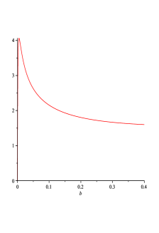
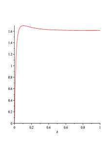
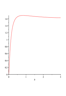
Figure 1. The graphs of $F(b,0.1)$, $F(b,0.25)$, and $F(b,0.5)$.

The unique point of maximum $b^{*}(\alpha)$ has the following asymptotic behaviour as $\alpha\to 0^{+}$. For a small $\alpha$ the main contribution in the sum in (5.1) comes from the term with $k=0$, that is, from

$$b^{5/3}\frac{1}{(\alpha^{3}+b)^{2}},$$

whose global maximum is attained at $b=5\alpha^{3}$ and equals $\frac{5^{5/3}}{36}\cdot\frac{1}{\alpha}$. Then (1.8) gives

$$\mathrm{K}_{2}(\alpha)\sim\frac{5^{13/3}}{3^{3/2}\,6^{4}\,\pi}\frac{1}{\alpha^{2}}=0.0505\frac{1}{\alpha^{2}}\ \text{as}\ \alpha\to 0,$$

while it follows from (1.7) that

$$\mathrm{K}_{1}(\alpha)\sim\frac{1}{4\pi^{2}}\frac{1}{\alpha^{2}}=0.025\frac{1}{\alpha^{2}}\ \text{as}\ \alpha\to 0,$$

which explains why $\mathrm{K}_{1}(\alpha)<\mathrm{K}_{2}(\alpha)$ near $\alpha=0$ and $\alpha=1$ in Fig. 2. On the other hand, in the middle region $|\frac{1}{2}-\alpha|\leq 0.2273$ the new estimate (1.8) is better. It is also worth pointing out that

$$\mathrm{K}_{2}(1/2)=\mathrm{K}_{2}(1/4)(=0.8819)$$

the equality holding since

$$F(b,1/2)=F(b/8,1/4).$$

The minimum with respect to $\alpha$ is attained at $\alpha^{*}=0.273$ giving $\mathrm{K}_{2}(\alpha^{*})=\mathrm{K}_{2}(1-\alpha^{*})=0.811$.

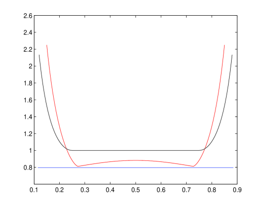
Figure 2. The graphs of $\mathrm{K}_{1}(\alpha)=\mathrm{k}(\alpha)^{2}$ (black) and $\mathrm{K}_{2}(\alpha)$ (red). The horizontal blue line is the constant in (5.2).

References

- [1] M. Aizenman and E.H. Lieb, On semi-classical bounds for eigenvalues of Schrödinger operators. Phys. Lett. 66A (1978), 427–429.
- [2] J. Dolbeault, A. Laptev, and M. Loss, Lieb–Thirring inequalities with improved constants. J. European Math. Soc. 10:4 (2008), 1121–1126.
- [3] J. Dolbeault, M.J. Esteban, A. Laptev, M. Loss, Interpolation inequalities and spectral estimates for magnetic operators, Ann. Henri Poincaré, 19 (2018), 1439–1463.
- [4] J. Dolbeault, M.J. Esteban, A. Laptev, M. Loss, Magnetic rings, J. Math. Phys., 59 (2018), 051504.
- [5] A. Eden and C. Foias, A simple proof of the generalized Lieb–Thirring inequalities in one space dimension. J. Math. Anal. Appl. 162 (1991), 250–254.
- [6] R.L. Frank, D. Hundertmark, M. Jex, P.T. Nam, The Lieb–Thirring inequality revisited. J. European Math. Soc. 23 (2021), 2583–2600.
- [7] R.L. Frank, A. Laptev, and T. Weidl, Schrödinger Operators: Eigenvalues and Lieb–Thirring Inequalities. (Cambridge Studies in Advanced Mathematics 200). Cambridge: Cambridge University Press, 2022.
- [8] A.Ilyin, A.Laptev, M.Loss, and S.Zelik, One-dimensional interpolation inequalities, Carlson-Landau inequalities, and magnetic Schrodinger operators. Int. Math. Res. Not. IMRN (2016) 2016:4, 1190–1222.
- [9] A.A. Ilyin and A.A. Laptev, Magnetic Lieb–Thirring inequality for periodic functions. Uspekhi Mat. Nauk 75:4 (2020), 207–208; English transl. in Russian Math. Surveys 75:4 (2020), 779–781.
- [10] A.A. Ilyin and A.A. Laptev, Lieb-Thirring inequalities on the torus. Mat. Sb. 207:10 (2016), 56–79; English transl. in Sb. Math. 207:9-10 (2016).
- [11] A. Ilyin, A. Laptev, and S. Zelik, Lieb–Thirring constant on the sphere and on the torus. J. Func. Anal. 279 (2020) 108784.
- [12] A. Laptev and T. Weidl, Sharp Lieb–Thirring inequalities in high dimensions. Acta Math. 184 (2000), 87–111.
- [13] A.I. Nazarov and A.P. Shcheglova, On the sharp constant in the “magnetic” 1D embedding theorem. Russ. J. Math. Phys. 25:1 (2018), 67–72.
- [14] S.V. Zelik and A.A.Ilyin, Green’s function asymptotics and sharp interpolation inequalities. Uspekhi Mat. Nauk 69:2 (2014), 23–76; English transl. in Russian Math. Surveys 69:2 (2014).