Constrained Causal Bayesian Optimization

Abstract

We propose constrained causal Bayesian optimization (ccbo), an approach for finding interventions in a known causal graph that optimize a target variable under some constraints. ccbo first reduces the search space by exploiting the graph structure and, if available, an observational dataset; and then solves the restricted optimization problem by modelling target and constraint quantities using Gaussian processes and by sequentially selecting interventions via a constrained expected improvement acquisition function. We propose different surrogate models that enable to integrate observational and interventional data while capturing correlation among effects with increasing levels of sophistication. We evaluate ccbo on artificial and real-world causal graphs showing successful trade off between fast convergence and percentage of feasible interventions.

B C E ØO Q U W V xx XX q y I ıi F

1 Introduction

The problem of understanding which interventions in a system optimize a target variable is of relevance in many scientific disciplines, including biology, medicine, and social sciences. Often, the investigator might want to solve this problem while also ensuring that interventions satisfy some constraints. As an example, consider the protein-signalling network of Fig. 1(a), which describes the causal pathways linking several phosphorylated proteins and phospholipids in human immune system cells, including the mitogen-activated protein kinases erk studied in cancer therapy (Frémin & Meloche, 2010; Sachs et al., 2005).

Figure 1: (a) Protein-signaling network and (b) causal psa graph. Red, grey and pink nodes indicate target, intervenable, and constrained variables respectively.

An investigator might wish to find which variables among $\text{{m}ek},\text{{pkc}},\text{{pka}}$ and akt to perturb and to which levels in order to minimize erk, under the constraints of not inhibiting pka and pkc which play an important role in the functioning of healthy cells. As another example, consider the graph of Fig. 1(b) describing the causal relationships between prostate specific antigen (psa) and its risk factors, some of which might be due to an existing policy at the time of study (Ferro et al., 2015). An investigator might wish to understand which variables among Aspirin, Statin, and Calories Intake (ci) to fix and to which values in order to minimize psa, under the constraint of keeping bmi below a certain value.

In this paper, we propose constrained causal Bayesian optimization (ccbo), a sequential approach for efficiently solving such constrained optimization problems in the setting of known causal graph that builds on the literature on causal Bayesian optimization (Aglietti et al., 2020), constrained Bayesian optimization (Gardner et al., 2014), and multi-task learning with Gaussian processes (gps) (Alvarez et al., 2011). Our contributions are summarized as follows:

• We provide a formalization of the constrained optimization problem using the framework of structural causal models (scms).
  

• We introduce a novel theory for reducing the search space of interventions that eliminates intervention sets of higher cardinality.
  

• We propose different gp surrogate models for the unknown target and constraint quantities that leverage observational data, interventional data and the scm structure, capturing correlations with increasing level of sophistication. This enables uncertainty quantification thereby speeding up the identification of an optimal intervention while limiting the number of infeasible interventions, i.e. not satisfy the constraints.
  

• We propose a constrained expected improvement acquisition function for sequentially selecting interventions based on both output optimization and constraint satisfaction. This enables finding the optimal solution with a smaller number of interventions.
  

• We evaluate ccbo on synthetic and real-world graphs with different scm characteristics showing how it successfully trades off achieving a fast convergence and collecting a high percentage of feasible interventions.

2 Constrained Causal Global Optimization

We consider a system of observable random variables $\V$ with target variable $Y\in\V$ and intervenable variables $\I\subseteq\V\backslash Y$, and the problem of finding an intervention set $\mathbf{X}^{*}\subseteq\I$ and intervention values $\mathbf{x}^{*}$ that optimize the expectation of $Y$ while ensuring that the expectations of constrained variables $\C\subseteq\V\backslash Y$ are above/below certain values.

We assume that the system can be described by a structural causal model (scm) (Pearl, 2000; Pearl et al., 2016) ${\cal M}=\langle\V,\U,\F,p(\U)\rangle$, where $\U$ is a set of exogenous unobserved random variables with distribution $p(\U)=\prod_{U\in\U}p(U)$, and $\F=\{f_{V}\}_{V\in\V}$ is a set of deterministic functions such that $V=f_{V}(\text{pa}(V),\U_{V})$ with $\text{pa}(V)\subseteq\V\backslash V$ and $\U_{V}\subseteq\U$, $\forall V\in\V$. ${\cal M}$ has associated a causal graph $\mathcal{G}$ with nodes $\V$, and with a directed edge from $V$ to $W$ if $V\in\text{pa}(W)$, in which case $V$ is called a parent of $W$, and a bi-directed edge between $V$ and $W$ if $\U_{V}\cap\U_{W}\neq\emptyset$ ($\U_{V}\cap\U_{W}$ is an unobserved confounder between $V$ and $W$). We assume that $\mathcal{G}$ is acyclic, namely that there are no directed paths starting and ending at the same node. We refer to the joint distribution of $\V$ determined by $p(\U)$, which we denote by $p(\V)$, as observational distribution, and to an observation from $p(\V)$ as observational data sample.

An intervention on $V\in\I$ setting its value to $v$, denoted by $\text{do}(V=v)$, corresponds to modifying ${\cal M}$ by replacing $f_{V}(\text{pa}(V),\U_{V})$ with $v$. We refer to the joint distribution of $\V$ in the modified scm under such an intervention, indicated by $p_{\text{do}(V=v)}(\V)$, as interventional distribution, and to an observation from it as interventional data sample. Notice that, in the case of no unobserved confounders, $p_{\text{do}(V=v)}(\V)=\prod_{W\in\V\backslash V}p(W\,|\,\text{pa}(W))\delta_{V=v}$ with $\delta_{V=v}$ denoting a delta function centered at $v$. An intervention on a set of variables is defined similarly.

Let $\mu_{\text{do}(\mathbf{X}=\mathbf{x})}^{Y}:=\mathbb{E}_{p_{\text{do}(\mathbf{X}=\mathbf{x})}}[Y]$ denote the expectation of $Y$ w.r.t. the interventional distribution, which we refer to as the target effect. The goal of the investigator is to find a set $\mathbf{X}^{*}\subseteq\I$ and values $\mathbf{x}^{*}$ that optimize the target effect while ensuring that $\mu_{\text{do}(\mathbf{X}^{*}=\mathbf{x}^{*})}^{C}$, which we refer to as constraint effect, is greater/smaller than a threshold $\lambda^{C}$, $\forall C\in\C\subseteq\V\backslash Y$. Target and constraint effects are unknown.

The constraint for a variable $X\in\C\cap\mathbf{X}$ can directly be enforced by restricting the range of intervention values, $D(X)$, to be in accordance with the threshold. Instead, the constraints for $\C_{\mathbf{X}}:=\C\backslash(\C\cap\mathbf{X})$ need to be included in the optimization problem. The constrained optimization problem can thus be formalized as follows.

Definition 2.1 (ccgo Problem).

The constrained causal global optimization (ccgo) problem is the problem of finding a tuple $(\mathbf{X}^{*},\mathbf{x}^{*})$ such that

$$\mathbf{X}^{*},\mathbf{x}^{*} =\operatorname*{arg\,min}_{\begin{subarray}{c}\mathbf{X}\in\mathcal{P}_{\I},\\ \mathbf{x}\in D(\mathbf{X})\end{subarray}}\mu_{\text{do}(\mathbf{X}=\mathbf{x})}^{Y}\,\,\textrm{ s.t. }\mu_{\text{do}(\mathbf{X}=\mathbf{x})}^{\C_{\mathbf{X}}}\geq\lambda^{\C_{\mathbf{X}}},$$ (1)

where $\mathcal{P}_{\I}$ indicates the power set of $\I$, $D(\mathbf{X}):=\times_{X\in\mathbf{X}}D(X)$, and $\mu_{\text{do}(\mathbf{X}=\mathbf{x})}^{\C_{\mathbf{X}}}$ and $\lambda^{\C_{\mathbf{X}}}$ denote the constraint effects and corresponding thresholds on all variables in $\C_{\mathbf{X}}$.

The ccgo problem extends the causal global optimization (cgo) problem defined in Aglietti et al. (2020) to incorporate constraints.

3 Constrained Causal Bayesian Optimization

Inputs: $\mathcal{G}$, $\I,\C,Y$, $\mathcal{D}^{I}:=\{\mathcal{D}^{I}_{\mathbf{X}}\}_{\mathbf{X}\subseteq\I}$, $\mathcal{D}^{O}$, $\lambda^{\C}$, $S$, $T$

$n\mathbb{M}_{\C\cup Y,\mathcal{G}}\leftarrow\texttt{cMISReduce}(\mathcal{G},\I,\C,Y,\mathcal{D}^{O})$

Initialise gps  $g_{\mathbf{X}}(\mathbf{x})$ $\forall\mathbf{X}\in n\mathbb{M}_{\C\cup Y,\mathcal{G}}$ with $\mathcal{D}^{I}_{\mathbf{X}}$ and $\mathcal{D}^{O}$

for $t=1,\ldots,T$ do

       1. Select intervention $(\mathbf{X}_{t},\mathbf{x}_{t})$ with cei

       2. Obtain $S$ samples $\{\mathbf{c}_{\mathbf{X}_{t}}^{(s)},y^{(s)}\}_{s=1}^{S}$ from the distribution $p_{\text{do}(\mathbf{X}_{t}=\mathbf{x}_{t})}(\C_{\mathbf{X}_{t}},Y)$, and use them to compute the sample mean estimate $\hat{\mu}_{\text{do}(\mathbf{X}_{t}=\mathbf{x}_{t})}$

       3. Update dataset $\mathcal{D}^{I}_{\mathbf{X}_{t}}\leftarrow\mathcal{D}^{I}_{\mathbf{X}_{t}}\cup(\mathbf{x}_{t},\hat{\mu}_{\text{do}(\mathbf{X}_{t}=\mathbf{x}_{t})})$

       4. Update gps for $g_{\mathbf{X}_{t}}(\mathbf{x})\,|\,\mathcal{D}^{I}_{\mathbf{X}_{t}}$

end for

Output: $(\mathbf{X}^{\star},\mathbf{x}^{\star})$ with min feasible $\hat{\mu}^{Y}_{\text{do}(\mathbf{X}^{\star}=\mathbf{x}^{\star})}$ over $\mathcal{D}^{I}$

Algorithm 1 ccbo

We propose to solve the ccgo problem using the constrained causal Bayesian optimization (ccbo) method summarized in Algorithm 1, which assumes known casual graph $\mathcal{G}$, continuous variables $\V$, and full observation of the system after an intervention. First, the search space is reduced to a subset $n\mathbb{M}_{\C\cup Y,\mathcal{G}}$ of $\mathcal{P}_{\I}$ via the cMISReduce procedure described in Section 3.1. Then, the restricted ccgo problem is solved by modelling, $\forall\mathbf{X}\in n\mathbb{M}_{\C\cup Y,\mathcal{G}}$, the unknown target and constraint effects $\mu_{\text{do}(\mathbf{X}=\mathbf{x})}:=(\mu_{\text{do}(\mathbf{X}=\mathbf{x})}^{Y},\mu_{\text{do}(\mathbf{X}=\mathbf{x})}^{\C_{\mathbf{X}}})$ using Gaussian processes (gps) (Rasmussen & Williams, 2006) $g_{\mathbf{X}}(\mathbf{x}):=\big{(}g^{V}_{\mathbf{X}}(\mathbf{x})\big{)}_{V\in\C_{\mathbf{X}}\cup Y}$, as described in Section 3.2, and via the following sequential strategy. At each trial $t=1,\ldots,T$: (1) a set of intervenable variables $\mathbf{X}_{t}$ and intervention values $\mathbf{x}_{t}$ are selected via a constrained expected improvement (cei) acquisition function that accounts for both the target and constraint effects, as described in Section 3.3; (2) a set of $S$ interventional data samples is obtained and used to get a sample mean estimate $\hat{\mu}_{\text{do}(\mathbf{X}_{t}=\mathbf{x}_{t})}$ of $\mu_{\text{do}(\mathbf{X}_{t}=\mathbf{x}_{t})}$; (3) $(\mathbf{x}_{t},\hat{\mu}_{\text{do}(\mathbf{X}_{t}=\mathbf{x}_{t})})$ is added to the interventional dataset $\mathcal{D}^{I}_{\mathbf{X}_{t}}$ of $\mathbf{X}_{t}$; (4) the gps for $g_{\mathbf{X}_{t}}(\mathbf{x})$ are updated using $\mathcal{D}^{I}_{\mathbf{X}_{t}}$. Once the maximum number of trials $T$ is reached, a tuple $(\mathbf{X}^{\star},\mathbf{x}^{\star})$ giving the minimum feasible target effect value in $\mathcal{D}^{I}:=\{\mathcal{D}^{I}_{\mathbf{X}}\}_{\mathbf{X}\subseteq\I}$ is returned.

3.1 Reducing the Search Space

The cardinality of the power set, $|\mathcal{P}_{\I}|$, grows exponentially with the cardinality of $\I$, thus solving the ccgo problem by exploring the entire set could be prohibitively expensive. Even when $|\mathcal{P}_{\I}|$ is small, reducing the search space would simplify the problem as a smaller number of comparisons between constraint and target effects would be required. In this section, we propose a procedure, which we refer to as cMISReduce, that leverages invariances of the target and constraint effects w.r.t. different intervention sets to eliminate intervention sets of higher cardinality. This is achieved by extending the theory of minimal intervention sets of Lee & Bareinboim (2018) to account for the presence of constraints (a summary of the procedure and all proofs are given Appendix A).

The search space is first reduced from $\mathcal{P}_{\I}$ to the set of constrained minimal intervention sets (cmiss) relative to $({\C\cup Y},\mathcal{G})$, denoted by $\mathbb{M}_{\C\cup Y,\mathcal{G}}$.

Definition 3.1 (cmis).

A set $\mathbf{X}\subseteq\I$ is said to be a cmis relative to $(\C\cup Y,\mathcal{G})$ if there is no $\mathbf{X}^{\prime}\subset\mathbf{X}$ with $\C_{\mathbf{X}}=\C_{\mathbf{X}^{\prime}}$ such that $\mu_{\text{do}(\mathbf{X}=\mathbf{x})}^{W}=\mu_{\text{do}(\mathbf{X}^{\prime}=\mathbf{x}^{\prime})}^{W}$, where $\mathbf{x}^{\prime}$ indicates the subset of $\mathbf{x}$ corresponding to variables $\mathbf{X}^{\prime}$, $\forall\mathbf{x}\in D(\mathbf{X})$, $\forall W\in\C_{\mathbf{X}}\cup Y$, and $\forall$ scm with causal graph $\mathcal{G}$.

The following theorem justifies this reduction.

Theorem 3.2 (Sufficiency of $\mathbb{M}_{\C\cup Y,\mathcal{G}}$).

$\mathbb{M}_{\C\cup Y,\mathcal{G}}$ contains a solution of the ccgo problem (if a solution exists), $\forall$ scm with causal graph $\mathcal{G}$.

Let $\text{an}(W,\mathcal{G})$ be the set of ancestors of $W$ in $\mathcal{G}$, i.e. the nodes with a directed path to $W$; $\text{an}(\W,\mathcal{G}):=\cup_{W\in\W}\text{an}(W,\mathcal{G})$; and $\mathcal{G}_{\overline{\mathbf{X}}}$ the graph with all incoming links onto all elements of $\mathbf{X}$ removed. The following proposition gives a graphical criterion for identifying $\mathbb{M}_{\C\cup Y,\mathcal{G}}$.

Proposition 3.3 (Characterization of cmis).

$\mathbf{X}\subseteq\I$ is a cmis relative to $({\C\cup Y},\mathcal{G})$ $\iff$ $\mathbf{X}\subseteq\text{an}(\C\cup Y,\mathcal{G}_{\overline{\mathbf{X}}})\cup(\C\cap\mathbf{X})$.

If an observational dataset $\mathcal{D}^{O}$ is available, the search space is further reduced from $\mathbb{M}_{\C\cup Y,\mathcal{G}}$ to $n\mathbb{M}_{\C\cup Y,\mathcal{G}}$ by checking, $\forall\mathbf{X}\in\mathbb{M}_{\C\cup Y,\mathcal{G}}$, if all reducible variables in $\C_{\mathbf{X}}$ are null-feasible.

Definition 3.4 (Reducibility).

$C\in\C_{\mathbf{X}}$ is reducible if $\mu_{\text{do}(\mathbf{X}=\mathbf{x})}^{C}=\mu^{C}:=\mathbb{E}_{p}[C]$, $\forall\mathbf{x}\in D(\mathbf{X})$.

Definition 3.5 (Null-feasibility).

$C\in\C_{\mathbf{X}}$ is null-feasible if $\mu^{C}\geq\lambda^{C}$.

If $\mathbf{X}\cap\text{an}(C,\mathcal{G}_{\overline{\mathbf{X}}})=\emptyset$, $C\in\C_{X}$ is reducible. Indeed, if $\mathbf{X}\cap\text{an}(C,\mathcal{G}_{\overline{\mathbf{X}}})=\emptyset$, by Lemma A.1 in Appendix A (with $\W_{1}=\mathbf{X},\W_{2}=C,\W_{3}=\emptyset$) we have $C\rotatebox[origin={c}]{90.0}{$\models$}_{\mathcal{G}_{\overline{\mathbf{X}}}}\mathbf{X}$, which implies $\mu_{\text{do}(\mathbf{X}=\mathbf{x})}^{C}=\mu^{C}$ by rule 3 of do-calculus (Pearl, 2000).

If a reducible $C\in\C_{X}$ is not null-feasible, $\mathbf{X}$ is removed from the search space as it is not a solution of the ccgo problem. If instead $C$ is null-feasible, all $\mathbf{X}^{\prime}\supset\mathbf{X}$ in $\mathbb{M}_{\C\cup Y,\mathcal{G}}$ that are of the form $\mathbf{X}^{\prime}=\mathbf{X}\cup\mathbf{X}_{1}$ where $\mathbf{X}_{1}\cap\text{an}(\C_{\mathbf{X}}\backslash C\cup Y,\mathcal{G}_{\overline{\mathbf{X}^{\prime}}})=\emptyset$, and for which (i) $\C_{\mathbf{X}^{\prime}}=\C_{\mathbf{X}}$ or (ii) all variables in $\C_{\mathbf{X}}\backslash\C_{\mathbf{X}^{\prime}}$ are reducible and null-feasible, are eliminated from the search space. Indeed, in such cases, if $\mathbf{X}^{\prime}$ were a solution of the ccgo problem, then $\mathbf{X}$ would also be a solution as: (a) $\forall W\in(\C_{\mathbf{X}}\backslash C)\backslash(\C\cap\mathbf{X}_{1})\cup Y$, $\mu_{\text{do}(\mathbf{X}^{\prime}=\mathbf{x}^{\prime})}^{W}=\mu_{\text{do}(\mathbf{X}=\mathbf{x})}^{W}$ (Lemma A.1 in Appendix A (with $\W_{1}=\mathbf{X}_{1},\W_{2}=\C_{\mathbf{X}}\backslash C\cup Y,\W_{3}=\mathbf{X}$) gives $\C_{\mathbf{X}}\backslash C\cup Y\rotatebox[origin={c}]{90.0}{$\models$}_{\mathcal{G}_{\overline{\mathbf{X}^{\prime}}}}\mathbf{X}_{1}\,|\,\mathbf{X}$, which implies $\mu_{\text{do}(\mathbf{X}^{\prime}=\mathbf{x}^{\prime})}^{W}=\mu_{\text{do}(\mathbf{X}=\mathbf{x})}^{W}$ by rule 3 of do-calculus); (b) $\forall W\in\C\cap\mathbf{X}_{1}$ the constraint effects are satisfied for $\mathbf{X}$ as $\C\cap\mathbf{X}_{1}=\C_{\mathbf{X}}\backslash\C_{\mathbf{X}^{\prime}}$.

Figure 2: (a) Causal graph with $\I=\{A,D,E\}$ and $\C=\{C,D,E\}$. (b) Causal graph with $\I=\C=\{X,Z\}$.

Example: We describe the search space reduction for the casual graph of Fig. 2(a). In this graph $\mathbb{M}_{\C\cup Y,\mathcal{G}}=\mathcal{P}_{\I}=\{\{A\},\{D\},\{E\},\{A,D\},\{A,E\},\{D,E\},\{A,D,E\}\}$, as $\mathbf{X}\subseteq\text{an}(\C\cup Y,\mathcal{G}_{\overline{\mathbf{X}}})\cup(\C\cap\mathbf{X})$, $\forall\mathbf{X}\in\mathcal{P}_{\I}$ (e.g. $A\in\text{an}\big{(}\C\cup Y,\mathcal{G}_{\overline{A}}\big{)}\cup(\C\cap A)$). Consider $\mathbf{X}=\{D,E\}\in\mathbb{M}_{\C\cup Y,\mathcal{G}}$ and $C$. $\mathbf{X}\cap\text{an}\left(C,\mathcal{G}_{\overline{\mathbf{X}}}\right)=\emptyset$, and therefore $C$ is reducible. If $C$ is not null-feasible, $\mathbf{X}$ is removed from the search space. If instead $C$ is null-feasible, the set $\mathbf{X}^{\prime}=\{A,D,E\}\supset\mathbf{X}$ in $\mathbb{M}_{\C\cup Y,\mathcal{G}}$ is of the form $\mathbf{X}^{\prime}=\mathbf{X}\cup A$ where $A\not\in\text{an}(\C_{\mathbf{X}}\backslash C\cup Y,\mathcal{G}_{\overline{\mathbf{X}^{\prime}}})$. Therefore $\mathbf{X}^{\prime}$ is removed from the search space. All other sets in $\mathbb{M}_{\C\cup Y,\mathcal{G}}$ have constrained variables that are non reducible and thus need to be included in $n\mathbb{M}_{\C\cup Y,\mathcal{G}}$.

3.2 Gaussian Processes Surrogate Models

For each $\mathbf{X}\in n\mathbb{M}_{\C\cup Y,\mathcal{G}}$ and $V\in\C_{\mathbf{X}}\cup Y$, we model $\mu^{V}_{\text{do}(\mathbf{X}=\mathbf{x})}$ with a gp $g^{V}_{\mathbf{X}}(\mathbf{x})\sim\mathcal{GP}(m^{V}_{\mathbf{X}}(\mathbf{x}),S^{V}_{\mathbf{X}}(\mathbf{x},\mathbf{x}^{\prime}))$, as gps allow constructing flexible surrogate models while enabling uncertainty quantification and closed form updates. We propose one single-task gp (stgp) and two multi-task gps (mtgp and $\mathcal{G}$-mtgp) which capture the correlation across effects with increasing level of sophistication.

For $V\neq W$, the single-task gp treats $g^{V}_{\mathbf{X}}(\mathbf{x})$ and $g^{W}_{\mathbf{X}}(\mathbf{x}^{\prime})$ as independent, while the multi-task gps model their correlation via a covariance matrix $S^{V,W}_{\mathbf{X}}(\mathbf{x}_{1},\mathbf{x}_{2})$, with $(i,j)$-th element given by $\mathbb{E}[g^{V}_{\mathbf{X}}(\mathbf{x}_{i})g^{W}_{\mathbf{X}}(\mathbf{x}_{j})]-\mathbb{E}[g^{V}_{\mathbf{X}}(\mathbf{x}_{i})]\mathbb{E}[g^{W}_{\mathbf{X}}(\mathbf{x}_{j})]$, either by assuming a common latent structure among the gps (mtgp) or, for the setting of no unobserved confounders and under the assumption $V=f_{V}(\text{pa}(V))+U_{V}$ with $p(U_{V})={\cal N}(0,\sigma^{2}_{V})$, by explicitly exploiting the scm structure ($\mathcal{G}$-mtgp). We propose different prior parameters constructions for stgp and mtgp, including one that leverages the availability of an observational dataset $\mathcal{D}^{O}$ (stgp⁺ and mtgp⁺). The different gp constructions allow the investigator to model the target and constraint effects in both settings where no information about the system is available and black-box models are preferred (stgp and mtgp) and settings in which one can leverage different sources of information and integrate them in a structured prior formulation that quantifies uncertainty in a principled way (stgp⁺, mtgp⁺, and $\mathcal{G}$-mtgp).

For all surrogate models, after an intervention $(\mathbf{X},\mathbf{x})$ is selected by the acquisition function, as described in Section 3.3, a set of $S$ interventional data samples $\{\mathbf{c}^{(s)}_{\mathbf{X}},y^{(s)}\}_{s=1}^{S}$ from $p_{\text{do}(\mathbf{X}=\mathbf{x})}(\C_{\mathbf{X}},Y)$ is obtained. For each $V\in\C_{\mathbf{X}}\cup Y$, this set is used to form a sample mean estimate $\hat{\mu}_{\text{do}(\mathbf{X}=\mathbf{x})}^{V}$ of $\mu_{\text{do}(\mathbf{X}=\mathbf{x})}^{V}$, which is treated as a noisy realization of $g^{V}_{\mathbf{X}}(\mathbf{x})$ with additive Gaussian noise. The tuple $(\mathbf{x},\hat{\mu}_{\text{do}(\mathbf{X}=\mathbf{x})})$ is then added to $\mathcal{D}^{I}_{\mathbf{X}}$ and the posterior distribution of $g_{\mathbf{X}}(\mathbf{x})$, denoted by $\tau(g_{\mathbf{X}}\,|\,\mathcal{D}^{I}_{\mathbf{X}})$, is computed via standard gp updates (Rasmussen & Williams, 2006). Full details are given in Appendix B.

stgp. For the single-task gp, we either assume $m^{V}_{\mathbf{X}}(\mathbf{x})=0$ and radial basis function (rbf) kernel $S^{V}_{\mathbf{X}}(\mathbf{x},\mathbf{x}^{\prime})=\sigma^{2}_{f}\exp(-\frac{||\mathbf{x}-\mathbf{x}^{\prime}||^{2}}{2l^{2}})$ with $(\sigma^{2}_{f},l)$ hyper-parameters, or the prior construction proposed in cbo (Aglietti et al., 2020). In the latter case, $\mathcal{D}^{O}$ is used to obtain estimates of the target and constraint effects which are then used as prior mean functions (we refer to this variant as stgp⁺).

mtgp. Our first multi-task gp, inspired by the linear coregionalization model of Alvarez et al. (2011), assumes that the target and constraint gps are linear combinations of shared independent gps, i.e. $g^{V}_{\mathbf{X}}(\mathbf{x})=\sum_{q=1}^{Q}a^{V}_{\mathbf{X},q}u_{\mathbf{X},q}(\mathbf{x})$ with $u_{\mathbf{X},q}(\mathbf{x})\sim\mathcal{GP}(m_{\mathbf{X},q}(\mathbf{x}),S_{\mathbf{X},q}(\mathbf{x},\mathbf{x}^{\prime}))$. In this case, the variance and covariance terms across functions and intervention values are given by $S^{V}_{\mathbf{X}}(\mathbf{x},\mathbf{x}^{\prime})=\sum_{q=1}^{Q}\left(a^{V}_{\mathbf{X},q}\right)^{2}S_{\mathbf{X},q}(\mathbf{x},\mathbf{x}^{\prime})$ and $S^{V,W}_{\mathbf{X}}(\mathbf{x},\mathbf{x}^{\prime})=\sum_{q=1}^{Q}a^{V}_{\mathbf{X},q}a^{W}_{\mathbf{X},q}S_{\mathbf{X},q}(\mathbf{x},\mathbf{x}^{\prime})$ respectively. The scalar parameters $a^{V}_{\mathbf{X},q}$ are learned with a standard type-2 ml approach together with the kernel hyper-parameters. We either consider $m_{\mathbf{X},q}(\mathbf{x})=0$ and rbf kernel for each $S_{\mathbf{X},q}(\mathbf{x},\mathbf{x}^{\prime})$, or the prior construction using $\mathcal{D}^{O}$ as in stgp⁺ (we refer to this variant as mtgp⁺).

$\mathcal{G}$-mtgp. For the setting of no unobserved confounders and under the assumption $V=f_{V}(\text{pa}(V))+U_{V}$ with $p(U_{V})={\cal N}(0,\sigma^{2}_{V})$, we propose to model each $f_{V}$ as an independent gp with an rbf kernel $f_{V}(\text{pa}(v))\sim\mathcal{GP}(0,S^{V}_{\textsc{rbf}}(\text{pa}(v),\text{pa}(v)^{\prime}))$, where $\text{pa}(v)$ denotes a value taken by $\text{pa}(V)$, and to fit it using $\mathcal{D}^{O}$. Consider the intervention $\text{do}(\mathbf{X}=\mathbf{x})$ and let $\U^{\text{an}(V)}_{\mathbf{X}}$ denote the subset of $\U$ corresponding to the ancestors of $V$ in $\mathcal{G}$ that are not d-separated from $V$ by $\mathbf{X}$, and similarly for $f^{\text{an}(V)}_{\mathbf{X}}$. We can write $V$ as an explicit function of $\U^{\text{an}(V)}_{\mathbf{X}}$ and $f^{\text{an}(V)}_{\mathbf{X}}$ by recursively replacing parents with their functional form in the modified scm under $\text{do}(\mathbf{X}=\mathbf{x})$. Taking the expectation w.r.t. $\U^{\text{an}(V)}_{\mathbf{X}}$ therefore gives $g^{V}_{\mathbf{X}}(\mathbf{x})$ as a function of $f^{\text{an}(V)}_{\mathbf{X}}$.

For example, for the causal graph in Fig. 2(b) with $X=U_{X}$, $Z=f_{Z}(X)+U_{Z}$ and $Y=f_{Y}(Z)+U_{Y}$, we can write $Y=f_{Y}(f_{Z}(X)+U_{Z})+U_{Y}$, which gives $g^{Y}_{X}(x)=\mathbb{E}_{p(U_{Z})}[f_{Y}(f_{Z}(x)+U_{Z})]$ and $g^{Z}_{X}(x)=f_{Z}(x)$. We can then obtain realizations $\{g^{V,(s)}_{\mathbf{X}}\}_{s=1}^{S^{\prime}}$ of $g^{V}_{\mathbf{X}}$ by using samples of $f^{\text{an}(V)}_{\mathbf{X}}$ and $\U^{\text{an}(V)}_{\mathbf{X}}$ to form an approximation of $S^{V,W}_{\mathbf{X}}(\mathbf{x}_{1},\mathbf{x}_{2})$ as $\frac{1}{S^{\prime}}\sum_{s=1}^{S^{\prime}}g^{V,(s)}_{\mathbf{X}}(\mathbf{x}_{1})g^{W,(s)}_{\mathbf{X}}(\mathbf{x}_{2})-\Big{(}\frac{1}{S^{\prime}}\sum_{s=1}^{S^{\prime}}g^{V,(s)}_{\mathbf{X}}(\mathbf{x}_{1})\Big{)}\Big{(}\frac{1}{S^{\prime}}\sum_{s=1}^{S^{\prime}}g^{W,(s)}_{\mathbf{X}}(\mathbf{x}_{2})\Big{)}$, and similarly for $S^{V}_{\mathbf{X}}(\mathbf{x},\mathbf{x}^{\prime})$ and $m_{\mathbf{X}}^{V}(\mathbf{x})$.

3.3 Acquisition Functions

To select interventions accounting for both the target and constraint effects we propose acquisition functions based on those used for constrained bo (Gardner et al., 2014) and noisy bo (Letham et al., 2019). We define the constrained expected improvement (cei) per unit of intervention cost at an input point $\mathbf{x}$ as $c\textsc{ei}_{\mathbf{X}}(\mathbf{x}):=\mathbb{E}_{\tau(g_{\mathbf{X}}\,|\,\mathcal{D}^{I}_{\mathbf{X}})}\left[\frac{\max(0,g^{Y}-g^{Y}_{\mathbf{X}}(\mathbf{x}))}{|\mathbf{X}|}\mathbb{I}_{g^{\C_{\mathbf{X}}}_{\mathbf{X}}\geq\lambda^{\C_{\mathbf{X}}}}\right]$, where $g^{Y}$ is the minimum feasible value attained by $g^{Y}_{\mathbf{X}}$ across interventional dataset $\mathcal{D}^{I}$ and $\mathbb{I}_{g^{\C_{\mathbf{X}}}_{\mathbf{X}}\geq\lambda^{\C_{\mathbf{X}}}}$ is an indicator variable equal to one if $g^{\C_{\mathbf{X}}}_{\mathbf{X}}\geq\lambda^{\C_{\mathbf{X}}}$ and to zero otherwise. The division by $|\mathbf{X}|$ is due to assuming an intervention cost for $\mathbf{X}$ equal to its cardinality. Alternative costs can be considered as long as they are greater than zero.

stgp. When using a single-task gp as surrogate model, we can exploit the factorization $\tau(g_{\mathbf{X}}\,|\,\mathcal{D}^{I}_{\mathbf{X}})=\tau(g^{Y}_{\mathbf{X}}\,|\,\mathcal{D}^{I}_{\mathbf{X}})\prod_{C\in\C_{\mathbf{X}}}\tau(g^{C}_{\mathbf{X}}\,|\,\mathcal{D}^{I}_{\mathbf{X}})$ to obtain $c\textsc{ei}_{\mathbf{X}}(\mathbf{x})=\mathbb{E}_{\tau(g^{Y}_{\mathbf{X}}\,|\,\mathcal{D}^{I}_{\mathbf{X}})}\left[\max(0,g^{Y}-g^{Y}_{\mathbf{X}}(\mathbf{x}))\right]\prod_{C\in\C_{\mathbf{X}}}\mathbb{P}(g^{C}_{\mathbf{X}}\geq\lambda_{C})$ where $\mathbb{P}(g^{C}_{\mathbf{X}}\geq\lambda_{C})=\Big{[}1-\Phi\left(\frac{\lambda_{C}-m_{\mathbf{X}}^{C}(\mathbf{x})}{S_{\mathbf{X}}^{C}(\mathbf{x},\mathbf{x})}\right)\Big{]}$ with $\Phi(\cdot)$ denoting the cdf of a standard Gaussian random variable. In the case of noiseless observations of $g^{V_{k}}_{\mathbf{X}}(\mathbf{x})$, $g^{Y}$ is known thus we can compute the first term in closed form as $\left(g^{Y}-m^{Y}_{\mathbf{X}}(\mathbf{x})\right)\Phi\left(\frac{g^{Y}-m^{Y}_{\mathbf{X}}(\mathbf{x})}{S^{Y}_{\mathbf{X}}(\mathbf{x},\mathbf{x})}\right)+S^{Y}_{\mathbf{X}}(\mathbf{x},\mathbf{x})\phi\left(\frac{g^{Y}-m^{Y}_{\mathbf{X}}(\mathbf{x})}{S^{Y}_{\mathbf{X}}(\mathbf{x},\mathbf{x})}\right)$ with $\phi(\cdot)$ denoting the pdf of a standard Gaussian random variable. In the case of noisy observations of $g^{V_{k}}_{\mathbf{X}}(\mathbf{x})$, $g^{Y}$ is unknown as we observe noisy values of the target effects. We can get an estimate of $g^{Y}$ using samples from $\tau(g_{\mathbf{X}}\,|\,\mathcal{D}^{I}_{\mathbf{X}})$ for all $\mathbf{X}\in n\mathbb{M}_{\C\cup Y,\mathcal{G}}$, and use the estimate to compute $c\textsc{ei}_{\mathbf{X}}(\mathbf{x})$ in closed form using the terms derived above. For every $\mathbf{X}\in n\mathbb{M}_{\C\cup Y,\mathcal{G}}$ the values of $c\textsc{ei}_{\mathbf{X}}(\mathbf{x})$ obtained with different $g^{Y}$ are then averaged to integrate out the uncertainty on the optimal feasible value observed across all intervention sets.

mtgp. When using a multi-task model, $c\textsc{ei}_{\mathbf{X}}(\mathbf{x})$ cannot be computed in closed form as $\tau(g_{\mathbf{X}}\,|\,\mathcal{D}^{I}_{\mathbf{X}})$ does not factorize. We thus compute it via Monte Carlo integration with a similar procedure as for the noisy stgp setting.

3.4 Computational Aspects

The computational cost of ccbo is dominated by the algebraic operations needed to compute the posterior parameters for the gp models of the target and constraints effects. Let $N_{I}$ denote the largest among the cardinalities of the interventional datasets collected for the sets in $n\mathbb{M}_{\C\cup Y,\mathcal{G}}$, i.e. $N_{I}=\max_{\mathbf{X}\in n\mathbb{M}_{\C\cup Y,\mathcal{G}}}{|\mathcal{D}^{I}_{\mathbf{X}}|}$, and let $M$ denote the highest among the number of target and constraint effects for the sets in $n\mathbb{M}_{\C\cup Y,\mathcal{G}}$, i.e. $M=\max_{\mathbf{X}\in n\mathbb{M}_{\C\cup Y,\mathcal{G}}}{1+|C_{\mathbf{X}}|}$. As the gps corresponding to different intervention sets are updated independently, the computational cost scales as $O(N_{I}^{3})$ when using a single-task model and as $O(M^{3}N_{I}^{3})$ when using a multi-task model. Independent gps updates also imply linear scaling of the computational complexity with respect to the cardinality of $n\mathbb{M}_{\C\cup Y,\mathcal{G}}$. Therefore, a larger $\mathcal{G}$ might induce a higher number of sets to explore, but does not induce higher computational complexity.

In terms of convergence to the true global optimum, ccbo inherits the properties of bo algorithms. While any alternative acquisition function for constrained bo can be used within ccbo, in this work we resort to a constrained expected improvement function due to its computationally tractability. The expected improvement acquisition function was shown to have strong theoretical guarantees (Vazquez & Bect, 2010; Bull, 2011) while performing well in practice (Snoek et al., 2012). However, performance guarantees have yet to be established for the constrained version.

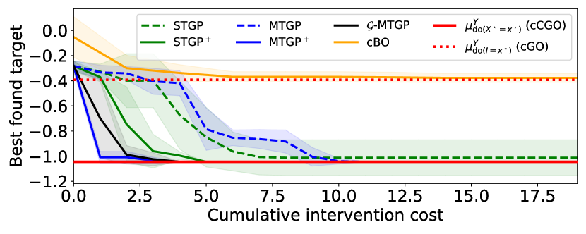
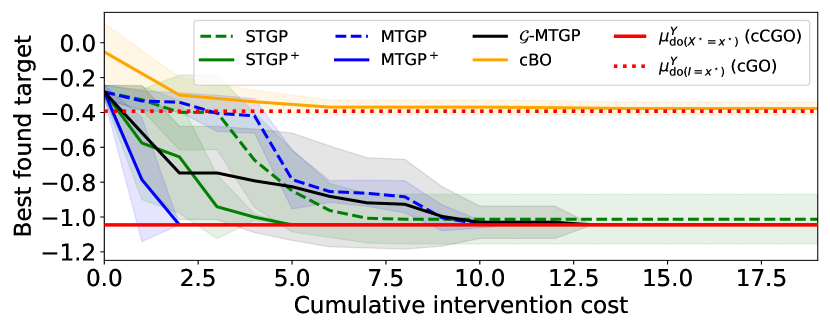
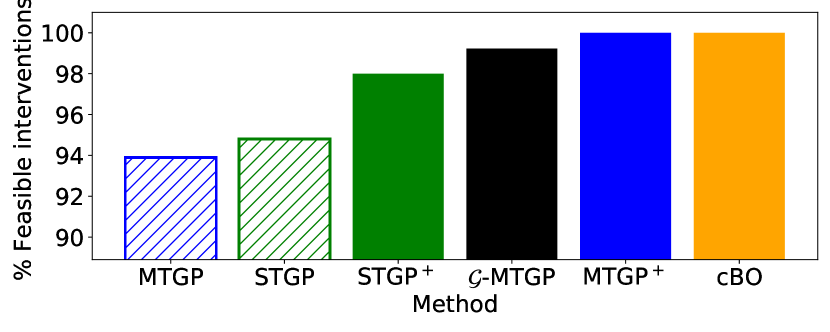
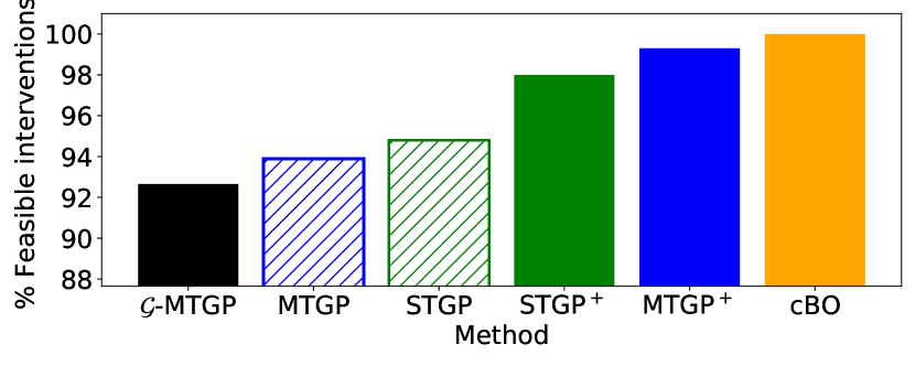
Figure 3: synthetic-1 with $N_{O}=500$ (top row) and $N_{O}=100$ (bottom row) and $\lambda^{Z}=2$. Left: Causal graphs. Center: Convergence to the ccgo (solid red line) and cgo (dotted red line) optima. Lines give average results across different initialization of $\mathcal{D}^{I}$. Shaded areas represent $\pm$ standard deviation. Right: Average percentage of feasible interventions collected over trials.

3.5 Related Work

ccbo is related to the vast literature on constrained bo methods, which find feasible solutions either by using an acquisition function that accounts for the probability of feasibility (Gardner et al., 2014; Gelbart et al., 2014; Griffiths & Hernández-Lobato, 2017; Hernández-Lobato et al., 2014; Keane et al., 2008; Schonlau et al., 1998; Sóbester et al., 2014; Tran et al., 2019), or by transforming the constrained problem into an unconstrained one (Ariafar et al., 2019; Picheny et al., 2016), or by exploiting trust regions (Eriksson & Poloczek, 2021). While these works disregard the causal aspect of the optimization and model the unknown functions independently, multi-task surrogate models have been considered by multi-objective bo methods (Dai et al., 2020; Feliot et al., 2017; Hakhamaneshi et al., 2021; Mathern et al., 2021; Swersky et al., 2013) or, more recenlty, in the context of safe bo (Bergmann & Graichen, 2020; Berkenkamp et al., 2016, 2021; Kirschner et al., 2019; Sui et al., 2015, 2018). ccbo is also related to the works combining causality with decision-making frameworks which have mainly focused on finding optimal interventions using observational data (Atan et al., 2018; Håkansson et al., 2020; Zhang et al., 2012) or on designing interventions for causal discovery (Tigas et al., 2022). The idea of identifying optimal interventions through sequential experimentation has been explored in causal bandits (Lattimore et al., 2016), causal reinforcement learning (Zhang, 2020) and, more recently, in cbo (Aglietti et al., 2020) and model-based causal bo (mcbo, Sussex et al. (2023)). All these works tackle unconstrained settings and disregard the effects that interventions optimizing a target variable might have on the constrained variables.

4 Experiments

We evaluate ccbo with surrogate models stgp, stgp⁺, mtgp, mtgp⁺, and $\mathcal{G}$-mtgp on the causal graphs of Fig. 2(b) (synthetic-1), Fig. 2(a) (synthetic-2), Fig. 1(b) (health), and Fig. 1(a) (protein-signaling). We assume an initial $\mathcal{D}^{I}$ that includes one point per intervention set, and consider different settings with respect to the scm characteristics, null-feasibility, $|n\mathbb{M}_{\C\cup Y,\mathcal{G}}|$, and $N_{O}=|\mathcal{D}^{O}|$. See Appendix C for full experimental details.

To the best of our knowledge, there are no other constrained methods in the literature that exploit causal structure. Therefore, we compare to the closest method aiming at solving the non-causal constrained global optimization (cgo) problem, namely the constrained bo algorithm (cbo) proposed by Gardner et al. (2014). cbo intervenes on all variables in $\I$ simultaneously, models the target and constraints effects via independent gps, and selects interventions by maximizing the constrained ei acquisition function.

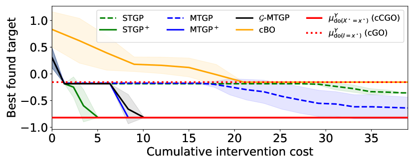
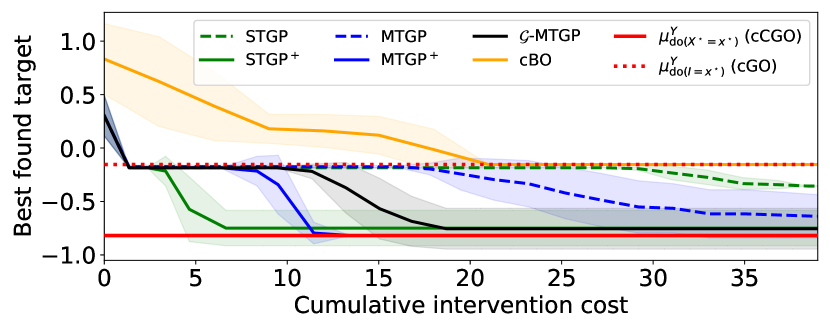
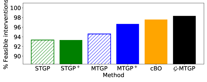
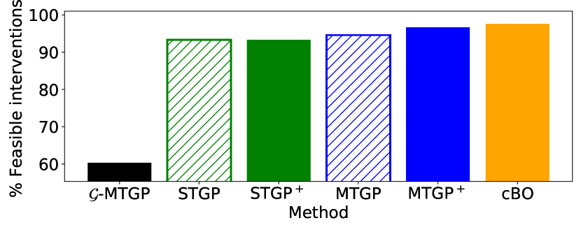
Figure 4: synthetic-2 with $N_{O}=500$ (top row) and $N_{O}=100$ (bottom row). Left: Causal graphs. Center: Convergence to the ccgo (solid red line) and cgo (dotted red line) optima. Lines give average results across different initialization of $\mathcal{D}^{I}$. Shaded areas represents $\pm$ standard deviation. Right: Average percentage of feasible interventions collected over trials.

For each model, we show the average convergence to the optimal target effect ($\pm$ standard deviations given by shaded areas), and the mean percentage of feasible interventions collected over trials across 20 initialization of $\mathcal{D}^{I}$ and for varying values of $N_{O}$. The combination of these two metrics allows us to understand how each method balances convergence speed and feasibility. To gain more insights into this balance, we also include in the analysis cbo, an algorithm that randomly picks interventions (random) and, for synthetic-1 and synthetic-2, mcbo (see Appendix C). Notice that, as cbo and mcbo solve the cgo problem, a comparison with them is only relevant for cases in which the cgo and ccgo optima are equal.

4.1 Synthetic Causal Graphs

synthetic-1. For the synthetic-1 graph with $\lambda^{X}=1$, $\lambda^{Z}=2,10$, and $N_{O}=500,100,10$ observational data samples from the scm in Appendix C.1, we obtain $n\mathbb{M}_{\C\cup Y,\mathcal{G}}=\{\{X\},\{Z\}\}$.

With $N_{O}=500$ and $\lambda^{Z}=2$, using a surrogate model that exploits $\mathcal{D}^{O}$ when constructing the prior gp parameters for functions in $g_{\mathbf{X}}(\mathbf{x})$, as in stgp⁺, mtgp⁺ and $\mathcal{G}$-mtgp, leads to faster average convergence (Fig. 3, top row). The convergence speed is further improved when capturing the covariance structure among the target and constraint effects as done by mtgp⁺ and $\mathcal{G}$-mtgp. High convergence speed for stgp⁺, mtgp⁺ and $\mathcal{G}$-mtgp is associated with a higher percentage of feasible interventions collected over trials compared to the other methods. Similar results are obtained with $N_{O}=100$ and $\lambda^{Z}=2$ (Fig. 3, bottom row) and with $N_{O}=10$ and $\lambda^{Z}=2$ (Fig. 9 in Appendix C.1). In these cases, the lower cardinality of $\mathcal{D}^{O}$ leads to a less accurate estimation of the effects which affects the prior mean functions for stgp⁺, mtgp⁺ and $\mathcal{G}$-mtgp, and kernel function for $\mathcal{G}$-mtgp. In turns, this leads to a lower number of feasible interventions and convergence speed, particularly for $\mathcal{G}$-mtgp. As a consequence, mtgp⁺ outperforms all other models in this setting. By intervening on all constrained variables ($\I=\C$) with intervention domains that are in accordance with the threshold values, cbo only collects feasible interventions. However, it converges to the higher cgo optimum, as causal structure is disregarded.

Interestingly, the results obtained with $N_{O}=500$ and $\lambda^{Z}=10$ (Fig. 10 (top row) in Appendix C.1) for which the ccgo and cgo optima are equal, making cbo, mcbo and ccbo comparable, show that both cbo and mcbo converge at a slower pace compared to mtgp⁺ and $\mathcal{G}$-mtgp while collecting a lower number of feasible interventions. Indeed, cbo and mcbo disregard the values taken by the constrained variables. Finally, when $\lambda^{Z}=10$, $\mathcal{G}$-mtgp and mtgp⁺ show fast convergence performance and high percentage of feasible interventions collected over trials. This is even when $N_{O}=100$ (Fig. 11 in Appendix C.1).

synthetic-2. For the synthetic-2 graph with $\lambda^{C}=10,\forall C\in\C$, and $N_{O}=500,100,10$ observational data samples from the scm in Appendix C.2, we obtain null-feasibility $\forall C\in\C$ and thus $n\mathbb{M}_{\C\cup Y,\mathcal{G}}=\mathcal{P}_{\I}\backslash\{A,D,E\}$. As in synthetic-1, when $N_{O}=500$ using a prior gp construction that exploits $\mathcal{D}^{O}$ leads to faster convergence (Fig. 4, top row). In particular, the accurate estimation of the target and constraint effects with $\mathcal{D}^{O}$, which are used as prior mean functions, favours the prior formulation of stgp⁺ which identifies the optimal interventions after $\sim 5$ trials. However, by disregarding the correlation among the effects, stgp⁺ collects a higher percentage of infeasible interventions compared to mtgp⁺ and $\mathcal{G}$-mtgp. In this setting, accurate estimation of the functions in the scm translates to better uncertainty estimation around the effects given by the kernel function of $\mathcal{G}$-mtgp. Therefore $\mathcal{G}$-mtgp successfully trades off improvement and feasibility showing a similar convergence to mtgp⁺ but the highest percentage of feasible interventions collected.

With $N_{O}=100$ (Fig. 4, bottom row) and $N_{O}=10$ (Fig. 12 of Appendix C.2), the estimation of the target and constraint effects and the functions in the scm from $\mathcal{D}^{O}$ deteriorates leading mtgp⁺, which learns the correlations directly from $\mathcal{D}^{I}$, to outperform all other methods.

As in synthetic-1, intervening on all variables in $\I$ simultaneously blocks the propagation of causal effects in the graph thus leading cbo to achieve a sub-optimal solution compared to ccbo and a lower number of feasible interventions compared to $\mathcal{G}$-mtgp.

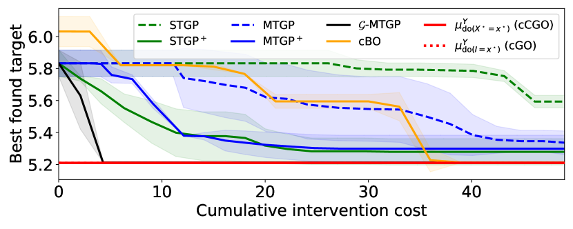
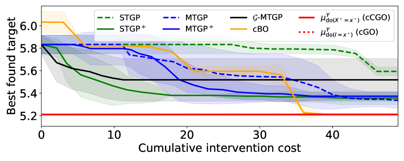
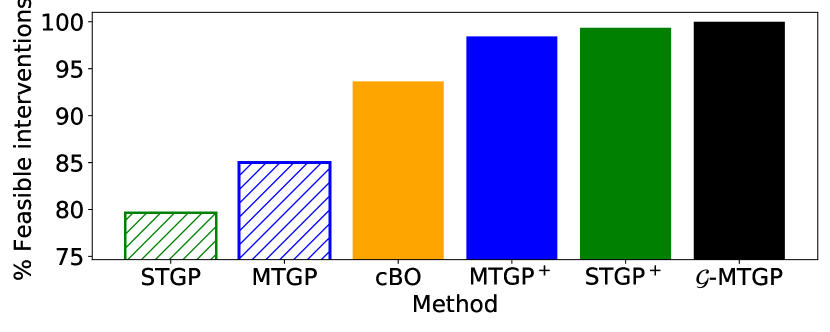
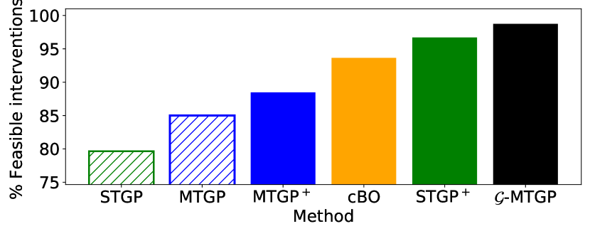
Figure 5: health with $N_{O}=100$ (top row) and $N_{O}=10$ (bottom row). Left: Causal graphs. Center: Convergence to the ccgo (solid red line) and cgo (dotted red line coinciding with the solid red line in this experiment) optima. Lines give average results across different initialization of $\mathcal{D}^{I}$. Shaded areas represents $\pm$ standard deviation. Right: Average percentage of feasible interventions collected over trials.

4.2 Real-world Causal Graphs

health. For the health graph, we use the scm in Ferro et al. (2015) (given in Appendix C.3). We consider the constraint that bmi must be lower than 25, which is considered the maximum healthy level. When both $N_{O}=100$ and $N_{O}=10$, bmi is not null-feasible thus all sets in $n\mathbb{M}_{\C\cup Y,\mathcal{G}}=\{\{\text{{ci}}\},\{\text{Aspirin},\text{{ci}}\},\{\text{Statin},\text{{ci}}\},\{\text{Aspirin},\text{Statin},\text{{ci}}\}\}$ include ci. In this setting, $\I$ is the optimal intervention set, and therefore the ccgo and cgo optima coincide.

When $N_{O}=100$, cbo is significantly slower than $\mathcal{G}$-mtgp and, by disregarding causal information, collects a lower percentage of feasible interventions over trials (Fig. 5, top row). Even though the effects are simple linear functions, the stochasticity in $\mathcal{D}^{O}$ determined by $p(\U)$ is high (Fig. 15 of Appendix C.3) compared to the previous examples and obscures their estimation. This leads to a less accurate prior mean function for $\mathcal{G}$-mtgp, stgp⁺ and mtgp⁺ which translates to a lower convergence speed for the latter two models. Despite the less accurate prior mean functions, $\mathcal{G}$-mtgp achieves the fastest convergence and the highest percentage of feasible interventions (100%) by capturing the correlation among target and constraint effects induced by the scm thus properly quantifying uncertainty around them. Collecting 100% of feasible interventions is particularly important in this setting as infeasible interventions might negatively affect patients’ health status. While $\mathcal{G}$-mtgp performs well in settings with $N_{O}=100$, it does not reach convergence when $N_{O}=10$ (Fig. 5, bottom row). Indeed, the prior mean and kernel functions estimation from $\mathcal{D}^{O}$ deteriorates when the size of the observational dataset is very small leading to an incorrect uncertainty quantification around the effects and preventing the exploration of the interventional space. This is also observed for stgp⁺ and mtgp⁺ as their prior mean function is affected by the incorrect estimation of the scm functions and thus of the target and constraint effects. This leads cbo to outperform all other methods in this setting.

protein-signaling. For the protein-signaling graph, we use the observational dataset from Sachs et al. (2005), to construct an scm (see Appendix C.4). Given $N_{O}=100,10$ observational data samples from the scm, all constrained variables are null-feasible, giving $n\mathbb{M}_{\C\cup Y,\mathcal{G}}=\{\{\textsc{pkc}\},\{\textsc{pka}\},\{\textsc{m}\text{ek}\},\{\textsc{pkc},\textsc{pka}\},\{\textsc{pkc},\textsc{m}\text{ek}\},\{\textsc{pka},\\ \textsc{m}\text{ek}\}\}$. All methods converge to the same optimum (Fig. 6). Indeed, the target effect achieved by intervening on $\I$ is equal to the one achieved by intervening on the optimal intervention set $\{\text{{pka}},\text{{m}ek}\}$ (this is the result of erk being independent on pkc and akt given mek and pka). In addition, in this example $\C_{\I}=\emptyset$ thus by intervening on $\I$ with interventional domains that are in accordance with the threshold values cbo achieves a 100% average feasibility.

Overall cbo performs comparably to $\mathcal{G}$-mtgp and mtgp⁺ (Fig. 6, top row) when $N_{O}=100$, while cbo is faster but selects more infeasible interventions (Fig. 18 in Appendix C.4). Despite achieving slower convergence than single task models, mtgp⁺ and $\mathcal{G}$-mtgp select a higher percentage of feasible interventions (99.13%) with $\mathcal{G}$-mtgp converging slightly faster then mtgp⁺. The feasibility aspect is again particularly important as every non feasible intervention results in the inhibition of pka, which can impede healthy functions of the cell. Hence, a method that yields greater than 99% feasible interventions at the cost of ($\sim 10$) additional interventions (mtgp⁺ and $\mathcal{G}$-mtgp) is deemed preferable compared to methods that explore the intervention space more aggressively but yield a lower number of feasible interventions (cbo, stgp and stgp⁺).

As in the other experiments, the convergence performance of $\mathcal{G}$-mtgp and mtgp⁺ slightly deteriorates when $N_{O}=10$ (Fig. 6, bottom row) due to an incorrect uncertainty quantification around the effects which prevents the exploration of the interventional space. As in the results for $N_{O}=100$, notice how cbo achieves a 100% average feasibility as all constrained variables are intervened ($\C\subset\I$, $\C_{\I}=\emptyset$) with interventional ranges that are in accordance with the threshold values. The algorithm quickly identify the cgo optimum, which is in this case equal to the ccgo optimum.

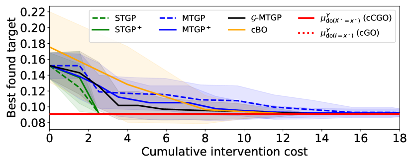
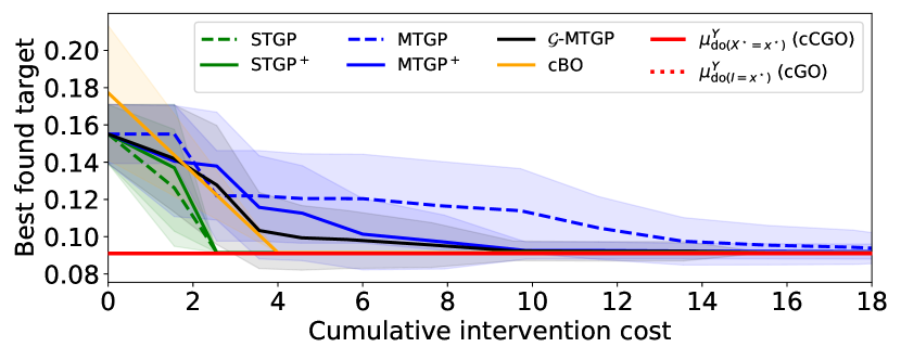
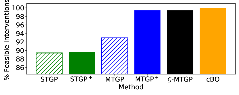
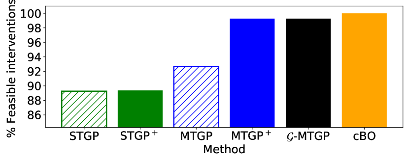
Figure 6: protein-signaling with $N_{O}=100$ and $N_{O}=10$ (bottom row). Left: Causal graphs. Center: Convergence to the ccgo (solid red line) and cgo (dotted red line coinciding with the solid red line in this experiment) optima. Lines give average results across different initialization of $\mathcal{D}^{I}$. Shaded areas represents $\pm$ standard deviation. Right: Average percentage of feasible interventions collected over trials.

5 Discussion

In this paper, we introduced the ccbo approach for identifying interventions optimizing a target effect under constraints. We proposed different gp surrogate models for the target and constraint effects that leverage observational data $\mathcal{D}^{O}$ and the structure of the scm. Our results show that incorporating $\mathcal{D}^{O}$ in the gp prior construction leads to faster identification of optimal interventions and higher percentage of feasible interventions selected. They also show that further performance improvement can be obtained using multi-task gp models which capture the correlation among target and constraint effects. Accounting for the scm structure in the covariance matrix, as done by $\mathcal{G}$-mtgp, is especially beneficial with more complex correlation structures or with a high number of effects. We found $\mathcal{G}$-mtgp to successfully trade off improvement and feasibility, achieving a fast convergence while collecting the highest percentage of feasible interventions. However, as $\mathcal{G}$-mtgp exploits the fitted scm functions in the computation of the prior parameters, when these functions cannot be learned accurately mtgp⁺ is preferable as it can learn the correlation directly from $\mathcal{D}^{I}$.

Our search space reduction procedure can be thought as placing an intervention cost for each $\mathbf{X}\in\mathcal{P}_{\I}$ that is equal to its cardinality. This procedure could be modified using different cost structures or augmented with budget constraints. For example, one could exclude from $\mathcal{P}_{\I}$ the intervention sets non satisfying a budget and then proceed by excluding sets according to the proposed procedure.

ccbo requires knowledge of the true causal graph underlying the system of interest, an assumption that might not be satisfied in practice. Using ccbo with an incorrect graph $\mathcal{G}^{\prime}$ could lead to inaccurate gp prior parameters and invalid search space reduction. Indeed, there is no guarantee that $n\mathbb{M}_{\C\cup Y,\mathcal{G}^{\prime}}$ would contain the optimal intervention set when the independence and the ancestor-type relationships encoded in $\mathcal{G^{\prime}}$ differ from those in $\mathcal{G}$. Extending the methodology to deal with settings characterized by misspecified or unknown $\mathcal{G}$, similarly e.g. to Branchini et al. (2023), represents an important future direction.

From a computational perspective, ccbo might suffer from poor scalability when $|\C|$ or the number of collected interventional data samples are high. In the latter case, sparse gp methods e.g. inducing inputs (Titsias, 2009), could be used to significantly reduce the computational complexity of both single-task and multi-task gps. Alternatively, one could consider sharing information across the surrogate models of different sets in $n\mathbb{M}_{\mathbf{C}\cup Y,\mathcal{G}}$ in order to reduce the total number of interventions. Evaluating ccbo on real-world settings where $|\C|$ is high would require simulators characterized by a high number of variables. In terms of convergence properties, while the constrained ei does not currently provide theoretical guarantees, one could extend ccbo to use a constrained acquisition function achieving asymptotic convergence, e.g. gp-ucb, (Srinivas et al., 2009; Lu & Paulson, 2022) or a non-myopic acquisition function to avoid exploration issues (Lam & Willcox, 2017).

Another future direction for safe-critical applications would be to extend the current framework to deal with safety constraints in order to guarantee that the number of feasible interventions collected never falls below a critical value. Finally, while ccbo focuses on hard interventions in which variables are set to specific values, an interesting extension would be to consider more general soft-interventions.

Appendix A Reducing the Search Space

Recall the definition of cmis relative to $(\C\cup Y,\mathcal{G})$.

Definition 3.1 (cmis).

A set $\mathbf{X}\subseteq\I$ is said to be a cmis relative to $(\C\cup Y,\mathcal{G})$ if there is no $\mathbf{X}^{\prime}\subset\mathbf{X}$ with $\C_{\mathbf{X}}=\C_{\mathbf{X}^{\prime}}$ such that $\mu_{\text{do}(\mathbf{X}=\mathbf{x})}^{W}=\mu_{\text{do}(\mathbf{X}^{\prime}=\mathbf{x}^{\prime})}^{W}$, where $\mathbf{x}^{\prime}$ indicates the subset of $\mathbf{x}$ corresponding to variables $\mathbf{X}^{\prime}$, $\forall\mathbf{x}\in D(\mathbf{X})$, $\forall W\in\C_{\mathbf{X}}\cup Y$, and $\forall$ scm with causal graph $\mathcal{G}$.

Also recall that $\mathbb{M}_{\C\cup Y,\mathcal{G}}$ is the subset of $\mathcal{P}_{\I}$ whose elements are cmiss relative to $({\C\cup Y},\mathcal{G})$, that $\text{an}(W,\mathcal{G})$ denotes the set of ancestors of $W$ in $\mathcal{G}$, that $\text{an}(\W,\mathcal{G}):=\cup_{W\in\W}\text{an}(W,\mathcal{G})$, and that $\mathcal{G}_{\overline{\mathbf{X}}}$ is the graph with all incoming edges onto all elements of $\mathbf{X}$ removed.

Proposition 3.3 (Characterization of cmis).

$\mathbf{X}\subseteq\I$ is a cmis relative to $({\C\cup Y},\mathcal{G})$ $\iff$ $\mathbf{X}\subseteq\text{an}(\C\cup Y,\mathcal{G}_{\overline{\mathbf{X}}})\cup(\C\cap\mathbf{X})$.

Proof.
($\Longrightarrow$) We first prove that if $\mathbf{X}\subseteq\text{an}(\C\cup Y,\mathcal{G}_{\overline{\mathbf{X}}})\cup(\C\cap\mathbf{X})$ then $\mathbf{X}$ is a cmis relative to $(\C\cup Y,\mathcal{G})$.

$\mathbf{X}\subseteq\text{an}(\C\cup Y,\mathcal{G}_{\overline{\mathbf{X}}})\cup(\C\cap\mathbf{X})$ implies that, for any $\mathbf{X}^{\prime}\subset\mathbf{X}$, the set $\Q=\mathbf{X}\backslash\mathbf{X}^{\prime}$ is also a subset of $\text{an}(\C\cup Y,\mathcal{G}_{\overline{\mathbf{X}}})\cup(\C\cap\mathbf{X})$. Therefore (i) $\Q\subset\text{an}(\C\cup Y,\mathcal{G}_{\overline{\mathbf{X}}})$, or (ii) $\Q\subset\C\cap\mathbf{X}$, or (iii) $\Q$ includes both variables in $\text{an}(\C\cup Y,\mathcal{G}_{\overline{\mathbf{X}}})$ and $\C\cap\mathbf{X}$. In case (ii), $\Q\subseteq\C$ and, as $\mathbf{X}=\Q\cup\mathbf{X}^{\prime}$, we obtain $\C\cap\mathbf{X}=\C\cap(\Q\cup\mathbf{X}^{\prime})=(\C\cap\Q)\cup(\C\cap\mathbf{X}^{\prime})=\Q\cup(\C\cap\mathbf{X}^{\prime})\supset\C\cap\mathbf{X}^{\prime}$ implying $\C_{\mathbf{X}}\subset\C_{\mathbf{X}^{\prime}}$ which violates the requirement $\C_{\mathbf{X}}=\C_{\mathbf{X}^{\prime}}$ of Definition 3.1. In cases (i) and (iii), $\Q$ includes at least one variable, say $Q$, with at least one directed path, say from $Q$ to $W\in\C\cup Y$, that is not passing through $\mathbf{X}^{\prime}$ (as the incoming edges into $\mathbf{X}^{\prime}$ are removed in $\mathcal{G}_{\overline{\mathbf{X}}}$). Consider a scm with $V=\sum_{i=1}^{|\text{pa}(V)|}\text{pa}(V)_{i}+U_{V}$, where $\text{pa}(V)_{i}$ is the $i$-th parent, and $U_{V}\sim\mathcal{N}(0,1)$. In this scm, $\mu_{\text{do}(\mathbf{X}^{\prime}=\mathbf{x}^{\prime})}^{W}=a\mathbf{x}^{\prime}+b\mu^{Q}_{\text{do}(\mathbf{X}^{\prime}=\mathbf{x}^{\prime})}$ where $a$ and $b$ are two positive constants, while $\mu_{\text{do}(Q=q,\mathbf{X}^{\prime}=\mathbf{x}^{\prime})}^{W}=a\mathbf{x}^{\prime}+bq$, so that taking $q=\mu_{\text{do}(\mathbf{X}^{\prime}=\mathbf{x}^{\prime})}^{Q}+1$ gives $\mu_{\text{do}(Q=q,\mathbf{X}^{\prime}=\mathbf{x}^{\prime})}^{W}>\mu_{\text{do}(\mathbf{X}^{\prime}=\mathbf{x}^{\prime})}^{W}$. Therefore, for any $\mathbf{X}^{\prime}\subset\mathbf{X}$ we can construct a scm such that $\mu_{\text{do}(\mathbf{X}=\mathbf{x})}^{W}>\mu_{\text{do}(\mathbf{X}^{\prime}=\mathbf{x}^{\prime})}^{W}$ for at least one $W\in\C\cup Y$. As there is no $\mathbf{X}^{\prime}\subset\mathbf{X}$ such that $\mu_{\text{do}(\mathbf{X}=\mathbf{x})}^{W}=\mu_{\text{do}(\mathbf{X}^{\prime}=\mathbf{x}^{\prime})}^{W}$ $\forall W\in\C\cup Y$ and $\forall$ scm with causal graph $\mathcal{G}$, $\mathbf{X}$ satisfies the requirements of Definition 3.1 for being a cmis relative to $(\C\cup Y,\mathcal{G})$.

($\Longleftarrow$) We now prove that if $\mathbf{X}$ is a cmis relative to $(\C\cup Y,\mathcal{G})$ then $\mathbf{X}\subseteq\text{an}(\C\cup Y,\mathcal{G}_{\overline{\mathbf{X}}})\cup(\C\cap\mathbf{X})$.
If $\mathbf{X}$ were not a subset of $\text{an}(\C\cup Y,\mathcal{G}_{\overline{\mathbf{X}}})\cup(\C\cap\mathbf{X})$, then we could define the non empty set $\Q=\mathbf{X}\backslash\big{(}\mathbf{X}\cap(\text{an}(\C\cup Y,\mathcal{G}_{\overline{\mathbf{X}}})\cup(\C\cap\mathbf{X}))\big{)}$ and the set $\mathbf{X}^{\prime}=\mathbf{X}\backslash\Q\subset\mathbf{X}$ such that (1) $\C_{\mathbf{X}}=\C_{\mathbf{X}^{\prime}}$ and (2) all effects on variables in $\C\cup Y$ for $\mathbf{X}^{\prime}$ and $\mathbf{X}$ are equal, contradicting $\mathbf{X}$ being a cmis relative to $(\C\cup Y,\mathcal{G})$. Condition (1) would hold as $\mathbf{X}\cap(\text{an}(\C\cup Y,\mathcal{G}_{\overline{\mathbf{X}}})\cup(\C\cap\mathbf{X}))=(\mathbf{X}\cap\text{an}(\C\cup Y,\mathcal{G}_{\overline{\mathbf{X}}}))\cup(\mathbf{X}\cap\C)$ implies that we can express $\Q$ as $\Q=\mathbf{X}\backslash(\B\cup(\mathbf{X}\cap\C))$ for $\B=\mathbf{X}\cap\text{an}(\C\cup Y,\mathcal{G}_{\overline{\mathbf{X}}})$, showing that $\Q$ does not include variables in $\mathbf{X}$ that are in $\C$, and therefore that $\C_{\mathbf{X}}=\C_{\mathbf{X}^{\prime}}$. Condition (2) would follow from the fact that the non-overlapping sets $\Q$ and $\C\cup Y$ satisfy $(\C\cup Y)\rotatebox[origin={c}]{90.0}{$\models$}_{\mathcal{G}_{\overline{\mathbf{X}}}}\Q\,|\,\mathbf{X}^{\prime}$ as: (i) there could not be causal paths from any variable in $\Q$ to any variable in $(\C\cup Y)$ in $\mathcal{G}_{\overline{\mathbf{X}}}$ (as $\Q$ does not contain the ancestors of $(\C\cup Y)$ by definition), (ii) non-causal frontdoor paths would be closed as the incoming edges into the colliders that might be included in $\mathbf{X}^{\prime}$ would be removed in $\mathcal{G}_{\overline{\mathbf{X}}}$, and (iii) all backdoor paths would be removed in $\mathcal{G}_{\overline{\mathbf{X}}}$. Therefore, by the Rule 3 of do-calculus, we would have $\mu^{W}_{\text{do}(\Q=\q,\mathbf{X}^{\prime}=\mathbf{x}^{\prime})}=\mu^{W}_{\text{do}(\mathbf{X}^{\prime}=\mathbf{x}^{\prime})}$ $\forall W\in\C\cup Y$. ∎

Theorem 3.2 (Sufficiency of $\mathbb{M}_{\C\cup Y,\mathcal{G}}$).

$\mathbb{M}_{\C\cup Y,\mathcal{G}}$ contains a solution of the ccgo problem (if a solution exists), $\forall$ scm with causal graph $\mathcal{G}$.

Proof. Consider a set $\mathbf{X}$ that satisfies Eq. (1). By Definition 3.1, if $\mathbf{X}\notin\mathbb{M}_{\C\cup Y,\mathcal{G}}$ there exists a set $\mathbf{X}^{\prime}\subset\mathbf{X}$ with $\C_{\mathbf{X}}=\C_{\mathbf{X}^{\prime}}$ such that $\mu_{\text{do}(\mathbf{X}=\mathbf{x})}^{Y}=\mu_{\text{do}(\mathbf{X}^{\prime}=\mathbf{x}^{\prime})}^{Y}$ and $\mu_{\text{do}(\mathbf{X}=\mathbf{x})}^{C}=\mu_{\text{do}(\mathbf{X}^{\prime}=\mathbf{x}^{\prime})}^{C},\;\forall C\in\C_{\mathbf{X}^{\prime}}$ and therefore $\mathbf{X}^{\prime}$ also satisfies Eq. (1). If $\mathbf{X}^{\prime}\notin\mathbb{M}_{\C\cup Y,\mathcal{G}}$, we can apply a similar reasoning, and proceed until we find a set for which there is no subset that gives the same effects, which therefore is in $\mathbb{M}_{\C\cup Y,\mathcal{G}}$. ∎

Table 1: Summary of the prior mean $m_{\mathbf{X}}^{V}(\mathbf{x})$ and kernel $S_{\mathbf{X}}^{V}(\mathbf{x},\mathbf{x}^{\prime})$ parameters associated to the different surrogate models. $\{g_{\mathbf{X}}^{V,(s)}\}_{s=1}^{S^{\prime}}$ denote a set of $S^{\prime}$ realisations of $g_{\mathbf{X}}^{V}$ obtained by sampling from $p(\U)$ and the posterior distributions of $f_{V}$ given $\mathcal{D}^{O}$, $\hat{\sigma}^{V}_{\text{do}(\mathbf{X}=\mathbf{x})}=\sqrt{\frac{1}{S^{\prime}}\sum_{s=1}^{S^{\prime}}\left(g_{\mathbf{X}}^{V,(s)}(\mathbf{x})-m_{\mathbf{X}}^{V}(\mathbf{x}\right)^{2}}$, $\sigma^{2}_{f}$ and $l$ are the kernel hyper-parameters, and $S_{\mathbf{X},q}(\mathbf{x},\mathbf{x}^{\prime})$ is the kernel function for $u_{\mathbf{X},q}$ with associated scalar coefficient $a_{\mathbf{X},q}^{V_{k}}$.

	Prior parameters for $g_{\mathbf{X}}^{V}$
	$m^{V}_{\mathbf{X}}(\mathbf{x})$	$S^{V}_{\mathbf{X}}(\mathbf{x},\mathbf{x}^{\prime})$
cbo	0	$\sigma^{2}_{f}\exp(-\frac{||\mathbf{x}-\mathbf{x}^{\prime}||^{2}}{2l^{2}})$
cbo	0	$\sigma^{2}_{f}\exp(-\frac{||\mathbf{x}-\mathbf{x}^{\prime}||^{2}}{2l^{2}})$
stgp	0	$\sigma^{2}_{f}\exp(-\frac{||\mathbf{x}-\mathbf{x}^{\prime}||^{2}}{2l^{2}})$
stgp+	$\frac{1}{S^{\prime}}\sum_{s=1}^{S^{\prime}}g^{V,(s)}_{\mathbf{X}}(\mathbf{x})$	$\sigma^{2}_{f}\exp(-\frac{||\mathbf{x}-\mathbf{x}^{\prime}||^{2}}{2l^{2}})$ + $\hat{\sigma}^{V}_{\text{do}(\mathbf{X}=\mathbf{x})}\times\hat{\sigma}^{V}_{\text{do}(\mathbf{X}=\mathbf{x}^{\prime})}$
mtgp	0	$\sum_{q=1}^{Q}\left(a^{V}_{\mathbf{X},q}\right)^{2}S_{\mathbf{X},q}(\mathbf{x},\mathbf{x}^{\prime})$
mtgp+	$\frac{1}{S^{\prime}}\sum_{s=1}^{S^{\prime}}g^{V,(s)}_{\mathbf{X}}(\mathbf{x})$	$\sum_{q=1}^{Q}\left(a^{V}_{\mathbf{X},q}\right)^{2}S_{\mathbf{X},q}(\mathbf{x},\mathbf{x}^{\prime})$
$\mathcal{G}$-mtgp	$\frac{1}{S^{\prime}}\sum_{s=1}^{S^{\prime}}g^{V,(s)}_{\mathbf{X}}(\mathbf{x})$	$\frac{1}{S^{\prime}}\sum_{s=1}^{S^{\prime}}g^{V,(s)}_{\mathbf{X}}(\mathbf{x})g^{V,(s)}_{\mathbf{X}}(\mathbf{x}^{\prime})-\Big{(}\frac{1}{S^{\prime}}\sum_{s=1}^{S^{\prime}}g^{V,(s)}_{\mathbf{X}}(\mathbf{x})\Big{)}\Big{(}\frac{1}{S^{\prime}}\sum_{s=1}^{S^{\prime}}g^{V,(s)}_{\mathbf{X}}(\mathbf{x}^{\prime})\Big{)}$

Lemma A.1.

For any disjoint set of variables $\W_{1}$, $\W_{2}$, $\W_{3}$, if $\W_{1}\cap\text{an}(\W_{2},\mathcal{G}_{\overline{\W_{1},\W_{3}}})=\emptyset$ then $\W_{2}\rotatebox[origin={c}]{90.0}{$\models$}_{\mathcal{G}_{\overline{\W_{1},\W_{3}}}}\W_{1}\,|\,\W_{3}$.

Proof. $\W_{1}\cap\text{an}(\W_{2},\mathcal{G}_{\overline{\W_{1},\W_{3}}})=\emptyset$ implies that there are no directed paths from (any element of) $\W_{1}$ to (any element of) $\W_{2}$ in $\mathcal{G}_{\overline{\W_{1},\W_{3}}}$. In addition, all backdoor paths from $\W_{1}$ to $\W_{2}$ in $\mathcal{G}$ are removed in $\mathcal{G}_{\overline{\W_{1},\W_{3}}}$. Therefore, all paths from $\W_{1}$ to $\W_{2}$ in $\mathcal{G}_{\overline{\W_{1},\W_{3}}}$ are non-directed frontdoor paths. As $\W_{3}$ cannot be a collider on paths from $\W_{1}$ to $\W_{2}$ in $\mathcal{G}_{\overline{\W_{1},\W_{3}}}$ ($\W_{3}$ does not have incoming edges in $\mathcal{G}_{\overline{\W_{1},\W_{3}}}$), these paths cannot be opened by conditioning on $\W_{3}$. In conclusion, all paths from $\W_{1}$ to $\W_{2}$ are closed in ${\mathcal{G}_{\overline{\W_{1},\W_{3}}}}$ given $\W_{3}$, therefore $\W_{2}\rotatebox[origin={c}]{90.0}{$\models$}_{\mathcal{G}_{\overline{\W_{1},\W_{3}}}}\W_{1}\,|\,\W_{3}$. ∎

Let $n\mathbb{M}_{\C\cup Y,\mathcal{G}}(\mathbf{X},C):=\{\mathbf{X}^{\prime}\in\mathbb{M}_{\C\cup Y,\mathcal{G}}:\mathbf{X}^{\prime}\supset\mathbf{X},\;\mathbf{X}^{\prime}=\mathbf{X}\cup\mathbf{X}_{1}$ with $\mathbf{X}_{1}\cap\text{an}(\C_{\mathbf{X}}\backslash C\cup Y,\mathcal{G}_{\overline{\mathbf{X}^{\prime}}})=\emptyset\;\text{and}\;\C_{\mathbf{X}^{\prime}}=\C_{\mathbf{X}}\;\text{or}\;\mathbf{X}\cap\text{an}(C^{\prime},\mathcal{G}_{\overline{\mathbf{X}}})=\emptyset\;\text{and}\;\mu^{C^{\prime}}\geq\lambda^{C^{\prime}}\;\text{for all}\;C^{\prime}\in\C_{\mathbf{X}}\backslash\C_{\mathbf{X}^{\prime}}\}$; let $n\mathbb{M}_{\C\cup Y,\mathcal{G}}(\mathbf{X}):=\Big{\{}\bigcup_{C\in\C_{\mathbf{X}},\mathbf{X}\cap\text{an}(C,\mathcal{G}_{\overline{\mathbf{X}}})=\emptyset}[\mathbf{X},n\mathbb{M}_{\C\cup Y,\mathcal{G}}(\mathbf{X},C)]_{\mu^{C}\geq\lambda^{C}}\Big{\}}$ with $[\mathbf{X},n\mathbb{M}_{\C\cup Y,\mathcal{G}}(\mathbf{X},C)]_{\mu^{C}\geq\lambda^{C}}=n\mathbb{M}_{\C\cup Y,\mathcal{G}}(\mathbf{X},C)$ if $\mu^{C}\geq\lambda^{C}$ and $\mathbf{X}$ otherwise.

Theorem A.2 (Sufficiency of $n\mathbb{M}_{\C\cup Y,\mathcal{G}}$).

$n\mathbb{M}_{\C\cup Y,\mathcal{G}}:=\mathbb{M}_{\C\cup Y,\mathcal{G}}\backslash\bigcup_{\mathbf{X}\in\mathbb{M}_{\C\cup Y,\mathcal{G}}}n\mathbb{M}_{\C\cup Y,\mathcal{G}}(\mathbf{X})$ contains a solution of the ccgo problem (if a solution exists), $\forall$ scm with causal graph $\mathcal{G}$.

Proof. Consider a set $\mathbf{X}^{\prime}\in\mathbb{M}_{\C\cup Y,\mathcal{G}}$ that satisfies Eq. (1). If $\mathbf{X}^{\prime}\not\in n\mathbb{M}_{\C\cup Y,\mathcal{G}}$, then $\mathbf{X}^{\prime}\subseteq\bigcup_{\mathbf{X}\in\mathbb{M}_{\C\cup Y,\mathcal{G}}}n\mathbb{M}_{\C\cup Y,\mathcal{G}}(\mathbf{X})$, and therefore there exist at least one set $\mathbf{X}\in\mathbb{M}_{\C\cup Y,\mathcal{G}}$ and at least one $C\in\C_{\mathbf{X}}$ with $\mathbf{X}\cap\text{an}(C,\mathcal{G}_{\overline{\mathbf{X}}})=\emptyset$ (implying $\mu_{\text{do}(\mathbf{X}=\mathbf{x})}^{C}=\mu^{C}$). If $\mu^{C}<\lambda^{C}$ then $[\mathbf{X},n\mathbb{M}_{\C\cup Y,\mathcal{G}}(\mathbf{X},C)]_{\mu^{C}\geq\lambda^{C}}=\mathbf{X}$, and thus $\mathbf{X}^{\prime}\subseteq\mathbf{X}$ implying that $\C_{\mathbf{X}^{\prime}}\supseteq\C_{\mathbf{X}}$ and therefore that $\mathbf{X}^{\prime}$ does not satisfies Eq. (1) as $\mu^{C}<\lambda^{C}$. If instead $\mu^{C}\geq\lambda^{C}$, $\mathbf{X}^{\prime}\in n\mathbb{M}_{\C\cup Y,\mathcal{G}}(\mathbf{X},C)$, and thus $\mathbf{X}^{\prime}\supset\mathbf{X}$, $\mathbf{X}^{\prime}=\mathbf{X}\cup\mathbf{X}_{1}$ with $\mathbf{X}_{1}\cap\text{an}(\C_{\mathbf{X}}\backslash C\cup Y,\mathcal{G}_{\overline{\mathbf{X}^{\prime}}})=\emptyset$. In addition, $\mathbf{X}$ has either the same constraint set of $\mathbf{X}^{\prime}$ (i.e. $\C_{\mathbf{X}^{\prime}}=\C_{\mathbf{X}}$) or is such that its additional constraints are satisfied ($\mathbf{X}\cap\text{an}(C^{\prime},\mathcal{G}_{\overline{\mathbf{X}}})$ and $\mu^{C^{\prime}}\geq\lambda^{C^{\prime}}$ for all $C^{\prime}\in\C_{\mathbf{X}}\backslash\C_{\mathbf{X}^{\prime}}$). Therefore $\mathbf{X}$ also satisfies Eq. (1). If $\mathbf{X}\not\in n\mathbb{M}_{\C\cup Y,\mathcal{G}}$ we can apply a similar reasoning and proceed until we find a set in $n\mathbb{M}_{\C\cup Y,\mathcal{G}}$. ∎
The cMISReduce procedure is given below.

cMISReduce.

First construct $\mathbb{M}_{\C\cup Y,\mathcal{G}}$ as: $\mathbb{M}_{\C\cup Y,\mathcal{G}}=\emptyset$, $\forall\mathbf{X}\in\mathcal{P}_{\I}$, if $\mathbf{X}\subseteq\text{an}(\C\cup Y,\mathcal{G}_{\overline{\mathbf{X}}})\cup(\C\cap\mathbf{X})$ add $\mathbf{X}$ to $\mathbb{M}_{\C\cup Y,\mathcal{G}}$. Then, set $n\mathbb{M}_{\C\cup Y,\mathcal{G}}$ to $\mathbb{M}_{\C\cup Y,\mathcal{G}}$. If $\mathcal{D}^{O}\neq\emptyset$, $\forall\mathbf{X}\in\mathbb{M}_{\C\cup Y,\mathcal{G}}$, $\forall C\in\C_{\mathbf{X}}$ with $\mathbf{X}\cap\text{an}(C,\mathcal{G}_{\overline{\mathbf{X}}})=\emptyset$, if $C$ is not null-feasible (according to an estimate $\hat{\mu}^{C}$ of $\mu^{C}$) remove $\mathbf{X}$ from $n\mathbb{M}_{\C\cup Y,\mathcal{G}}$. If instead $C$ is null-feasible, remove from $n\mathbb{M}_{\C\cup Y,\mathcal{G}}$ all $\mathbf{X}^{\prime}\supset\mathbf{X}$ with $\mathbf{X}^{\prime}=\mathbf{X}\cup\mathbf{X}_{1}$ where $\mathbf{X}_{1}\cap\text{an}(\C_{\mathbf{X}}\backslash C\cup Y,\mathcal{G}_{\overline{\mathbf{X}^{\prime}}})=\emptyset$ and such that $\C_{\mathbf{X}^{\prime}}=\C_{\mathbf{X}}$ or $\mathbf{X}\cap\text{an}(C^{\prime},\mathcal{G}_{\overline{\mathbf{X}}})=\emptyset$ and $\mu^{C^{\prime}}\geq\lambda^{C^{\prime}}$ for all $C^{\prime}\in\C_{\mathbf{X}}\backslash\C_{\mathbf{X}^{\prime}}$.

Appendix B Baselines and Surrogate Models

In the experimental section we compare the performance of ccbo using different surrogate models against cbo, cbo and, for synthetic-1 and synthetic-2, also against mcbo.

For the surrogate models of cbo, cbo, and stgp we assume a zero prior mean function $m_{\mathbf{X}}^{V}(\mathbf{x})=0$ and an rbf kernel $S_{\mathbf{X}}^{V}(\mathbf{x},\mathbf{x}^{\prime})=\sigma^{2}_{f}\exp(\frac{||\mathbf{x}-\mathbf{x}^{\prime}||^{2}}{2l^{2}})$ for all $\mathbf{X}\subseteq\mathcal{P}_{\I}$ and $V\in\C_{\mathbf{X}}\cup Y$. rbf kernels are also considered for the kernel functions $S_{\mathbf{X},q}(\mathbf{x},\mathbf{x}^{\prime})$, $q=1,\ldots,Q$, associated to the latent gps of mtgp and mtgp⁺. Notice that the surrogate model parameters for cbo, cbo and stgp are equal. Indeed, these methods only differ in terms of search space and acquisition functions used. cbo solves an non-causal constrained global optimization problem therefore considers only one intervention set, i.e. $\mathbf{X}=\I$, models the associated target $\mu^{Y}_{\text{do}(\I=\mathbf{x})}$ and constraint effects $\mu^{\C_{\I}}_{\text{do}(\I=\mathbf{x})}$ independently and selects interventions via the constrained expected improvement acquisition function (Gardner et al., 2014). cbo uses the same surrogate models construction but explores the intervention sets included in $n\mathbb{M}_{\C\cup Y,\mathcal{G}}$ via a standard expected improvement acquisition function thus solving an unconstrained optimization problem. Finally, stgp considers the surrogate model constructions of cbo and cbo but explores the sets included in $n\mathbb{M}_{\C\cup Y,\mathcal{G}}$ selecting interventions via a constrained expected improvement acquisition function.

For all surrogate models exploiting $\mathcal{D}^{O}$ in the gp prior mean functions (stgp⁺, mtgp⁺ and $\mathcal{G}$-mtgp), we compute $m_{\mathbf{X}}^{V}(\mathbf{x})$ for all $\mathbf{X}\in n\mathbb{M}_{\C\cup Y,\mathcal{G}}$ and $V\in\C_{\mathbf{X}}\cup Y$ by averaging the values of $V$ obtained by sampling from the fitted scm where the functions for $\mathbf{X}$ are fixed to $\mathbf{x}$. Specifically, we model each function $f_{V}$ with a gp $f_{V}(\text{pa}(v))\sim\mathcal{GP}(0,S^{V}(\text{pa}(v),\text{pa}(v)^{\prime}))$, where $\text{pa}(v)$ denotes a value taken by $\text{pa}(V)$. We use an rbf kernel defined as $S^{V}(\text{pa}(v),\text{pa}(v)^{\prime})=\sigma^{2}_{f}\exp(-\frac{||\text{pa}(v)-\text{pa}(v)^{\prime}||^{2}}{2l^{2}})$. We assume a Gaussian likelihood for $\mathcal{D}^{O}$ and compute the posterior distribution for all $f_{V}$ in closed form via standard gp updates. We then sample from $p(\U)$ and these posteriors to obtain a set of samples $\{g_{\mathbf{X}}^{V,(s)}\}_{s=1}^{S^{\prime}}$ for all $\mathbf{X}\in n\mathbb{M}_{\C\cup Y,\mathcal{G}}$. The mean functions for the target and constraint effects are then obtained as $m_{\mathbf{X}}^{V}(\mathbf{x})=\frac{1}{S^{\prime}}\sum_{s=1}^{S^{\prime}}g_{\mathbf{X}}^{V,(s)}$ with $V=Y$ and $V=C,\forall C\in\C$ respectively. A similar procedure is used to compute the kernel function $S_{\mathbf{X}}^{V,W}(\mathbf{x},\mathbf{x}^{\prime})$ for $\mathcal{G}$-mtgp. In particular, given the samples $\{g_{\mathbf{X}}^{V,(s)}\}_{s=1}^{S^{\prime}}$ and $\{g_{\mathbf{X}}^{W,(s)}\}_{s=1}^{S^{\prime}}$ for each couple of variables $(V,W)$ in $\C\cup Y$, we compute the correlation across the associated effects as $\frac{1}{S^{\prime}}\sum_{s=1}^{S^{\prime}}g^{V,(s)}_{\mathbf{X}}(\mathbf{x})g^{W,(s)}_{\mathbf{X}}(\mathbf{x}^{\prime})-\Big{(}\frac{1}{S^{\prime}}\sum_{s=1}^{S}g^{V,(s)}_{\mathbf{X}}(\mathbf{x})\Big{)}\Big{(}\frac{1}{S^{\prime}}\sum_{s=1}^{S^{\prime}}g^{W,(s)}_{\mathbf{X}}(\mathbf{x}^{\prime})\Big{)}$. See Table 1 for a summary of the prior parameters used for each surrogate model.

Similarly to cbo, mcbo solves an unconstrained optimization problem. Instead of explicitly modelling the target effect, mcbo assumes each $V\in\V$ to be of the form $V=f_{V}(\text{pa}_{\mathcal{G}}(V),\mathbf{A}_{V})+U_{V}$, where $\mathbf{A}_{V}$ is a set of action variables whose values can be set by the investigator. It then places a vector-valued gp prior on the functions $\{f_{V}\}_{V\in\V}$ and exploits the posterior distribution of this gp together with a reparameterization trick introduced by Curi et al. (2020) to derive confidence bounds for the target effect. These bounds are then used within an upper confidence bound acquisition function. Notice that, by explicitly modelling the functions in the scm, mcbo cannot deal with settings in which there are unobserved confounders.

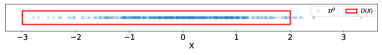
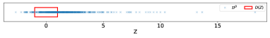
Figure 7: synthetic-1 with $N_{O}=500$. Scatter plots for the observational data together with interventional ranges $D(X)$ (top) and $D(Z)$ (bottom).

Appendix C Experimental Details and Additional Results

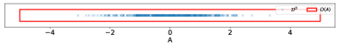
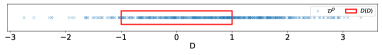
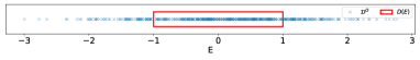
Figure 8: synthetic-2 with $N_{O}=500$. Scatter plots for the observational data together with interventional ranges $D(A)$ (top), $D(D)$ (center) and $D(E)$ (bottom).

For all experiments we initialize the kernel hyper-parameters $(\sigma^{2}_{f},l)$ of the surrogate models to 1 and optimize them with a standard type-2 ml approach. When sampling from the modified scm is required in order to compute the prior mean or kernel functions we use $S^{\prime}=10$ samples. The same number of samples is used when the computation of the acquisition function requires a Monte Carlo approximation.

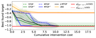
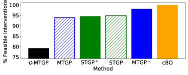
Figure 9: $\textsc{synthetic}-1$ with $N_{O}=10$ and $\lambda^{Z}=2$. Top: Convergence to ccgo (solid red line) and cgo (dotted red line) optima. Lines give average results across different initialization of $\mathcal{D}^{I}$. Shaded areas represents $\pm$ standard deviation. Bottom: Average percentage of feasible interventions collected over trials.

C.1 synthetic-1

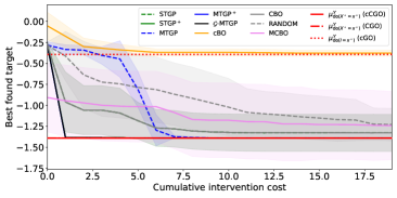
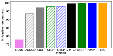
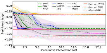
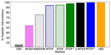
Figure 10: synthetic-1 with $N_{O}=500$ and $\lambda^{Z}=10$ (top row), and with $N_{O}=500$ and $\lambda^{Z}=2$ (bottom row). Left: Convergence to the ccgo (solid red line), cgo (dash-dotted red line) and cgo (dotted red line) optima. Right: Average percentage of feasible interventions collected over trials.

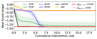
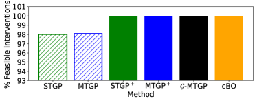
Figure 11: synthetic-1 with $N_{O}=100$ and $\lambda^{Z}=10$. Top: Convergence to the ccgo (solid red line) and cgo (dotted red line) optima. Bottom: Average percentage of feasible interventions collected over trials.

For the causal graph in Fig. 2(b) with $\I=\C=\{X,Z\}$ we consider the scm

$$X =U_{X},\,\,Z=\exp(-X)+U_{Z},$$

$$Y =\cos(Z)-\exp(-Z/20)+U_{Y},$$

with $U_{X},U_{Z},U_{Y}\sim\mathcal{N}(0,1)$. We set the interventional ranges to $D(X)=[-3,2]$ and $D(Z)=[-1,1]$, the constraint thresholds to $(\lambda^{X},\lambda^{Z})=(1,2)$ for Fig. 3, Fig. 9 and Fig. 10 (bottom row) and to $(\lambda^{X},\lambda^{Z})=(1,10)$ for Fig. 10 (top row) and Fig. 11, and require the constraint effects to be lower that the thresholds. Notice that, even in cases when $N_{O}$ is high, there exists a mismatch between the observational and interventional ranges. Fig. 7 shows how the interventional ranges are only partially covered by the observational data, especially for $X$. Therefore, estimating the target and constraint effects with $\mathcal{D}^{O}$ for interventions values outside of the observational ranges, say for $X=-2$, might lead to inaccurate results which translate to unreliable prior parameters for the surrogate models exploiting $\mathcal{D}^{O}$. A combination of interventional and observational data is needed in order to quantify uncertainty around the effects and to choose the intervention to perform next while ensuring satisfaction of the constraints, and thus to efficiently identify an optimal feasible intervention.

In this graph, $\mathcal{P}_{\I}=\{\{X\},\{Z\},\{X,Z\}\}$, and $\mathbb{M}_{\C\cup Y,\mathcal{G}}=\mathcal{P}_{\I}$ as $\mathbf{X}\subseteq\text{an}(\{X,Z,Y\},\mathcal{G}_{\overline{\mathbf{X}}})\cup(\{X,Z\}\cap\mathbf{X})$, $\forall\mathbf{X}\in\mathcal{P}_{\I}$. The set $\mathbf{X}=\{Z\}$ has only one constrained variable, $X$, that is reducible (as $\mathbf{X}\cap\text{an}(X,\mathcal{G}_{\overline{\mathbf{X}}})=\emptyset$) and null-feasible for $N_{O}=500,100,10$. We can thus exclude $\mathbf{X}^{\prime}=\{X,Z\}\supset\mathbf{X}$ from $\mathbb{M}_{\C\cup Y,\mathcal{G}}$. Indeed, $\{X,Z\}$ is of the form $\mathbf{X}^{\prime}=\mathbf{X}\cup X$ with $X\notin\text{an}(\emptyset\cap Y,\mathcal{G}_{\overline{\mathbf{X}^{\prime}}})$. We therefore obtain $n\mathbb{M}_{\C\cup Y,\mathcal{G}}=\{\{X\},\{Z\}\}$.

Fig. 10 (top row) shows the convergence results for $N_{O}=500$ and $\lambda^{Z}=10$, for which the ccgo and cgo problems have the same optimum. Notice how both cbo and mcbo converge to the optimum at a slower pace compared to stgp⁺, mtgp⁺ and $\mathcal{G}$-mtgp. Indeed, cbo and mcbo only take into account the target value observed after performing each intervention. cbo also models each function individually and, by disregarding the values of the constraints, needs to perform more interventions before identifying an optimal one. More importantly, mtgp⁺, stgp⁺ and $\mathcal{G}$-mtgp collect more than 99% of feasible interventions over trials. This is a critical aspect of the method as in real-world applications the investigator might not know whether an optimal solution is in a feasible region or not. Using ccbo in such settings does not slow down the identification of an optimal solution, but rather improves it, while allowing to efficiently restrict the exploration regions. For completeness, in Fig. 10 (bottom row) we also report the comparison with cbo, mcbo and random for $N_{O}=500$ and $\lambda^{Z}=2$.

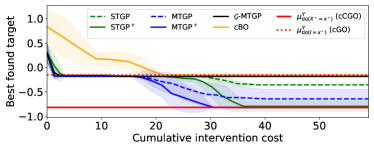
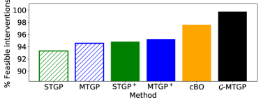
Figure 12: synthetic-2 with $N_{O}=10$. Top: Convergence to the ccgo (solid red line) and cgo (dotted red line) optima. Bottom: Average percentage of feasible interventions collected over trials.

C.2 synthetic-2

For the causal graph in Fig. 2(a) with $\I=\{A,D,E\}$ and $\C=\{C,D,E\}$ we consider the scm

$$A =U_{A},\,\,B=U_{B},$$

$$C =\exp(-A)/5+U_{C},$$

$$D =\text{cos}(B)+C/10+U_{D},$$

$$E =\exp(-C)/10+U_{E},$$

$$Y =\text{cos}(D)-D/5+\text{sin}(E)-E/4+U_{Y},$$

with $U_{A},U_{B},U_{C},U_{D},U_{E},U_{Y}\sim\mathcal{N}(0,1)$. We set the interventional ranges to $D(A)=[-5,5]$, $D(D)=[-1,1]$ and $D(E)=[-1,1]$, the constraint thresholds to $\lambda^{C}=10$, $\lambda^{D}=10$, $\lambda^{E}=10$, and require all constraint effects to be smaller than the thresholds.

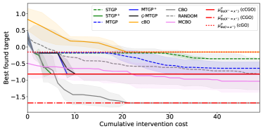
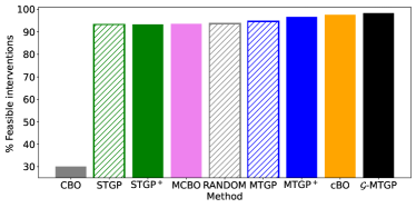
Figure 13: synthetic-2 with $N_{O}=500$. Top: Convergence to the ccgo (solid red line), cgo (dash-dotted red line) and cgo (dotted red line) optima. Bottom: Average percentage of feasible interventions collected over trials.

For $N_{O}=500,100,10$ all variables in $\C$ are null-feasible, giving $n\mathbb{M}_{\C\cup Y,\mathcal{G}}=\mathcal{P}_{\I}\backslash\{A,D,E\}=\{\{A\},\{D\},\{E\},\{A,D\},\{A,E\},\{D,E\}\}$ (see the example in Section 3.1). As in synthetic-1, even in cases when $N_{O}$ is high, there exists a mismatch between the observational and interventional ranges (Fig. 8) for all interventions sets in $n\mathbb{M}_{\C\cup Y,\mathcal{G}}$.

Fig. 12 shows the convergence plots and associated percentage of feasible interventions when $N_{O}=10$. As discussed in Section 5, when the functions in the scm cannot be learned accurately due to limited or noisy observational data, mtgp⁺ should be preferred. Indeed, a lower value for $N_{O}$ leads to a less accurate estimation of the target and constraint effects from $\mathcal{D}^{O}$ which negatively affects the prior mean functions of stgp⁺, mtgp⁺ and $\mathcal{G}$-mtgp. $\mathcal{G}$-mtgp is further penalized in this case as also the kernel functions are computed exploiting the fitted scm functions. As a consequence, we observe slower convergence and a lower percentage of feasible interventions collected when using $\mathcal{G}$-mtgp. In particular, notice how the inaccurate estimation of the constraint effects translates into a significantly lower convergence speed for $\mathcal{G}$-mtgp compared to the settings in which $N_{O}$ is higher. On the contrary, mtgp⁺ successfully trades off feasibility and improvement in these experiments reaching convergence while collecting a high percentage of feasible interventions over trials. Finally, by breaking the existing causal relationships and intervening on all variables in $\I$, cbo blocks the propagation of causal effects in the graph and converges to a solution (cgo) that is sub-optimal with respect to the one achieved by all ccbo instances.

Finally, Fig. 13 shows how, in settings where the ccgo and cgo optima differ, cbo, mcbo, and random converge to a solution which is lower than the ccgo one. In addition, by disregarding the constraints, cbo, mcbo, and random collect a high number of infeasible interventions over trials.

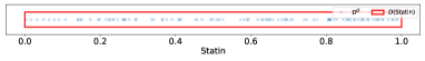
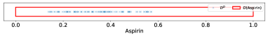
Figure 14: health with $N_{O}=100$. Scatter plots for the observational data together with interventional ranges $D(\textsc{ci})$ (top), $D(\text{Statin})$ (center) and $D(\text{Aspirin})$ (bottom).

C.3 health

For the causal graph in Fig. 1(b) with $\I=\{\text{Statin},\text{Aspirin},\textsc{ci}\}$ and $\C=\{\textsc{bmi}\}$, the scm is taken from Ferro et al. (2015) and can be written as

$$\text{Age}=U_{\text{Age}},\,\,\text{{ci}}=U_{\text{{ci}}},\,\,\text{{bmr}}=1500+10\times U_{\text{{bmr}}},$$

$$\text{Height}=175+10\times U_{\text{Height}},$$

$$\text{Weight}=\frac{\textsc{bmr}+6.8\times\text{Age}-5\times\text{Height}}{(13.7+\text{{ci}}\times 150/7716)},$$

$$\text{{bmi}}=\text{Weight}/(\text{Height}/100)^{2},$$

$$\text{Aspirin}=\sigma(-8.0+0.10\times\text{Age}+0.03\times\text{{bmi}}),$$

$$\text{Statin}=\sigma(-13.0+0.10\times\text{Age}+0.20\times\text{{bmi}}),$$

$$\textsc{psa}=6.8+0.04\times\text{Age}-0.15\times\text{{bmi}}-0.60\times\text{Statin}$$

$$\hskip 25.6073pt+0.55\times\text{Aspirin}+\sigma(2.2-0.05\times\text{Age}$$

$$\hskip 25.6073pt+0.01\times\text{{bmi}}-0.04\times\text{Statin}$$

$$\hskip 25.6073pt+0.02\times\text{Aspirin})+U_{\textsc{psa}},$$

with $U_{\text{Age}}\sim\mathcal{U}(55,75)$, $U_{\text{{ci}}}\sim\mathcal{U}(-100,100)$, $U_{\text{{bmr}}}\sim t\mathcal{N}(-1,2)$, $U_{\text{Height}}\sim t\mathcal{N}(-0.5,0.5)$, $U_{\textsc{psa}}\sim\mathcal{N}(0,0.4)$, where $\mathcal{U}(\cdot,\cdot)$ denotes a uniform random variable, $t\mathcal{N}(a,b)$ a standard Gaussian random variable truncated between $a$ and $b$, and $\sigma(\cdot)$ the sigmoidal transformation defined as $\sigma(\mathbf{x})=\frac{1}{1+\exp(-x)}$. We set the interventional ranges to $D(\text{Statin})=[0,1]$, $D(\text{Aspirin})=[0,1]$ and $D(\text{{ci}})=[-400,400]$, and require bmi to be lower than 25.

For $N_{O}=100$, these interventional ranges are only partially covered by the observational data (Fig. 14) thus significantly complicating the estimation of the effects with $\mathcal{D}^{O}$, especially when the stochasticity determined by $p(\U)$ is high (see scatter plots for ci, Statin, Aspirin and psa in Fig. 15).

We have $\mathcal{P}_{\I}=\{\{\text{Aspirin}\},\{\text{Statin}\},\{\text{{ci}}\},\{\text{Aspirin},\text{Statin}\},\\ \{\text{Aspirin},\text{{ci}}\},\{\text{Statin},\text{{ci}}\},\{\text{Aspirin},\text{Statin},\text{{ci}}\}\}$ which is equal to $\mathbb{M}_{\C\cup Y,\mathcal{G}}$. bmi is reducible for $\mathbf{X}=\{\text{Aspirin}\}$, $\mathbf{X}=\{\text{Statin}\}$ and $\mathbf{X}=\{\text{Aspirin},\text{Statin}\}$ as $\mathbf{X}\cap\text{an}(\textsc{bmi},\mathcal{G}_{\overline{\mathbf{X}}})=\emptyset$. Given an observational dataset of size $N_{O}=100,10$, $\hat{\mu}^{\textsc{bmi}}\approx 26$ making bmi not null-feasible. We therefore obtain $n\mathbb{M}_{\C\cup Y,\mathcal{G}}=\{\{\text{{ci}}\},\{\text{Aspirin},\text{{ci}}\},\{\text{Statin},\text{{ci}}\},\{\text{Aspirin},\text{Statin},\text{{ci}}\}\}$.

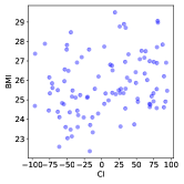
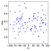
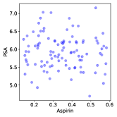
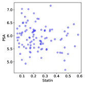
Figure 15: health. $N_{O}=100$ observational data samples from the scm in Section C.3.

For completeness we report the full comparison with cbo and random in Fig. 16. As in the previous experiments, the ccgo and cgo optima differ thus cbo and random converge, at a much lower speed, to different values while collecting a large number of infeasible interventions.

C.4 protein-signaling

For the causal graph of Fig. 1(a) with $\I=\{\text{{pkc}},\text{{pka}},\text{{m}ek},\text{{a}kt}\}$ and $\C=\{\text{{pkc}},\text{{pka}}\}$, Sachs et al. (2005) give a dataset but no scm. Thus we first fit a scm by placing a gp prior with zero mean and rbf kernel on $f_{V}$, $\forall V\in\V$, and using the observational data. We assume a Gaussian distribution with zero mean and unit variance for pkc. We use the learned scm to generate observational and interventional data.

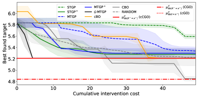
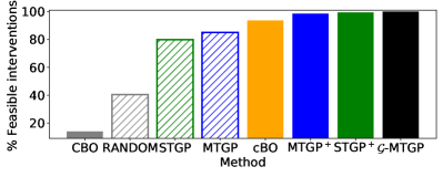
Figure 16: health with $N_{O}=100$. Top: Convergence to the ccgo (solid red line), cgo (dash-dotted red line) and cgo (dotted red line) optima. Bottom: Average percentage of feasible interventions collected over trials.

As in the previous experiments, the interventional ranges are only partially covered by $N_{O}=100$ observational samples (Fig. 17) which complicates the estimation of the effects with $\mathcal{D}^{O}$. The power set of $\I$ is given by $\mathcal{P}_{\I}=\{\{\textsc{pkc}\},\{\textsc{pka}\},\{\textsc{m}\text{ek}\},\{\text{{a}kt}\},\{\textsc{pkc},\textsc{pka}\},\{\textsc{pkc},\textsc{m}\text{ek}\},\\ \{\textsc{pkc},\text{{a}kt}\},\{\textsc{pka},\textsc{m}\text{ek}\},\{\textsc{pka},\text{{a}kt}\},\{\textsc{m}\text{ek},\text{{a}kt}\},\{\textsc{pkc},\\ \textsc{pka},\textsc{m}\text{ek}\},\{\textsc{pkc},\textsc{pka},\text{{a}kt}\},\{\textsc{pka},\textsc{m}\text{ek},\text{{a}kt}\}\}$. Note that, for $\mathbf{X}\in\{\{\text{{a}kt}\},\{\textsc{pkc},\text{{a}kt}\},\{\textsc{pka},\text{{a}kt}\},\{\textsc{m}\text{ek},\\ \text{{a}kt}\},\{\textsc{pkc},\textsc{pka},\text{{a}kt}\},\{\textsc{pka},\textsc{m}\text{ek},\text{{a}kt}\}\}$, we have $\mathbf{X}\not\subseteq\text{an}(\{\text{{pkc}},\text{{pka}},\text{{e}rk}\},\mathcal{G}_{\overline{\mathbf{X}}})\cup(\{\text{{pkc}},\text{{pka}}\}\cap\mathbf{X})$ thus we can exclude these sets from $\mathcal{P}_{\I}$ and obtain $\mathbb{M}_{\C\cup Y,\mathcal{G}}=\mathcal{P}_{\I}\backslash\{\{\text{{a}kt}\},\{\textsc{pkc},\text{{a}kt}\},\{\textsc{pka},\text{{a}kt}\},\{\textsc{m}\text{ek},\text{{a}kt}\},\{\textsc{pkc},\\ \textsc{pka},\text{{a}kt}\},\{\textsc{pka},\textsc{m}\text{ek},\text{{a}kt}\}\}$. Given $\mathcal{D}^{O}$ with size $N_{O}=100,10$, all constrained variables are null-feasible.

The set $\mathbf{X}=\{\textsc{pkc},\textsc{pka}\}$ in $\mathbb{M}_{\C\cup Y,\mathcal{G}}$ has only one constrained variable pkc that is reducible (as $\mathbf{X}\cap\text{an}(\text{{pkc}},\mathcal{G}_{\overline{\mathbf{X}}})=\emptyset$) and null-feasible for $N_{O}=100,10$. We can thus exclude $\mathbf{X}^{\prime}=\{\textsc{pkc},\textsc{pka},\textsc{m}\text{ek}\}\supset\mathbf{X}$ from $\mathbb{M}_{\C\cup Y,\mathcal{G}}$ as it is of the form $\mathbf{X}^{\prime}=\mathbf{X}\cup\textsc{pkc}$ with $\textsc{pkc}\not\in\text{an}(\emptyset\cup Y,\mathcal{G}_{\overline{\mathbf{X}^{\prime}}})=\emptyset$. We therefore obtain $n\mathbb{M}_{\C\cup Y,\mathcal{G}}=\mathbb{M}_{\C\cup Y,\mathcal{G}}\backslash\{\textsc{pkc},\textsc{pka},\textsc{m}\text{ek}\}\}$.

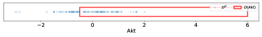
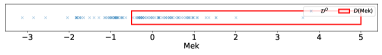
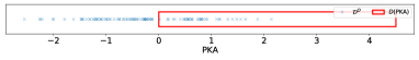
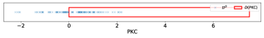
Figure 17: protein-signaling with $N_{O}=100$. Scatter plots for the observational data together with interventional ranges $D(\textsc{{a}kt})$ (top row), $D(\text{{m}ek})$ (second row), $D(\text{{pka}})$ (third row) and $D(\text{{pkc}})$ (bottom row).

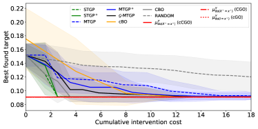
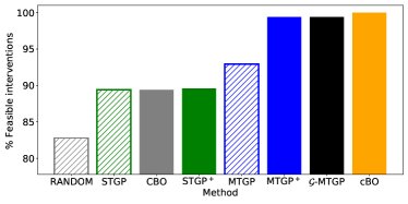
Figure 18: protein-signaling with $N_{O}=100$. Top: Convergence to the ccgo (solid red line), cgo (dash-dotted red line) and cgo (dotted red line) optima. Bottom: Percentage of feasible interventions collected over trials.

In addition, as the cgo optimum equals the ccgo optimum, cbo and random converge to the same value achieved by ccbo (Fig. 18, top row) but collect a significantly higher number of infeasible interventions (Fig. 18, bottom row).

References

- Aglietti et al. (2020) Aglietti, V., Lu, X., Paleyes, A., and González, J. Causal Bayesian optimization. In International Conference on Artificial Intelligence and Statistics, pp. 3155–3164, 2020.
- Alvarez et al. (2011) Alvarez, M. A., Rosasco, L., and Lawrence, N. D. Kernels for vector-valued functions: A review. arXiv preprint arXiv:1106.6251, 2011.
- Ariafar et al. (2019) Ariafar, S., Coll-Font, J., and Brooks, Dana Hand Dy, J. G. ADMMBO: Bayesian optimization with unknown constraints using ADMM. Journal of Machine Learning Research, 20(123):1–26, 2019.
- Atan et al. (2018) Atan, O., Jordon, J., and Van der Schaar, M. Deep-treat: Learning optimal personalized treatments from observational data using neural networks. In AAAI Conference on Artificial Intelligence, pp. 2071–2078, 2018.
- Bergmann & Graichen (2020) Bergmann, D. and Graichen, K. Safe Bayesian optimization under unknown constraints. In IEEE Conference on Decision and Control, pp. 3592–3597, 2020.
- Berkenkamp et al. (2016) Berkenkamp, F., Schoellig, A. P., and Krause, A. Safe controller optimization for quadrotors with Gaussian processes. In IEEE International Conference on Robotics and Automation, pp. 491–496, 2016.
- Berkenkamp et al. (2021) Berkenkamp, F., Krause, A., and Schoellig, A. P. Bayesian optimization with safety constraints: Safe and automatic parameter tuning in robotics. Machine Learning, pp. 1–35, 2021.
- Branchini et al. (2023) Branchini, N., Aglietti, V., Dhir, N., and Damoulas, T. Causal entropy optimization. In International Conference on Artificial Intelligence and Statistics, pp. 8586–8605, 2023.
- Bull (2011) Bull, A. D. Convergence rates of efficient global optimization algorithms. Journal of Machine Learning Research, 12(10), 2011.
- Curi et al. (2020) Curi, S., Berkenkamp, F., and Krause, A. Efficient model-based reinforcement learning through optimistic policy search and planning. Advances in Neural Information Processing Systems, 33:14156–14170, 2020.
- Dai et al. (2020) Dai, S., Song, J., and Yue, Y. Multi-task Bayesian optimization via Gaussian process upper confidence bound. In ICML 2020 Workshop on Real World Experiment Design and Active Learning, 2020.
- Eriksson & Poloczek (2021) Eriksson, D. and Poloczek, M. Scalable constrained Bayesian optimization. In International Conference on Artificial Intelligence and Statistics, pp. 730–738, 2021.
- Feliot et al. (2017) Feliot, P., Bect, J., and Vazquez, E. A Bayesian approach to constrained single-and multi-objective optimization. Journal of Global Optimization, 67(1-2):97–133, 2017.
- Ferro et al. (2015) Ferro, A., Pina, F., Severo, M., Dias, P., Botelho, F., and Lunet, N. Use of statins and serum levels of prostate specific antigen. Acta Urológica Portuguesa, 32(2):71–77, 2015.
- Frémin & Meloche (2010) Frémin, C. and Meloche, S. From basic research to clinical development of MEK1/2 inhibitors for cancer therapy. Journal of Hematology & Oncology, 3(1):1–11, 2010.
- Gardner et al. (2014) Gardner, J. R., Kusner, M. J., Xu, Z. E., Weinberger, K. Q., and Cunningham, J. P. Bayesian optimization with inequality constraints. In International Conference on Machine Learning, pp. 937–945, 2014.
- Gelbart et al. (2014) Gelbart, M. A., Snoek, J., and Adams, R. P. Bayesian optimization with unknown constraints. arXiv preprint arXiv:1403.5607, 2014.
- Griffiths & Hernández-Lobato (2017) Griffiths, R.-R. and Hernández-Lobato, J. M. Constrained Bayesian optimization for automatic chemical design. arXiv preprint arXiv:1709.05501, 2017.
- Håkansson et al. (2020) Håkansson, S., Lindblom, V., Gottesman, O., and Johansson, F. D. Learning to search efficiently for causally near-optimal treatments. In Advances in Neural Information Processing Systems, volume 33, pp. 1333–1344, 2020.
- Hakhamaneshi et al. (2021) Hakhamaneshi, K., Abbeel, P., Stojanovic, V., and Grover, A. JUMBO: Scalable multi-task Bayesian optimization using offline data. arXiv preprint arXiv:2106.00942, 2021.
- Hernández-Lobato et al. (2014) Hernández-Lobato, J. M., Hoffman, M. W., and Ghahramani, Z. Predictive entropy search for efficient global optimization of black-box functions. arXiv preprint arXiv:1406.2541, 2014.
- Keane et al. (2008) Keane, A., Forrester, A., and Sobester, A. Engineering design via surrogate modelling: a practical guide. American Institute of Aeronautics and Astronautics, Inc., 2008.
- Kirschner et al. (2019) Kirschner, J., Mutny, M., Hiller, N., Ischebeck, R., and Krause, A. Adaptive and safe Bayesian optimization in high dimensions via one-dimensional subspaces. In International Conference on Machine Learning, pp. 3429–3438, 2019.
- Lam & Willcox (2017) Lam, R. and Willcox, K. Lookahead bayesian optimization with inequality constraints. In Advances in Neural Information Processing Systems, 2017.
- Lattimore et al. (2016) Lattimore, F., Lattimore, T., and Reid, M. D. Causal bandits: Learning good interventions via causal inference. In Advances in Neural Information Processing Systems, 2016.
- Lee & Bareinboim (2018) Lee, S. and Bareinboim, E. Structural causal bandits: where to intervene? In Advances in Neural Information Processing Systems, pp. 2568–2578, 2018.
- Letham et al. (2019) Letham, B., Karrer, B., Ottoni, G., and Bakshy, E. Constrained Bayesian optimization with noisy experiments. Bayesian Analysis, 14(2):495–519, 2019.
- Lu & Paulson (2022) Lu, C. and Paulson, J. A. No-regret bayesian optimization with unknown equality and inequality constraints using exact penalty functions. IFAC-PapersOnLine, 55(7):895–902, 2022.
- Mathern et al. (2021) Mathern, A., Steinholtz, O. S., Sjöberg, A., Önnheim, M., Ek, K., Rempling, R., Gustavsson, E., and Jirstrand, M. Multi-objective constrained Bayesian optimization for structural design. Structural and Multidisciplinary Optimization, 63(2):689–701, 2021.
- Pearl (2000) Pearl, J. Causality: Models, Reasoning and Inference, volume 29. Springer, 2000.
- Pearl et al. (2016) Pearl, J., Glymour, M., and Jewell, N. P. Causal Inference in Statistics: A Primer. John Wiley & Sons, 2016.
- Picheny et al. (2016) Picheny, V., Gramacy, R. B., Wild, S., and Digabel, S. L. Bayesian optimization under mixed constraints with a slack-variable augmented Lagrangian. In Advances in Neural Information Processing Systems, pp. 1443–1451, 2016.
- Rasmussen & Williams (2006) Rasmussen, C. E. and Williams, C. K. I. Gaussian Processes for Machine Learning. The MIT Press, 2006.
- Sachs et al. (2005) Sachs, K., Perez, O., Pe’er, D., Lauffenburger, D. A., and Nolan, G. P. Causal protein-signaling networks derived from multiparameter single-cell data. Science, 308(5721):523–529, 2005.
- Schonlau et al. (1998) Schonlau, M., Welch, W. J., and Jones, D. R. Global versus local search in constrained optimization of computer models. Lecture Notes-Monograph Series, pp. 11–25, 1998.
- Snoek et al. (2012) Snoek, J., Larochelle, H., and Adams, R. P. Practical Bayesian optimization of machine learning algorithms. In Advances in Neural Information Processing Systems, volume 25, 2012.
- Sóbester et al. (2014) Sóbester, A., Forrester, A. I., Toal, D. J., Tresidder, E., and Tucker, S. Engineering design applications of surrogate-assisted optimization techniques. Optimization and Engineering, 15(1):243–265, 2014.
- Srinivas et al. (2009) Srinivas, N., Krause, A., Kakade, S. M., and Seeger, M. Gaussian process optimization in the bandit setting: No regret and experimental design. arXiv preprint arXiv:0912.3995, 2009.
- Sui et al. (2015) Sui, Y., Gotovos, A., Burdick, J., and Krause, A. Safe exploration for optimization with Gaussian processes. In International Conference on Machine Learning, pp. 997–1005, 2015.
- Sui et al. (2018) Sui, Y., Zhuang, V., Burdick, J., and Yue, Y. Stagewise safe Bayesian optimization with Gaussian processes. In International Conference on Machine Learning, pp. 4781–4789, 2018.
- Sussex et al. (2023) Sussex, S., Makarova, A., and Krause, A. Model-based causal Bayesian optimization. In International Conference on Learning Representations, 2023.
- Swersky et al. (2013) Swersky, K., Snoek, J., and Adams, R. P. Multi-task Bayesian optimization. In Advances in Neural Information Processing Systems, 2013.
- Tigas et al. (2022) Tigas, P., Annadani, Y., Jesson, A., Schölkopf, B., Gal, Y., and Bauer, S. Interventions, where and how? Experimental design for causal models at scale. In Advances in Neural Information Processing Systems, 2022.
- Titsias (2009) Titsias, M. Variational learning of inducing variables in sparse gaussian processes. In Artificial Intelligence and Statistics, pp. 567–574, 2009.
- Tran et al. (2019) Tran, A., Sun, J., Furlan, J. M., Pagalthivarthi, K. V., Visintainer, R. J., and Wang, Y. pBO-2GP-3B: A batch parallel known/unknown constrained Bayesian optimization with feasibility classification and its applications in computational fluid dynamics. Computer Methods in Applied Mechanics and Engineering, 347:827–852, 2019.
- Vazquez & Bect (2010) Vazquez, E. and Bect, J. Convergence properties of the expected improvement algorithm with fixed mean and covariance functions. Journal of Statistical Planning and Inference, 140(11):3088–3095, 2010.
- Zhang et al. (2012) Zhang, B., Tsiatis, A. A., Laber, E. B., and Davidian, M. A robust method for estimating optimal treatment regimes. Biometrics, 68(4):1010–1018, 2012.
- Zhang (2020) Zhang, J. Designing optimal dynamic treatment regimes: A causal reinforcement learning approach. In International Conference on Machine Learning, pp. 11012–11022, 2020.